IEEE TRANSACTIONS ON CONTROL SYSTEMS … Systems Dynamics... · the framework is a nonlinear model...

This article has been accepted for inclusion in a future issue of this journal. Content is final as presented, with the exception of pagination.

IEEE TRANSACTIONS ON CONTROL SYSTEMS TECHNOLOGY 1

Predictive Guidance and Control Framework for(Semi-)Autonomous Vehicles in Public Traffic

Thomas Weiskircher, Qian Wang, and Beshah Ayalew, Member, IEEE

Abstract— In this paper, a predictive trajectory guidance andcontrol framework is proposed that enables the safe operation ofautonomous and semiautonomous vehicles considering the con-straints of operating in dynamic public traffic. The core module ofthe framework is a nonlinear model predictive guidance modulethat uses a computationally expedient curvilinear frame for thedescription of the road and of the motion of the vehicle andother objects. The module enforces constraints generated frominformation about obstacles/other vehicles/objects, public trafficrules for speed limits and lane boundaries, and the limits ofthe vehicle’s dynamics. The module can be configured in twobasic modes. The first is a tracking mode, where the controlinputs computed by the model predictive guidance module act asreferences for traditional lower level control systems. The secondis a planning mode, where the traffic-optimal state trajectoriescomputed by the model predictive control are reinterpreted forplanning the optimal path and speed, which in turn can betracked by an elaborate speed and path tracking controller.The performance of most aspects of the proposed scheme isillustrated by considering various simulations of the controlframework applied to a high-fidelity vehicle dynamics model ofthe (semi-)autonomous vehicle in typical public driving events,such as intersections, passing, emergency braking, and collisionavoidance. The feasibility of the proposed control frameworkfor real-time application is highlighted with the discussions ofthe computational execution times observed for these variousscenarios.

Index Terms— Autonomous vehicles, model predictivecontrol (MPC), public traffic constraints, semiautonomousvehicles.

I. INTRODUCTION

AUTONOMOUS and semiautonomous vehicles have ahuge potential for boosting the efficiency of road trans-

portation systems via safe increases in traffic density, min-imizing pollutions, and energy waste. As such, they arecurrently under active research and development. A primaryresearch area for these vehicles is the design of robust and

Manuscript received March 31, 2016; revised August 19, 2016; acceptedDecember 2, 2016. Manuscript received in final form December 18, 2016.The work of T. Weiskircher was supported by a Post-Doctoral Fellowshipfrom the German Academic Exchange Service (DAAD). Recommended byAssociate Editor C. Canudas-de-Wit.

T. Weiskircher is with Daimler Research and Development AG,70546 Stuttgart, Germany and also with the Applied Dynamics and ControlResearch Group, International Center for Automotive Research, ClemsonUniversity, Greenville, SC 29607 USA (e-mail: [email protected]).

Q. Wang and B. Ayalew are with the Applied Dynamics and ControlResearch Group, International Center for Automotive Research, ClemsonUniversity, Greenville, SC 29607 USA (e-mail: [email protected];[email protected]).

Color versions of one or more of the figures in this paper are availableonline at http://ieeexplore.ieee.org.

Digital Object Identifier 10.1109/TCST.2016.2642164

computationally feasible control frameworks that guarantee acollision-free trajectory guidance of the vehicles under theconstraints of prevailing road boundaries, other objects, andtraffic regulations.

The majority of the existing studies in trajectory planningand guidance are found in the robotics field, where vari-ous algorithms are proposed to find collision-free trajectoriesunder static and dynamic constraints in the available space.In this discussion, the word trajectory is used to mean statetrajectories (including, at a minimum, both position or pathand speed) for the controlled robot/vehicle. The state ofthe art in planning methods roughly falls into three groups.The first are the sampling-based methods where the stateand/or input space is discretized or randomly sampled inlattices and then efficient heuristics for deterministic or sto-chastic searching, such as the A* graph search or RapidlyExploring Random Tree* algorithm is applied to find thecollision-free trajectory based on an objective function [1]–[3].However, the existence and optimality of the solutiondepends on the size of the lattice; improves with latticesize but comes at the cost of higher computational burden.A second group implements decoupling schemes for planningthe global path and for the calculation of the speed forlocal obstacle avoidance [4]. This is also a useful separationfor passenger vehicles on public roads, since the planningof the global path (often used to mean navigation or routefinding via a GPS-based navigation system employing streetmaps) and replanning in case that a collision is eminentlocally. For the problem of replanning state trajectories neardynamic obstacles, special algorithms have been proposedfor specific maneuvers, such as lane change and obstacleavoidance [5], [6]. The disadvantage of such maneuver spe-cific planning algorithms is the added need for a maneuverdetection and coordination scheme. A third group of plan-ning algorithms involve mathematical constrained optimiza-tion formulations which offer some guarantees of conditionalexistence and optimality of the solution based on the con-vexity of the problem formulation and the quality of initialguesses [7], [8].

Model predictive control (MPC), which belongs to the thirdgroup, offers a convenient and optimal replanning methodthat can accommodate dynamic changes in the environmentof the controlled vehicle via frequent updates in its recedinghorizon implementation. Although MPC could also involvelarge computational burdens as it typically solves a linear ornonlinear optimization problem at each control update, recentdevelopments in the field of real-time optimization algorithms

1063-6536 © 2017 IEEE. Personal use is permitted, but republication/redistribution requires IEEE permission.See http://www.ieee.org/publications_standards/publications/rights/index.html for more information.


2 IEEE TRANSACTIONS ON CONTROL SYSTEMS TECHNOLOGY

have made it a feasible alternative [9], [10]. In this paper, weexploit these developments to propose a control framework forpredictively guiding a road vehicle in the presence of multipledynamic public traffic constraints.

In the last decade, there has been an extensive volume ofwork in the application of MPC to vehicle dynamics control.Some works focus on collision avoidance (CA) for (semi-)autonomous systems via single control inputs, such as activefront steering [11], [12]. MPC has also been applied for lowerlevel trajectory tracking [13], [14]. Some works combine asimplified trajectory planning module with a trajectory track-ing module that uses high-fidelity nonlinear vehicle dynamicsmodels in the MPC. These models require a large set of vehicleparameters (e.g., tire data, vehicle mass, and inertia properties,which are subject to change in operation). They also requirehigh update rates consistent with the dynamics. To reducethe computational requirements, linearized models are oftenused within the MPC [15], [16]. While the execution timemay be reduced with such linearization, these assumptions donot necessarily hold during dynamic events and for vehiclesrequiring combined lateral and longitudinal control over longprediction horizons; the results are at the best suboptimal.

The key consideration for designing a real-time imple-mentable control framework for (semi-)autonomous vehiclesis in the different time scales involved in the vehicle sys-tem dynamics. While high-bandwidth actuators (e.g., steering,motors and brakes) require a control sampling of 0.001–0.01 s,vehicle dynamics control is typically executed with a sam-pling time of 0.01–0.02 s. Trajectory planning and control(or trajectory guidance, for short) is a high-level function thatneeds to interface with these lower level vehicle dynamics con-trollers. The authors estimate that feasible sampling times forMPC-based trajectory guidance are in the range of 0.05–0.15 s,with longer times needed for (semi-)autonomous driving inpublic traffic featuring dynamic obstacles and complex trafficconstraints. The computational burden of the nonlinear pro-gramming problem involved increases with the model orderor number of states, the number of control inputs, the natureof the constraints, and the length of the predictive horizon[17]. Therefore, it is important to identify formulations whichcan minimize computational overhead [18], [19].

This paper proposes a unified trajectory planning and con-trol framework for both semiautonomous and autonomousvehicles by outlining a computationally efficient model involv-ing a particle motion description of the target vehicle, theroad, and other objects in curvilinear path coordinates. Themain module in this framework is referred to as the “predictivetrajectory guidance” (PTG) module. This paper details all thecomponents of the nonlinear MPC of the PTG module, includ-ing the definitions of constraints involving vehicles/objects,road references, lane limits, traffic rules, such as speed limits,vehicle dynamics limits, and of the suitable set ups of theobjective function. Furthermore, two basic interfaces of thePTG are described along with their corresponding lower levelvehicle dynamics controllers (VDCs).

A brief version of the approach described in this paperappeared in our conference paper [20]. This paper gives signif-icantly expanded discussions. It details the derivations of the

Fig. 1. Multilevel control structure for (semi-)autonomous driving on publicroads.

motion and road model (Section III) and the cascade controlinterfacing to the vehicle dynamics control. It also gives morecomplete derivations and explanations of the MPC formula-tion, constraints and objective definitions (Section IV), andconfigurations for autonomous and semiautonomous driving.We detail the discussion of the parameterization for objectdistance constraints (Section IV-B2). After introducing theMPC formulation, we remark on the computational burdenof solving the optimization problem posed in the MPC.Furthermore, to show the broad applicability of the proposedframework, the results section includes new and updatedscenarios compared with [20]. We do defer some details onthe lower level vehicle dynamics control options to our priorwork [21]. Also, reconfigurations to enable a specific predic-tive advanced driver assistance mode (called pADAS mode)appeared in [22].

The remainder of this paper is structured as follows.Section II gives the general control framework. Section IIIdescribes the particle model used in the PTG level and itsrelation to the bicycle model commonly used for vehicledynamics modeling/control. Section IV details the MPC for-mulation. Section V briefly reviews two options for interfacingthe PTG and the vehicle dynamics controllers. Section VIpresents results and discussions. Section VII summarizes theconclusions.

II. CONTROL FRAMEWORK

Fig. 1 shows the multilevel modular framework that canbe used to facilitate the discussion of the different interactingfunctions involved in the control of (semi-)autonomous vehi-cles. At the top is an assigner module that integrates/fuses thedata from the environment perception (cameras, lidar, radar,and so on), route precalculations from navigation/GPS module,vehicle dynamics sensing/estimation modules, and prevailingtraffic rules and limits, to select the proper references andconstraints for the PTG module. The assigner module can


WEISKIRCHER et al.: PREDICTIVE GUIDANCE AND CONTROL FRAMEWORK FOR (SEMI-)AUTONOMOUS VEHICLES 3

Fig. 2. Definitions of the curvilinear motion description.

be modeled with several finite state machines that set upthe optimization problem for the PTG in different maneu-vers, such as cruising, following, leading, or changing lanes.Detailed discussions of the assigner module can be foundin [23] and [24].

At the PTG level, an MPC algorithm computes the feasibleand optimal control inputs for the target vehicle subject to theprevailing constraints and specified objective function. In [21],we identified two options for interfacing the PTG to the VDClevel. The first is called a “tracking mode” for the PTG,where its computed optimal input signals (desired longitudinalacceleration and yaw rate of the model used in the MPC) are tobe tracked by a feedback plus feed-forward lower level VDC.In the second option, called “planning mode,” the PTG merelycomputes/plans the optimal state trajectories which are thenreinterpreted by a trajectory preparation module for a pathand speed tracking VDC.

Both autonomous or semiautonomous driving can berealized with the above-mentioned framework [20]. In theautonomous mode, the PTG is considered to track both thereference velocity and lateral position via the accelerator/brakeinputs (longitudinal actuation) and active steering (lateralactuation). While in semiautonomous mode, a human driveris responsible for either the longitudinal or the lateral control,while the PTG takes charge of the other.

III. VEHICLE MODELS AND CASCADE

MODEL PARTITIONING

This section details the particle model used in the PTG leveland its relation to the bicycle model commonly used forvehicle dynamics modeling/control.

A. Particle Motion Model

To detail the model used in the PTG level, we considerthe vehicle’s motion in relation to a reference path, i.e., aroad or lane centerline as shown in Fig. 2. The curvilinearmotion of a particle, coincident with the vehicle’s center ofgravity (CG), is formulated in the Frenet n/t frame withthe n- and t- axes normal and tangential, respectively, to itsactual path. Introducing a similar frame ns/ts for the referencepath, the alignment error between the reference frame and

the vehicle/particle fixed frame denoted by ψe (see Fig. 2), isgiven by

ψe = ψp − ψs (1)

where ψp gives the vehicle’s heading, which is represented bythe orientation of the n/t frame attached to the particle/CGwith respect to the global frame Xg/Yg . ψs is the rotation ofthe road frame (labeled with s) with respect to the same globalframe. The lateral displacement ye parallel to the ns directionlocates the particle/CG laterally in relation to the referencepath. Its evolution is given by

ye = vt sin(ψe) (2)

where vt is the forward velocity of the particle/vehicle’s CG,which is always tangent to the t-axis of the particle motionframe.

Next, consider the particle motion projected on the referencepath frame. Using the projection of the particle speed on thereference path frame as shown in Fig. 2, the tangential speedvs

t and the dynamics of the arc length s read

vst = vt cos(ψe) = (ρ(s)− ye)ψs (3a)

s = ds

dt= ρ(s)ψs (3b)

with ρ(s) the distance to the center of instantaneous rotation,which can be written as a function of s. Combining theseequations, the arc length dynamics, which can also be viewedas the vehicle speed projected on the reference path, aregiven by

s = vt cos(ψe)

(ρ(s)

ρ(s)− ye

). (4)

Then, the rotation of the road frame follows:ψs = s

ρ(s)= vt cos(ψe)

(1

ρ(s)− ye

). (5)

We assume that the road curvature κ(s) = ρ(s)−1 is knownalong the arc length s. We also find that using road curvatureinstead of the road radius has at least two advantages inour modeling. First, straight roads are dealt with readily bysetting the curvature κ(s) = 0, while the radius would go toinfinity and pose numerical difficulties. Second, many roadswould involve continuous evolution of finite curvature valuesthat change signs, while using radius would involve jumps,e.g., +∞ and goes to −∞. Furthermore, we approximateavailable road curvature information in fitted-polynomial form

κ(s) = cκ,0 + cκ,1s + cκ,2s2 + cκ,3s3 + · · · (6)

where cκ,i , i = 0, 1, 2, . . . are the polynomial coefficients.These coefficients are assumed to be mapped to the real roadcurvature by a suitable algorithm within the environmentalperception module. Typically, a high-order polynomial (≥ 10)may be needed to sufficiently describe the reference pathfor a selected predictive horizon. Other feasible ways todescribe the reference path include using combinations ofGaussian or hyperbolic functions, especially for describing thecombinations of straight roads and sharp corners as usuallyfound in urban environments.



Introducing at for the longitudinal acceleration of thevehicle’s CG (in particle description), the final model for thecurvilinear particle motion description is given by

vt = at (7a)

ψe = ψp − vt cos(ψe)

(κ(s)

1 − yeκ(s)

)(7b)

ye = vt sin(ψe) (7c)

s = vt cos(ψe)

(1

1 − yeκ(s)

). (7d)

In addition, assuming that the (lower level) closed-loopvehicle dynamics exhibits a first-order lag behavior, thegeneration of at and ψp by the controlled vehicle canbe approximated by the first-order dynamics with timeconstants Tat and Tψp

as follows:at = 1/Tat (at,d − at ) (8a)

ψp = 1/Tψp(ψp,d − ψp). (8b)

Note that the time constants Tat and Tψpare the only para-

meters in the model described earlier that are related to thecontrolled vehicle. The masking of this first-order closed-loopcontrolled dynamics in the overall cascade control setup isshown in Fig. 5. It is also possible to introduce a higher orderdynamics model for the controlled vehicle to replace this first-order approximation at the cost of increased computationalburden.

Remark 1: From (8a) and (8b), the desired longitudinalacceleration at,d and the desired yaw rate ψp,d are consideredas the control inputs to the entire model described thus far.However, given the quadratic objective functions we shall poselater for the MPC in the predictive guidance module, it isoften desired to minimize the control input. However, thiscontradicts, for example, path tracking objectives in steadyturning, which require ψp = an/vt �= 0, where an isthe lateral/normal acceleration. It is, therefore, convenientto introduce a new control input �ψp,d , which describesthe deviation from a nominal yaw rate ψp,r necessary tofollow the reference path at the current speed. Formally, wewrite

ψp,d = ψp,r +�ψp,d (9a)

= vtκ(s)+�ψp,d . (9b)

In fact, by assuming a free road and no external distur-bances, the particle can follow the given reference path κ(s)under ψp,r with new control input �ψp,d = 0, whichis consistent with an input minimization objective inthe MPC.

Substituting (9b) into (8b), we note that the final inputs tothe motion model are at,d and �ψp,d .

B. Relationships Between Particle MotionDescription and Bicycle Model

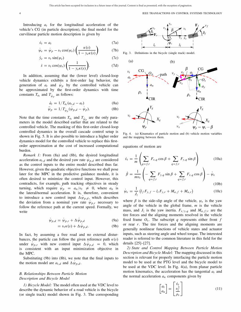
1) Bicycle Model: The model often used at the VDC level todescribe the dynamic behavior of a road vehicle is the bicycle(or single track) model shown in Fig. 3. The corresponding

Fig. 3. Definitions in the bicycle (single track) model.

Fig. 4. (a) Kinamatics of particle motion and (b) vehicle motion variablesand the mapping between them.

equations of motion are

vt = 1

m

⎛⎝ ∑

q= f,r

Fx,q cosβ +∑

q= f,r

Fy,q sin β

⎞⎠ (10a)

β = 1

mvt

⎛⎝−

∑q= f,r

Fy,q sin β +∑

q= f,r

Fx,q cosβ

⎞⎠ − ψv

(10b)

ψv = 1

Jz

(l f Fy, f − lr Fy,r + Ma, f + Ma,r

)(10c)

where β is the side-slip angle of the vehicle, ψv is the yawangle of the vehicle in the global frame, m is the vehiclemass, and Jz is the yaw inertia. Fx/y,q and Ma, f/r are thetire forces and the aligning moments resolved in the vehiclefixed frame Ov . The subscript q represents either front for rear r . The tire forces and the aligning moments aregenerally nonlinear functions of vehicle states and actuatorinputs, such as steering angle and wheel torque. The interestedreader is referred to the common literature in this field for thedetails [25]–[27].

2) State and Control Mapping Between Particle MotionDescription and Bicycle Model: The mapping discussed in thissection is relevant for properly interfacing the particle motionmodel to be used at the PTG level and the bicycle model tobe used at the VDC level. In Fig. 4(a), from planar particlemotion kinematics, the acceleration has the tangential at andthe normal acceleration an components given by

[at

an

]=

⎡⎣ vt

v2t

ρs

⎤⎦ (11)



with ρs representing the distance to the instantaneous centerof the actual vehicle path. Note that the angular deviationbetween the particle attached frame Op and the vehicleattached (body-fixed) frame Ov is the side-slip angle β, asshown in Fig. 4(b). Therefore, we have

ψp = ψv − β. (12)

From kinematics, the centrifugal acceleration is determined byits rotational speed and the distance to the center of rotation.Thus, for the particle and the vehicle’s CG (instantaneouslycoincident), we have

ψp = vt

ρs= ψv − β (13)

and thus

an = v2t

ρs= vt ψp = vt (ψv − β). (14)

This eliminates the need for knowing ρs , which is hard todetermine in (11). Instead, using vehicle states ψv and β,one can determine the accelerations for the particle motionmodel from the vehicle dynamics. This approach is used inthe closed-loop simulation results to be presented later. Also,one can easily show that the relations between the vehicle’sacceleration and velocity at the CG resolved in the vehicleattached frame Ov and that of the particle motion frame Op

are given by [ax

ay

]=

[at cosβ + an sin βat sin β − an cosβ

](15a)

[vx

vy

]=

[vt cosβvt sin β

]. (15b)

Remark 2: As different models are used in the PTG andVDC levels, a transformation of the particle motion controlinputs at,d and �ψp,d computed in the PTG is needed tomeet the specifications of the control systems in VDC. Forexample, these control systems usually use the vehicle yawrate (ψv ) as control reference to manipulate the motion ofthe vehicle and its directional stability [28], [29]. Therefore,using (9) and (13), we have

ψv,d = ψp,d + β = vtκ(s)+�ψp,d + β (16)

where measured or estimated information is assumed tobe available about the side-slip angle β and its derivative.In addition, for acceleration control, the particle motion controlinputs at,d and �ψp,d can be transformed to the vehicleattached frame via (9), (14), and (15a)[

ax,d

ay,d

]=

[at,d cosβ − vt (vtκ(s)+�ψp,d ) sin βat,d sin β + vt (vtκ(s)+�ψp,d) cosβ

]. (17)

Either these or the desired acceleration [at,d an,d ]T (withproper transformations, an,d = vt�ψp,d) can be used as con-trol references for the control systems at the VDC level. If theside-slip angle information is not available, the assumptionsβ ≈ 0 and β ≈ 0 can be made for some maneuvers.

Finally, we remark that it is also possible to establish similarrelationships between the particle motion model and otherhigher fidelity vehicle dynamics models, should one need toreplace the bicycle model at the VDC level.

Fig. 5. Cascade control setup.

C. Cascade Control Setup

Fig. 5 shows the cascade control setup that interfaces thePTG and VDC levels. Herein, in the PTG level, vehiclereferences, such as desired velocity vt,r , desired lateralposition ye,r , and curvature of the reference path κ(s), arecompared with the particle motion states which are interpretedfrom the vehicle dynamics states according to the discussionin the Section III.B. The tracking errors are used by the PTGmodule to generate the desired control inputs at,d and �ψp,d

for the particle motion model. These inputs are then sent to andinterpreted by the control systems at VDC level to generateappropriate actuation to the vehicle. In this particular setup ofFig. 5, the VDC uses the front and rear steering angles δ f

and δr , the rear wheel drive torque τd , and the brake torquesτb, f/r to control the vehicle’s dynamics. The application ofrear steering can improve the agility and stability in trackingthe reference from the PTG level. In the Sections IV and V,the PTG and VDC levels will be discussed in detail.

IV. PREDICTIVE TRAJECTORY GUIDANCE

LEVEL: MPC FORMULATION

A. Traffic, Lane, and Vehicle Dynamics Limits

We first express the lane limits and traffic restrictions,such as speed limits and stop signs, using a similar approachadopted for the definition of the curvature of the referencepath (road/lane centerline) by (6). Many of these limits aregenerally functions of the spatial position as the independentvariable, while the model outlined earlier is posed with timeas the independent variable. The introduction of the arc lengths as one of the particle motion state variables [see (7d)]simplifies the statement of the relevant constraints therebyovercoming a potential problem with mixed independent vari-ables. For example, upper speed limits v t (s) as well as theupper and lower lateral position/lane limits ye(s), y

e(s) can

be expressed as

v t (s) = c0,v + c1,vs(t)+ c2,vs(t)2 + c3,vs(t)

3 + · · · (18a)

ye(s) = c0,ll + c1,ll s(t)+ c2,ll s(t)2 + c3,ll s(t)

3 + · · · (18b)

ye(s) = c0,lr + c1,lr s(t)+ c2,lr s(t)2 + c3,lr s(t)3 + · · · (18c)

s(t) ≤ s(t) (19)

where ci,v , ci,ll , andci,lr , i = 0, 1, 2, . . . are the polynomialcoefficients may be computed by the assigner module (Fig. 1)using information of the environmental sensors and trafficrestrictions. s(t) is used to limit the longitudinal position ofthe autonomously controlled vehicle (ACV) such as necessaryto enforce a stop sign or red traffic light. It should also benoted that the definitions of ye(s) and y

e(s) are relative to



Fig. 6. Definitions of acceleration limits.

the reference path and not in the absolute/inertial frame Og .Then, straightforward inequality constraints can be added forthe speed and lateral position of the vehicle as

�v t = v t (s)− vt ≥ 0 (20a)

�ye = ye(s)− ye ≥ 0 (20b)

�ye

= ye − ye(s) ≥ 0. (20c)

Overbars and underbars indicate the upper and lower limits,respectively.

We also apply the well-known tire-road friction ellipse,which constrain the longitudinal and lateral accelerations, asshown in Fig. 6

(μH g − ζgg)2 ≥

(an,d

an,gg

)2

+ (at,d)2 (21a)

an,d = vt (κ(s)vt +�ψp,d) (21b)

0 ≤ ζgg ≤ ζ gg (21c)

0 ≤ s ≤ s. (21d)

Herein, the first constraint in (21a) is intended to restrictthe input accelerations at,d and an,d [an,d is derivedfrom (9) and (14)] to the physical ability of the tire/roadcontact patch. This is represented by the elliptical region withhalf minor/major axes μH g − ζgg and an,gg(μH g − ζgg) inFig. 6. μH is the maximum friction coefficient of the tire/roadcontact patch. The normalization coefficient an,gg ≤ 1 pro-vides a parameterization for tuning the lateral accelerationlimit. The slack variable ζgg and its upper limit ζ gg wereintroduced in [20]. These make it possible to lower the vehicleaccelerations for the sake of more comfortable trajectoriesexcept in critical maneuvers, where the slack variable allowsfull use of the acceleration potential. The slack variableζgg is formulated to track a desired value ζgg,r and thetwo norm of the tracking error ζgg − ζgg,r is weighted inthe objective function of the MPC in the PTG level. Thisformulation is often called a soft constraint. Furthermore, theconstraints

at,d ≤ at,d ≤ at,d (22a)

an,d ≤ (vtκ(s)+�ψp)vt ≤ an,d (22b)

limit the control inputs to the physical potential of the vehiclefrom actuation perspectives by adding limits for braking at,d ,traction at,d , and steering an,d , an,d . The hatched area inFig. 6 shows the final available acceleration input space (hardconstraints on an,d are omitted for clarity).

Fig. 7. Object motion definition (κ = 0) in road reference frame.

B. Spatial Constraints for Other Objects on the Road

1) Definitions of Objects for CA: One method of definingother objects to avoid is to use potential fields as used ina previous work [30]. However, that approach will allowthe vehicle to crash into an obstacle if the weightings inthe objective function are not selected properly. A properweighting is hard to find in the presence of multiple objectsand other competing terms in the cost function. Therefore,in this paper, we outline a new approach, where each objectmoves along the curvilinear frame of the reference path withits own longitudinal and lateral speeds and accelerations. Thisinformation is assumed to be obtained by the top-level assignermodule from vehicle-to-vehicle communication. During anMPC prediction horizon (between updates), we assume thatall objects follow their path with the constant longitudinal andlateral accelerations as

t,oiand as

n,oi, starting at their position

soi ,0 and ye,oi ,0, and speed vst,oi

and vsn,oi

at the beginningof the prediction. These speeds and accelerations are definedin the path curvilinear frame. With this assumption, the arclength soi and the lateral distance ye,oi to the reference line(the center of the road lane) for the ith object are given by(see Fig. 7)

soi = soi ,0 + vst,oi

xt + 1

2as

t,oix2

t (23a)

ye,oi = ye,oi ,0 + vsn,oi

xt + 1

2as

n,oix2

t (23b)

xt = 1. (23c)

The state xt is added in order to trace the MPC internaltime. At each MPC update, the initial value of xt will beset to zero. This allows for calculating the positions of theobjects in the prediction horizon using only the measurementof vs

t,oi, vs

n,oi, as

t,oi, and as

n,oi. This is done without introducing

additional motion states for each object as we did in aprevious work [30]. Herein, no heading error of the objectsis assumed. This is equivalent to the practical assumption thatthe object recognition module can project the object speeds tothe road frame. With these object positions computed over theprediction horizon, elliptical constraints can be used to restrictthe ACV from getting close to and colliding with any object

1 ≤(

ye−ye,oi�ye,oi

)2 +(

s−soi�soi

)2. (24)

Herein, �ye,oi is the lateral width plus clearance of theobject i , and thus, it is the distance of the ACV to theobject when passing; and �soi is the distance and clearanceto the vehicle along the arc length. It should be noted that the



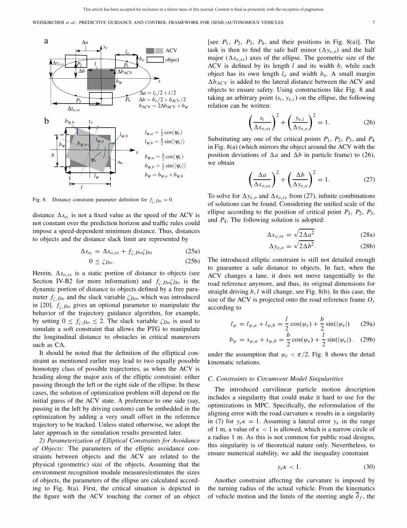
Fig. 8. Distance constraint parameter definition for fζ,Do = 0.

distance �soi is not a fixed value as the speed of the ACV isnot constant over the prediction horizon and traffic rules couldimpose a speed-dependent minimum distance. Thus, distancesto objects and the distance slack limit are represented by

�soi = �so,ss + fζ,DoζDo (25a)

0 ≤ ζDo. (25b)

Herein, �so,ss is a static portion of distance to objects (seeSection IV-B2 for more information) and fζ,DoζDo is thedynamic portion of distance to objects defined by a free para-meter fζ,Do and the slack variable ζDo, which was introducedin [20]. fζ,Do gives an optional parameter to manipulate thebehavior of the trajectory guidance algorithm, for example,by setting 0 ≤ fζ,Do ≤ 2. The slack variable ζDo is used tosimulate a soft constraint that allows the PTG to manipulatethe longitudinal distance to obstacles in critical maneuverssuch as CA.

It should be noted that the definition of the elliptical con-straint as mentioned earlier may lead to two equally possiblehomotopy class of possible trajectories, as when the ACV isheading along the major axis of the elliptic constraint: eitherpassing through the left or the right side of the ellipse. In thesecases, the solution of optimization problem will depend on theinitial guess of the ACV state. A preference to one side (say,passing in the left by driving custom) can be embedded in theoptimization by adding a very small offset in the referencetrajectory to be tracked. Unless stated otherwise, we adopt thelater approach in the simulation results presented later.

2) Parameterization of Elliptical Constraints for Avoidanceof Objects: The parameters of the elliptic avoidance con-straints between objects and the ACV are related to thephysical (geometric) size of the objects. Assuming that theenvironment recognition module measures/estimates the sizesof objects, the parameters of the ellipse are calculated accord-ing to Fig. 8(a). First, the critical situation is depicted inthe figure with the ACV touching the corner of an object

[see P1, P2, P3, P4, and their positions in Fig. 8(a)]. Thetask is then to find the safe half minor (�ye,o) and the halfmajor (�so,ss) axes of the ellipse. The geometric size of theACV is defined by its length l and its width b, while eachobject has its own length lo and width bo. A small margin�bAC V is added to the lateral distance between the ACV andobjects to ensure safety. Using constructions like Fig. 8 andtaking an arbitrary point (si , ye,i ) on the ellipse, the followingrelation can be written:(

si

�so,ss

)2

+(

ye,i

�ye,o

)2

= 1. (26)

Substituting any one of the critical points P1, P2, P3, and P4in Fig. 8(a) (which mirrors the object around the ACV with theposition deviations of �a and �b in particle frame) to (26),we obtain (

�a

�so,ss

)2

+(�b

�ye,o

)2

= 1. (27)

To solve for �ye,o and �so,ss from (27), infinite combinationsof solutions can be found. Considering the unified scale of theellipse according to the position of critical point P1, P2, P3,and P4. The following solution is adopted:

�so,ss =√

2�a2 (28a)

�ye,o =√

2�b2. (28b)

The introduced elliptic constraint is still not detailed enoughto guarantee a safe distance to objects. In fact, when theACV changes a lane, it does not move tangentially to theroad reference anymore, and thus, its original dimensions forstraight driving b, l will change, see Fig. 8(b). In this case, thesize of the ACV is projected onto the road reference frame Os

according to

lψ = lψ,a + lψ,b = l

2cos(ψe)+ b

2sin(|ψe|) (29a)

bψ = sψ,a + sψ,b = b

2cos(ψe)+ l

2sin(|ψe|). (29b)

under the assumption that ψe < π/2. Fig. 8 shows the detailkinematic relations.

C. Constraints to Circumvent Model Singularities

The introduced curvilinear particle motion descriptionincludes a singularity that could make it hard to use for theoptimizations in MPC. Specifically, the reformulation of thealigning error with the road curvature κ results in a singularityin (7) for yeκ = 1. Assuming a lateral error ye in the rangeof 1 m, a value of κ < 1 is allowed, which is a narrow circle ofa radius 1 m. As this is not common for public road designs,this singularity is of theoretical nature only. Nevertheless, toensure numerical stability, we add the inequality constraint

yeκ < 1. (30)

Another constraint affecting the curvature is imposed bythe turning radius of the actual vehicle. From the kinematicsof vehicle motion and the limits of the steering angle δ f , the



vehicle wheel base lwb, and track width btr , the curvature limitfor a front-steered vehicle is given by [26]

κ = 1btr2 + lwb

sin δ f

. (31)

This would be used to put a constraint on the yaw rate inputto be computed from (9) as

ψp,d = vtκ +�ψp,d ≤ vtκ. (32)

D. MPC Formulation

We now outline the nonlinear MPC scheme for thePTG module using the models and constraints detailed sofar. To this end, we first recall and define some MPC relatednotations. The MPC implementation we outline solves adiscretized optimization problem over a receding predictionhorizon. We denote each discretization step by k for k ∈(1, 2, . . . , Np) with the prediction horizon length Np andsampling time step �T of the model discretization, whereNp = Hp/�T . Suppose the prediction is started at theabsolute time t0, at prediction step k, the state xk denotes thepredicted motion at absolute time t = t0+k�T . As our versionof the MPC solver does not allow a separate slack in the cost,the two slack variables mentioned earlier are introduced asadditional model states with the auxiliary dynamics

ζgg = uζ,gg (33a)

ζDo = uζ,Do. (33b)

Therefore, two additional inputs need to be added for theMPC optimization to accommodate these states. Note that,while it is possible to treat the two slack variables as inputs inthe optimization, we opt to treat them as states with alloweddynamic change between discretization steps.

The finite horizon optimization problem to be solved in theMPC is the following:

minu1,...,uNp−1

Np∑k=1

||yk − rk ||2Q︸︷︷︸reference tracking

+Np−1∑k=0

||uk − ur,k ||2R︸︷︷︸control minimization

(34)

subject to

x = f (x, u) (35a)

x(t0) = x0 (35b)

xk = x(t0 + k�T ) (35c)

yk = h(xk) (35d)

rk = r(t0 + k�T ) (35e)

uk = u(t0 + k�T ) (35f)

ur,k = ur (t0 + k�T ) (35g)

c(x, u) ≤ 0 (36)

where

x = [vt ye ψe s xt at ψp ζgg ζDo]T (37a)

y = [ye vt ζgg eζ,Do]T (37b)

r = [ye,r vt,r ζgg,r eζ,Do,r]T (37c)

u = [at,d �ψp,d uζ,gg uζ,Do]T (37d)

ur = [at,d,r �ψp,d,r uζ,gg,r uζ,Do,r ]T . (37e)

The objective function by (34) penalizes the summation ofthe equidistantly sampled [see (35c)–(35g)] reference trackingand control errors. Q and R are appropriate positive semidefineweighting matrices. The augmented state equations (35a),with the augmented state vector given by (37a), are assumeddiscretized with sample time �T with piecewise constantinputs u at prediction steps k. The problem is then to minimizethe objective function subject to the equality constraints in (35)and inequality constraints compactly represented by (36).

For reference tracking, the relevant errors to minimize arethose between the system outputs in y [(37b)] and theirrespective references in r [(37c)]. The system outputs includethe speed vt and lateral position ye of the particle modeland the two slack variables. The references for the speed vt,r

and lateral position ye,r are specified by the assigner moduleaccording to the environmental and route/navigation infor-mation. The reference for the slack variable ζgg is selectednear the upper bound ζ gg , which directly defines the reduc-tion of the vehicle acceleration/handling limit [see (21a)].For the last output component eζ,Do, which is defined byeζ,Do = vt − ζDo, the reference is simply set to a zerovalue. With this selection, the distance slack variable is madeautomatically speed dependent for the prediction horizon.

By including a control error term in the objective functionas the deviation of the control efforts in u from their desiredreferences ur , it is sought to tradeoff the driving character-istics (e.g., comfort, sport, and safety) as well as to modelsemiautonomous and fully autonomous driving modes in aunified fashion. The control efforts in u incorporate the inputsto the motion model, namely, at,d , �ψp,d (see Remark 1), andthose to the auxiliary dynamics of the slack variables, namely,uζ,gg and uζ,Do [see (33)]. The references of the controlinputs may be configured differently to model distinct oper-ation modes. For example, in fully autonomous driving, allcomponents in ur are set to zero to minimize the controlefforts. However, in semiautonomous driving, the driver inputscan be interpreted as some of the control references.

The inequality constraint set in (36) covers the aforemen-tioned constraints: the traffic and physical limits in (19)–(22),the CA constraints with any objects defined in (24) and (25b),and the constraints for avoiding singularity described in (30)as well as the curvature constraint in (32).

Remark 3: As already noted following (23), by adding theprediction time xt as a state of the prediction model (37a),we reduce the model order compared with the approachin [30], where the dynamics of each obstacle object wereadded as additional states for the model in the MPC. Theobject positions are now obtained algebraically from (23).

Remark 4: The choice of the predictive horizon length Np

and sampling step �T is a tradeoff between optimality andthe problem size for the optimization/computational burden.In the present application, Np = 40 and �T = 0.15 gave agood compromise covering all tested traffic scenarios with theparticular software implementation described in Section IV-F.More details about tuning procedures for MPC can be foundin [31] and [32].

Remark 5: While the discretization of the model for MPCuses the sample time �T = Hp/Np , which is selected as a



value suitable for the application at hand, the MPC updateinterval Tmpc (sampling time for the guidance module) canbe selected separately considering the possible execution time(solver algorithm and hardware) for real-time implementation.There is a tradeoff between a desire for fast MPC update(small Tmpc) and a fast sampling time for a given predic-tion horizon. To be more precise, short Tmpc allows theMPC-based guidance module to use the latest information andbe more adaptive to environmental changes as could be neededin complex traffic. However, short �T requires more sampleintervals for a given desired prediction horizon, which alsoincreases the problem size for the optimization problem to besolved at each MPC update, and thereby, the execution time.Therefore, in practice, Tmpc is often selected to be smallerthan �T , which is called oversampling [33].

E. Fully Autonomous and Semiautonomous Modes

As already mentioned, the selection of the control referencesin the objective function is one way to prioritize different fullyautonomous and semiautonomous driving objectives. Anotherway is the selection of the weighting matrices Q and R in theobjective function (34).

For the fully autonomous driving, the objective of followingthe middle of a lane ye,r is combined with tracking a referencevelocity vt,r using both the longitudinal and lateral controlinputs. The reference velocity is obtained from the assignermodule according to the perception of the speed limits orthe passengers’ preference [23], [24]. Sometimes a deviationye − ye,r �= 0 may appear as an optimal tradeoff betweenspeed and path tracking, accelerations (control), and otherconstraints. The slack weights Qsl,gg/Do are set high togenerate comfortable trajectories by restricting the use of fullacceleration potential except in safety-related situations, e.g.,for CA. In those situations, the soft limit defined by ζgg andthe distance to objects via ζDo are reduced automatically togenerate feasible solutions in the presence of hard constraintslike the distance to obstacle object s − soi .

Semiautonomous driving constitutes various advanceddriver assistance system functions that are possible to incor-porate in the control framework shown in Fig. 1. Therein,parts of controlling the semi-ACV is conducted by the driver.Here, the hard limits for the control inputs in (22) are chosendifferently from the fully autonomous mode. For example,for adaptive cruise control (ACC), the longitudinal controlreference at,d,r may be set to zero and the MPC in thePTG executes all longitudinal control; while for lane keepingassist (LKA) or CA, the lateral control references �ψp,d,r

come from driver steering intent interpretation modules withthe longitudinal speed controlled by a human driver.

In Section VI, some results are included to illustrate thesefunctionalities of the unified control framework for bothautonomous and semiautonomous driving.

F. Software Implementation and Computational Complexity

The MPC formulated above is implemented using theACADO Toolkit and accompanying Code Generation Toolfrom [9], [10], and [34]. Therein, a sequential-quadratic pro-gramming algorithm generates a quadratic approximation of

the nonlinear problem and solves it with an online activeset QP solver from the open-source library qpOASES. Somerestrictions and facilities in the tool influenced the formulationof the MPC model adopted here more than others. For exam-ple, instead of formulating the obstacles to avoid as polygons,each of which are in turn defined by intersections and unionsof regions defined by linear constraints, the elliptic constraintformulation allows one to use few analytical functions todescribe each obstacle. The drawback is this could lead tosome conservatism in describing the avoidance area. In ouranalysis, we used the multiple shooting horizon discretizationoption and a fourth-order explicit Runge–Kutta integrator. Fordetails on the toolbox, the interested reader is referred to [34]and the references therein.

While it is not possible to give the upper bounds on thenumber of iterations needed to arrive at the optimal solution ofthe nonlinear optimization problem with active set QP solvers,some computational scalability bounds can be given for asingle QP iteration. Following discussions in [17], it can beshown that the computational complexity of one QP iterationof the active set solver selected is O(N3

x + N2u + N2

p +(Nu Np)

2 + Nu Np Nc), where Nx is the number of states,Nu is the number of control inputs, Np is the length of theprediction horizon, and Nc is the number of constraints. Thus,the additional control inputs, states, and constraints we addedfor the slack variables lead to an increase of the computationalload. However, these additions are deemed acceptable as theymake the problem more tractable.

V. VEHICLE DYNAMICS CONTROL LEVEL

As briefly mentioned in the introduction of the overallcontrol framework (with Fig. 1), the VDC can have twoconfigurations: tracking mode and planning mode. Here, weonly give a shortened overview of the VDC in each mode andrefer the reader to [21] for details.

A. Tracking Mode

In this mode, the longitudinal control and lateral controlinputs computed by the MPC at the PTG level (or fromthe interpreted driver inputs in semiautonomous mode) arepassed to as references to traditional lower level VDCs. Forlongitudinal tracking, a feed-forward and a PID-feedbackcontrol are used to compute the necessary wheel torque,which is saturated to physical limits and then assigned tothe engine or brakes (driving or braking torque τd/b). ThePID-feedback part uses the longitudinal acceleration errorbetween the actual at and desire ones at,d , while the feed-forward part directly uses the PTG generated reference at,d

to compute the required torque τd/b. For lateral tracking,a speed-dependent Proportional Integral Derivative (PID)-feedback controller computes the desired steering angle δ f,d

of the front axle steering actuator based on the desired yawrate of the vehicle ψv,d . The steering angle is saturated whena given side-slip angle of the front tires is reached. The side-slip angle can be estimated via various observer designs [35].Also, a rear steering actuator may be added to improve agilityand stability in tracking the reference generated at the PTGlevel.



B. Planning Mode

The key idea in the planning mode is to take advantage ofthe information about the collision-free vehicle state trajectorycomputed by the PTG level. A trajectory preparation moduleinterprets the computed trajectory from MPC for the predictionhorizon along with the vehicle position information and out-puts reference trajectories for the lower level speed and pathtracking controller. Details are given in [21]. The particularspeed and path tracking controller we adopted is derived viaan input–output linearization of the bicycle model dynamicswith a front-decoupling point. It uses cascaded position andspeed control loops to align the front-decoupling point to thedesired point on the reference trajectory as detailed in [36].

C. Comparison of Tracking Mode and Planning Mode

For autonomous driving, our experiments indicate that bothmodes can give satisfactory performance in simple maneuverssuch as cornering with lateral acceleration an ≤ 4.5 m/s2.However, for aggressive maneuvers, such as a race linescenario featuring several sharp corners, significant referencetracking errors and violations of both acceleration and roadconstraints appear when using the planning mode, but not thetracking mode. This is not unexpected since the PTG merelyplans the trajectory in the planning mode and the low levelcontrol is decoupled from the constraints used in the MPCin this mode. Readers interested in further details on thedistinction and performance of the two modes are referredto [21]. Here, for the simulation results that follow, we choosethe more reliable tracking mode at the VDC level as the mainconfiguration of the proposed framework.

VI. RESULTS AND DISCUSSION

In this section, several cases are simulated to illustratethe performance of the proposed control framework in bothautonomous and semiautonomous driving. A high-fidelity two-track vehicle model that includes nonlinear tires, tire forcerelaxation, load transfer, driving resistances, and actuatordynamics is used for representing the controlled vehicle [26],while the PTG uses the motion model and MPC formulationdetailed in the Section IV.D implemented with the ACADOcode generated solver described earlier. The controllers at theVDC level are sampled with 1 ms commensurate with thefast lower level vehicle dynamics. Unless specified otherwise,the following MPC settings are used: the prediction model isdiscretized with �T = 0.15 s and Np = 40, and thus Hp = 6s the MPC is updated with Tmpc = 0.05 s (this is higher thanall execution times tested). The other parameters chosen arelisted in Table I.

A. Simulation Results—Fully Autonomous Mode

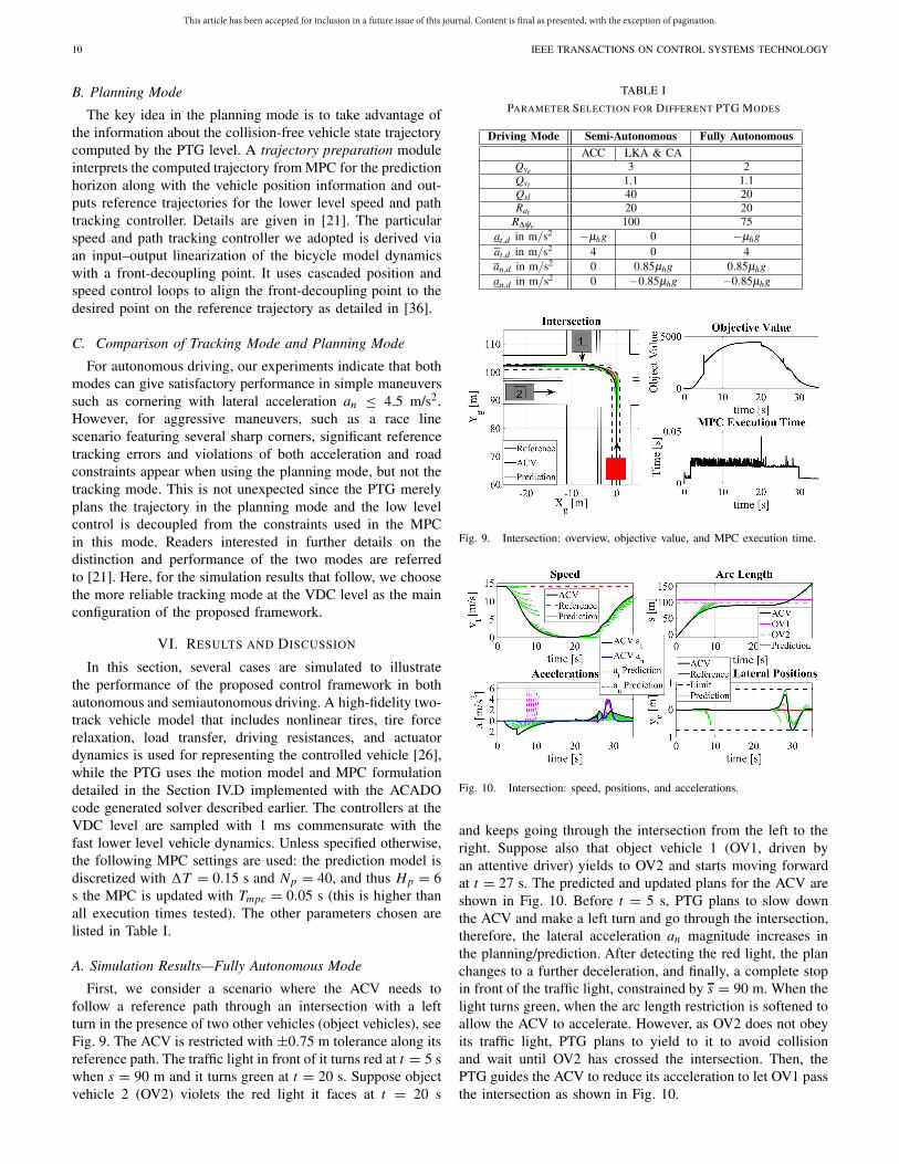
First, we consider a scenario where the ACV needs tofollow a reference path through an intersection with a leftturn in the presence of two other vehicles (object vehicles), seeFig. 9. The ACV is restricted with ±0.75 m tolerance along itsreference path. The traffic light in front of it turns red at t = 5 swhen s = 90 m and it turns green at t = 20 s. Suppose objectvehicle 2 (OV2) violets the red light it faces at t = 20 s

TABLE I

PARAMETER SELECTION FOR DIFFERENT PTG MODES

Fig. 9. Intersection: overview, objective value, and MPC execution time.

Fig. 10. Intersection: speed, positions, and accelerations.

and keeps going through the intersection from the left to theright. Suppose also that object vehicle 1 (OV1, driven byan attentive driver) yields to OV2 and starts moving forwardat t = 27 s. The predicted and updated plans for the ACV areshown in Fig. 10. Before t = 5 s, PTG plans to slow downthe ACV and make a left turn and go through the intersection,therefore, the lateral acceleration an magnitude increases inthe planning/prediction. After detecting the red light, the planchanges to a further deceleration, and finally, a complete stopin front of the traffic light, constrained by s = 90 m. When thelight turns green, when the arc length restriction is softened toallow the ACV to accelerate. However, as OV2 does not obeyits traffic light, PTG plans to yield to it to avoid collisionand wait until OV2 has crossed the intersection. Then, thePTG guides the ACV to reduce its acceleration to let OV1 passthe intersection as shown in Fig. 10.



Fig. 11. Passing with opposing traffic: overview, objective value, and MPCexecution time.

Fig. 12. Passing with opposing traffic: speed, positions, and accelerations.

The second set of results are generated for the ACV in aCA scenario involving two objects shown in Fig. 11: the staticOV1 partially occupies the same lane in front of the ACV.Another vehicle OV2 travels in the opposite direction on asecond lane. The ACV needs to pass the static OV1 to maintainthe reference speed, while avoiding collision with OV2. First,the PTG plans to reduce the speed and wait until OV2 on theleft lane has passed. However, when it approaches OV1 andobtain more information about the environment, the PTG findsit possible to pass OV1 before hitting OV2. Thus, it guidesthe ACV to accelerate, steer to the left to pass OV1 and, then,steer back to the reference lane to avoid OV2. For differentinitial conditions, the PTG could also force the ACV to waitfor OV2 to pass (for such a senario, see [20]).

B. Simulation Results—Semiautonomous Modes

To minimize acronyms in figures 13 and 14, we shall keepusing the notation ACV here, even though the operations aresemiautonomous. Fig. 13 shows results generated for drivingon a straight road in ACC mode with later control maintainedby the human driver. In this case, the PTG plans only thevehicle’s longitudinal acceleration at to track the referencespeed. When the speed of the front OV1 is lower than theACV, the ACV slows down and follows the front object at adistance defined by (25).

Fig. 14 shows results for the same maneuver conditionsbut with the PTG in LKA and CA semiautonomous modes.In these scenarios, the speed is held constant by the humandriver as the ACV approaches the slow moving vehicle in

Fig. 13. ACC mode: speed, positions, accelerations, and MPC executiontime.

Fig. 14. LKA&CA mode: lateral deviation, positions, accelerations, andMPC execution time.

TABLE II

EXECUTION TIME IN MILLISECONDS ON INTEL i5 4200U NOTEBOOK

CPU, 2.5 GHz, ESTIMATED BY THE ACADO SOLVER, Np = 40

front (see arc length). The PTG directs the ACV with lateralinput �ψp to pass OV1 in a safe distance of about 2 m untilthe ACV again tracks the reference with zero deviation. ThePTG makes the ACV pass on the left side of the object as thetraffic lane constraint prevents it from doing so on the rightside.

C. Execution Time of MPC

Table II shows the mean, minimum, and maximum exe-cution times estimated by the ACADO Toolbox for the pre-viously discussed maneuvers. It can be seen that the meanexecution times of different operation modes stay within therange of 11–16 ms. A closer examination of the executiontime records indicates that the execution time could jump to ahigher level when some inequality constraints become active.This is due to the active set method used in the solver wherethe Hessian matrix of the Lagrangian function needs to bereevaluated once the active constraints are updated. The jumpsare usually found when the speed starts decreasing becauseof obstacle/objects engaging in the inequality constraints.



Especially for the intersection case, a peak execution time ofabout 46.4 ms is observed when the traffic light turns greenand the constraint to avoid the red-light violating OV2 becomeactivated. The largest execution time can be used to guidethe selection of the update rate Tmpc of the MPC for real-time applications. While further investigation is required fora conclusive remark, these results indicate that the proposedframework for PTG is quite feasible for implementation onmodern real-time hardware.

VII. CONCLUSION

This paper presented a versatile PTG framework for fullyautonomous and semiautonomous vehicles feasible for real-time implementation. A nonlinear model of particle motiondescriptions and road references expressed in curvilinearFrenet frames is used in the PTG level to formulate and solvea nonlinear MPC problem. The formulation integrates severalreferences, obstacle descriptions, and hard constraints imposedby a traffic management or assigner module for lane limitsand traffic signal information, as well as vehicle dynamicsand actuation constraints. The control inputs computed at thePTG level can be utilized as control references by vehicledynamics control (VDC) level in tracking mode or merelytreated as planned optimal trajectories in planning modeby a suitable speed and path tracking VDC. A number ofsimulation results were included to illustrate the performanceof the PTG with VDC in tracking mode interfaced with ahigh-fidelity vehicle model for both fully autonomous andsemiautonomous modes in public traffic situations. It is shownthat the overall scheme shows good performance in variousscenarios with dynamic objects and operating modes. It isalso illustrated that the use of the particle motion model inthe PTG allows reasonable and practically feasible executiontimes, while handling active inequality constraints prevalentin dynamic public traffic scenarios. Future work will includeextensions of the predictive guidance framework to accom-modate uncertainties from environmental conditions, sensorimperfections, and other disturbances.

REFERENCES

[1] S. Karaman and E. Frazzoli, “Sampling-based algorithms for optimalmotion planning,” Int. J. Robot. Res., vol. 30, no. 7, pp. 846–894,Jun. 2011.

[2] E. Frazzoli, M. A. Dahleh, and E. Feron, “Maneuver-based motionplanning for nonlinear systems with symmetries,” IEEE Trans. Robot.,vol. 21, no. 6, pp. 1077–1091, Dec. 2005.

[3] A. Liniger and J. Lygeros, “A viability approach for fast recursivefeasible finite horizon path planning of autonomous RC cars,” in Proc.18th Int. Conf. Hybrid Syst., Comput. Control, New York, NY, USA,Apr. 2015, pp. 1–10.

[4] K. Kant and S. W. Zucker, “Toward efficient trajectory planning:The path-velocity decomposition,” Int. J. Robot. Res., vol. 5, no. 3,pp. 72–89, 1986.

[5] D. N. Godbole, V. Hagenmeyer, R. Sengupta, and D. Swaroop, “Designof emergency manoeuvres for automated highway system: Obstacleavoidance problem,” in Proc. 36th IEEE Conf. Decision Control, vol. 5.Dec. 1997, pp. 4774–4779.

[6] I. Papadimitriou and M. Tomizuka, “Fast lane changing computationsusing polynomials,” in Proc. Amer. Control Conf., vol. 1. Denver, CO,USA, Jun. 2003, pp. 48–53.

[7] F. Borrelli, D. Subramanian, A. U. Raghunathan, and L. T. Biegler,“MILP and NLP techniques for centralized trajectory planning of mul-tiple unmanned air vehicles,” in Proc. Amer. Control Conf., Minneapolis,MN, USA, Jun. 2006, pp. 5763–5768.

[8] Z. Shiller and J. C. Chen, “Optimal motion planning of autonomousvehicles in three dimensional terrains,” in Proc. IEEE Int. Conf. Robot.Autom., Cincinnati, OH, USA, May 1990, pp. 198–203.

[9] M. Vukov, A. Domahidi, H. J. Ferreau, M. Morari, and M. Diehl, “Auto-generated algorithms for nonlinear model predictive control on longand on short horizons,” in Proc. 52nd Conf. Decision Control (CDC),Dec. 2013, pp. 5113–5118.

[10] H. J. Ferreau, T. Kraus, M. Vukov, W. Saeys, and M. Diehl, “High-speed moving horizon estimation based on automatic code generation,”in Proc. 51st IEEE Conf. Decision Control (CDC), Maui, HI, USA,Dec. 2012, pp. 687–692.

[11] T. Keviczky, P. Falcone, F. Borrelli, and J. A. Hrovat, “Predictive controlapproach to autonomous vehicle steering,” in Proc. Amer. Control Conf.,Minneapolis, MN, USA, Jun. 2006, pp. 4670–4675.

[12] P. Falcone, F. Borrelli, J. Asgari, H. E. Tseng, and D. Hrovat, “Predictiveactive steering control for autonomous vehicle systems,” IEEE Trans.Control Syst. Technol., vol. 15, no. 3, pp. 566–580, May 2007.

[13] A. Gray, Y. Gao, J. K. Hedrick, and F. Borrelli, “Robust predictivecontrol for semi-autonomous vehicles with an uncertain driver model,”in Proc. IEEE Intell. Vehicles Symp., Gold Coast, Australia, Jun. 2013,pp. 208–213.

[14] Y. Gao, A. Gray, H. E. Tseng, and F. Borrelli, “A tube-based robust non-linear predictive control approach to semiautonomous ground vehicles,”Vehicle Syst. Dyn., vol. 52, no. 6, pp. 802–823, Apr. 2014.

[15] V. Turri, A. Carvalho, H. E. Tseng, K. H. Johansson, and F. Borrelli,“Linear model predictive control for lane keeping and obstacle avoidanceon low curvature roads,” in Proc. 16th Int. IEEE Annu. Conf. Intell.Transp. Syst., Hague, The Netherlands, Oct. 2013, pp. 378–383.

[16] A. Carvalho, Y. Gao, A. Gray, H. E. Tseng, and F. Borrelli, “Predictivecontrol of an autonomous ground vehicle using an iterative linearizationapproach,” in Proc. 16th Int. IEEE Annu. Conf. Intell. Transp. Syst.,Hague, The Netherlands, Oct. 2013, pp. 2335–2340.

[17] H. J. Ferreau, “Model predictive control algorithms for applications withmillisecond timescales,” Ph.D. dissertation, Arenberg Doctoral SchoolSci., KU Leuven, Leuven, Belgium, 2011.

[18] G. Prokop, “Modeling human vehicle driving by model predictive onlineoptimization,” Int. J. Vehicle Mech. Mobility, Vehicle Syst. Dyn., vol. 35,no. 1, pp. 19–53, 2001.

[19] P. Falcone, F. Borrelli, H. E. Tseng, J. Asgari, and D. Hrovat, “A hier-archical model predictive control framework for autonomous groundvehicles,” in Proc. Amer. Control Conf., Seattle, WA, USA, Jun. 2008,pp. 3719–3724.

[20] T. Weiskircher and B. Ayalew, “Predictive trajectory guidance for(semi-)autonomous vehicles in public traffic,” in Proc. Amer. ControlConf., Chicago, IL, USA, Jul. 2015, pp. 3328–3333.

[21] T. Weiskircher and B. Ayalew, “Frameworks for interfacing trajectorytracking with predictive trajectory guidance for autonomous road vehi-cles,” in Proc. Amer. Control Conf., Chicago, IL, USA, Jul. 2015,pp. 477–482.

[22] T. Weiskircher and B. Ayalew, “Predictive ADAS: A predictive trajectoryguidance scheme for advanced driver assistance in public traffic,” inProc. Eur. Control Conf., Linz, Austria, Jul. 2015, pp. 3402–3407.

[23] Q. Wang, T. Weiskircher, and B. Ayalew, “Hierarchical hybrid predictivecontrol of an autonomous road vehicle,” in Proc. Dyn. Syst. ControlConf., Columbus, OH, USA, 2015, p. V003T50A006.

[24] Q. Wang, B. Ayalew, and T. Weiskircher, “Optimal assigner decisionsin a hybrid predictive control of an autonomous vehicle in publictraffic,” in Proc. Amer. Control Conf., Boston, MA, USA, Jul. 2016,pp. 3468–3473.

[25] G. Genta, Motor Vehicle Dynamics: Modeling and Simulation (Serieson Advances in Mathematics for Applied Sciences), vol. 43. Singapore:World Scientific, 1997.

[26] B. Heissing and M. Ersoy, Eds., Chassis Handbook. Wiesbaden, Ger-many: Teubner, 2010.

[27] M. Abe and W. Manning, Vehicle Handling Dynamics: Theory Applica-tion. Amsterdam, The Netherlands: Butterworth-Heinemann, 2009.

[28] A. V. Zanten, R. Erhardt, and G. Pfaff, “VDC, the vehicle dynamicscontrol system of bosch,” SAE Tech. Paper 950759, 1995.

[29] A. V. Zanten, “Evolution of electronic control systems for improv-ing the vehicle dynamic behavior,” in Proc. Int. Symp. Adv. VehicleControl (AVEC), Hiroshima, Japan, 2002, pp. 1–9.

[30] V. Jain and T. Weiskircher, “Prediction–based hierarchical control frame-work for autonomous vehicles,” Int. J. Vehicle Auto. Syst., vol. 12, no. 4,pp. 307–333, 2014.

[31] J. L. Garriga and M. Soroush, “Model predictive control tuning methods:A review,” Ind. Eng. Chem. Res., vol. 8, no. 49, pp. 3505–3515, 2010.



[32] A. S. Yamashita, P. M. Alexandre, and A. C. Zanin, “Reference trajec-tory tuning of model predictive control,” Control Eng. Pract., no. 50,pp. 1–11, May 2016.

[33] P. Stolze, M. Kramkowski, T. Mouton, M. Tomlinson, and R. Ken-nel, “Increasing the performance of finite-set model predictive controlby oversampling,” in Proc. IEEE Int. Conf. Ind. Technol. (ICIT),Cape Town, South Africa, Feb. 2013, pp. 551–556.

[34] R. Quirynen, M. Vukov, M. Zanon, and M. Diehl, “Autogeneratingmicrosecond solvers for nonlinear mpc: A tutorial using acado inte-grators,” Optim. Control Appl. Methods, vol. 36, pp. 685–704, 2015.

[35] H. F. Grip, L. Imsland, T. A. Johansen, J. C. Kalkkuhl, and A. Suissa,“Vehicle sideslip estimation,” IEEE Control Syst., vol. 29, no. 5,pp. 36–52, Oct. 2009.

[36] D. Heß, M. Althoff, and T. Sattel, “Comparison of trajectory trackingcontrollers for emergency situations,” in Proc. IEEE Intell. Veh. Symp.,Gold Coast, Australia, Jun. 2013, pp. 163–170.

Thomas Weiskircher received the Diploma degreein mechatronics engineering from the Universitätdes Saarlandes, Saarbrücken, Germany, in 2009,and the Ph.D. degree in mechanical engineeringfrom Technische Universität Kaiserslautern, Kaiser-slautern, Germany, in 2013.

Since 2014, he has been a Post-DoctoralResearcher in vehicle control with the AppliedDynamics and Control Research Group, Clem-son University International Center of AutomotiveResearch, Greenville, SA, USA. His current research

interests include optimal control, real-time model predictive control forautomotive applications, vehicle dynamics control, and active safety systems.

Qian Wang received the Diploma and master’sdegrees in vehicle engineering from the South ChinaUniversity of Technology, Guangzhou, China, in2010 and 2013, respectively. He is currently pur-suing the Ph.D. degree with the Applied Dynamicsand Control Research Group, Clemson University,Clemson, SC, USA.

His current research interests include optimal con-trol, predictive motion planning for autonomousvehicles, and control allocation for vehicle actuationsystem.

Beshah Ayalew received the M.S. and Ph.D. degreesin mechanical engineering from Pennsylvania StateUniversity, State College, PA, USA, in 2005.

He is currently a Professor of Automotive Engi-neering, and the Director of the DOE GATE Cen-ter of Excellence in Sustainable Vehicle Systems,Clemson University International Center for Auto-motive Research, Greenville, SA, USA. His currentresearch interests include the modeling and controlof dynamic systems with applications in vehiclesystems dynamics, manufacturing processes, and

vehicle energy systems. His recent research is funded by various federal andindustry grants and contracts.

Dr. Ayalew is an active member of the ASMEs Vehicle Design Committee,the IEEE Control Systems Society, and Society of Automotive Engineers(SAE). He received the Ralph R. Teetor Award from SAE in 2014, theClemson University Board of Trustees Award for Faculty Excellence in 2012,the NSF CAREER Award in 2011, and the Penn State Alumni AssociationDissertation Award in 2005.

Date post:	11-Mar-2018
Category:	Documents
Upload:	trantuong
View:	222 times
Download:	1 times

IEEE TRANSACTIONS ON CONTROL SYSTEMS … Systems Dynamics... · the framework is a nonlinear model...

Documents