IEEE TRANSACTIONS ON IMAGE PROCESSING, …vmp93/Journal_pub/DASHN_TIP_revised_final.pdfIEEE...

IEEE TRANSACTIONS ON IMAGE PROCESSING, VOL. X, NO. X, MONTH 20XX 1

DASH-N: Joint Hierarchical DomainAdaptation and Feature Learning

Hien V. Nguyen†, Member, IEEE, Huy Tho Ho†, Member, IEEE, Vishal M. Patel, Member, IEEE, andRama Chellappa, Fellow, IEEE

Abstract—Complex visual data contain discriminative struc-tures that are difficult to be fully captured by any single featuredescriptor. While recent work on domain adaptation focuseson adapting a single hand-crafted feature, it is important toperform adaptation on a hierarchy of features to exploit therichness of visual data. We propose a novel framework fordomain adaptation using a sparse and hierarchical network(DASH-N). Our method jointly learns a hierarchy of featurestogether with transformations that rectify the mismatch betweendifferent domains. The building block of DASH-N is the latentsparse representation. It employs a dimensionality reduction stepthat can prevent the data dimension from increasing too fast asone traverses deeper into the hierarchy. Experimental resultsshow that our method compares favorably with competing state-of-the-art methods. In addition, it is shown that a multi-layerDASH-N performs better than a single-layer DASH-N.

Index Terms—Domain adaptation, hierarchical sparse repre-sentation, dictionary learning, object recognition.

I. INTRODUCTION

In many practical computer vision applications, we are oftenconfronted with the situation where the data that we use totrain classification/regression algorithm has a different distri-bution or representation with that presented during testing. Theubiquity of this problem is well-known to machine learningand computer vision researchers. This challenge is commonlyreferred to as covariate shift [1], or class imbalance [2].For instance, indoor images are quite different from outdoorimages, just as videos captured with a high definition cameraare from those collected using a webcam. This detrimentaleffect is often a dominant factor contributing to the poorperformances of many computer vision algorithms. As anexample of the effect of distribution mismatch, Ben-David etal. [3] show that, under certain assumption, the bound on thetest error linearly increases with the `1 divergence betweentraining and testing distributions. Even worse, data from thetest domain are often scarce and expensive to obtain. Thismakes it impractical to re-train an algorithm from scratchsince a learning algorithm would generalize poorly when an

†: Authors contributed equally.Hien V. Nguyen is a research scientist at Siemens Corporate Technology

in Princeton, NJ. e-mail: [email protected] Tho Ho is with the Department of Electrical Engineering and the

Center for Automation Research, UMIACS, University of Maryland, CollegePark, MD 20742 USA e-mail: [email protected]

Vishal M. Patel is with the department of Electrical and Computer Engineer-ing at Rutgers University, Piscataway, NJ USA [email protected].

Rama Chellappa is with the Department of Electrical Engineering and theCenter for Automation Research, UMIACS, University of Maryland, CollegePark, MD 20742 USA e-mail: [email protected].

insufficient amount of data is presented [4]. Regardless of thecause, any distributional change that may occur after trainingcan degrade the performance of the system when it comesto testing. Domain adaptation also known as domain-transferlearning attempts to minimize this degradation.

The problems caused by domain changes have receivedsubstantial attention in recent years. The problem can beinformally stated as follows. Given a source domain whoserepresentation or distribution can be different from that of thetarget domain, how to effectively utilize the model trainedon the source data to achieve a good performance on thetarget data. It is also often assumed that the source domainhas sufficient labelled training samples while there are onlya few (both labelled and unlabelled) samples available in thetarget domain. It has been shown in [5]–[9] that domain adap-tation techniques can significantly improve the performanceof computer vision tasks such as visual object detection andrecognition.

Most of the algorithms for adapting a recognition system toa new visual domain share a common architecture containingtwo main stages. First, features are extracted separately forsource and target using hand-crafted feature descriptors, fol-lowed by the second stage where transformations are learnedin order to rectify the discrepancy between the two domains.This architecture has several drawbacks. Without any knowl-edge about the target domain, the feature extraction performedon the source data can ignore information important to thetarget data. In addition, the process of designing features, suchas SIFT [10] or SURF [11], is tedious and time-consuming. Itrequires a deep understanding and a careful examination of theunderlying physics that governs the generation of data. Suchrequirements might be impractical given that the data from thetarget domain are often very scarce.

Another issue is that discriminative information can beembedded in multiple levels of the features hierarchy. High-level features are sometimes more useful than low-level ones.In fact, this is one of the main motivations behind thedevelopment of hierarchical networks (e.g. [12], [13]) so thatmore complex abstraction from a visual object can be captured.The traditional framework of domain adaptation employs ashallow architecture containing a single layer. This ignoresthe possibility of transferring at multiple levels of the featurehierarchy. In this paper, we show that jointly learning ahierarchy of features could significantly improve the accuracyof cross-domain classification. We compare and contrast ourapproach with recent work on using deep networks in domainadaptation. Our method uses the latent sparse representation.


The network incorporates a dimensionality reduction stage toprevent the feature dimension from increasing too fast as onetraverses deeper into the hierarchy. The contributions of ourpaper is summarized below.

Contributions: In order to address the limitations of ex-isting approaches, we propose a novel approach for domainadaptation that possesses the following advantages:• Adaptation is performed on multiple levels of the feature

hierarchy in order to maximize the knowledge transfer.The hierarchical structure allows the transfer of usefulinformation that might not be well captured by existingdomain adaptation techniques.

• Adaptation is done jointly with feature learning. Ourmethod learns a hierarchy of sparse codes and uses themto describe a visual object instead of relying on any low-level feature.

• Unlike existing hierarchical networks, our network ismore computationally efficient with a mechanism toprevent the data dimension from increasing too fast asthe number of layer increases.

We provide extensive experiments to show that our approachperforms better than many current state-of-the-art domainadaptation methods. This is interesting since in our method,training is entirely generative followed by a linear support vec-tor machine while several other methods employ discrimina-tive training together with non-linear kernels. Furthermore, weintroduce a new set of data for benchmarking the performanceof our algorithm. The new dataset has two domains containinghalf-toned and edge images, respectively. In order to facilitatefuture research in the area, a Matlab implementation of ourmethod will be made available.

A. Organization of the paper

This paper is organized as follows. Related works ondomain adaptation are discussed in Section II. The mainformulation of DASH-N is given in Section III, followed bythe optimization procedure in Section V. Experimental resultson domain adaptation for object recognition are presented inSection VI. Finally, Section VII concludes the paper with abrief summary and discussion.

II. RELATED WORKS

In this section, we review some related works on domainadaptation and hierarchical feature learning.

A. Domain Adaptation

While domain adaptation was first investigated in speechand natural language processing [14]–[16], it has been studiedextensively in other areas such as machine learning [3], [17]and computer vision, especially in the context of visual objectrecognition [5]–[9], [18]. Domain adaptation for visual recog-nition was introduced by Saenko et al. [5] in a semi-supervisedsetting. They employed metric learning to learn the domainshift using partially labeled data from the target domain. Thiswork was extended by Kulis et al. [6] to handle asymmetric

domain transformations. Gopalan et al. [7] addressed theproblem of unsupervised domain adaptation, where samplesfrom the target domain are unlabeled, by using an incrementalapproach based on Grassmann manifolds. By formulating ageodesic flow kernel, Gong et al. [8] and Zheng et al. [19]independently extended the idea of interpolation to integratean infinite number of subspaces on the geodesic flow from thesource domain to the target domain. Chen et al. [20] presenteda co-training based method that slowly adapted a training setfrom the source to the target domain. An information-theoreticmethod for unsupervised domain adaptation was proposed byShi and Sha [21] that attempted to find a common featurespace, where the source and target data distributions are similarand the misclassification error is minimized.

Sparse representation and dictionary-based methods for do-main adaptation [22]–[24] are also gaining a lot of traction. Inparticular, [22] modeled dictionaries across different domainswith a parametric mapping function, while [24] enforceddifferent domains to have a common sparse representation onsome latent domain. Another class of techniques [25], [26]performed domain adaptation by directly learning a targetclassifier using classifiers trained on the source domain(s).

A major drawback of some of the existing approaches isthat the domain shifting transformation is considered onlyat a single layer and may not capture adequately the shiftbetween the source and target domain. It is worth noting thatalthough [27] also named their method hierarchical domainadaptation, the paper is not related to ours. They made useof hierarchical Bayesian prior, while we employ a multi-layernetwork of sparse representation.

There are also some closely related machine learning prob-lems that have been studied extensively, including transferlearning or multi-task learning [28], self-taught learning [29],semi-supervised learning [30] and multiview analysis [31]. Areview of domain adaptation methods from machine learningand the natural language processing communities can be foundin [32]. A survey on the related field of transfer learning canbe found in [33].

B. Hierarchical Feature Learning

Designing features for visual objects is a time-consumingand challenging task that requires a deep understanding of do-main knowledge. It is also non-trivial to adapt these manuallydesigned features to new types of data such as hyperspectral orrange-scan images. For this reason, learning features from theraw data has become increasingly popular with demonstratedcompetitive performances on practical computer vision tasks[12], [13], [34]. In order to capture the richness of data, amulti-layer or hierarchical network is employed to learn aspectrum of features, layer by layer.

The design of multi-layer networks has been an activeresearch topic in computer vision. One of the early worksincludes [35], which used a multistage system to extract salientfeatures in the image at different spatial scales. By learninghigher-level feature representations from unlabelled data, deepbelief networks (DBN) [12] and its variants, such as convo-lutional DBNs [13] and deep autoencoders [36], have been


shown to be effective when applied to classification problems.Motivated by recent works on deep learning, multi-layer sparsecoding networks [34], [37], [38] have been proposed to buildfeature hierarchies layer by layer using sparse codes andspatial pooling. Each layer in these networks contains a codingstep and a pooling step. A dictionary is learned at each codingstep which then serves as a codebook for obtaining sparsecodes from image patches or pooled features. Spatial poolingschemes, most notably max-pooling, group the sparse codesfrom adjacent blocks into common entities. This operationmakes the resulting features more invariant to certain changescaused by translation and rotation. The pooled sparse codesfrom one layer serve as the input to the next layer.

Although the high dimension of the feature vectors obtainedfrom a hierarchical network may provide some improvementsin classification tasks [12], [13], [34], it may also lead to highredundancy and thus, reduce the efficiency of these algorithms.As a result, it is desirable to have a built-in mechanism inthe hierarchy to reduce the dimension of the feature vectorswhile keeping their discriminative power. Hierarchical featurelearning has also been used in domain adaptation such as in[39], [40].

Deep learning has recently made significant improvementto cross-domain classification [39]–[43]. One of the earlyworks [39] uses stacked auto-encoder (SDA) to learn high-level features in an unsupervised manner. They show thatdeep features improve sentiment classification accuracy ona dataset of 22 different domains. A fast variant of auto-encoder [40] was developed to make SDA training two ordersof magnitudes faster than that of the traditional counterpart.Another architecture [44] was based on CNN to learn genericfeatures from a large dataset containing millions of images ofover 1000 classes. This work was able to bring down the state-of-the-art error on ImageNet dataset from 26.1% to 15.3%. Inaddition, the learned features have been shown to generalizewell across different domains [41], [42], making them suit-able for domain adaptation. The effectiveness of the learnedfeatures can be attributed to the large number of trainingimages which probably contains significant information fromall interested domains. Another work [43] also makes use ofCNN to learn features but with an interesting twist inspired bythe work of [7]. In particular, they creates a path of interpolatedrepresentations by slowly varying the sampling proportion ofsource and target data. Each representation along the path isgenerated by applying CNN on the resulting dataset.

Additional data greatly benefit the performance of domainadaptation algorithm. For example, [42] showed that the cross-domain classification accuracies on several popular datasets[5], [45] can be improved by employing a large number oftraining images from other sources. The improvement can beattributed to the high-capacity learning framework of deepnetwork like CNN. It might also be because the learner hasseen sufficient information for different domains from the largenumber of additional training images. It is understandable thatthis approach requires a lot of data to perform well. However,data collection is difficult in many practical applications.For instance, medical data are rarely available in abundancelike RGB images. For this reason, our paper will focus on

comparing with those methods that do not use additional datafrom external sources.

III. BACKGROUND

Since our formulation is based on sparse coding and dic-tionary learning, in this section, we briefly give a backgroundon these topics.

A. Dictionary Learning

Given a set of training samples Y = [y1, . . . ,yn] ∈ Rd×n,the problem of learning a dictionary together with the sparsecodes is typically posed as the minimization of the followingcost function over (D, X):

‖Y −DX‖2F +βΨ(X) s.t. ‖di‖2= 1,∀i ∈ [1,K] (1)

where ‖Y‖F denotes the Frobenius norm defined as ‖Y‖F =√∑i,j |Yi,j |2, D = [d1, . . . ,dK ] ∈ Rd×K is the sought

dictionary, X = [x1, . . . ,xn] ∈ RK×n is the horizontalconcatenation of sparse codes, β is a non-negative constantand Ψ promotes sparsity. Various methods have been proposedin the literature for solving such optimization problem. In thecase when `0 norm is enforced, the K-SVD [46] algorithm canbe used to train a dictionary. One can also promote sparsityby enforcing the `1 norm on X. In this case, one can use thealgorithm proposed in [47] to solve the above problem. See[46] and [47] for more details.

B. Latent Sparse Representation

From the observation that signals often lie on a low-dimensional manifold, several authors have proposed toperform dictionary learning and sparse coding in a latentspace [48]–[50]. We call it latent sparse representation todistinguish from the formulation in (1). This is done byminimizing the following cost function over (P, D, X):

L(Y,P,D,X, α, β) =

‖PY −DX‖2F +α‖Y −PTPY‖2F +β‖X‖1s.t. PPT = I and ‖di‖2= 1, ∀i ∈ [1,K], (2)

where P ∈ Rp×d is a linear transformation that brings thedata to a low-dimensional feature space (p < d). Note that thedictionary is now in the low-dimensional space D ∈ Rp×K .The first term of the cost function promotes sparsity of signalsin the reduced space. The second term is the amount of energydiscarded by the transformation P, or the difference betweenlow-dimensional approximations and the original signals. Theminimization of the second term encourages the learned trans-formation to preserve the useful information present in theoriginal signals. Besides the computational advantage, [49]shows that this optimization can recover the underlying sparserepresentation better than the traditional dictionary learningmethods. This formulation is attractive since it allows thetransformation of the data into another domain to betterhandle different sources of variation such as illumination andgeometric articulation.


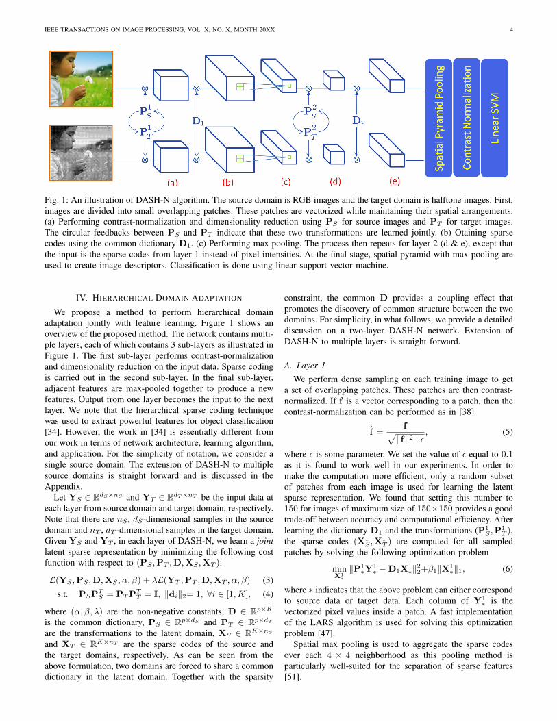
Fig. 1: An illustration of DASH-N algorithm. The source domain is RGB images and the target domain is halftone images. First,images are divided into small overlapping patches. These patches are vectorized while maintaining their spatial arrangements.(a) Performing contrast-normalization and dimensionality reduction using PS for source images and PT for target images.The circular feedbacks between PS and PT indicate that these two transformations are learned jointly. (b) Otaining sparsecodes using the common dictionary D1. (c) Performing max pooling. The process then repeats for layer 2 (d & e), except thatthe input is the sparse codes from layer 1 instead of pixel intensities. At the final stage, spatial pyramid with max pooling areused to create image descriptors. Classification is done using linear support vector machine.

IV. HIERARCHICAL DOMAIN ADAPTATION

We propose a method to perform hierarchical domainadaptation jointly with feature learning. Figure 1 shows anoverview of the proposed method. The network contains multi-ple layers, each of which contains 3 sub-layers as illustrated inFigure 1. The first sub-layer performs contrast-normalizationand dimensionality reduction on the input data. Sparse codingis carried out in the second sub-layer. In the final sub-layer,adjacent features are max-pooled together to produce a newfeatures. Output from one layer becomes the input to the nextlayer. We note that the hierarchical sparse coding techniquewas used to extract powerful features for object classification[34]. However, the work in [34] is essentially different fromour work in terms of network architecture, learning algorithm,and application. For the simplicity of notation, we consider asingle source domain. The extension of DASH-N to multiplesource domains is straight forward and is discussed in theAppendix.

Let YS ∈ RdS×nS and YT ∈ RdT×nT be the input data ateach layer from source domain and target domain, respectively.Note that there are nS , dS-dimensional samples in the sourcedomain and nT , dT -dimensional samples in the target domain.Given YS and YT , in each layer of DASH-N, we learn a jointlatent sparse representation by minimizing the following costfunction with respect to (PS ,PT ,D,XS ,XT ):

L(YS ,PS ,D,XS , α, β) + λL(YT ,PT ,D,XT , α, β) (3)

s.t. PSPTS = PTPT

T = I, ‖di‖2= 1, ∀i ∈ [1,K], (4)

where (α, β, λ) are the non-negative constants, D ∈ Rp×K

is the common dictionary, PS ∈ Rp×dS and PT ∈ Rp×dT

are the transformations to the latent domain, XS ∈ RK×nS

and XT ∈ RK×nT are the sparse codes of the source andthe target domains, respectively. As can be seen from theabove formulation, two domains are forced to share a commondictionary in the latent domain. Together with the sparsity

constraint, the common D provides a coupling effect thatpromotes the discovery of common structure between the twodomains. For simplicity, in what follows, we provide a detaileddiscussion on a two-layer DASH-N network. Extension ofDASH-N to multiple layers is straight forward.

A. Layer 1

We perform dense sampling on each training image to geta set of overlapping patches. These patches are then contrast-normalized. If f is a vector corresponding to a patch, then thecontrast-normalization can be performed as in [38]

f =f√‖f‖2+ε

, (5)

where ε is some parameter. We set the value of ε equal to 0.1as it is found to work well in our experiments. In order tomake the computation more efficient, only a random subsetof patches from each image is used for learning the latentsparse representation. We found that setting this number to150 for images of maximum size of 150×150 provides a goodtrade-off between accuracy and computational efficiency. Afterlearning the dictionary D1 and the transformations (P1

S ,P1T ),

the sparse codes (X1S ,X

1T ) are computed for all sampled

patches by solving the following optimization problem

minX1

∗

‖P1∗Y

1∗ −D1X

1∗‖22+β1‖X1

∗‖1, (6)

where ∗ indicates that the above problem can either correspondto source data or target data. Each column of Y1

∗ is thevectorized pixel values inside a patch. A fast implementationof the LARS algorithm is used for solving this optimizationproblem [47].

Spatial max pooling is used to aggregate the sparse codesover each 4 × 4 neighborhood as this pooling method isparticularly well-suited for the separation of sparse features[51].


B. Layer 2

In this layer, we perform similar computations except thatthe input is the sparse codes from layer 1 instead of imagepixels. The features obtained from the previous layer areaggregated by concatenation over each 4 × 4 neighborhoodand contrast-normalized. This results in a new representationthat is more robust to occlusion and illumination. Similar tolayer 1, we also randomly sample 150 normalized featurevectors f from each image for training. `1 optimization isagain employed to compute the sparse codes of the normalizedfeatures f .

At the end of layer 2, the sparse codes are then aggre-gated using max pooling in a multi-level patch decomposition(i.e. spatial pyramid max pooling). At level 0 of the spatialpyramid, a single feature vector is obtained by performingmax pooling over the whole image. At level 1, the image isdivided into four quadrants and max pooling is applied to eachquadrant, yielding 4 feature vectors. Similarly, for level 2, weobtain 9 feature vectors, and so on. In this paper, max poolingusing a three level spatial pyramid is used. As a result, the finalfeature vector returned by the second layer for each image isa result of concatenating 14 feature vectors from the spatialpyramid.

V. OPTIMIZATION PROCEDURE

In this section, we describe how the cost function in (3) isminimized. First, let us define

KS = YTS YS , KT = YT

T YT , K =

(KS 0

0√λKT

)(7)

to be the Gram matrix of source, target, and their blockdiagonal concatenation, respectively. It can be shown that (seethe Appendix) the optimal solution of (3) takes the followingform

D = [ATSKS ,

√λAT

TKT ]B (8)

PS = (YSAS)T , PT = (YTAT )T , (9)

for some AS ∈ RnS×p, AT ∈ RnT×p and B ∈ R(nS+nT )×K .Notice that rows of each transformation live in the columnsubspace of the data from its own domain. In contrast, columnsof the dictionary are jointly created by the data of both sourceand target.

A. Solving for (AS ,AT )

The orthogonal constraint in (4) can be re-written using (9)as

ATSKSAS = I, AT

TKTAT = I. (10)

By substituting (9), (8) into (3) and making use of theorthogonal constraint in (10), the formulation can be simplifiedas follows (see derivation in the Appendix)

minG

tr(GTHG) s.t. GTSGS = GT

TGTT = I, (11)

where H is defined as

H = Λ12 VTK((I−BX)(I−BX)T − αI)KVΛ

12 , (12)

V =

(VS 00 VT

), Λ =

(ΛS 0

0√λΛT

), (13)

KS = VSΛSVTS , KT = VTΛTVT

T . (14)

Here (14) is given by the eigen-decompositions of the Grammatrices. Finally, G is defined as

G = [GS ,√λGT ], (15)

GS = Λ12

SVTSAS , GT = Λ

12

TVTT AT . (16)

The optimization in (11) is non-convex due to the orthogonal-ity constraints. However, G can be learned efficiently usingthe algorithm proposed by [52]. Given G, the solution of(AS ,AT ) is simply given by

AS = VSΛ− 1

2

S GS , AT = VTΛ− 1

2

T GT . (17)

We note that the optimization step involves the eigen-decompositions of large Gram matrices whose dimensionsequal to the number of training samples (≈ 105 in ourexperiments). This is computationally infeasible. We propose aremedy for this. The source is taken for the illustration purposeand the computation for the target is similar. First, we computethe eigen-decomposition of the following matrix

CS = YSYTS = USΛ′SUT

S ∈ RdS×dS . (18)

Then, the dS dominant eigenvectors of KS can be recoveredas

VS = YTS USΛ′S

− 12 . (19)

The relationship in (19) between VS and US can be easilyverified using an SVD-decomposition of YS .

The signal dimension dS is much smaller than the numberof training samples nS in our experiments (e.g. 103 versus105). The eigen-decomposition of CS is therefore much moreefficient than that of KS . Finally, non-zero eigenvalues in ΛS

are given by the diagonal coefficients of Λ′S .

B. Solving for (B,X)

If we fix (AS ,AT ), then learning (B,XS ,XT ) can be doneusing any dictionary learning algorithm. In order to see this,let us define

Z = [ASKS ,√λATKT ], (20)

X = [XS ,√λXT ]. (21)

The cost function can be re-written in a familiar form asfollows

‖Z−DX‖2F +β(‖XS‖1+λ‖XT ‖1). (22)

We use the LASSO to solve for the sparse codes X and theefficient online dictionary learning algorithm [47] to solve forD. The solution of B can be recovered, using the relationshipin (8), simply by

B = Z†D,


TABLE I: Recognition rates of different approaches on four domains (C: Caltech, A: Amazon, D: DSLR, W: Webcam). 10common classes are used. Red color denotes the best recognition rates. Blue color denotes the second best recognition rates.

Method C → A C → D A → C A → W W → C W → A D → A D → WMetric [5] 33.7± 0.8 35.0± 1.1 27.3± 0.7 36.0± 1.0 21.7± 0.5 32.3± 0.8 30.3± 0.8 55.6± 0.7SGF [7] 40.2± 0.7 36.6± 0.8 37.7± 0.5 37.9± 0.7 29.2± 0.7 38.2± 0.6 39.2± 0.7 69.5± 0.9

GFK (PLS+PCA) [8] 46.1± 0.6 55.0± 0.9 39.6± 0.4 56.9± 1.0 32.8± 0.1 46.2± 0.6 46.2± 0.6 80.2± 0.4SDDL [24] 49.5± 2.6 76.7± 3.9 27.4± 2.4 72.0± 4.8 29.7± 1.9 49.4± 2.1 48.9± 3.8 72.6± 2.1HMP [34] 67.7± 2.3 70.2± 5.1 51.7± 4.3 70.0± 4.2 46.8± 2.1 61.5± 3.8 64.7± 2.0 76.0± 4.0

DASH-N (1st layer) 60.3± 2.7 79.6± 3.1 52.2± 2.1 74.1± 4.6 45.31± 3.7 68.7± 2.9 65.9± 2.1 76.3± 2.3DASH-N (1st+2nd layers) 71.6± 2.2 81.4± 3.5 54.9± 1.8 75.5± 4.2 50.2± 3.3 70.4± 3.2 68.9± 2.9 77.1± 2.8

(a) Amazon (b) Caltech (c) DSLR (d) Webcam

Fig. 2: Example images from the LAPTOP-101 class indifferent domains. First row: original images, second row:halftone images, third row: edge images.

where † denotes the MoorePenrose pseudo-inverse.It is straight forward to extend the above formulation

to handle the case of multiple source domains. Details ofderivation for this case are included in the Appendix.

VI. EXPERIMENTS

The proposed algorithm is evaluated in the context ofobject recognition using a recent domain adaptation dataset[5], containing 31 classes, with the addition of imagesfrom the Caltech-256 dataset [45]. There are 10 commonclasses between the two datasets (BACKPACK, TOURING-BIKE, CALCULATOR, HEADPHONES, COMPUTER-KEYBOARD, LAPTOP-101, COMPUTER-MONITOR,COMPUTER-MOUSE, COFFEE-MUG, and VIDEO-PROJECTOR) which contain a total of 2533 images. Domainshifts are caused by variations in factors such as pose, lighting,resolution, etc., between images in different domains. Figure2 shows example images from the LAPTOP-101 class withrespect to different domains. We compare our method withstate-of-the-art adaptation algorithms such as [5], [7], [8],[24]. Baseline results obtained using the hierarchical featurelearning in [34] by learning the dictionaries separately forthe source and target domains without performing domainadaptation are also included. Furthermore, in order to betterassess the ability to adapt to a wide range of domains,experimental results are also reported on new imagesobtained by performing halftoning [53] and edge detection[54] algorithms on images from the datasets in [5], [45].

A. Experiment Setup

We follow the experimental set-ups of [8]. The results using10 as well as 31 common classes are reported. In both cases,experiments are performed in 20 random trials for each pair ofsource and target domains. If the source domain is Amazonor Caltech, 20 samples are used in the training. Otherwise,only 8 training samples are used for DLSR and Webcam. Thenumber of target training samples is always set equal to 3.The remaining images from the target domain in each splitare used for testing.

B. Parameter Settings

In our experiments, all images are resized to be no largerthan 150×150 with preserved ratio and converted to grayscale.The patch size is set equal to 5 × 5. The parameter λ is setequal to 4 in order to account for less training samples fromthe target than that from the source, and α is set equal to1.5 for all experiments. We also found that using βtrain =0.3 for training and βtest = 0.15 for testing yields the bestperformance. The same values for these parameters are usedfor both the first and second layer. A smaller sparsity constantoften makes the decoding more stable, thus, leads to moreconsistent sparse codes. This is similar to the finding in [34].The number of dictionary atoms is set equal to 200 and 1500in the first and second layer, respectively. The dimension ofthe latent domain is set equal to 20 and 750 in the first andsecond layer, respectively. It is worth noting that the inputfeature to layer 2 has the dimension of 3200. This results fromaggregating sparse codes obtained from the first layer over a4×4 spatial cell (4×4×200). By projecting them onto a latentdomain of dimension of 750, the computations become moretractable. A three level spatial pyramid, partitioned into 1×1,2×2, and 3×3, is used to perform the max pooling in the finallayer. Linear SVM [55] with the regularization parameter of10 is employed for classification. It is worth noting that we donot use any part of the testing data in tuning the algorithmicparameters. The sparsity constants such as α, βtrain and βtestare set to the standard values used by many popular sparselearning softwares such as SPAMS [47] and ScSPM [56]. Forparameters such as patch size, dictionary size, latent spacedimensions and the linear SVM regularization parameter, thefindings in [34], [46], [49] are employed to create a smallsubset of values and cross-validation on the training data isperformed to obtain the optimal settings.


0 50 100 150 200 2500

0.002

0.004

0.006

0.008

0.01

0.012

0.014X = 43Y = 0.0119

Atom number

Re

sp

on

se

Training data for BACKPACK

X = 103Y = 0.0123

X = 136Y = 0.0113

X = 160Y = 0.0108

0 50 100 150 200 2500

0.002

0.004

0.006

0.008

0.01

0.012

0.014

X = 43Y = 0.0101

Atom number

Re

sp

on

se

Test data for BACKPACK

X = 103Y = 0.0126

X = 136Y = 0.0112

X = 160Y = 0.0106

Fig. 3: Dictionary responses of training (left) and testing (right) data for the BACKPACK class for the pair DSLR-Webcamdomains in the first layer.

C. Computation Time

It takes an average of 35 minutes to perform the dictionarylearning and feature extraction of all training samples usingour Matlab implementation on a computer with a 3.8 GHzIntel i7 processor. It takes less than 2 seconds to compute thefeature for a test image of size 150 × 150 using both layersof the hierarchy.

D. Object Recognition

1) 10 Common Classes: The recognition results of differentalgorithms on 8 pairs of source-target domains are shown inTable I. It can be seen that DASH-N outperforms all comparedmethods in 7 out of 8 pairs of source-target domains. Forpairs such as Caltech-Amazon, Webcam-Amazon, or DSLR-Amazon, we achieve more than 20% improvements overthe next best algorithm without feature learning used in thecomparison (from 49.5% to 71.6%, 49.4% to 70.4%, and48.9% to 68.9%, respectively). It is worth noting that whilewe employ a generative approach for learning the feature, ourmethod consistently achieves better performance than [24],which uses discriminative training together with non-linearkernels. It is also clear from the table that the multi-layerDASH-N outperforms the single-layer DASH-N. In the caseof adapting from Caltech to Amazon, the performance gainby using a combination of features obtained from both layersrather than just features from the first layer is more than 10%(from 60.3% to 71.6%).

The results obtained by using Hierarchical Matching Pursuit(HMP) [34], without performing domain adaptation, are alsoincluded in the comparison in order to better evaluate theimprovements provided by the proposed approach. In order toextract features using HMP, a dictionary is learned separatelyper the source and target domains in each layer. Sparse codesfor data from the source and target domains are then computedusing the corresponding dictionary. Similar to our approach,the classification is performed using the concatenated featuresobtained a two-layer network. HMP parameters are selected

using cross-validation on the training data. It can be seen fromTable I that, although HMP does not perform as well as theproposed method, it achieves reasonably good performance onthe dataset. In many cases, it even outperforms other domainadaptation methods used in the comparison. This demonstratesthe effectiveness of learning feature representation. However,it is also clear from the table that by learning a commonrepresentation at each layer of the hierarchy, our algorithmis able to capture the domain shift better. As a result, itconsistently achieves better classification rates compare toHMP in all scenarios.

In order to illustrate the encoding of features using thelearned dictionary in the first layer, Figure 3 shows theresponses of the training and testing data for the BACKPACKclass with respect to each atom of the dictionary in the firstlayer for the pair DSLR-Webcam domains. The sparse codesfor all the patches of the training and testing images belong tothe class are computed. The absolutes of these sparse vectorsare summed together and normalized to unit length. Smallcomponents of the normalized sparse codes are thresholdedto better show the correspondences between the training andtesting data. It can be seen from the figure that the sparse codesfor the training and testing data for the BACKPACK class bothhave high responses in four different dictionary atoms (43,103, 136 and 160).

2) 31 Classes and Multiple Sources: We also compare therecognition results for all 31 classes between our approachand other methods in both cases of single (Table II) andmultiple source domains (Table III). It can be seen fromTables II and III that our results, even using only featuresextracted from the first layer, are consistently better than thatof other algorithms in all the domain settings, except the resultsobtained by using features extracted from deep networks [42],[43]. This proves the effectiveness of the feature learningprocess using latent sparse representation. It is worth notingthat the deep convolutional network used in [42] is trainedin a fully supervised fashion for more than a week usinga very large external dataset, called ImageNet [59], which


5 10 15 20 2570

72

74

76

78

80

82

84

Dimension

Recognitio

n r

ate

(%

)

Amazon−DSLR

Caltech−Webcam

Webcam−DSLR

(a) First layer

250 500 750 1000 1250 150072

74

76

78

80

82

84

Dimension

Recognitio

n r

ate

(%

)

Amazon−DSLR

Caltech−Webcam

Webcam−DSLR

(b) Second layer

Fig. 4: Recognition rates with respect to different dimensions of the latent domain in the first and second layer.

(a) Source: Amazon original images (b) Target: Amazon edge images

Fig. 5: The reconstructed dictionaries at layer 1.

TABLE II: Single-source recognition rates on all 31 classes.

Method A → W D → W W → DMetric [5] 44 31 27

RDALR [9] 50.7± 0.8 36.9± 19.9 32.9± 1.2SGF [7] 57± 3.5 36± 1.1 37± 2.3

GFK (PLS+PCA) [8] 46.4± 0.5 61.3± 0.4 66.3± 0.4SDDL [24] 50.1± 2.5 51.2± 2.1 50.6± 2.6HMP [34] 55.7± 2.5 50.5± 2.7 56.8± 2.6

SVM + DeCAF7 [42] 79.1± 2.1 - 92.9± 2.0DILD (DL-S2-FT) [43] 44.87 75.21 84.94

DASH-N(1st layer) 59.9± 2.7 65.8± 1.3 69.6± 2.1

DASH-N(1st+2nd layers) 60.6± 3.5 67.9± 1.1 71.1± 1.7

has millions of images and thousands of classes. In contrastto [42], our method is only trained using a limited numberof samples for less than half an hour. While the observationin [42] is interesting, it is also important to deal with thescenarios where there is no abundance of external data like inmedical domain. Our experimental results indicate that DASH-N provides the best performances among the approaches notusing external data. The extension of DASH-N for using

TABLE III: Multiple-source recognition rates on all 31 classes

Method {D, A} → W {A, W} → D {W, D} → AA-SVM [57] 30.4± 0.6 25.3± 1.1 17.3± 0.9RDALR [9] 36.9± 1.1 31.2± 1.3 20.9± 0.9

SGF [7] 52± 2.5 39± 1.1 28± 0.8FDDL [58] 41.0± 2.4 38.4± 3.4 19.30± 1.2SDDL [24] 57.8± 2.4 56.7± 2.3 24.1± 1.6HMP [34] 47.2± 1.9 51.3± 1.4 37.3± 1.4

DASH-N(1st layer) 61.7± 2.5 64.1± 3.5 39.6± 1.3

DASH-N(1st+2nd layers) 64.5± 2.3 68.6± 3.7 41.8± 1.1

external dataset is under investigation.The performance of our algorithm further increases when

combining features learned from both layers of the hierarchy.Especially in the case of adapting from Webcam and DSLRto Amazon, we achieve an improvement of more than 15%compared to the result of SDDL [24] (from 24.1% to 41.8%).We also want to point to a recent work on domain adaptationusing CNN to learn a set of interpolated representations fromone domain to another [43]. Their results confirm our findingsthat hierarchical features make adaptation easier. Our method


achieves a better performance on {A → W} pair (60.6%versus 44.87%) while performing worse on {D →W} (67.9%versus 75.21%) and {W → D} (71.1% versus 84.94%) [43].

3) Dimensions of Latent Domains: Dimensions of latentdomains are some of the important parameters affecting theperformance of DASH-N. Figure 4a shows the recognitionrates with respect to different dimensions of the latent domainin the first layer for three pairs of source-target domains(Amazon-DSLR, Caltech-Amazon and Webcam-DSLR), whilekeeping the dimension of latent domain in the second layer to750. As the patch size is set at 5× 5, we vary the dimensionof the first layer dictionary from 5 to 25. It can be seen fromthe figure that if the latent domain dimension is too low, theaccuracy decreases. The optimal dimension is achieved at 20.

Similarly, the recognition rates with respect to differentdimensions of the second layer latent domain are shown inFigure 4b while the first layer latent dimension is kept at 20.It can be seen from Figure 4b that the curves for all threepairs of source-target domains peak at the dimension 750.Once again, we observe that the performance decreases if thedimension of the latent domain is too low. More interestingly,as we can observe for the pair Caltech-Webcam and Webcam-DSLR, setting the dimension of the latent domain too high isas detrimental as setting it too low. In all of our experiments,we set the dimension of the latent domain using the crossvalidation technique.

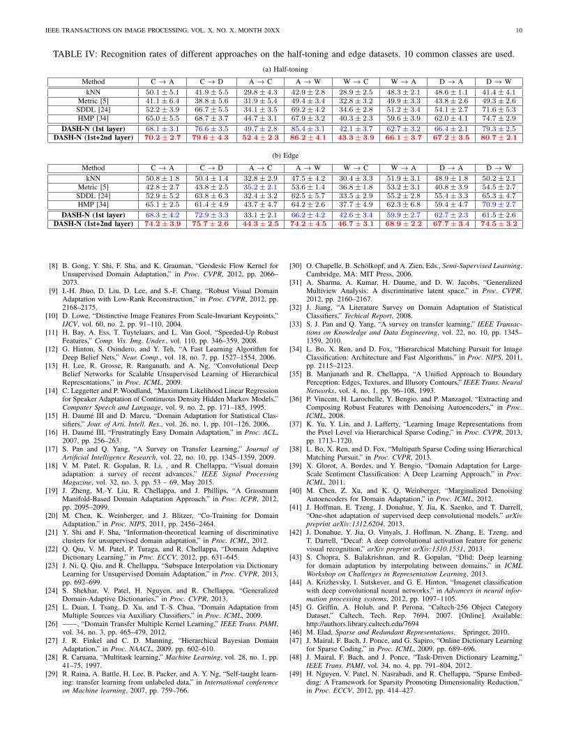
E. Halftoned and Edge ImagesIn order to evaluate the ability of DASH-N in adapting to

a wide range of domains, we also perform experiments onobject recognition from the original image domain to two newdomains generated by applying half-toning and edge extractionalgorithms to the original images. Half-toning images, whichimitate the effect of jet-printing technology in the past, aregenerated using the dithering algorithm in [53]. Edge imagesare obtained by applying the Canny edge detector [54] withthe threshold set to 0.07.

Figure 5 is the visualization of the reconstructed dictionariesatoms at layer 1 when adapting the original images (source) toedge images (target). Reconstructed dictionaries are obtainedby D1

∗ = (P1∗)†D1, where † denotes the MoorePenrose

pseudo-inverse. We observe that the dictionary atoms of orig-inal images contain rather fat and smooth regions. In contrast,dictionary atoms of edge images have many thin and highlyvarying patterns that are more suitable for capturing edges.Table IV shows the performance of different algorithms whenadapting to these new domains. It can be seen from thetable that DASH-N outperforms other methods used in thecomparison in both cases of half-toning and edge images.This proves the ability of our approach to adapt well to newdomains. As discussed in previous sections, although eventhe first layer of DASH-N already achieves very good resultson different settings, the performance consistently improveswith the addition of the second layer. In many cases, theimprovement in the recognition rates can be significant suchas in the case of C → A in Table I or A→W and D →Win Table IV which is more than 10%. Both the source codeand two new datasets will be released for research purposes.

F. Complexity Analysis

Let w and h be the width and height of an input image,respectively. Recall that d is the dimension of input sample.K(`) is the dictionary size at `-layer. q is the number of pixelsconsidered in the pooling operation. p(`) is the dimensionof the reduced space after the projection at `-layer. Thecomputation needed for evaluating an input image is givenas follows

O(w×h×d×p(1) + w×h×p(1)×K(1)×T (1)

+w×hq×K(1)×p(2) +

w×hq×p(2)×K(2)×T (2)

+w×hq2×K(2)×p(3) +

w×hq2×p(3)×K(3)×T (3))

= O(

3∑`=1

w×h×p(`)

q(`−1)(K(`−1) +K(`)×T (`))),

where we use the convention that K(0) is the equal to thedimension of the input patch d. We also assume that the sparsecoding for each sample could be performed with d×K×Tcomputation using OMP method or fast variants of Lasso.

VII. CONCLUSION

We have presented a hierarchical method for performingdomain adaptation using multi-layer representations of images.In the proposed approach, the features and domain shifts arelearned jointly in each layer of the hierarchy in order toobtain a better representation of data from different domains.Unlike other hierarchical approaches, our method prevents thedimension of feature vectors from increasing too fast as thenumber of layers increase. Experimental results show thatthe proposed approach significantly outperforms other domainadaptation algorithms considered in the comparison.

Several future directions of inquiry are possible consideringour new approach to domain adaptation and feature learning.It would also be of interest to incorporate non-linear learningframeworks to DASH-N.

ACKNOWLEDGMENT

This work was partially supported by a Grant from XEROX.

REFERENCES

[1] H. Shimodaira, “Improving predictive inference under covariate shift byweighting the log-likelihood function,” Journal of Statistical Planningand Inference, vol. 90, no. 2, pp. 227–244, 2000.

[2] N. Japkowicz and S. Stephen, “The class imbalance problem: A sys-tematic study,” Intelligent Data Analysis, vol. 6, no. 5, pp. 429–450,2002.

[3] S. Ben-David, J. Blitzer, K. Crammer, A. Kulesza, and F. Pereira,“A Theory of Learning from Different Domains,” Machine Learning,vol. 79, pp. 151–175, 2010.

[4] C. J. Stone, “Optimal Global Rates of Convergence for NonparametricRegression,” The Annals of Statistics, pp. 1040–1053, 1982.

[5] K. Saenko, B. Kulis, M. Fritz, and T. Darrell, “Adapting Visual CategoryModels to New Domains,” in Proc. ECCV, 2010, pp. 213–226.

[6] B. Kulis, K. Saenko, and T. Darrell, “What You Saw is Not What YouGet: Domain Adaptation using Asymmetric Kernel Transforms,” in Proc.CVPR, 2011, pp. 1785–1792.

[7] R. Gopalan, R. Li, and R. Chellappa, “Domain Adaptation for ObjectRecognition: An Unsupervised Approach,” in Proc. ICCV, 2011, pp.999–1006.


TABLE IV: Recognition rates of different approaches on the half-toning and edge datasets. 10 common classes are used.

(a) Half-toning

Method C → A C → D A → C A → W W → C W → A D → A D → WkNN 50.1± 5.1 41.9± 5.5 29.8± 4.3 42.9± 2.8 28.9± 2.5 48.3± 2.1 48.6± 1.1 41.4± 4.1

Metric [5] 41.1± 6.4 38.8± 5.6 31.9± 5.4 49.4± 3.4 32.8± 3.2 49.9± 3.3 43.8± 2.6 49.3± 2.6SDDL [24] 52.2± 3.9 66.7± 5.5 34.1± 3.5 69.2± 4.2 34.6± 2.8 51.2± 3.4 54.1± 2.7 71.6± 5.3HMP [34] 65.0± 5.5 68.7± 3.7 44.7± 3.1 67.9± 3.2 40.3± 2.3 59.6± 3.9 62.0± 4.1 74.7± 2.9

DASH-N (1st layer) 68.1± 3.1 76.6± 3.5 49.7± 2.8 85.4± 3.1 42.1± 3.7 62.7± 3.2 66.4± 2.1 79.3± 2.5DASH-N (1st+2nd layer) 70.2± 2.7 79.6± 4.3 52.4± 2.3 86.2± 4.1 43.3± 3.9 66.1± 3.7 67.2± 3.5 80.7± 2.1

(b) Edge

Method C → A C → D A → C A → W W → C W → A D → A D → WkNN 50.8± 1.8 50.4± 1.4 32.8± 2.9 47.5± 4.2 30.4± 3.3 51.9± 3.1 48.9± 1.8 50.2± 2.1

Metric [5] 42.8± 2.7 43.8± 2.5 35.2± 2.1 53.6± 1.4 36.8± 1.8 53.2± 3.1 40.8± 3.9 54.5± 2.7SDDL [24] 52.9± 5.2 63.8± 6.3 32.4± 3.2 62.5± 5.7 33.5± 2.9 55.2± 2.8 55.4± 3.3 65.3± 4.7HMP [34] 65.1± 2.5 61.4± 4.9 43.7± 4.7 64.2± 2.6 37.7± 4.9 62.3± 6.8 59.4± 4.7 70.9± 2.7

DASH-N (1st layer) 68.3± 4.2 72.9± 3.3 33.1± 2.1 66.2± 4.2 42.6± 3.4 59.9± 2.7 62.7± 2.3 61.5± 2.6DASH-N (1st+2nd layer) 74.2± 3.9 75.7± 2.6 44.3± 2.5 74.2± 4.5 46.7± 3.1 68.9± 2.2 67.7± 3.4 74.5± 3.2

[8] B. Gong, Y. Shi, F. Sha, and K. Grauman, “Geodesic Flow Kernel forUnsupervised Domain Adaptation,” in Proc. CVPR, 2012, pp. 2066–2073.

[9] I.-H. Jhuo, D. Liu, D. Lee, and S.-F. Chang, “Robust Visual DomainAdaptation with Low-Rank Reconstruction,” in Proc. CVPR, 2012, pp.2168–2175.

[10] D. Lowe, “Distinctive Image Features From Scale-Invariant Keypoints,”IJCV, vol. 60, no. 2, pp. 91–110, 2004.

[11] H. Bay, A. Ess, T. Tuytelaars, and L. Van Gool, “Speeded-Up RobustFeatures,” Comp. Vis. Img. Under., vol. 110, pp. 346–359, 2008.

[12] G. Hinton, S. Osindero, and Y. Teh, “A Fast Learning Algorithm forDeep Belief Nets,” Neur. Comp., vol. 18, no. 7, pp. 1527–1554, 2006.

[13] H. Lee, R. Grosse, R. Ranganath, and A. Ng, “Convolutional DeepBelief Networks for Scalable Unsupervised Learning of HierarchicalRepresentations,” in Proc. ICML, 2009.

[14] C. Leggetter and P. Woodland, “Maximum Likelihood Linear Regressionfor Speaker Adaptation of Continuous Density Hidden Markov Models,”Computer Speech and Language, vol. 9, no. 2, pp. 171–185, 1995.

[15] H. Daume III and D. Marcu, “Domain Adaptation for Statistical Clas-sifiers,” Jour. of Arti. Intell. Res., vol. 26, no. 1, pp. 101–126, 2006.

[16] H. Daume III, “Frustratingly Easy Domain Adaptation,” in Proc. ACL,2007, pp. 256–263.

[17] S. Pan and Q. Yang, “A Survey on Transfer Learning,” Journal ofArtificial Intelligence Research, vol. 22, no. 10, pp. 1345–1359, 2009.

[18] V. M. Patel, R. Gopalan, R. Li, , and R. Chellappa, “Visual domainadaptation: a survey of recent advances,” IEEE Signal ProcessingMagazine, vol. 32, no. 3, pp. 53 – 69, May 2015.

[19] J. Zheng, M.-Y. Liu, R. Chellappa, and J. Phillips, “A GrassmannManifold-Based Domain Adaptation Approach,” in Proc. ICPR, 2012,pp. 2095–2099.

[20] M. Chen, K. Weinberger, and J. Blitzer, “Co-Training for DomainAdaptation,” in Proc. NIPS, 2011, pp. 2456–2464.

[21] Y. Shi and F. Sha, “Information-theoretical learning of discriminativeclusters for unsupervised domain adaptation,” in Proc. ICML, 2012.

[22] Q. Qiu, V. M. Patel, P. Turaga, and R. Chellappa, “Domain AdaptiveDictionary Learning,” in Proc. ECCV, 2012, pp. 631–645.

[23] J. Ni, Q. Qiu, and R. Chellappa, “Subspace Interpolation via DictionaryLearning for Unsupervised Domain Adaptation,” in Proc. CVPR, 2013,pp. 692–699.

[24] S. Shekhar, V. Patel, H. Nguyen, and R. Chellappa, “GeneralizedDomain-Adaptive Dictionaries,” in Proc. CVPR, 2013.

[25] L. Duan, I. Tsang, D. Xu, and T.-S. Chua, “Domain Adaptation fromMultiple Sources via Auxiliary Classifiers,” in Proc. ICML, 2009.

[26] ——, “Domain Transfer Multiple Kernel Learning,” IEEE Trans. PAMI,vol. 34, no. 3, pp. 465–479, 2012.

[27] J. R. Finkel and C. D. Manning, “Hierarchical Bayesian DomainAdaptation,” in Proc. NAACL, 2009, pp. 602–610.

[28] R. Caruana, “Multitask learning,” Machine Learning, vol. 28, no. 1, pp.41–75, 1997.

[29] R. Raina, A. Battle, H. Lee, B. Packer, and A. Y. Ng, “Self-taught learn-ing: transfer learning from unlabeled data,” in International conferenceon Machine learning, 2007, pp. 759–766.

[30] O. Chapelle, B. Scholkopf, and A. Zien, Eds., Semi-Supervised Learning.Cambridge, MA: MIT Press, 2006.

[31] A. Sharma, A. Kumar, H. Daume, and D. W. Jacobs, “GeneralizedMultiview Analysis: A discriminative latent space,” in Proc. CVPR,2012, pp. 2160–2167.

[32] J. Jiang, “A Literature Survey on Domain Adaptation of StatisticalClassifiers,” Techical Report, 2008.

[33] S. J. Pan and Q. Yang, “A survey on transfer learning,” IEEE Transac-tions on Knowledge and Data Engineering, vol. 22, no. 10, pp. 1345–1359, 2010.

[34] L. Bo, X. Ren, and D. Fox, “Hierarchical Matching Pursuit for ImageClassification: Architecture and Fast Algorithms,” in Proc. NIPS, 2011,pp. 2115–2123.

[35] B. Manjunath and R. Chellappa, “A Unified Approach to BoundaryPerception: Edges, Textures, and Illusory Contours,” IEEE Trans. NeuralNetworks, vol. 4, no. 1, pp. 96–108, 1993.

[36] P. Vincent, H. Larochelle, Y. Bengio, and P. Manzagol, “Extracting andComposing Robust Features with Denoising Autoencoders,” in Proc.ICML, 2008.

[37] K. Yu, Y. Lin, and J. Lafferty, “Learning Image Representations fromthe Pixel Level via Hierarchical Sparse Coding,” in Proc. CVPR, 2013,pp. 1713–1720.

[38] L. Bo, X. Ren, and D. Fox, “Multipath Sparse Coding using HierarchicalMatching Pursuit,” in Proc. CVPR, 2013.

[39] X. Glorot, A. Bordes, and Y. Bengio, “Domain Adaptation for Large-Scale Sentiment Classification: A Deep Learning Approach,” in Proc.ICML, 2011.

[40] M. Chen, Z. Xu, and K. Q. Weinberger, “Marginalized DenoisingAutoencoders for Domain Adaptation,” in Proc. ICML, 2012.

[41] J. Hoffman, E. Tzeng, J. Donahue, Y. Jia, K. Saenko, and T. Darrell,“One-shot adaptation of supervised deep convolutional models,” arXivpreprint arXiv:1312.6204, 2013.

[42] J. Donahue, Y. Jia, O. Vinyals, J. Hoffman, N. Zhang, E. Tzeng, andT. Darrell, “Decaf: A deep convolutional activation feature for genericvisual recognition,” arXiv preprint arXiv:1310.1531, 2013.

[43] S. Chopra, S. Balakrishnan, and R. Gopalan, “Dlid: Deep learningfor domain adaptation by interpolating between domains,” in ICMLWorkshop on Challenges in Representation Learning, 2013.

[44] A. Krizhevsky, I. Sutskever, and G. E. Hinton, “Imagenet classificationwith deep convolutional neural networks,” in Advances in neural infor-mation processing systems, 2012, pp. 1097–1105.

[45] G. Griffin, A. Holub, and P. Perona, “Caltech-256 Object CategoryDataset,” Caltech, Tech. Rep. 7694, 2007. [Online]. Available:http://authors.library.caltech.edu/7694

[46] M. Elad, Sparse and Redundant Representations. Springer, 2010.[47] J. Mairal, F. Bach, J. Ponce, and G. Sapiro, “Online Dictionary Learning

for Sparse Coding,” in Proc. ICML, 2009, pp. 689–696.[48] J. Mairal, F. Bach, and J. Ponce, “Task-Driven Dictionary Learning,”

IEEE Trans. PAMI, vol. 34, no. 4, pp. 791–804, 2012.[49] H. Nguyen, V. Patel, N. Nasrabadi, and R. Chellappa, “Sparse Embed-

ding: A Framework for Sparsity Promoting Dimensionality Reduction,”in Proc. ECCV, 2012, pp. 414–427.


[50] V. M. Patel, H. V. Nguyen, and R. Vidal, “Latent space sparse subspaceclustering,” in International Conference on Computer Vision, 2013.

[51] Y.-L. Boureau, J. Ponce, and Y. LeCun, “A Theoretical Analysis ofFeature Pooling in Visual Recognition,” in Proc. ICML, 2010.

[52] Z. Wen and W. Yin, “A Feasible Method for Optimization with Orthog-onality Constraints,” Math. Prog., pp. 1–38, 2013.

[53] V. Monga, N. Damera-Venkata, H. Rehman, and B. Evans,“Halftoning MATLAB Toolbox,” http://users.ece.utexas.edu/ be-vans/projects/halftoning/toolbox/, 2005.

[54] J. Canny, “A Computational Approach to Edge Detection,” IEEE Trans.PAMI, vol. 8, no. 6, pp. 679–698, 1986.

[55] V. N. Vapnik, Statistical Learning Theory. John Wiley, 1998.[56] J. Yang, K. Yu, Y. Gong, and T. Huang, “Linear Spatial Pyramid

Matching using Sparse Coding for Image Classification,” in Proc. CVPR,2009, pp. 1794–1801.

[57] J. Yang, R. Yan, and A. Hauptmann, “Cross-Domain Video ConceptDetection using Adaptive SVMs,” in Proc. MM, 2007.

[58] M. Yang, L. Zhang, X. Feng, and D. Zhang, “Fisher DiscriminationDictionary Learning for Sparse Representation,” in Proc. CVPR, 2011,pp. 543–550.

[59] J. Deng, W. Dong, R. Socher, L.-J. Li, K. Li, and L. Fei-Fei, “Imagenet:A large-scale hierarchical image database,” in Computer Vision andPattern Recognition, 2009. CVPR 2009. IEEE Conference on. IEEE,2009, pp. 248–255.

[60] G. H. Golub and C. F. Van Loan, Matrix Computations, 4th ed. JohnsHopkins University Press, 2012.

APPENDIX

In this section, we provide the derivations for the forms ofD in (8) and Pi in (9) as well as extend the optimization tothe case of multiple source domains.

A. Form of D

We consider a general case where there are m differentdomains. Let {Yi,Pi,Xi, ni}mi=1 be the training data, thetransformation, the sparse coefficients, and the number ofsamples for the i-th domain, respectively. Let D denotethe common dictionary in the latent domain. The objectivefunction that we want to minimize is

m∑i=1

λiL(Yi,Pi,D,Xi, α, β)

=∑i

λi

(‖PiYi −DXi‖2F +α‖Yi −PT

i PiYi‖2F

+ β‖Xi‖1).

(23)

For the convenience of notation, we first define

Z = [√λ1P1Y1, . . . ,

√λmPmYm]. (24)

One can write D in the following form

D = D|| + D⊥, where D|| = ZB and DT⊥Z = 0, (25)

for some B ∈ R(∑

i ni)×K . In other words, columns of D||and D⊥ are in and orthogonal to the column subspace ofZ, respectively. Let S ∈ RK×K be a diagonal matrix withnon-negative coefficients such that columns of D|| = D||Shave unit-norm. Since the columns of D have unit-norm andD = D|| + D⊥, the columns of D|| must have norms of nolarger than 1. Therefore, in order for the columns of D|| tohave norm 1, the diagonal coefficients in S must be no lessthan 1. This gives us the following corollary

‖Xi‖1= ‖SS−1Xi‖1= ‖SXi‖1≥ ‖Xi‖1, (26)

where Xi = S−1Xi. In addition, we also have

‖PiYi −DXi‖2F = ‖PiYi −D||Xi‖2F +‖D⊥Xi‖2F≥ ‖PiYi −D||Xi‖2F= ‖PiYi − (D||S)(S−1Xi)‖2F= ‖PiYi − D||Xi‖2F . (27)

Using the two inequalities in (26) and (27), we can show thatm∑i=1


≥∑i

λi

(‖PiYi − D||Xi‖2F +α‖Yi −PT

i PiYi‖2F

+ β‖Xi‖1)

=

m∑i=1

λiL(Yi,Pi, D||, Xi, α, β).

(28)

This means that given any feasible solution (D,Xi), wecan find another feasible solution (D||, Xi), whose dictionaryatoms normalized to unit-norm, that does not increase the costfunction. Therefore, an optimal solution for D must be in formof D||, which can be generally written as

D = ZB = [√λ1P1Y1, . . . ,

√λmPmYm]B. (29)

B. Form of Pi

We perform the orthogonal decomposition of Pi as follows[60]

Pi = Pi⊥ + Pi||, where Pi⊥Yi = 0 and Pi|| = (YiAi)T .

(30)

In other words, rows of Pi|| and Pi⊥ are in and orthogonalto the column subspace of Yi, respectively. For convenienceof notation, let us define

P =

P1 . . . 0...

. . ....

0 . . . Pm

(31)

Y =

√λ1Y1

...√λmYm

(32)

X = (√λ1X1, . . . ,

√λmXm). (33)

After simple algebraic manipulations, the cost function can bere-written asm∑i=1


=∑i

λi

(‖PiYi− | DXi‖2F +α‖Yi −PT

i PiYi‖2F +β‖Xi‖1)

=(‖P||Y(I−BX)‖2F +αtr(YTY −P||YYTPT

|| )

+ β

m∑i=1

λi‖Xi‖1).

(34)


Removing all the terms independent of P, we have

tr(P||Y((I−BX)(I−BX)T − αI)YTPT

||

).

The objective function is independent of P⊥. Moreover, anoptimal solution of P|| is given by the eigenvectors of

Y((I−BX)(I−BX)T − αI)YT .

This means P||PT|| = I. However, P||P

T|| = I − P⊥PT

⊥,therefore, P⊥ = 0. We conclude that an optimal solution ofPi must have the following form

Pi = (YiAi)T , ∀i ∈ [1,m]. (35)

C. Optimization for Multiple Source Domains

The first term of (23) is∑i

λi‖PiYi −DXi‖2F = ‖Z(I−BX)‖2F , (36)

where X = [√λ1X1, . . . ,

√λmXm]. The second term of (23)

can be written as

α∑i

λi‖Yi −PTi PiYi‖2F = α

∑i

tr(Ki −YT

i PTi PiYi

)= α tr

(∑i

(Ki)− ZTZ).

(37)

After discarding all constant terms, the objective function in(23) is equivalent to

‖Z(I−BX)‖2F−α tr(ZTZ) + β∑i

λi‖Xi‖1. (38)

Solving for Ai: First, we perform the eigen-decompositionKi = ViΛiV

Ti . Then the eigen-decomposition of K is given

by

K = VΛVT , (39)

where,

V =

V1 . . . 0...

. . ....

0 . . . Vm

(40)

Λ =

√λ1Λ1 . . . 0

.... . .

...0 . . .

√λmΛm

. (41)

Moreover, let us define Gi = Λ12i VT

i Ai. Then, the constraintsbecome

PiPTi = AT

i KiAi = GTi Gi = I.

In order to solve for Ai, we assume that (B,Xi) are fixed.After removing all the terms independent of Ai, and using

(24) together with (39), the objective in (38) is equivalent to

‖Z(I−BX)‖2F−α tr(ZTZ)

= tr(Z((I−BX)(I−BX)T − αI)ZT

)= tr

(ATK((I−BX)(I−BX)T − αI)KA

)= tr

((ATVΛ

12 )(Λ

12 VT ((I−BX)(I−BX)T − αI)VΛ

12 )

(Λ12 VTA)

)= tr(GTHG),

(42)

where,

G = Λ12 VTA

=

V1 . . . 0...

. . ....

0 . . . Vm

√λ1Λ

T1 . . . 0

.... . .

...0 . . .

√λmΛT

m

A1

...Am

= [√λ1G1, . . . ,

√λmGm].

(43)

Then the solution of Ai can be obtained by first minimizing

minG

tr(GTHG) s.t. GTi Gi = I. (44)

This can be solved efficiently in the same way as for the caseof two domains using the algorithm proposed by [52]. Thesolution for Ai of each domain is recovered simply by

Ai = ViΛ− 1

2i Gi. (45)

Solving for (B,Xi): We now assume that Ai are fixed.After discarding the terms independent of (B,Xi) in (38),the objective function is re-written as

‖Z−DX‖2F +β∑i

λi‖Xi‖1. (46)

This is in the familiar form of dictionary learning problem. Weuse the online dictionary learning algorithm proposed by [47]to learn (D,Xi). The sparse coding is done using the LASSOalgorithm. After obtaining D, the solution of B is obtainedby

B = Z†D. (47)


PLACEPHOTOHERE

Hien V. Nguyen (M’08) is a research scientistat Siemens Corporate Technology in Princeton. Hereceived his bachelor and Ph.D. degrees in Electricaland Computer Engineering from the National Uni-versity of Singapore and the University of Marylandat College Park, respectively. His current researchinterests are in machine learning and pattern recog-nition algorithms for medical imaging and healthcareapplications.

PLACEPHOTOHERE

Huy Tho Ho (S’07) received the B.Eng. (withFirst-Class Hons.) degree in Computer SystemsEngineering, in 2007, and the M.App.Sc. degreein Electrical and Electronic Engineering, in 2009,both from the University of Adelaide, Australia. Hereceived the M.Sc. and Ph.D. degrees in Electri-cal and Computer Engineering from the Universityof Maryland (UMD), College Park, in 2013 and2014, respectively. His research interests includecomputer vision, machine learning and statisticalpattern recognition. Dr. Ho was a receiver of the

Adelaide Achiever Scholarship International (AASI) for his undergraduatestudy at the University of Adelaide, and the Clark School DistinguishedGraduate Fellowship at the University of Maryland, College Park.

PLACEPHOTOHERE

Vishal M. Patel (M’01) received the B.S. degreesin electrical engineering and applied mathematics(Hons.) and the M.S. degree in applied mathematicsfrom North Carolina State University, Raleigh, NC,USA, in 2004 and 2005, respectively, and the Ph.D.degree in electrical engineering from the Universityof Maryland College Park, MD, USA, in 2010. He iscurrently an Assistant Professor in the Department ofElectrical and Computer Engineering (ECE) at Rut-gers University. Prior to joining Rutgers University,he was a member of the research faculty with the

University of Marylands Institute for Advanced Computer Studies, CollegePark, MD, USA. His current research interests include signal processing,computer vision, and pattern recognition with applications in biometrics andimaging. He was a recipient of the ORAU Post-Doctoral Fellowship in 2010.He is a member of Eta Kappa Nu, Pi Mu Epsilon, and Phi Beta Kappa.

PLACEPHOTOHERE

Rama Chellappa (F’92) is a Minta Martin Pro-fessor of Engineering and Chair of the ECE depart-ment at the University of Maryland. Prof. Chellappareceived the K.S. Fu Prize from the InternationalAssociation of Pattern Recognition (IAPR). He isa recipient of the Society, Technical Achievementand Meritorious Service Awards from the IEEESignal Processing Society and four IBM faculty De-velopment Awards. He also received the TechnicalAchievement and Meritorious Service Awards fromthe IEEE Computer Society. At UMD, he received

college and university level recognitions for research, teaching, innovationand mentoring of undergraduate students. In 2010, he was recognized as anOutstanding ECE by Purdue University. Prof. Chellappa served as the Editor-in-Chief of PAMI. He is a Golden Core Member of the IEEE ComputerSociety, served as a Distinguished Lecturer of the IEEE Signal ProcessingSociety and as the President of IEEE Biometrics Council. He is a Fellow ofIEEE, IAPR, OSA, AAAS, ACM and AAAI and holds four patents

Date post:	24-Mar-2018
Category:	Documents
Upload:	buiduong
View:	222 times
Download:	1 times

IEEE TRANSACTIONS ON IMAGE PROCESSING, …vmp93/Journal_pub/DASHN_TIP_revised_final.pdfIEEE...

Documents