IEEE TRANSACTIONS ON IMAGE PROCESSING, VOL. … · optimization problem is solved by transforming...

IEEE TRANSACTIONS ON IMAGE PROCESSING, VOL. 20, NO. 11, NOVEMBER 2011 3097

An Augmented Lagrangian Method for TotalVariation Video Restoration

Stanley H. Chan, Student Member, IEEE, Ramsin Khoshabeh, Student Member, IEEE,Kristofor B. Gibson, Student Member, IEEE, Philip E. Gill, and Truong Q. Nguyen, Fellow, IEEE

Abstract—This paper presents a fast algorithm for restoringvideo sequences. The proposed algorithm, as opposed to existingmethods, does not consider video restoration as a sequence ofimage restoration problems. Rather, it treats a video sequenceas a space–time volume and poses a space–time total variationregularization to enhance the smoothness of the solution. Theoptimization problem is solved by transforming the original un-constrained minimization problem to an equivalent constrainedminimization problem. An augmented Lagrangian method is usedto handle the constraints, and an alternating direction methodis used to iteratively find solutions to the subproblems. The pro-posed algorithm has a wide range of applications, including videodeblurring and denoising, video disparity refinement, and hot-airturbulence effect reduction.

Index Terms—Alternating direction method (ADM), augmentedLagrangian, hot-air turbulence, total variation (TV), video deblur-ring, video disparity, video restoration.

I. INTRODUCTION

A. Video Restoration Problems

I MAGE RESTORATION is an inverse problem where theobjective is to recover a sharp image from a blurry and noisy

observation. Mathematically, a linear shift invariant imagingsystem is modeled as [1]

(1)

where is a vector denoting the unknown (poten-tially sharp) image of size , is a vectordenoting the observed image, is a vector denotingthe noise, and matrix is a linear transformationrepresenting convolution operation. The goal of image restora-tion is to recover from .

Manuscript received October 29, 2010; revised February 24, 2011 and April26, 2011; acceptedMay 05, 2011. Date of publicationMay 31, 2011; date of cur-rent version October 19, 2011. The work of S. Chan was supported by CroucherFoundation Scholarship, Hong Kong. The work of R. Khoshabeh was supportedby the University of California, San Diego, under Program CalIT2 CSRO. Thework of K. Gibson was support by the Space and Naval Warfare Systems CenterPacific (SSC Pacific) Naval Innovative Science and Engineering Program. TheAssociate Editor coordinating the review of this manuscript and approving it forpublication was Prof. Sina Farsiu.S. H. Chan, R. Khoshabeh, K. B. Gibson, and T. Q. Nguyen are with the

Department of Electrical and Computer Engineering, University of California,San Diego, La Jolla, CA 92093-0112 USA (e-mail: [email protected]).P. E. Gill is with the Department of Mathematics, University of California,

San Diego, La Jolla, CA 92093-0112 USA.Color versions of one or more of the figures in this paper are available online

at http://ieeexplore.ieee.org.Digital Object Identifier 10.1109/TIP.2011.2158229

Standard single-image restoration has been studied for morethan half a century. Popular methods such as Wiener deconvo-lution [1], Lucy Richardson deconvolution [2], [3], and regular-ized least squares minimization [4], [5] have already been im-plemented in MATLAB and FIJI [6]. Advanced methods suchas variational methods are also becoming mature [7]–[11].While single-image restorations still have a room for im-

provement, we consider in this paper the video restorationproblem. The key difference between an image and a video isthe additional time dimension. Consequently, video restora-tion has some unique features that do not exist in an imagerestoration.1) Motion informationMotion deblurring requires motion vector field, which canbe estimated from a video sequence using conventionalmethods such as block matching [12] and optical flow [13].While it is also possible to remove motion blur based on asingle image, for example, [14]–[18], the performance islimited to a global motion or, at most, one to two objectsby using sophisticated object segmentation algorithms.

2) Spatial variance versus spatial invarianceFor a class of spatially variant image restoration problems(in particular motion blur), the convolution matrix isnot a block-circulant matrix. Therefore, Fourier transformscannot be utilized to efficiently find a solution. Videos,in contrast, allow us to transform a sequence of spatiallyvariant problems to a spatially invariant problem (See thenext section for more discussions). As a result, a huge gainin speed can be realized.

3) Temporal consistencyTemporal consistency is concerned about the smooth-ness of the restored video along the time axis. Althoughsmoothing can be spatially performed (as in the case ofsingle image restoration), temporal consistency cannot beguaranteed if these methods are applied to a video in aframe-by-frame basis.

Because of these unique features of a video, we seek a videorestoration algorithm that utilizes motion information, exploitsthe spatially invariant properties, and enforces spatial and tem-poral consistency.

B. Related Work

There are many works on the problem of video restora-tion, particularly in the domain of video superresolution. In[19]–[21], video superresolution is formulated in a regularizedleast square minimization framework, in which the bilateraltotal variation (TV) is used as the regularization function.Later, in [22] and [23], the concept of kernel regression to the

1057-7149/$26.00 © 2011 IEEE

3098 IEEE TRANSACTIONS ON IMAGE PROCESSING, VOL. 20, NO. 11, NOVEMBER 2011

video restoration problem is applied. Similar approaches canbe also found in [24], where Ng et al. considered isotropic TVas the a regularization function and modified (1) to incorporatethe geometric warp caused by motion. In [25], Belekos et al.proposed a novel prior that utilizes the motion vector field inupdating the regularization parameters so that the prior is bothspatially and temporally adaptive to the data. A recent work byChan and Nguyen [26] has considered a regularization functionof the residue between the current solution and the motioncompensated version of the previous solution.It is worth noting that most of the aforementioned methods

recover a video in a frame-by-frame basis.1 Additionally, all ofthese methods assume that the blur kernel is spatially invariant.While this assumption is valid for many superresolution sce-narios where multiple shots of the same object are used to fusea higher resolution image, it is invalid when the blur is causedby object motions. As a result, they are unable to handle the spa-tially variant motion blur kernel.Our proposed algorithm is inspired by the concept of

“space–time volume,” which is first introduced in the early 90sby Jähne [27], and rediscovered by Wexler, Shechtman, Caspi,and Irani [28], [29]. The idea of space–time volume is to stackthe frames of a video to form a 3-D data structure known as thespace–time volume. This allows one to transform the spatiallyvariant motion blur problem to a spatially invariant problem.By imposing regularization functions along the spatial andtemporal directions, respectively, both spatial and temporalsmoothness can be enforced.The main drawback of space–time minimization is that the

size of a space–time volume is much larger than that of a singleimage (or five frames in the case of [25]). Therefore, the authorsof [29] only considered a Tikhonov regularized least squareminimization ([29, eq. (3)]) in which a closed-form solutionexists. More sophisticated regularization functions such as TVand bilateral TV do not seem possible under this frameworkfor these nondifferentiable functions are difficult to efficientlysolve.This paper investigates the TV regularization functions

in space–time minimization. In particular, we consider thefollowing two problems:

minimize (2)

which is known as the TV/L2 minimization and

minimize (3)

which is known as the TV/L1 minimization. Unless specified,norms and are the conventional vector 2-norm squaresand the vector 1-norm, respectively. TV-norm can eitherbe the anisotropic TV norm

(4)

1A version of [25] is able to simultaneously process multiple frames, but inpractice, it only supports five frames at once.

or the isotropic TV norm

(5)

where operators , , and are the forward finite-differ-ence operators along the horizontal, vertical, and temporal di-rections, respectively. Here, are constants, anddenotes the th component of the vector . More details on thesetwo equations will be discussed in Section II-C.The proposed algorithm is based on the augmented La-

grangian method, which is an old method that has recentlydrawn significant attention [10], [11], [30]. Most of the existingaugmented Lagrangian methods for image restoration followfrom Eckstein and Bertsekas’ operator splitting method [31],which can be traced back to the work of Douglas and Rachford[32], and the proximal point algorithm by Rockafellar [33],[34]. Recently, the operator splitting method has been provento be equivalent to the splitting Bregman iteration for someproblems [35], [36]. However, there is no work on extendingthe augmented Lagrangian method to space–time minimization.

C. Contributions

The contribution of this paper is summarized as follows.1) We extend the existing augmented Lagrangian method tosolve space–time TV minimization problems (2) and (3).Augmented Lagrangian method was previously used toimage restoration only [10], [11].

2) Half-quadratic penalty parameter is updated according toconstraint violation. This leads to faster rate of conver-gence, compared with methods using a fixed parameter[10].

3) Because of the space–time data structure, our proposedalgorithm is able to handle spatially variant motion blurproblems (object motion blur). Existing methods such as[19]–[26] are unable to do so.

4) Compared with [29], which is also a space–time minimiza-tion method, our method achieves TV/L1 and TV/L2 min-imization quality, whereas [29] only achieves Tikhonovleast square minimization quality.

5) In terms of speed, we achieve significantly faster compu-tational speed, compared with existing methods. Typicalrun time to deblur and denoise a 300 400 gray-scaledvideo is a few second per frame on a personal computer(PC) (MATLAB). This implies the possibility of real-timeprocessing on a graphics-processing unit.

6) The proposed algorithm supports a wide range ofapplications.a) Video deblurring: With the assistance of frame rateup-conversion algorithms, the proposed method canremove spatially variant motion blur for real videosequences;

b) Video disparity: Occlusion errors and temporal incon-sistent estimates in the video disparity can be handledby the proposed algorithm without any modification;

c) Hot-air turbulence: The algorithm can be directlyused to deblur and remove hot-air turbulence effects.

CHAN et al.: AUGMENTED LAGRANGIAN METHOD FOR TOTAL VARIATION VIDEO RESTORATION 3099

D. Organization

This paper is an extension of two recently accepted confer-ence papers [37], [38]. The organization of this paper is as fol-lows: Section II consists of notations and background materials.The algorithms are discussed in Section III. Section IV dis-cusses three applications of the proposed algorithm, namely, 1)video deblurring, 2) video disparity refinement, and 3) hot-airturbulence effects reduction. A concluding remark is given inSection V.

II. BACKGROUND AND NOTATION

A. Notation

A video signal is represented by a 3-D function ,where denotes the coordinate in space and denotes thecoordinate in time. Suppose that each frame of the video hasrows, columns, and there are frames, then, the discrete

samples of for , ,and form a 3-D tensor of size .For the purpose of discussing numerical algorithms, we

use matrices and vectors. To this end, we stack the entries ofinto a column vector of size , according

to the lexicographic order. We use the bold letter to representthe vectorized version of the space–time volume , i.e.,

where represents the vectorization operator.

B. Three-Dimensional Convolution

The 3-D convolution is a natural extension of the conven-tional 2-D convolution. Given space–time volume andthe blur kernel , the convolved signal is given

by. Convolution is a linear operation; therefore, it

can be expressed using matrices. More precisely, we define theconvolution matrix associated with a blur kernel asthe linear operator that maps signal to fol-lowing the rule, i.e.,

(6)

Assuming periodic boundaries [39], the convolution matrixis a triple block-circulant matrix—it has a block-circulant struc-ture, and within each block, there is a submatrix of block circu-lant with circulant block. Circulant matrices are diagonalizableusing discrete Fourier transform (DFT) matrices [40], [41]:

Fact 1: If is a triple block-circulant matrix, then it canbe diagonalized by the 3-D DFT matrix as

where is the Hermitian operator and is a diagonalmatrix storing the eigenvalues of .

C. Forward-Difference Operators

We define operator as a collection of three suboperators, where , , and are the first-

order forward finite-difference operators along the horizontal,vertical, and temporal directions, respectively. The definitionsof each individual suboperators are

with periodic boundary conditions.In order to have greater flexibility in controlling the forward

difference along each direction, we introduce three scalingfactors as follows. We define scalars , , and andmultiply them with , , and , respectively, so that

.With , the anisotropic TV norm and the

isotropic TV are defined according to (4) and (5), re-spectively. When and , is the 2-DTV of (in space). When and ,is the 1-D TV of (in time). By adjusting , , and , wecan control the relative emphasis put on individual terms ,

, and .Note that is equivalent to the vector 1-norm on ,

i.e., . Therefore, for notation simplicity, weuse instead. For , although

using the vector 2-norm definition, we still defineto align with the definition of . However, this

will be made clear if confusion arises.

III. PROPOSED ALGORITHM

The proposed algorithm belongs to the family of operatorsplitting methods [10], [11], [31]. Therefore, instead of re-peating the details, we focus on the modifications made to the3-D data structure. Additionally, our discussion is focused onthe anisotropic TV, i.e., . The isotropic TV, canbe similarly derived.

A. TV/L2 Problem

The core optimization problem that we solve is the followingTV/L2 minimization:

minimize (7)

where is a regularization parameter. To solve problem (7), wefirst introduce intermediate variables and transform problem(7) into an equivalent problem, i.e.,

minimize

subject to (8)


The augmented Lagrangian of problem (8) is

(9)

where is a regularization parameter associated with thequadratic penalty term and is the Lagrangemultiplier associated with the constraint . In (9),intermediate variable and Lagrange multiplier can berespectively partitioned as

and(10)

The idea of the augmented Lagrangian method is to find asaddle point of , which is also the solution of the orig-inal problem (7). To this end, we use the alternating directionmethod to iteratively solve the following subproblems:

(11)

(12)

(13)

We now investigate these subproblems one by one.1) -Subproblem: By dropping indexes , the solution of

problem (11) is found by considering the normal equation asfollows:

(14)

The convolution matrix in (14) is a triple block-circulantmatrix, and therefore, by Fact 1, can be diagonalized usingthe 3-D DFT matrix. Hence, (14) has the following solution:

(15)

where denotes the 3-D Fourier transform operator. The ma-trices , , , and can be precalculatedoutside the main loop. Therefore, the complexity of solving (14)is in the order of operations, which is the complexityof the 3-D Fourier transforms, and is the number of elementsof the space–time volume .2) -Subproblem: Problem (12) is known as the -sub-

problem, which can be solved using a shrinkage formula [42].Letting (analogous definitions forand ), is given by

sign (16)

Analogous solutions for and can be also derived.

In case of isotropic TV, the solution is given by [42]

(17)

where , and is a smallconstant . Here, the multiplication and divisions arecomponentwise operations.3) Algorithm: Algorithm 1 shows the pseudocode of the

TV/L2 algorithm.

Algorithm 1 Algorithm for TV/L2 minimization problem

Input data and .

Input parameters , , , and .

Set parameters default and default .

Initialize , , , .

Compute the matrices , , , and .

while not converge do

1. Solve the -subproblem (11) using (15).

2. Solve the -subproblem (12) using (16).

3. Update the Lagrange multiplier using (13).

4. Update according to (24).

5. Check convergence:

if then

break

end if

end while

B. TV/L1 Problem

TV/L1 problem can be solved by introducing two interme-diate variables, i.e., and , and modifying problem (3) as

minimize

subject to

(18)

The augmented Lagrangian of (18) is given by

.Here, variable is the Lagrange multiplier associated withconstraint , and variable is the Lagrange multiplierassociated with the constraint . Moreover, andcan be partitioned as in (10). Parameters and are two

regularization parameters. Subscripts “ ” and “ ” stand for“objective” and “regularization,” respectively.


Fig. 1. TV/L2 image recovery using different choices . The optimal (in terms of PSNR compared to the reference) is . The image is blurred by aGaussian blur kernel of size 9 9 and . Addition Gaussian noise is added to the image so that the BSNR is 40 dB.

1) -Subproblem: The -subproblem of TV/L1 is

minimize

(19)

which can be solved by considering the following normalequation:

yielding

(20)

2) -Subproblem: The -subproblem of TV/L1 is the sameas that of TV/L2. Therefore, the solution is given by (16).3) -Subproblem: The -subproblem is

minimize (21)

Thus, using the shrinkage formula, the solution is

sign

(22)

4) Multiplier Update: and are updated as

(23)

5) Algorithm: Algorithm 2 shows the pseudocode of theTV/L1 algorithm.

Algorithm 2 Algorithm for TV/L1 minimization problem

Input , , and parameters , , , and . Let .Set parameters default , default , and

default .Initialize , , , , and

.Compute matrices , , , and .while not converge do

1. Solve the -subproblem (19) using (20).2. Solve the -subproblem (12) using (16).3. Solve the -subproblem (21) using (22).4. Update and using (23).5. Update and according to (24).6. Check convergence:

if tol then

break

end if

end while

C. Parameters

In this subsection, we discuss the choice of parameters.1) Choosing : The regularization parameter trades off the

least square error and the TV penalty. Large values of tend togive sharper results, but noise will be amplified. Small valuesof give less noisy results, but the image may be smoothed.The choice of is not known prior to solving the minimization.Recent advances in the operator-splitting methods have consid-ered constrained minimization problems [11] so that can bereplaced by an estimate of the noise level (the noise estimationis performed using a third party algorithm). However, from ourexperience, it is often easier to choose than to estimate thenoise level for the noise characteristic of a video is never exactlyknown. Empirically, a reasonable for a natural image (andvideo sequence) typically lies in the range . Figs. 1and 2 show the recovery results by using different values of .In the case of TV/L1 minimization, is typically lying in therange [0.1, 10].


Fig. 2. TV/L1 image recovery using different choices . The optimal (in terms of PSNR compared to the reference) is . The image is blurred by a Gaussianblur kernel of size 9 9 and of the pixels are corrupted by salt and pepper noise. Image source: [43].

2) Choosing : One of the major differences between theproposed algorithm and FTVd 4.0 [35]2 is the update of . In[35], is a fixed constant. However, as mentioned in [44], themethod of multipliers can exhibit a faster rate of convergenceby adapting the following parameter update scheme:

ifotherwise.

(24)

Here, condition spec-ifies the constraint violation with respect to constant . Theintuition is that the quadratic penalty is aconvex surface added to the original objective function

so that the problem is guaranteed to be stronglyconvex [33]. Ideally, residue should de-crease as increases. However, if is notdecreasing for some reasons, one can increase the weight ofpenalty , relative to the objective, so that

is forced to be reduced. Therefore, givenand , where and , (24) makes sure that theconstraint violation is asymptotically decreasing. In the steadystate, as , becomes a constant [46]. The update forin TV/L1 follows a similar approach.The initial value of is chosen to be within the range of [2,

10]. This value cannot be large (in the order of 100) becausethe role of the quadratic surface is to perturb theoriginal objective function so that it becomes strongly convex.If the initial value of is too large, the solution of the originalproblem may not be found. However, cannot be too smalleither; otherwise, the effect of the quadratic surfacebecomes negligible. Empirically, we find that is robustto most restoration problems.

D. Convergence

Fig. 3 illustrates the convergence profile of the TV/L2 algo-rithm in a typical image recovery problem. In this test, the image“cameraman.tif” (size 256 256; gray scaled) is blurred by aGaussian blur kernel of size 9 9 and . Gaussian noise isadded so that the blurred signal-to-noise ratio (BSNR) is 40 dB.To visualize the effects of the parameter update scheme, we setthe initial value of to be , and let . Referringto (24), is increased by a factor of if the condition is sat-

2The most significant difference is that FTVd 4.0 supports only images,whereas the proposed algorithm supports videos.

Fig. 3. Convergence profile of the proposed algorithm for deblurring the image“cameraman.tif”. (Four colored curves) The rate of convergence using differentvalues of , where is the multiplication factor for updating .

isfied. Note that [35] (FTVd 4.0) is a special case when ,whereas the proposed algorithm allows the user to vary .In Fig. 3, the -axis is the objective value

for the th iteration, and the -axis is iteration number. As shown in the figure, an appropriate choice of signifi-cantly improves the rate of convergence. However, if is toolarge, the algorithm is not converging to the solution. Empiri-cally, we find that is robust to most of the image andvideo problems.

E. Sensitivity Analysis

Table I illustrates the sensitivity of the algorithm to parame-ters , , and . In this test, 20 images are blurred by aGaussianblur kernel of size 9 9, with variance . The BSNRis 30 dB. For each image, two of the three parameters ( , ,and ) are fixed at their default values, i.e., , ,and , whereas one of them is varying within the rangespecified in Table I. The stopping criteria of the algorithm is

, , andfor all images. The maximum peak signal-to-noise ratio

(PSNR), minimum PSNR, and the difference are reported inTable I. Referring to the values, it can be calculated that the av-erage maximum-to-minimum PSNR differences among all 20images for , , and are 0.311, 0.208, and 0.357 dB, respec-tively. For an average PSNR difference in the order of 0.3 dB,the perceivable difference is small.3

3It should be noted that the optimization problem is identical for all parametersettings. Therefore, the correlation between the PSNR and visual quality is high.


TABLE ISENSITIVITY ANALYSIS OF PARAMETERS. MAXIMUM AND MINIMUM PSNR (IN DECIBELS) FOR A RANGE OF , , AND .

IF A PARAMETER IS NOT THE VARIABLE, IT IS FIXED AT DEFAULT VALUES , , AND

F. Comparison With Existing Operator-Splitting Methods

The proposed algorithm belongs to the class of operator split-ting methods. Table II summarizes the differences between theproposed method and some existing methods.4

IV. APPLICATIONS

In this section, we demonstrate three applications of theproposed algorithm, namely, 1) video deblurring, 2) video dis-parity refinement, and 3) video restoration for videos distortedby hot-air turbulence. Due to limited space, more results areavailable at http://videoprocessing.ucsd.edu/stanleychan/de-convtv.

A. Video Deblurring

1) Spatially Invariant Blur: We first consider the class ofspatially invariant blur. In this problem, the th observed image

is related to the true image as

Note that the spatially invariant blur kernel is assumedto be identical for all time .The typical method to solve a spatially invariant blur is to

consider the model as

4The speed comparison is based on deblurring “lena.bmp” (512 512; grayscaled), which is blurred by a Gaussian blur kernel of size 9 9, , andBSNR dB. The machine used is Intel Qual Core at 2.8 GHz, with 4-GBrandom access memory (RAM), and Windows 7/MATLAB 2010. Comparisonsbetween FTVd 4.0 and the proposed method are based on . If(default setting of FTVd 4.0), then the run time are 1.56 and 1.28 s for FTVd4.0 and the proposed method, respectively.

and apply a frame-by-frame approach to individually recover. In [26], the authors considered the following minimization:

minimize

where is the solution of the th frame and is themotion compensation operator that maps the coordinates ofto the coordinates of . Operators are the spatial forwardfinite-difference operators oriented at angles 0 , 45 , 90 , and135 . Regularization parameters and control the relativeemphasis put on the spatial and temporal smoothness.Another method to solve the spatially invariant blur problem

is to apply the multichannel approach by modeling the imagingprocess as [24], [25]

for , where is the size of thetemporal window (typically ranged from 1 to 3). is themotion compensation operator that maps the coordinates ofto the coordinates of . The th frame can be recovered bysolving the following minimization [24]:

minimize (25)

where is a constant and is the isotropic TV on the thframe. Themethod presented in [25] replaces the objective func-tion by a weighted least squares and the isotropic TV regular-ization function by a weighted 2-norm on gradient. The weightsare adaptively updated (using residue and motion vector field)in each iteration, and therefore, the regularization function isnonstationary, both spatially and temporally.


TABLE IICOMPARISONS BETWEEN THE OPERATOR-SPLITTING METHODS FOR TV/L2 MINIMIZATION

TABLE IIICOMPARISONS BETWEEN THE VIDEO RESTORATION METHODS

A drawback of these methods is that the image recovery re-sult heavily depends on the accuracy of motion estimation andcompensation. In particular, in occlusion areas, the assumptionthat is a one-to-one mapping [47] fails to hold. Thus,is not a full-rank matrix, and . As a result, mini-mizing can lead to a serious error. There aremethods to reduce the error caused by rank deficiency of ,for example, the concept of unobservable pixel introduced in[24], but the restoration result depends on the effectiveness ofhow the unobservable pixels are selected.Another drawback of these methods is the computation time.

For spatially invariant blur, blur operator is a block-circulantmatrix. However, in the multichannel model, the operator

is not a block-circulant matrix. The block-circulantproperty is a critical factor to speed as it allows the use ofFourier transform methods. For methods in [24] and [25],conjugate gradient (CG) is used to solve the minimizationtask. While the total number of CG iterations may be few, theper-iteration run time can be long.Table III illustrates the differences between various video

restoration methods.Our approach to solve spatially invariant blur problem shares

the same insight as [29], which does not consider motion com-pensation. The temporal error is handled by spatio–temporalTV . An in-tuition to this approach is that the temporal differencecan be classified as temporal edge and temporal noise. The tem-poral edge is the intensity change caused by object movements,whereas the temporal noise is the artifact generated in the min-imization process. Similar to the spatial TV, the temporal TVpreserves the temporal edges while reducing the temporal noise.Moreover, the space–time volume preserves the block-circu-

TABLE IVPSNR, , AND VALUES FOR FOUR VIDEO SEQUENCES BLURRED BY

GAUSSIAN BLUR KERNEL 9 9, , AND BSNR dB

lant structure of the operator, thus leading to significantly fastercomputation.Table IV, and Figs. 4 and 5 show the comparisons between

[24], [26], and [29] and the proposed method on spatially in-variant blur. The four testing video sequences are blurred bya Gaussian blur kernel of size 9 9 with . AdditiveGaussian noise are added so that the BSNR is 30 dB.The specific settings of the methods are as follows. For [29],

we consider the following minimization:

minimize

and set the parameters empirically for the best recovery quality:and . For [24], instead of


Fig. 4. “News” sequence; frame 100. (a) Original image (cropped for bettervisualization). (b) Blurred by a Gaussian blur kernel of size 9 9, , andBSNR dB. (c)–(f) Results by various methods (see Table IV).

using the CG presented in this paper, we use a modificationof the proposed augmented Lagrangian method to speed up thecomputation. Specifically, in solving the -subproblem, we usedCG (LSQR [48]) to accommodate the nonblock-circulant op-erator . The motion estimation is performed using thebenchmark full search (exhaustive search) with 0.5-pixel accu-racy. The block size is 8 8, and the search range is 1616. Motion compensation is performed by coordinate transformaccording to the motion vectors (bilinear interpolation for halfpixels). The threshold for unobservable pixels [24] is set as 6(out of 255), and the regularization parameter is [see(25)]. We use the previous and the next frame for the model, i.e.,

and let (Using (1, 1, 1)tends to give worse results). For [26], the regularization param-eters are also empirically chosen for the best recovery quality:

and .To compare these methods, we apply TV/L2 (Algorithm 1)

with the following parameters (same for all four videos):and . All other parameters take the

default setting: , , and . The algorithmterminates if .

Fig. 5. “Salesman” sequence; frame 10. (a) Original image (cropped for bettervisualization). (b) Blurred by a Gaussian blur kernel of size 9 9, , andBSNR dB. (c)–(f) Results by various methods (see Table IV).

In Table IV, three quantities are used to evaluate the perfor-mance of the algorithms. PSNR measures the image fidelity.Spatial TV is defined asfor each frame, and temporal TV is defined as

for each frame [26]. The average (overall frames) PSNR, , and are listed in Table IV.Referring to the results, it is shown that the proposed al-

gorithm produces the highest PSNR values while keepingand at a low level. It is worth noting that [29] is equiva-lent to the 3-D Wiener deconvolution (regularized). Therefore,there exists a closed-form solution, but the result looks blurrierthan the other methods. Among the four methods, both [24] and[26] use motion estimation and compensation. However, [24]is more sensitive to the motion estimation error—motion esti-mation error in some fast-moving areas are amplified in the de-blurring step. Reference [26] is more robust to motion estima-tion error, but the computation time is significantly longer thanthe proposed method. The run time of [24] and [26] are approx-imately 100 s per frame (per color channel), whereas the pro-posed algorithm only requires approximately 2 s per frame (percolor channel). These statistics are based on recovering videosof size 288 352, using a PC with Intel Qual Core at 2.8 GHz,with 4-GB RAM, and Windows 7/MATLAB 2010.


Fig. 6. “Market Place” sequence; frame 146. (Top) The original observed videosequences. (Middle) Result of [29]. (Bottom) Result of the proposed method.

2) Spatially Variant Motion Blur: The proposed algorithmcan be used to remove spatially variant motion blur. However,sincemotion-blurred videos often have low temporal resolution,frame rate up-conversion algorithms are needed to first increasethe temporal resolution before applying the proposed method(see [29] for detailed explanations). To this end, we apply [49]to upsample the video by a factor of 8. Consequently, the motionblur kernel can be modeled as

if , andotherwise

where in this case.Fig. 6 shows frame no. 146 of the video sequence “Market

Place,” and Fig. 7 shows frame no. 28 of the video sequence“Super Loop.” The videos are captured by a Panasonic TM-700video recorder with resolution 1920 1080p at 60 fps. For com-putational speed, we down sampled the spatial resolution by afactor of 4 (so the resolution is 480 270). The parameters ofthe proposed algorithm are empirically chosen as and

. There are not many relevant video mo-tion deblurring algorithms for comparison (or unavailable to betested). Therefore, we are only able to show the results of [29],using parameters and .As shown in Figs. 6 and 7, the proposed algorithm produces a

significantly higher quality result than [29]. We also tested for arange of parameters and for [29]. However, we observe thatthe results are either oversharpened (serious ringing artifacts) orundersharpened (not enough deblurring).3) Limitation: The proposed algorithm requires considerably

less memory than other TV minimization algorithms such asinterior point methods. However, for high-definition videos, theproposed algorithm still has a memory issue as the size of thespace–time volume is large. While one can use fewer frames

Fig. 7. “Super Loop” sequence; frame 28. (Top) The original observed videosequences. (Middle) Result of [29]. (Bottom) Result of the proposed method.

Fig. 8. (Top) Before applying the proposed TV/L1 algorithm. (Middle) Afterapplying the proposed TV/L1 algorithm. (Bottom) Time evolution of the dis-parity value (normalized) of a pixel.

to lower the memory demand, trade off in the recovery qualityshould be expected.Another bottleneck of the proposed algorithm is the sensi-

tivity to the frame-rate conversion algorithm. At object bound-aries where the motion estimation algorithm fails to provide ac-curate estimates, the estimation error in the deblurring step willbe amplified. This typically happens to areas with nonuniformand rapid motion.


Fig. 9. Video disparity estimation. (First row) Left view of the stereo video. (Second row) Initial disparity estimate. (Third row) Refinement using the proposedmethod with parameters , , , , , and . (Last row) Zoom-in comparisons. (a) “Old Timers”sequence. (b) “Horse” sequence.

B. Video Disparity Refinement

1) Problem Description: Our second example is disparitymap refinement. Disparity is proportional to the reciprocal ofthe distance between the camera and the object (i.e., depth).Disparity maps are useful for many stereo-video processing ap-plications, including object detection in 3-D space, saliency forstereo videos, stereo coding, and view synthesisThere are numerous papers on generating one disparity map

based on a pair of stereo images [50]. However, all of thesemethods cannot be extended to videos because the energyfunctions are considered in a frame-by-frame basis. Althoughthere are works in enforcing temporal consistency for adjacentframes, such as [51] and [52], the computational complexity ishigh.We propose to estimate the video disparity in two steps. In the

first step, we combine the locally adaptive support weight [53]and the cross-bilateralateral grid [54] to generate an initial dis-parity estimate. Since this method is a frame-by-frame method,spatial and temporal consistency is poor. In the second step, weconsider the initial video disparity as a space–time volume andsolve the TV/L1 minimization problem, i.e.,

minimize

There are two reasons for choosing TV/L1 instead of TV/L2in refining video disparity. First, disparity is a piecewise con-stant function with quantized levels, and across the flat regions,there are sharp edges. As shown in Fig. 8 (bottom), the estima-tion error behaves like outliers in a smooth function. Therefore,to reduce the estimation error, one can consider a robust curvefitting as it preserves the shape of the data while suppressing theoutliers.The second reason for using TV/L1 is that the 1-normis related to the notion of percentage of bad pixels, which is

a quantity commonly used to evaluate disparity estimation al-gorithms [50]. Given a ground truth disparity , the numberof bad pixels of an estimated disparity is the cardinality ofthe set for some threshold . In the ab-sence of ground truth, the same idea can be used with a refer-ence disparity (e.g., ). In this case, the cardinality of the set

Fig. 10. Image disparity refinement on algorithms 8 and 78 (randomly chosen)from Middlebury for “Tsukuba.” (Red box) Before applying the proposedmethod. (Blue box) After applying the proposed method. is foundexhaustively with increment 0.1, , , ,

, and .

, denoted by , is the number ofbad pixels of with respect to (w.r.t) . Therefore, minimizing

is equivalent to minimizing the number of bad pixels ofw.r.t. . However, this problem is nonconvex and is NP-hard.In order to alleviate the computational difficulty, we setso that , and convexify by .Therefore, can be regarded as the convexification ofthe notion of percentage bad pixels.2) Video Results: Two real videos (“Horse” and “Old

Timers”) are tested for the proposed algorithm. Thesestereo videos are downloaded from http://sp.cs.tut.fi/mo-bile3dtv/stereo-video/. Fig. 9 illustrates the results. The firstrow in Fig. 9 shows the left view of the stereo video. Thesecond row shows the results of applying [53], [54] to thestereo video. Note that we are implementing a spatio–temporalversion of [54], which uses adjacent frames to enhance thetemporal consistency. However, the estimated disparity is stillnoisy, particularly around the object boundaries. The third rowshows the result of applying the proposed TV/L1 minimizationto the initial disparity estimated in the second row. It shouldbe noted that the proposed TV/L1 minimization improves notonly the flat interior region but also the object boundary (e.g.,the arm of the man in “Old Timers” sequence), which is an areathat [53] and [54] are unable to handle.


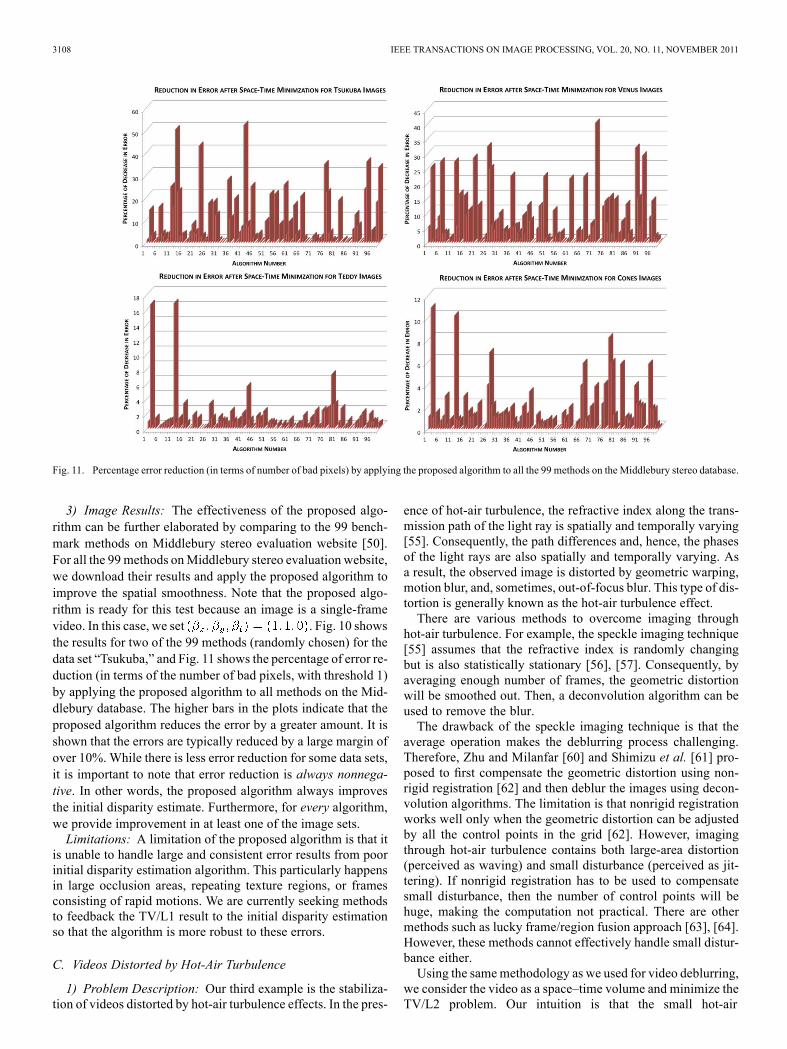
Fig. 11. Percentage error reduction (in terms of number of bad pixels) by applying the proposed algorithm to all the 99 methods on the Middlebury stereo database.

3) Image Results: The effectiveness of the proposed algo-rithm can be further elaborated by comparing to the 99 bench-mark methods on Middlebury stereo evaluation website [50].For all the 99 methods onMiddlebury stereo evaluation website,we download their results and apply the proposed algorithm toimprove the spatial smoothness. Note that the proposed algo-rithm is ready for this test because an image is a single-framevideo. In this case, we set . Fig. 10 showsthe results for two of the 99 methods (randomly chosen) for thedata set “Tsukuba,” and Fig. 11 shows the percentage of error re-duction (in terms of the number of bad pixels, with threshold 1)by applying the proposed algorithm to all methods on the Mid-dlebury database. The higher bars in the plots indicate that theproposed algorithm reduces the error by a greater amount. It isshown that the errors are typically reduced by a large margin ofover 10%. While there is less error reduction for some data sets,it is important to note that error reduction is always nonnega-tive. In other words, the proposed algorithm always improvesthe initial disparity estimate. Furthermore, for every algorithm,we provide improvement in at least one of the image sets.Limitations: A limitation of the proposed algorithm is that it

is unable to handle large and consistent error results from poorinitial disparity estimation algorithm. This particularly happensin large occlusion areas, repeating texture regions, or framesconsisting of rapid motions. We are currently seeking methodsto feedback the TV/L1 result to the initial disparity estimationso that the algorithm is more robust to these errors.

C. Videos Distorted by Hot-Air Turbulence

1) Problem Description: Our third example is the stabiliza-tion of videos distorted by hot-air turbulence effects. In the pres-

ence of hot-air turbulence, the refractive index along the trans-mission path of the light ray is spatially and temporally varying[55]. Consequently, the path differences and, hence, the phasesof the light rays are also spatially and temporally varying. Asa result, the observed image is distorted by geometric warping,motion blur, and, sometimes, out-of-focus blur. This type of dis-tortion is generally known as the hot-air turbulence effect.There are various methods to overcome imaging through

hot-air turbulence. For example, the speckle imaging technique[55] assumes that the refractive index is randomly changingbut is also statistically stationary [56], [57]. Consequently, byaveraging enough number of frames, the geometric distortionwill be smoothed out. Then, a deconvolution algorithm can beused to remove the blur.The drawback of the speckle imaging technique is that the

average operation makes the deblurring process challenging.Therefore, Zhu and Milanfar [60] and Shimizu et al. [61] pro-posed to first compensate the geometric distortion using non-rigid registration [62] and then deblur the images using decon-volution algorithms. The limitation is that nonrigid registrationworks well only when the geometric distortion can be adjustedby all the control points in the grid [62]. However, imagingthrough hot-air turbulence contains both large-area distortion(perceived as waving) and small disturbance (perceived as jit-tering). If nonrigid registration has to be used to compensatesmall disturbance, then the number of control points will behuge, making the computation not practical. There are othermethods such as lucky frame/region fusion approach [63], [64].However, these methods cannot effectively handle small distur-bance either.Using the samemethodology as we used for video deblurring,

we consider the video as a space–time volume and minimize theTV/L2 problem. Our intuition is that the small hot-air


Fig. 12. Hot-air turbulence removal for the sequence “Acoustic Explorer”using the proposed method to reduce the effect of hot-air turbulence. (a) Aframe of the original video sequence. (b) Step 1: Apply GLG [58], [59] to theinput. (c) Step 2: Apply the proposed method to the results of Step 1.

Fig. 13. Zoom-in of “Acoustic Explorer” sequence; frames 25–28 (object is2 mi from the camera). (Top) Input video sequence with contrast enhanced byGLG. (Bottom) Processed video by applying the proposed method to the outputof GLG.

turbulence can be regarded as temporal noise, whereas the ob-ject movement is regarded as temporal edge. Under this frame-work, spatially invariant blur can be also incorporated. If theinput video originally has a low contrast, a preprocessing stepusing gray level grouping (GLG) [58], [59] can be used (SeeFig. 12).2) Experiments: Fig. 13 shows the snapshots (zoom in) of a

video sequence “Acoustic Explorer.” In this example, GLG isapplied to the input videos so that contrast is enhanced. Then,the proposed algorithm is used to reduce the hot-air turbulenceeffect. A Gaussian blur kernel is assumed in both examples,where the variance is empirically determined. Comparing thevideo quality before and after applying the proposed method,fewer jittering such as artifacts are observed in the processedvideos. While this may not be apparent by viewing the still im-ages, the improvement is significant in the 24 fps videos.5

Fig. 14 shows the comparisons without the contrast enhance-ment by GLG. Referring to the figures, the proposed algorithmdoes not only reduce the unstable hot-air turbulence effects, italso improves the blur. The word “Empire State” could not beclearly seen in the input sequence, but it becomes sharper in theprocessed sequence.3) Limitation: The aforementioned experiments indicate

that the proposed algorithm is effective for reducing smallhot-air turbulence effects. However, for large-area geometricdistortions, nonrigid registration is needed. In addition, the gen-eral turbulence distortion is spatially and temporally varying,meaning that the point spread function cannot be modeled asone Gaussian function. This issue is an open problem.

5Videos are available at http://videoprocessing.ucsd.edu/~stanleychan/de-convtv

Fig. 14. Snapshot of “Empire State” sequence. (Left) Input video sequencewithout GLG. (Right) Processed video by applying GLG and the proposedmethod.

V. CONCLUSION

In this paper, we have proposed a video deblurring/denoisingalgorithm that minimizes a TV optimization problem for spa-tial–temporal data. The algorithm transforms the original un-constrained problem to an equivalent constrained problem anduses an augmented Lagrangian method to solve the constrainedproblem. With the introduction of spatial and temporal regular-ization to the spatial–temporal data, the solution of the algorithmis both spatially and temporally consistent.Applications of the algorithm include video deblurring, dis-

parity refinement, and turbulence removal. For video deblur-ring, the proposed algorithm restores motion-blurred video se-quences. The average PSNR is improved, and the spatial andtemporal TVs are maintained at an appropriate level, meaningthat the restored videos are spatially and temporally consistent.For disparity map refinement, the algorithm removes flickeringin the disparity map and preserves the sharp edges in the dis-parity map. For turbulence removal, the proposed algorithm sta-bilizes and deblurs videos taken under the influence of hot-airturbulence.

REFERENCES

[1] R. Gonzalez and R. Woods, Digital Image Processing. EnglewoodCliffs, NJ: Prentice-Hall, 2007.

[2] L. Lucy, “An iterative technique for the rectification of observed dis-tributions,” Astron. J., vol. 79, no. 6, pp. 745–754, Jun. 1974.

[3] W. Richardson, “Bayesian-based iterative method of image restora-tion,” J. Opt. Soc. Amer., vol. 62, no. 1, pp. 55–59, Jan. 1972.

[4] V. Mesarovic, N. Galatsanos, and A. Katsaggelos, “Regularizedconstrained total least-squares image restoration,” IEEE Trans. ImageProcess., vol. 4, no. 8, pp. 1096–1108, Aug. 1995.

[5] P. Hansen, J. Nagy, and D. O’Leary, Deblurring Images: Matrices,Spectra, and Filtering (Fundamentals of Algorithms 3). Philadelphia,PA: SIAM, 2006.

[6] FIJI: Fiji Is Just ImageJ [Online]. Available: http://pacific.mpi-cbg.de/wiki/index.php/Fiji

[7] L. Rudin, S. Osher, and E. Fatemi, “Nonlinear total variation basednoise removal algorithms,” Phys. D, vol. 60, no. 1–4, pp. 259–268,Nov. 1992.

[8] T. Chan, G. Golub, and P. Mulet, “A nonlinear primal-dual method fortotal variation-based image restoration,” SIAM J. Sci. Comput., vol. 20,no. 6, pp. 1964–1977, Nov. 1999.

[9] A. Chambolle, “An algorithm for total variation minimization and ap-plications,” J. Math. Imaging Vis., vol. 20, no. 1/2, pp. 89–97, Jan.–Mar. 2004.

[10] Y. Wang, J. Yang, W. Yin, and Y. Zhang, An efficient TVL1 algo-rithm for deblurring multichannel images corrupted by impulsive noiseCAAM, Rice Univ., Houston, TX, TR-0812, Sep. 2008.


[11] M. Afonso, J. Bioucas-Dias, and M. Figueiredo, “Fast image recoveryusing variable splitting and constrained optimization,” IEEE Trans.Image Process., vol. 19, no. 9, pp. 2345–2356, Sep. 2010.

[12] Y. Wang, J. Ostermann, and Y. Zhang, Video Processing and Commu-nications. Englewood Cliffs, NJ: Prentice-Hall, 2002.

[13] B. Lucas, “Generalized image matching by the method of differences,”Ph.D. dissertation, Carnegie Mellon Univ., Pittsburgh, PA, 1984.

[14] Q. Shan, J. Jia, and A. Agarwala, “High-quality motion deblurring froma single image,” ACM Trans. Graph. (SIGGRAPH), vol. 27, no. 3, pp.73:1–73:10, Aug. 2008.

[15] S. Dai and Y. Wu, “Motion from blur,” in Proc. IEEE CVPR, 2008, pp.1–8.

[16] A. Levin, “Blind motion deblurring using image statistics,” in Proc.NIPS, 2006, pp. 841–848.

[17] S. Cho, Y. Matsushita, and S. Lee, “Removing non-uniform motionblur from images,” in Proc. IEEE ICCV, 2007, pp. 1–8.

[18] J. Jia, “Single image motion deblurring using transparency,” in Proc.IEEE CVPR, 2007, pp. 1–8.

[19] S. Farsiu, D. Robinson, M. Elad, and P. Milanfar, “Fast and robustmulti-frame super-resolution,” IEEE Trans. Image Process., vol. 13,no. 10, pp. 1327–1344, Oct. 2004.

[20] S. Farsiu, M. Elad, and P. Milanfar, “Multi-frame demosaicing andsuper-resolution of color images,” IEEE Trans. Image Process., vol.15, no. 1, pp. 141–159, Jan. 2006.

[21] S. Farsiu, M. Elad, and P. Milanfar, “Video-to-video dynamicsuper-resolution for grayscale and color sequences,” EURASIP J.Appl. Signal Process., vol. 2006, p. 232, 2006.

[22] H. Takeda, S. Farsiu, and P. Milanfar, “Deblurring using regularizedlocally adaptive kernel regression,” IEEE Trans. Image Process., vol.17, no. 4, pp. 550–563, Apr. 2008.

[23] H. Takeda, P. Milanfar, M. Protter, and M. Elad, “Super-resolutionwithout explicit subpixel motion estimation,” IEEE Trans. ImageProcess., vol. 18, no. 9, pp. 1958–1975, Sep. 2009.

[24] M. Ng, H. Shen, E. Lam, and L. Zhang, “A total variation regulariza-tion based super-resolution reconstruction algorithm for digital video,”EURASIP J. Adv. Signal Process., vol. 2007, pp. 1–16, 2007.

[25] S. Belekos, N. Galatsanos, and A. Katsaggelos, “Maximum a posteriorivideo super-resolution using a new multichannel image prior,” IEEETrans. Image Process., vol. 19, no. 6, pp. 1451–1464, Jun. 2010.

[26] S. Chan and T. Nguyen, “LCD motion blur: Modeling, analysis and al-gorithm,” IEEE Trans. Image Process. 2011 [Online]. Available: http://videoprocessing.ucsd.edu/~stanleychan/

[27] B. Jähne, Spatio–Temporal Image Processing: Theory and ScientificApplications. New York: Springer-Verlag, 1993.

[28] Y. Wexler, E. Shechtman, and M. Irani, “Space–time completion ofvideo,” IEEE Trans. Pattern Anal. Mach. Intell., vol. 29, no. 3, pp.463–476, Mar. 2007.

[29] E. Shechtman, Y. Caspi, and M. Irani, “Space–time super-resolution,”IEEE Trans. Pattern Anal. Mach. Intell., vol. 27, no. 4, pp. 531–545,Apr. 2005.

[30] Y. Huang, M. Ng, and Y. Wen, “A fast total variation minimizationmethod for image restoration,” SIAM Multiscale Model Simul., vol. 7,no. 2, pp. 774–795, 2008.

[31] J. Eckstein and D. Bertsekas, “On the Douglas-Rachford splittingmethod and the proximal point algorithm for maximal monotoneoperators,” Math. Program., vol. 55, no. 3, pp. 293–318, Jun. 1992.

[32] J. Douglas and H. Rachford, “On the numerical solution of heat con-duction problems in two and three space variables,” Trans. Amer.Math.Soc., vol. 82, no. 2, pp. 421–439, Jul. 1956.

[33] R. Rockafellar, “Augmented Lagrangians and applications of the prox-imal point algorithm in convex programming,” Math. Oper. Res., vol.1, no. 2, pp. 97–116, May 1976.

[34] R. Rockafellar, “Monotone operators and proximal point algorithm,”SIAM J. Control Optim., vol. 14, no. 5, pp. 877–898, 1976.

[35] M. Tao and J. Yang, Alternating direction algorithms for total variationdeconvolution in image reconstruction Nanjing Univ., Nanjing, China,Tech. Rep. TR0918, 2009 [Online]. Available: http://www.optimiza-tion-online.org/DB_FILE/2009/11/2463.pdf

[36] E. Esser, Applications of Lagrangian-based alternating direc-tion methods and connections to split Bregman UCLA, LosAngeles, CA, Tech. Rep. 09-31, 2009 [Online]. Available:ftp://ftp.math.ucla.edu/pub/camreport/cam09-31.pdf

[37] S. Chan, R. Khoshabeh, K. Gibson, P. Gill, and T. Nguyen, “Anaugmented Lagrangian method for video restoration,” in Proc. IEEEICASSP, 2011.

[38] R. Khoshabeh, S. Chan, and T. Nguyen, “Spatio–temporal consistencyin video disparity estimation,” in Proc. IEEE ICASSP, 2011.

[39] B. Kim, “Numerical optimization methods for image restoration,”Ph.D. dissertation, Dept. Manage. Sci. Eng., Stanford Univ., Stanford,CA, Dec. 2002.

[40] G. Golub and C. Van Loan, Matrix Computation, 2nd ed. Baltimore,MD: Johns Hopkins Univ. Press, 1989.

[41] M. Ng, IterativeMethods for Toeplitz Systems. London, U.K.: OxfordUniv. Press, 2004.

[42] C. Li, “An efficient algorithm for total variation regularization withapplications to the single pixel camera and compressive sensing” M.S.thesis, Dept. Comput. Appl. Math., Rice Univ., Houston, TX, 2009.

[43] A. Levin, A. Rav-Acha, and D. Lischinski, “Spectral matting,” IEEETrans. Pattern Anal. Mach. Intell., vol. 30, no. 10, pp. 1699–1712, Oct.2008.

[44] M. Powell, “A method for nonlinear constraints in minimization prob-lems,” in Optimization, R. Fletcher, Ed. New York: Academic, 1969,pp. 283–298.

[45] T. Goldstein and S. Osher, The split Bregman algorithm for L1 regu-larized problems UCLA, Los Angeles, CA, Tech. Rep. 08-29, 2008.

[46] D. Bertsekas, “Multiplier methods: A survey,” Automatica, vol. 12, no.2, pp. 133–145, Mar. 1976.

[47] M. Choi, N. Galatsanos, and A. Katsaggelos, “Multichannel regular-ized iterative restoration of motion compensated image sequences,” J.Vis. Commun. Image Represent., vol. 7, no. 3, pp. 244–258, Sep. 1996.

[48] C. Paige and M. Saunders, “LSQR: An algorithm for sparse linearequations and sparse least squares,” ACM Trans. Math. Softw., vol. 8,no. 1, pp. 43–71, Mar. 1982.

[49] Y. Lee and T. Nguyen, “Fast one-pass motion compensated frame in-terpolation in high-definition video processing,” in Proc. IEEE ICIP,Nov. 2009, pp. 369–372.

[50] Middleburry Stereo Dataset [Online]. Available: http://bj.middlebury.edu/~schar/stereo/web/results.php

[51] J. Oh, S. Ma, and C. Kuo, “Disparity estimation and virtual view syn-thesis from stereo video,” in Proc. IEEE ISCAS, 2007, pp. 993–996.

[52] J. Fan, F. Liu, W. Bao, and H. Xia, “Disparity estimation algorithm forstereo video coding based on edge detecetion,” in Proc. IEEE WCSP,2009, pp. 1–5.

[53] K. Yoon and I. Kweon, “Locally adaptive support-weight approachfor visual correspondence search,” in Proc. IEEE CVPR, 2005, pp.924–931.

[54] C. Richardt, D. Orr, I. Davies, A. Criminisi, and N. Dodgson,“Real-time spatiotemporal stereo matching using the dual-cross-bilat-eral grid,” in Proc. ECCV, 2010, pp. 510–523.

[55] M. Roggemann and B. Welsh, Imaging Through Turbulence. BocaRaton, FL: CRC Press, 1996.

[56] J. Goodman, Statistical Optics. NewYork:Wiley-Interscience, 2000.[57] J. Goodman, Introduction to Fourier Optics, 4th ed. Englewood, CO:

Roberts & Company Publishers, 2004.[58] Z. Chen, B. Abidi, D. Page, and M. Abidi, “Gray-level grouping

(GLG): An automatic method for optimized image contrast en-hancement—Part I,” IEEE Trans. Image Process., vol. 15, no. 8, pp.2290–2302, Aug. 2006.

[59] Z. Chen, B. Abidi, D. Page, and M. Abidi, “Gray-level grouping(GLG): An automatic method for optimized image contrast enhance-ment—Part II,” IEEE Trans. Image Process., vol. 15, no. 8, pp.2303–2314, Aug. 2006.

[60] X. Zhu and P. Milanfar, “Image reconstruction from videos distortedby atmospheric turbulence,” Vis. Inf. Process. Commun., vol. 7543, no.1, p. 754 30S, 2010.

[61] M. Shimizu, S. Yoshimura, M. Tanaka, and M. Okutomi, “Super-res-olution from image sequence under influence of hot-air optical turbu-lence,” in Proc. IEEE CVPR, 2008, pp. 1–8.

[62] R. Szeliski and J. Coughlan, “Spline-based image registration,” Int. J.Comput. Vis., vol. 22, no. 3, pp. 199–218, Mar./Apr. 1997.

[63] D. Fried, “Probability of getting a lucky short-exposure image throughturbulence,” J. Opt. Soc. Amer., vol. 68, no. 12, pp. 1651–1657, Dec.1978.

[64] M. Aubailly, M. Vorontsov, G. Carhat, and M. Valley, “Automatedvideo enhancement from a stream of atmospherically-distorted images:The lucky-region fusion approach,” Proc. SPIE, vol. 7463, p. 746 30C,2009.


Stanley H. Chan (S’06) received the B.Eng. degreein electrical engineering (with first class honors)from the University of Hong Kong, Pokfulam,Hong Kong, in 2007, and the M.A. degree inapplied mathematics from the University of Cal-ifornia, San Diego (UCSD), La Jolla, in 2009.He is currently working toward the Ph.D. degreein the Department of Electrical and ComputerEngineering, UCSD.His research interests include large-scale convex

optimization algorithms, image and video restora-tion, spatially variant distortion, and space–time signal processing.Mr. Chan is a Croucher Foundation Scholar from 2008 to 2010 and a UCSD

Summer Graduate Teaching Fellow in 2011. He was also the recipient ofthe 2007 Sumida–Yawata Foundation Scholarship, the 2006–2007 Hong KongElectric Company Ltd. Scholarship, the 2004 CLP Scholarship for ElectricalEngineers, and the 2004 Electric Core and Manufacturing Ltd. Scholarship.

Ramsin Khoshabeh (S’08) received the B.S. andM.S. degrees in electrical engineering in 2005 and2007, respectively. He is currently working towardthe Ph.D. degree in the Department of Electrical andComputer Engineering, University of California,San Diego, La Jolla.As an undergraduate, he specialized in computer

design and graduated with highest honors (summacum laude). In graduate school, his emphasis hasbeen on computer vision and 3-D. His thesis workcenters on the application of 3-D in the realm of

surgical practice. His collaborators include two world-renowned surgeons andan expert in digital signal processing, all of which have guided him toward hisacademic goals. His interests include image and video processing, machinelearning, robotics, biology and chemistry, and any opportunities in which hemay help mankind through science and technology.Mr. Khoshabeh was a recipient of California Institute of Telecommunications

and Information Technology Strategic Research Opportunities Fellowship.

Kristofor B. Gibson (S’11) received the B.S. degreefrom Purdue University, West Lafayette, IN, in 2001,the M.S. degree, under the Science, Mathematics,and Research for Transformation Scholarship, in2009 from the University of California, San Diego,La Jolla, where he is also currently working towardthe Ph.D. degree.He has been with Space and Naval Warfare Sys-

tems Center Pacific (SSC Pacific) as a Project En-gineer since 2001 and, more recently, a Video andImage Surveillance Research Engineer. His research

interests are image and video processing and enhancements in addition to com-puter vision algorithms and applications.Mr. Gibson was the recipient of the AFCEA/U.S. Naval Institute 2010 Coper-

nicus Award Winner for the successful development of a video-enhancementcapability for the Navy.

Philip E. Gill received the Ph.D. degree in math-ematics from the Imperial College of Science andTechnology, University of London, London, U.K.,in 1974.He is currently a Distinguished Professor with

the Department of Mathematics, University ofCalifornia, San Diego, La Jolla. He has more than30 years of experience in the development of op-timization algorithms and the production of usablesoftware. He is the coauthor of the computer pack-ages NPSOL and SNOPT that have been distributed

to thousands of universities, research laboratories, and industrial sites aroundthe world. He lists three textbooks on optimization, the most recent of which isNumerical Linear Algebra and Optimization (Addison-Wesley, 1988). He hasmade more than 60 invited presentations at meetings around the world and listsover 100 publications in refereed journals or edited books. He works in the areaof scientific computation, with special reference to numerical optimization.Prof. Gill was the Cochair of the Sixth SIAM Conference on Optimization

held in Atlanta, GA, in 1999. He has served in the Editorial Board for the SIAMJournal on Optimization, which is the SIAM Journal on Matrix Analysis andMathematical Programming Computation, and in the organizing committee ofeight national and international conferences on optimization.

Truong Q. Nguyen (F’05) received the B.S., M.S.,and Ph.D. degrees in electrical engineering from Cal-ifornia Institute of Technology, Pasadena, in 1985,1986, and 1989, respectively.He is currently a Professor with the Department

of Electrical and Computer Engineering, Universityof California, San Diego, La Jolla. He is the coauthor(with Prof. Gilbert Strang) of a popular textbook, i.e.,“Wavelets and Filter Banks” (Wellesley-CambridgePress, 1997), and the author of several MATLAB-based toolboxes on image compression, electrocar-

diogram compression, and filter bank design. His research interests are videoprocessing algorithms and their efficient implementation.Prof. Nguyen is currently the Series Editor (Digital Signal Processing) of

Academic Press. He served as an Associate Editor of the IEEE TRANSACTIONSON SIGNAL PROCESSING from 1994 to 1996, the Signal Processing Lettersfrom 2001 to 2003, the IEEE TRANSACTIONS ON CIRCUITS AND SYSTEMSfrom 1996 to 1997 and from 2001 to 2004, and the IEEE TRANSACTIONS ONIMAGE PROCESSING from 2004 to 2005. He was the recipient of the IEEETRANSACTIONS ON SIGNAL PROCESSING Paper Award (Image and Multidi-mensional Processing area) for the paper that he has coauthored with Prof.P. P. Vaidyanathan on linear-phase perfect-reconstruction filter banks in 1992.He was the recipient of the National Science Foundation Career Award in 1995.

Date post:	29-May-2018
Category:	Documents
Upload:	lamque
View:	216 times
Download:	0 times

IEEE TRANSACTIONS ON IMAGE PROCESSING, VOL. … · optimization problem is solved by transforming...

Documents