IEEE TRANSACTIONS ON MEDICAL IMAGING, … TRANSACTIONS ON MEDICAL IMAGING, VOL. 28, NO. 1, JANUARY...

IEEE TRANSACTIONS ON MEDICAL IMAGING, VOL. 28, NO. 1, JANUARY 2009 137

Nonrigid Registration of Joint Histogramsfor Intensity Standardization in Magnetic

Resonance ImagingFlorian Jäger* and Joachim Hornegger, Member, IEEE

Abstract—A major disadvantage of magnetic resonance imaging(MRI) compared to other imaging modalities like computed to-mography is the fact that its intensities are not standardized. Ourcontribution is a novel method for MRI signal intensity standard-ization of arbitrary MRI scans, so as to create a pulse sequencedependent standard intensity scale. The proposed method is thefirst approach that uses the properties of all acquired imagesjointly (e.g., T1- and T2-weighted images). The image proper-ties are stored in multidimensional joint histograms. In orderto normalize the probability density function (pdf) of a newlyacquired data set, a nonrigid image registration is performed be-tween a reference and the joint histogram of the acquired images.From this matching a nonparametric transformation is obtained,which describes a mapping between the corresponding intensityspaces and subsequently adapts the image properties of the newlyacquired series to a given standard. As the proposed intensitystandardization is based on the probability density functions ofthe data sets only, it is independent of spatial coherence or priorsegmentations of the reference and current images. Furthermore,it is not designed for a particular application, body region oracquisition protocol. The evaluation was done using two differentsettings. First, MRI head images were used, hence the approachcan be compared to state-of-the-art methods. Second, whole bodyMRI scans were used. For this modality no other normalizationalgorithm is known in literature. The Jeffrey divergence of thepdfs of the whole body scans was reduced by 45%. All used datasets were acquired during clinical routine and thus includedpathologies.

Index Terms—General intensity scale, intensity normalization,magnetic resonance imaging (MRI), nonrigid registration, signalintensity standardization, whole body MRI.

I. MOTIVATION

M AGNETIC resonance imaging (MRI) is the preferredimaging modality of the brain and many other body re-

gions due to its excellent soft tissue contrast. Susceptibility ef-fects and local inhomogeneities of the coil system on the other

Manuscript received April 21, 2008; revised July 24, 2008. First publishedAugust 15, 2008; current version published December 24, 2008. This work wassupported by the Erlangen Graduate School in Advanced Optical Technologies(SAOT) by the German National Science Foundation (DFG) in the frameworkof the excellence initiative. Asterisk indicates corresponding author.

*F.Jäger is with the Chair of Pattern Recognition, Friedrich-Alexander-Uni-versity Erlangen-Nuremberg, 91058 Erlangen, Germany (e-mail:[email protected]).

J. Hornegger is with the Chair of Pattern Recognition, Friedrich-Alexander-University Erlangen-Nuremberg, 91058 Erlangen, Germany(e-mail: [email protected]).

Color versions of one or more of the figures in this paper are available onlineat http://ieeexplore.ieee.org.

Digital Object Identifier 10.1109/TMI.2008.2004429

hand can influence signal intensity values. These intensity vari-ations can be separated into two different classes. The first typeof variation (class I) consists of intensities of the same tissueclass which differ throughout a single volume. In literature, thisis called intensity inhomogeneity and is generally caused by again/bias field. In order to deal with this problem, a variety ofalgorithms have been developed in the last decade. All of theseapproaches are based on the assumption that the gain field isvery smooth over the whole image domain, and hence, it doesnot include high-frequency components. A detailed evaluationand summary of many types of algorithms for inhomogeneitycorrection is given in [1]–[3]. The most frequently used methodsare variations of homomorphic unsharp masking [4], [5], whichdirectly utilize the smoothness assumption. More sophisticatedalgorithms either use a segmentation step [6], [7], or make fur-ther statistical assumptions about the shape of the intensity prob-ability distributions of the observed images, or the entropy of theimages [8]–[11].

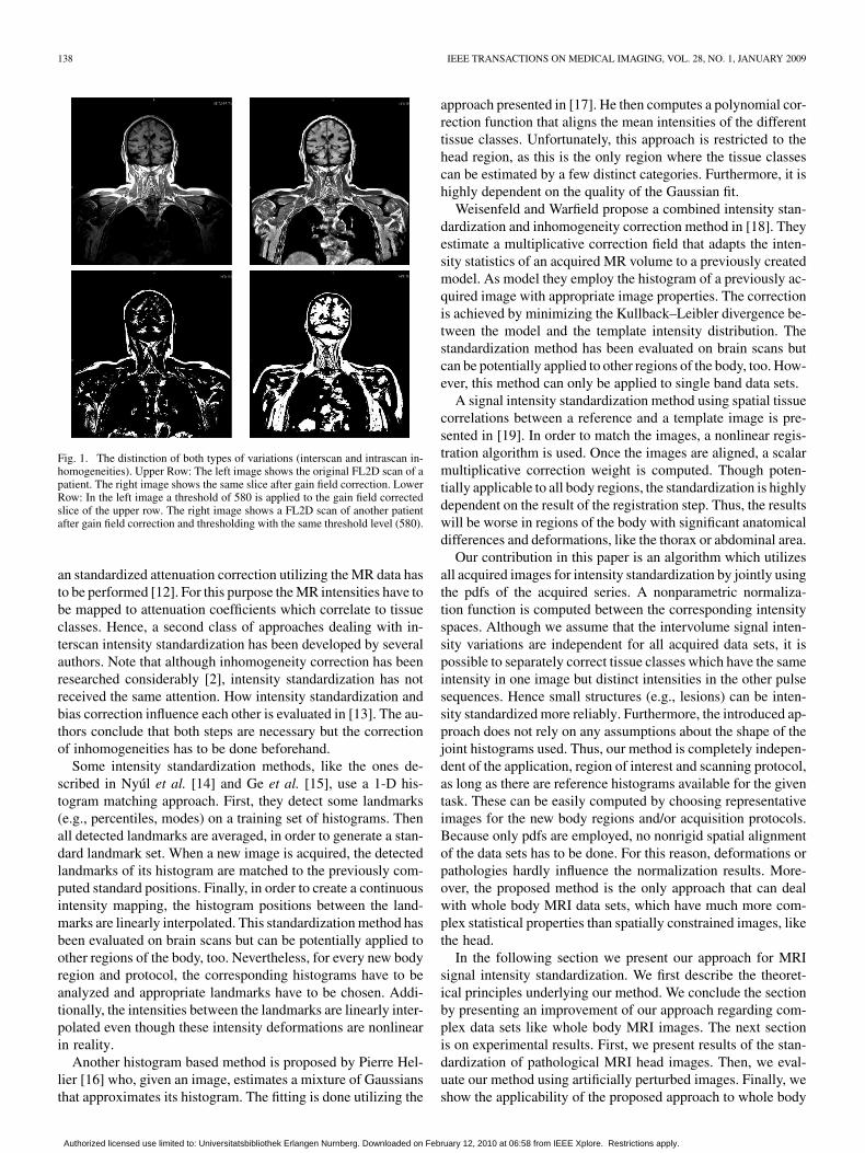
Furthermore, most of these methods do not explicitly solvethe interscan signal intensity variation problem (class II): in-tensities vary between different scans with the same acquisi-tion protocol even for intrapatient studies; thus, a certain mea-sured intensity cannot be associated with a specific tissue class.Solving class II problems is called intensity standardization.After a successful application of an inhomogeneity correctionalgorithm all tissue classes with theoretically identical signalintensities have identical gray values in the images. Unfortu-nately, it is not possible to assign an anatomical meaning to theobserved signal intensities, as these depend on the acquisitionand the applied bias field correction method. The distinction be-tween intensity inhomogeneities and a missing standard signalintensity scale is illustrated in Fig. 1. It can be seen that inho-mogeneity correction algorithms influence the signal intensitieslocally, whereas intensity standardization methods vary intensi-ties globally.

In this paper, we will focus on the class II problem. In gen-eral, a standard intensity scale has no direct impact on medicaldiagnostics by experts; however, volume renderers cannot usestandard presets (transfer functions) to visualize certain organsor tissue classes. The physician has to adjust the settings forevery single scan. Furthermore, more sophisticated automaticsegmentation and quantification methods are needed, as theyhave to adapt their parameters to the observed image intensi-ties. Additionally, currently a new class of hybrid imaging sys-tems combining MR and positron emission tomography (PET)is being developed. In order to increase the PET image quality,

0278-0062/$25.00 © 2008 IEEE

Authorized licensed use limited to: Universitatsbibliothek Erlangen Nurnberg. Downloaded on February 12, 2010 at 06:58 from IEEE Xplore. Restrictions apply.

138 IEEE TRANSACTIONS ON MEDICAL IMAGING, VOL. 28, NO. 1, JANUARY 2009

Fig. 1. The distinction of both types of variations (interscan and intrascan in-homogeneities). Upper Row: The left image shows the original FL2D scan of apatient. The right image shows the same slice after gain field correction. LowerRow: In the left image a threshold of 580 is applied to the gain field correctedslice of the upper row. The right image shows a FL2D scan of another patientafter gain field correction and thresholding with the same threshold level (580).

an standardized attenuation correction utilizing the MR data hasto be performed [12]. For this purpose the MR intensities have tobe mapped to attenuation coefficients which correlate to tissueclasses. Hence, a second class of approaches dealing with in-terscan intensity standardization has been developed by severalauthors. Note that although inhomogeneity correction has beenresearched considerably [2], intensity standardization has notreceived the same attention. How intensity standardization andbias correction influence each other is evaluated in [13]. The au-thors conclude that both steps are necessary but the correctionof inhomogeneities has to be done beforehand.

Some intensity standardization methods, like the ones de-scribed in Nyúl et al. [14] and Ge et al. [15], use a 1-D his-togram matching approach. First, they detect some landmarks(e.g., percentiles, modes) on a training set of histograms. Thenall detected landmarks are averaged, in order to generate a stan-dard landmark set. When a new image is acquired, the detectedlandmarks of its histogram are matched to the previously com-puted standard positions. Finally, in order to create a continuousintensity mapping, the histogram positions between the land-marks are linearly interpolated. This standardization method hasbeen evaluated on brain scans but can be potentially applied toother regions of the body, too. Nevertheless, for every new bodyregion and protocol, the corresponding histograms have to beanalyzed and appropriate landmarks have to be chosen. Addi-tionally, the intensities between the landmarks are linearly inter-polated even though these intensity deformations are nonlinearin reality.

Another histogram based method is proposed by Pierre Hel-lier [16] who, given an image, estimates a mixture of Gaussiansthat approximates its histogram. The fitting is done utilizing the

approach presented in [17]. He then computes a polynomial cor-rection function that aligns the mean intensities of the differenttissue classes. Unfortunately, this approach is restricted to thehead region, as this is the only region where the tissue classescan be estimated by a few distinct categories. Furthermore, it ishighly dependent on the quality of the Gaussian fit.

Weisenfeld and Warfield propose a combined intensity stan-dardization and inhomogeneity correction method in [18]. Theyestimate a multiplicative correction field that adapts the inten-sity statistics of an acquired MR volume to a previously createdmodel. As model they employ the histogram of a previously ac-quired image with appropriate image properties. The correctionis achieved by minimizing the Kullback–Leibler divergence be-tween the model and the template intensity distribution. Thestandardization method has been evaluated on brain scans butcan be potentially applied to other regions of the body, too. How-ever, this method can only be applied to single band data sets.

A signal intensity standardization method using spatial tissuecorrelations between a reference and a template image is pre-sented in [19]. In order to match the images, a nonlinear regis-tration algorithm is used. Once the images are aligned, a scalarmultiplicative correction weight is computed. Though poten-tially applicable to all body regions, the standardization is highlydependent on the result of the registration step. Thus, the resultswill be worse in regions of the body with significant anatomicaldifferences and deformations, like the thorax or abdominal area.

Our contribution in this paper is an algorithm which utilizesall acquired images for intensity standardization by jointly usingthe pdfs of the acquired series. A nonparametric normaliza-tion function is computed between the corresponding intensityspaces. Although we assume that the intervolume signal inten-sity variations are independent for all acquired data sets, it ispossible to separately correct tissue classes which have the sameintensity in one image but distinct intensities in the other pulsesequences. Hence small structures (e.g., lesions) can be inten-sity standardized more reliably. Furthermore, the introduced ap-proach does not rely on any assumptions about the shape of thejoint histograms used. Thus, our method is completely indepen-dent of the application, region of interest and scanning protocol,as long as there are reference histograms available for the giventask. These can be easily computed by choosing representativeimages for the new body regions and/or acquisition protocols.Because only pdfs are employed, no nonrigid spatial alignmentof the data sets has to be done. For this reason, deformations orpathologies hardly influence the normalization results. More-over, the proposed method is the only approach that can dealwith whole body MRI data sets, which have much more com-plex statistical properties than spatially constrained images, likethe head.

In the following section we present our approach for MRIsignal intensity standardization. We first describe the theoret-ical principles underlying our method. We conclude the sectionby presenting an improvement of our approach regarding com-plex data sets like whole body MRI images. The next sectionis on experimental results. First, we present results of the stan-dardization of pathological MRI head images. Then, we eval-uate our method using artificially perturbed images. Finally, weshow the applicability of the proposed approach to whole body


JÄGER AND HORNEGGER: NONRIGID REGISTRATION OF JOINT HISTOGRAMS FOR INTENSITY STANDARDIZATION 139

MRI scans. We have also included a short overview of nonrigidregistration in the Appendix.

II. INTENSITY STANDARDIZATION

The goal of the proposed intensity standardization approachis to find a mapping between the intensities of a -tuple of im-ages , where is the number of imagesacquired with different modalities and a reference -tuple ofimages so that an arbitrary intensityvector describes the same tissue class in both sets with

being the intensity space of the image sets. The mainidea of our method is that this mapping can be approximated bythe minimization of the distance between the joint histograms ofthe two -tuples of images. The required joint histograms are ofdimensionality , corresponding to the number of images. Thedomain of the histograms is . In general, however, it can bescaled to due to the limited number of gray values ob-served. Because of signal intensity outliers, we do not use thefull intensity range but the range up to the 99.8% intensity per-centile. If the difference of the number of gray values in the im-ages is big, then either the scaling of the intensities or the regis-tration parameters have to be adapted for each dimension. Thereason for this is that otherwise the smoothing of the mappingis stronger in the histogram direction with the larger number ofgray values. Note that, at least for real data sets, no plausibletransformation of the relative joint histograms can be found,such that, the difference is zero, because the volume of tissueclasses in the image tuples and differ for interpatient as wellas intrapatient measurements (e.g., anatomical differences, par-tial volume averaging effects, positioning of the patient). Thus,the search for a mapping between the intensity spaces is equiva-lent to finding the transformation between the correspondingjoint histograms which minimizes a given distance measure

(1)

with and being the joint histograms of the imagetuples and . If the joint histograms are treated as images andif there are no constraints on , this task can be viewed as a non-rigid image registration problem. Note that, although in theoryhistograms of arbitrary dimensionality can be used, in practice

should be smaller than five. Otherwise, due to the curse ofdimension, the registration results may be no longer satisfac-tory. Techniques like Parzen estimation can solve the problemof insufficient samples; however, this leads to high computa-tional costs.

For image registration a variety of algorithms are available. Asurvey about image registration is given in Maintz et al. [20] andHill et al. [21]. We employed the variational nonrigid registra-tion approach which was introduced by Modersitzki et al. [22];however, other deformable registrations schemes are applicable,too. The result of this method’s optimization is the transforma-tion . In the context of the registration of multi-dimensional joint histograms, it describes how to transform thegray values of one -tuple of images such that its intensitydistribution best matches the reference distribution, with respect

to the used distance measure and smoother. The objective func-tional of the nonrigid registration can be written as

(2)

with being the distance measure, being a smoother,defining the influence of the smoother on the optimization, and

representing the deformation between the joint histograms.We used the sum of squared differences as distance measureand a curvature based smoother. A more detailed descriptionof nonrigid image registration using a variational frameworkis given in the Appendix. The intensity standardization can bedone by

(3)

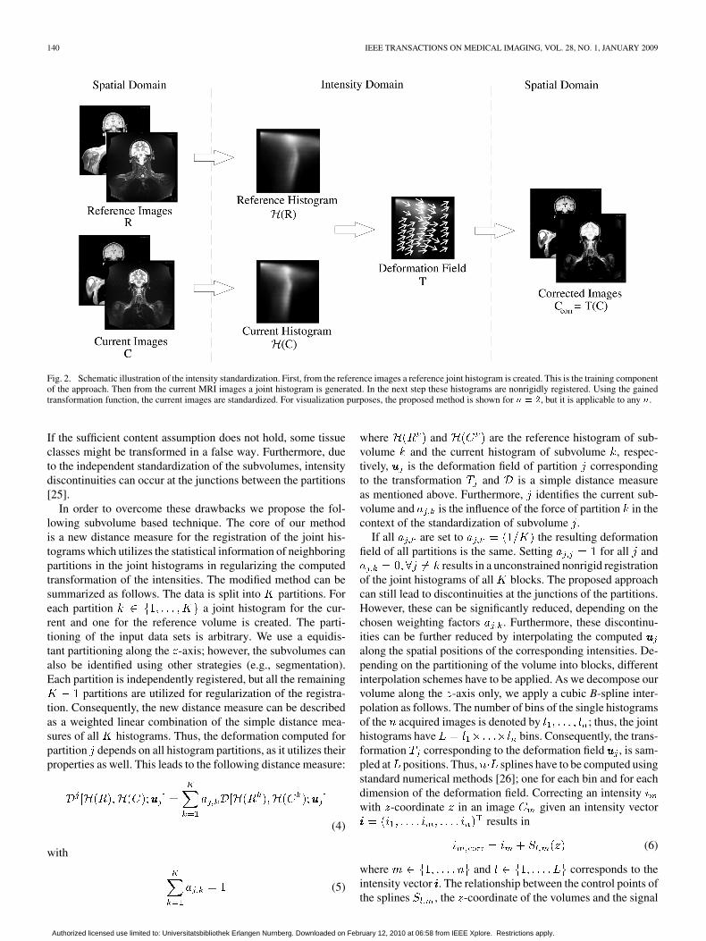
where describes the intensity vector in the originalcurrent image tuple and is the intensity vector inthe corrected images, respectively. A schematic overview of thestandardization process is given in Fig. 2. Here the relationshipbetween the spatial and the intensity domain is illustrated.

If the computed transformation is applied to the joint pdfof the current image tuple, it is not guaranteed that the resultingfunction is still a pdf, as the constraint mightbe invalid. However, as the derived mapping is applied to im-ages, the resulting pdfs will fulfill the constraint again. Never-theless, volume preserving nonrigid registration approaches canbe used as well [23].

In a preprocessing step, the joint histograms were equalized[24]. As the histogram values in areas with small tissue sup-port are very low, the equalization increases the performanceof the registration of these regions by raising the values thereand suppressing values of areas with high tissue support. This isvery important for data sets acquired with protocols that high-light small structures (e.g., blood vessels or kidneys in TIRMimages). Without the equalization step, areas in the joint his-tograms representing such structures are not treated satisfacto-rily in the registration process, as small histogram values hardlyinfluence the distance measure. Thus, the registration concen-trates on structures in the histograms with high tissue support.

For data sets being “statistically simple,” like the head region,the proposed method returns satisfactory results (see SectionIII). However, the following problems may arise in more com-plex data sets: 1) tissue classes with a small number of voxels donot have enough support to be transformed in a reliable manner;2) if a previous bias field correction step has failed, the his-tograms are blurred and the statistical information of a tissueclass is spread to a broad range of gray values. Consequently, itis no longer possible to find a plausible global transformation ofthe intensity vectors. One straightforward solution to this is tosplit the data sets into smaller subvolumes. These subvolumescan then be intensity-standardized separately. However, this canstill lead to problems if the statistical content of a subvolume isnot sufficient for a reliable registration. In order to have suffi-cient statistical content, a partition should have the same dom-inating tissue classes as the corresponding partition in the ref-erence image. Furthermore, the histogram has to have a sim-ilar morphology as the histograms of the neighboring partitions.



Fig. 2. Schematic illustration of the intensity standardization. First, from the reference images a reference joint histogram is created. This is the training componentof the approach. Then from the current MRI images a joint histogram is generated. In the next step these histograms are nonrigidly registered. Using the gainedtransformation function, the current images are standardized. For visualization purposes, the proposed method is shown for � � �, but it is applicable to any �.

If the sufficient content assumption does not hold, some tissueclasses might be transformed in a false way. Furthermore, dueto the independent standardization of the subvolumes, intensitydiscontinuities can occur at the junctions between the partitions[25].

In order to overcome these drawbacks we propose the fol-lowing subvolume based technique. The core of our methodis a new distance measure for the registration of the joint his-tograms which utilizes the statistical information of neighboringpartitions in the joint histograms in regularizing the computedtransformation of the intensities. The modified method can besummarized as follows. The data is split into partitions. Foreach partition a joint histogram for the cur-rent and one for the reference volume is created. The parti-tioning of the input data sets is arbitrary. We use a equidis-tant partitioning along the -axis; however, the subvolumes canalso be identified using other strategies (e.g., segmentation).Each partition is independently registered, but all the remaining

partitions are utilized for regularization of the registra-tion. Consequently, the new distance measure can be describedas a weighted linear combination of the simple distance mea-sures of all histograms. Thus, the deformation computed forpartition depends on all histogram partitions, as it utilizes theirproperties as well. This leads to the following distance measure:

(4)

with

(5)

where and are the reference histogram of sub-volume and the current histogram of subvolume , respec-tively, is the deformation field of partition correspondingto the transformation and is a simple distance measureas mentioned above. Furthermore, identifies the current sub-volume and is the influence of the force of partition in thecontext of the standardization of subvolume .

If all are set to the resulting deformationfield of all partitions is the same. Setting for all and

results in a unconstrained nonrigid registrationof the joint histograms of all blocks. The proposed approachcan still lead to discontinuities at the junctions of the partitions.However, these can be significantly reduced, depending on thechosen weighting factors . Furthermore, these discontinu-ities can be further reduced by interpolating the computedalong the spatial positions of the corresponding intensities. De-pending on the partitioning of the volume into blocks, differentinterpolation schemes have to be applied. As we decompose ourvolume along the -axis only, we apply a cubic B-spline inter-polation as follows. The number of bins of the single histogramsof the acquired images is denoted by ; thus, the jointhistograms have bins. Consequently, the trans-formation corresponding to the deformation field , is sam-pled at positions. Thus, splines have to be computed usingstandard numerical methods [26]; one for each bin and for eachdimension of the deformation field. Correcting an intensitywith -coordinate in an image given an intensity vector

results in

(6)

where and corresponds to theintensity vector . The relationship between the control points ofthe splines , the -coordinate of the volumes and the signal



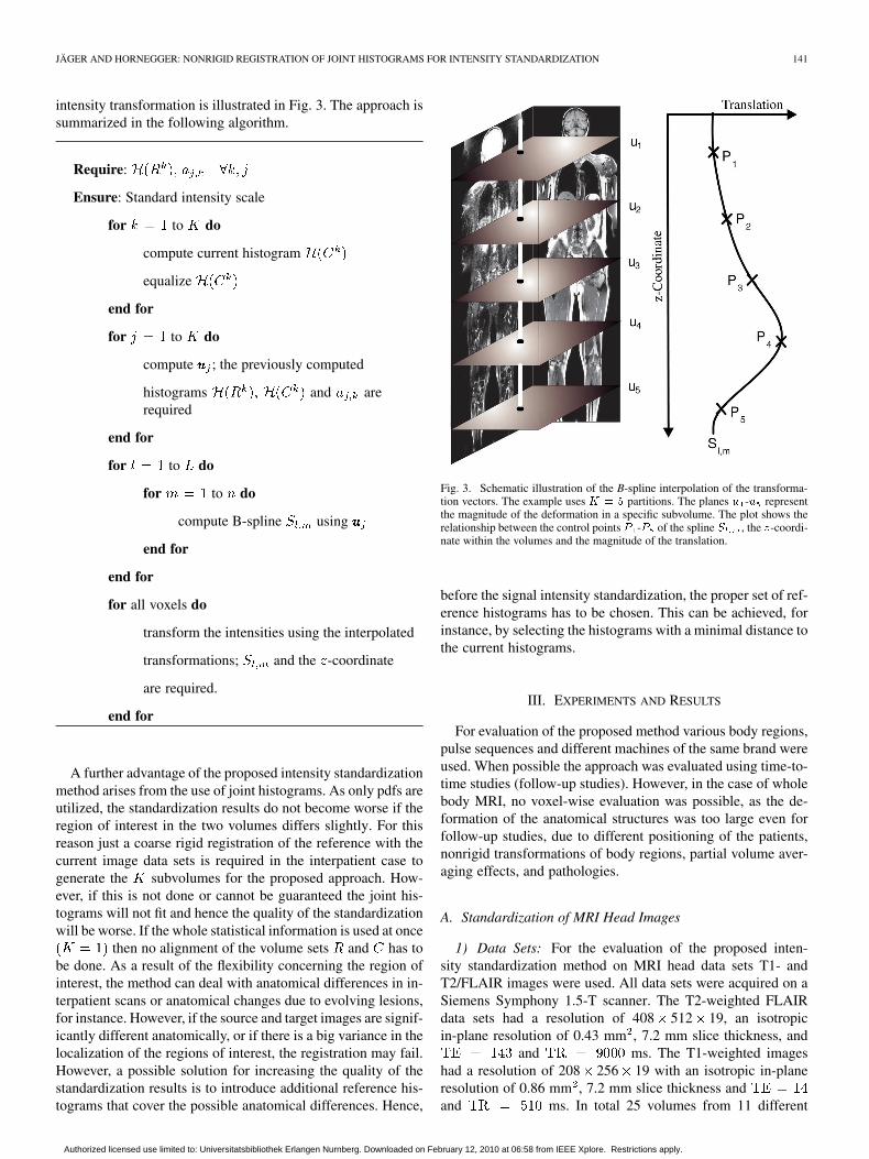
intensity transformation is illustrated in Fig. 3. The approach issummarized in the following algorithm.

Require:

Ensure: Standard intensity scale

for to do

compute current histogram

equalize

end for

for to do

compute ; the previously computed

histograms and arerequired

end for

for to do

for to do

compute B-spline using

end for

end for

for all voxels do

transform the intensities using the interpolated

transformations; and the -coordinate

are required.

end for

A further advantage of the proposed intensity standardizationmethod arises from the use of joint histograms. As only pdfs areutilized, the standardization results do not become worse if theregion of interest in the two volumes differs slightly. For thisreason just a coarse rigid registration of the reference with thecurrent image data sets is required in the interpatient case togenerate the subvolumes for the proposed approach. How-ever, if this is not done or cannot be guaranteed the joint his-tograms will not fit and hence the quality of the standardizationwill be worse. If the whole statistical information is used at once

then no alignment of the volume sets and has tobe done. As a result of the flexibility concerning the region ofinterest, the method can deal with anatomical differences in in-terpatient scans or anatomical changes due to evolving lesions,for instance. However, if the source and target images are signif-icantly different anatomically, or if there is a big variance in thelocalization of the regions of interest, the registration may fail.However, a possible solution for increasing the quality of thestandardization results is to introduce additional reference his-tograms that cover the possible anatomical differences. Hence,

Fig. 3. Schematic illustration of the B-spline interpolation of the transforma-tion vectors. The example uses � � � partitions. The planes � -� representthe magnitude of the deformation in a specific subvolume. The plot shows therelationship between the control points � -� of the spline � , the �-coordi-nate within the volumes and the magnitude of the translation.

before the signal intensity standardization, the proper set of ref-erence histograms has to be chosen. This can be achieved, forinstance, by selecting the histograms with a minimal distance tothe current histograms.

III. EXPERIMENTS AND RESULTS

For evaluation of the proposed method various body regions,pulse sequences and different machines of the same brand wereused. When possible the approach was evaluated using time-to-time studies (follow-up studies). However, in the case of wholebody MRI, no voxel-wise evaluation was possible, as the de-formation of the anatomical structures was too large even forfollow-up studies, due to different positioning of the patients,nonrigid transformations of body regions, partial volume aver-aging effects, and pathologies.

A. Standardization of MRI Head Images

1) Data Sets: For the evaluation of the proposed inten-sity standardization method on MRI head data sets T1- andT2/FLAIR images were used. All data sets were acquired on aSiemens Symphony 1.5-T scanner. The T2-weighted FLAIRdata sets had a resolution of 408 512 19, an isotropicin-plane resolution of 0.43 mm , 7.2 mm slice thickness, and

and ms. The T1-weighted imageshad a resolution of 208 256 19 with an isotropic in-planeresolution of 0.86 mm , 7.2 mm slice thickness andand ms. In total 25 volumes from 11 different



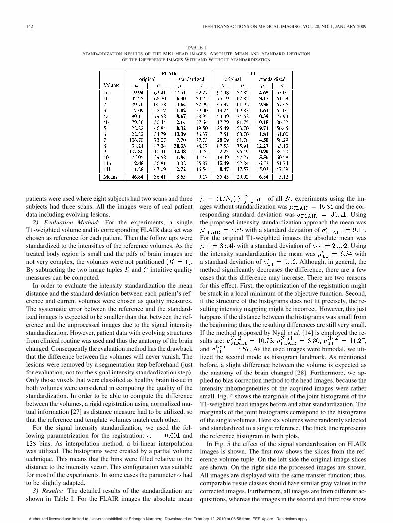
TABLE ISTANDARDIZATION RESULTS OF THE MRI HEAD IMAGES. ABSOLUTE MEAN AND STANDARD DEVIATION

OF THE DIFFERENCE IMAGES WITH AND WITHOUT STANDARDIZATION

patients were used where eight subjects had two scans and threesubjects had three scans. All the images were of real patientdata including evolving lesions.

2) Evaluation Method: For the experiments, a singleT1-weighted volume and its corresponding FLAIR data set waschosen as reference for each patient. Then the follow ups werestandardized to the intensities of the reference volumes. As thetreated body region is small and the pdfs of brain images arenot very complex, the volumes were not partitioned .By subtracting the two image tuples and intuitive qualitymeasures can be computed.

In order to evaluate the intensity standardization the meandistance and the standard deviation between each patient’s ref-erence and current volumes were chosen as quality measures.The systematic error between the reference and the standard-ized images is expected to be smaller than that between the ref-erence and the unprocessed images due to the signal intensitystandardization. However, patient data with evolving structuresfrom clinical routine was used and thus the anatomy of the brainchanged. Consequently the evaluation method has the drawbackthat the difference between the volumes will never vanish. Thelesions were removed by a segmentation step beforehand (justfor evaluation, not for the signal intensity standardization step).Only those voxels that were classified as healthy brain tissue inboth volumes were considered in computing the quality of thestandardization. In order to be able to compute the differencebetween the volumes, a rigid registration using normalized mu-tual information [27] as distance measure had to be utilized, sothat the reference and template volumes match each other.

For the signal intensity standardization, we used the fol-lowing parametrization for the registration: and

bins. As interpolation method, a bi-linear interpolationwas utilized. The histograms were created by a partial volumetechnique. This means that the bins were filled relative to thedistance to the intensity vector. This configuration was suitablefor most of the experiments. In some cases the parameter hadto be slightly adapted.

3) Results: The detailed results of the standardization areshown in Table I. For the FLAIR images the absolute mean

of all experiments using the im-ages without standardization was and the cor-responding standard deviation was . Usingthe proposed intensity standardization approach the mean was

with a standard deviation of .For the original T1-weighted images the absolute mean was

with a standard deviation of . Usingthe intensity standardization the mean was witha standard deviation of . Although, in general, themethod significantly decreases the difference, there are a fewcases that this difference may increase. There are two reasonsfor this effect. First, the optimization of the registration mightbe stuck in a local minimum of the objective function. Second,if the structure of the histograms does not fit precisely, the re-sulting intensity mapping might be incorrect. However, this justhappens if the distance between the histograms was small fromthe beginning; thus, the resulting differences are still very small.If the method proposed by Nyúl et al. [14] is employed the re-sults are: ,and . As the used images were bimodal, we uti-lized the second mode as histogram landmark. As mentionedbefore, a slight difference between the volume is expected asthe anatomy of the brain changed [28]. Furthermore, we ap-plied no bias correction method to the head images, because theintensity inhomogeneities of the acquired images were rathersmall. Fig. 4 shows the marginals of the joint histograms of theT1-weighted head images before and after standardization. Themarginals of the joint histograms correspond to the histogramsof the single volumes. Here six volumes were randomly selectedand standardized to a single reference. The thick line representsthe reference histogram in both plots.

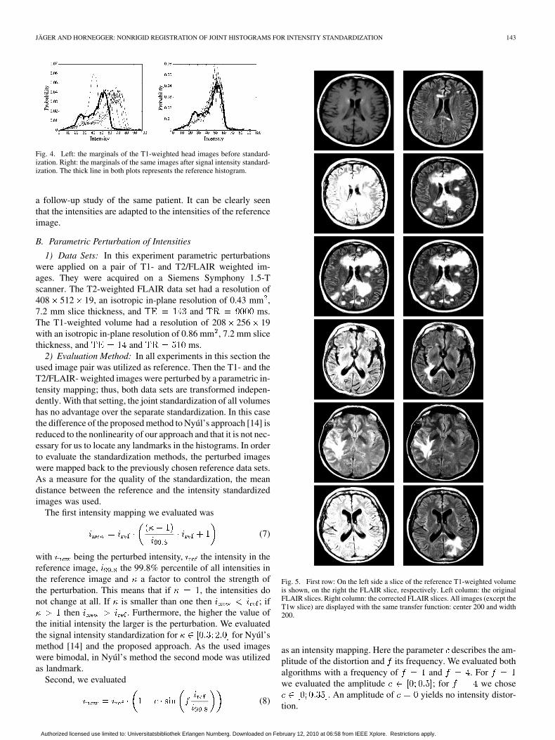
In Fig. 5 the effect of the signal standardization on FLAIRimages is shown. The first row shows the slices from the ref-erence volume tuple. On the left side the original image slicesare shown. On the right side the processed images are shown.All images are displayed with the same transfer function; thus,comparable tissue classes should have similar gray values in thecorrected images. Furthermore, all images are from different ac-quisitions, whereas the images in the second and third row show



Fig. 4. Left: the marginals of the T1-weighted head images before standard-ization. Right: the marginals of the same images after signal intensity standard-ization. The thick line in both plots represents the reference histogram.

a follow-up study of the same patient. It can be clearly seenthat the intensities are adapted to the intensities of the referenceimage.

B. Parametric Perturbation of Intensities

1) Data Sets: In this experiment parametric perturbationswere applied on a pair of T1- and T2/FLAIR weighted im-ages. They were acquired on a Siemens Symphony 1.5-Tscanner. The T2-weighted FLAIR data set had a resolution of408 512 19, an isotropic in-plane resolution of 0.43 mm ,7.2 mm slice thickness, and and ms.The T1-weighted volume had a resolution of 208 256 19with an isotropic in-plane resolution of 0.86 mm , 7.2 mm slicethickness, and and ms.

2) Evaluation Method: In all experiments in this section theused image pair was utilized as reference. Then the T1- and theT2/FLAIR- weighted images were perturbed by a parametric in-tensity mapping; thus, both data sets are transformed indepen-dently. With that setting, the joint standardization of all volumeshas no advantage over the separate standardization. In this casethe difference of the proposed method to Nyúl’s approach [14] isreduced to the nonlinearity of our approach and that it is not nec-essary for us to locate any landmarks in the histograms. In orderto evaluate the standardization methods, the perturbed imageswere mapped back to the previously chosen reference data sets.As a measure for the quality of the standardization, the meandistance between the reference and the intensity standardizedimages was used.

The first intensity mapping we evaluated was

(7)

with being the perturbed intensity, the intensity in thereference image, the 99.8% percentile of all intensities inthe reference image and a factor to control the strength ofthe perturbation. This means that if , the intensities donot change at all. If is smaller than one then ; if

then . Furthermore, the higher the value ofthe initial intensity the larger is the perturbation. We evaluatedthe signal intensity standardization for for Nyúl’smethod [14] and the proposed approach. As the used imageswere bimodal, in Nyúl’s method the second mode was utilizedas landmark.

Second, we evaluated

(8)

Fig. 5. First row: On the left side a slice of the reference T1-weighted volumeis shown, on the right the FLAIR slice, respectively. Left column: the originalFLAIR slices. Right column: the corrected FLAIR slices. All images (except theT1w slice) are displayed with the same transfer function: center 200 and width200.

as an intensity mapping. Here the parameter describes the am-plitude of the distortion and its frequency. We evaluated bothalgorithms with a frequency of and . Forwe evaluated the amplitude ; for we chose

. An amplitude of yields no intensity distor-tion.



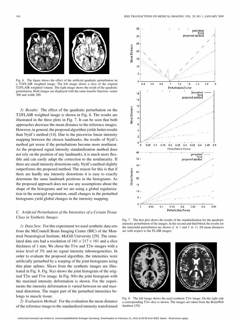
Fig. 6. The figure shows the effect of the artificial quadratic perturbation ona T2/FLAIR weighted image. The left image shows a slice of the originalT2/FLAIR weighted volume. The right image shows the result of the quadraticperturbation. Both images are displayed with the same transfer function: center300 and width 200.

3) Results: The effect of the quadratic perturbation on theT2/FLAIR weighted image is shown in Fig. 6. The results areillustrated in the three plots in Fig. 7. It can be seen that bothapproaches decrease the mean distance to the reference images.However, in general, the proposed algorithm yields better resultsthan Nyúl’s method [14]. Due to the piecewise linear intensitymapping between the chosen landmarks, the results of Nyúl’smethod get worse if the perturbations become more nonlinear.As the proposed signal intensity standardization method doesnot rely on the position of any landmarks, it is much more flex-ible and can easily adapt the correction to the nonlinearity. Ifthere are small intensity distortions only, Nyúl’s method slightlyoutperforms the proposed method. The reason for this is that ifthere are hardly any intensity distortions it is easy to exactlydetermine the same landmark positions in the histograms. Asthe proposed approach does not use any assumptions about theshape of the histograms and we are using a global regulariza-tion in the nonrigid registration, small changes in the perturbedhistograms yield global changes in the intensity mapping.

C. Artificial Perturbation of the Intensities of a Certain TissueClass in Synthetic Images

1) Data Sets: For this experiment we used synthetic data setsfrom the McConnell Brain Imaging Centre (BIC) of the Mon-treal Neurological Institute, McGill University [29]. The simu-lated data sets had a resolution of 181 217 181 and a slicethickness of 1 mm. We chose the T1w and T2w-images with anoise level of 3% and no signal intensity inhomogeneities. Inorder to evaluate the proposed algorithm, the intensities wereartificially perturbed by a warping of the joint histograms usingthin plate splines. Slices from the synthetic images are illus-trated in Fig. 8. Fig. 9(a) shows the joint histogram of the orig-inal T2w and T1w image. In Fig. 9(b) the joint histogram withthe maximal intensity deformation is shown. For the experi-ments the intensity deformation is varied between no and max-imal distortion. The major part of the perturbed intensities be-longs to muscle tissue.

2) Evaluation Method: For the evaluation the mean distanceof the reference image to the standardized intensity transformed

Fig. 7. The first plot shows the results of the standardization for the quadraticintensity perturbation of the images. In the second and third block the results forthe sinusoidal perturbation are shown (� � � and � � �). All mean distancesare with respect to the FLAIR images.

Fig. 8. The left image shows the used synthetic T1w image. On the right sidea corresponding T2w slice is shown. The images are taken from the BrainWebdatabase [29].



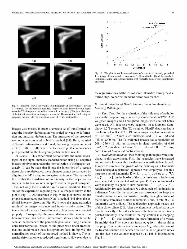
Fig. 9. Image (a) shows the original joint histogram of the synthetic T2w andT1w image. The histogram is equalized for presentation. The �-direction repre-sents the T2w image and the �-direction the T1w image. (b) The joint histogramof the intensity transformed images is shown. (c) The correction result using theproposed method. (d) The correction result of Nyúl’s method [14].

images was chosen. In order to create a set of transformed im-ages the intensity deformation was scaled between no deforma-tion and maximal deformation. The measures of the proposedmethod were compared to Nyúl’s method [14]. Here, we trieddifferent configurations and found, that using the percentile set

where each element represents ath percentile in the histogram yields the best results.3) Results: This experiment demonstrates the main advan-

tages of the signal intensity standardization using all acquiredimages jointly compared to the normalization of the images sep-arately. It can be seen that if just the intensities of a certaintissue class are deformed, these changes cannot be corrected byaligning the 1-D histograms to a given reference. The reason forthis is, that the translation of an intensity in the projection re-sults in the translation of a complete row in the joint histogram.Thus, not only the disturbed tissue class is modified. The re-sult of the experiment regarding the T1w image is shown in theplot of Fig. 10. As illustrated in Fig. 9, the plot shows that theproposed method outperforms Nyúl’s method [14] given the ar-tificial intensity distortion. Fig. 9(d) shows the standardizationresult of the images with maximal intensity deformation. Theintensities of the transformed intensity class were not correctedproperly. Consequently, the mean distances after standardiza-tion are worse than before. Furthermore, streak artifacts can beseen at the borders of the percentile positions. Using a contin-uous transformation instead of the piece-wise linear transfor-mations could reduce these histogram artifacts. In Fig. 9(c) thenormalization result of the proposed method is shown. The in-tensity deformation was reduced significantly. However, due to

Fig. 10. The plot shows the mean distance of the artificial intensity perturbedT1w image, the corrected version using Nyúl’s method [14] and the standard-ized images using the proposed method with respect to the degree of the intensitydistortion.

the regularization and the loss of some intensities during the dis-tortion step, no perfect standardization was reached.

D. Standardization of Head Data Sets Including ArtificiallyEvolving Pathologies

1) Data Sets: For the evaluation of the influence of patholo-gies on the proposed signal intensity standardization T2/FLAIRweighted images and T1 weighted images with contrast boluswere used. All data sets were acquired on a Siemens Sym-phony 1.5 T scanner. The T2-weighted FLAIR data sets had aresolution of 408 512 19, an isotropic in-plane resolutionof 0.43 mm , 7.2 mm slice thickness, and and

ms. The T1-weighted images had a resolution of208 256 19 with an isotropic in-plane resolution of 0.86mm , 7.2 mm slice thickness, and ms,and 14 ml of Magnevist contrast bolus.

2) Evaluation Method: Two evolving pathologies were sim-ulated in this experiment. First, the ventricles were increasedand second, a lesion within the data set was artificially enlarged.In order to simulate the growth of the pathologies, a landmarkbased nonrigid registration approach was employed. For thispurpose a set of landmarks , where

, on the border of the structure (ventricles/lesion)were selected in the treated volume pair . These landmarkswere manually assigned to new positions .Additionally, for each landmark a fixed pair of landmarks ata distance outside the structure was introduced to keep thetransformation as local as possible. Finally, the eight corners ofthe volume were used as fixed landmarks. Thus, in totallandmarks were utilized. The registration approach makes useof thin plate splines [30]. After the alignment the landmarks arematched exactly. The values between the landmarks are inter-polated smoothly. The result of the registration is a mapping

that describes the transformation of a voxel.By multiplying by a constant factor , the resultingmapping generates a new volume pair , where the size ofthe treated structure lies between the size in the original volumesand the size in the volumes mapped by . This is illustrated inFig. 11.



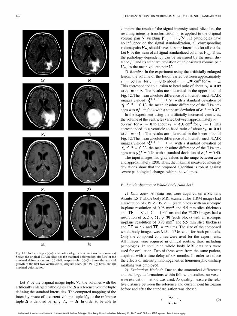
Fig. 11. In the images (a)–(d) the artificial growth of an lesion is shown. (a)Shows the original FLAIR slice, (d) the maximal deformation, (b) 33% of themaximal deformation, and (c) 66%, respectively. (e)–(h) Show the artificialgrowth of the first two ventricles: (e) original slice, (f) 33%, (g) 66%, and (h)maximal deformation.

Let be the original image tuple, the volumes with theartificially enlarged pathologies and a reference volume tupledefining the standard intensities. The computed mapping of theintensity space of a current volume tuple to the referencetuple is denoted by . In order to be able to

compare the result of the signal intensity standardization, theresulting intensity transformation is applied to the originalvolume pair yielding . If pathologies haveno influence on the signal standardization, all correspondingvolume pairs should have the same intensities for all voxels.Let be the mean of all signal standardized volumes . Thus,the pathology dependency can be measured by the mean dis-tance and its standard deviation of an observed volume pair

to the mean volume pair .3) Results: In the experiment using the artificially enlarged

lesion, the volume of the lesion varied between approximatelycm for to about cm for .

This corresponded to a lesion to head ratio of aboutto . The results are illustrated in the upper plots ofFig. 12. The mean absolute difference of all transformed FLAIRimages yielded with a standard deviation of

; the mean absolute difference of the T1w im-ages was with a standard deviation of .

In the experiment using the artificially increased ventricles,the volume of the ventricles varied between approximately

cm for to about cm for . Thiscorresponded to a ventricle to head ratio of aboutto . The results are illustrated in the lower plots ofFig. 12. The mean absolute difference of all transformed FLAIRimages yielded with a standard deviation of

; the mean absolute difference of the T1w im-ages was with a standard deviation of .

The input images had gray values in the range between zeroand approximately 1200. Thus, the maximal measured intensitydeviations show that the proposed algorithm is robust againstsevere pathological changes within the volumes.

E. Standardization of Whole Body Data Sets

1) Data Sets: All data sets were acquired on a SiemensAvanto 1.5 T whole body MRI scanner. The TIRM images hada resolution of (each block) with an isotropicin-plane resolution of 0.98 mm and 5.5 mm slice thicknessand ms and the FL2D images had aresolution of (each block) with an isotropicin-plane resolution of 0.98 mm and 5.5 mm slice thicknessand and ms. The size of the composedwhole body images was for both protocols.Only the composed volumes were used for the experiments.All images were acquired in clinical routine, thus, includingpathologies. In total nine whole body MRI data sets wereused for evaluation. Two of these were from the same patient,acquired with a time delay of six months. In order to reducethe effects of intensity inhomogeneities homomorphic unsharpmasking was employed.

2) Evaluation Method: Due to the anatomical differencesand the large deformations within follow-up studies, no voxel-wise evaluation method was used. As quality measure the rela-tive distance between the reference and current joint histogrambefore and after the standardization was chosen

(9)



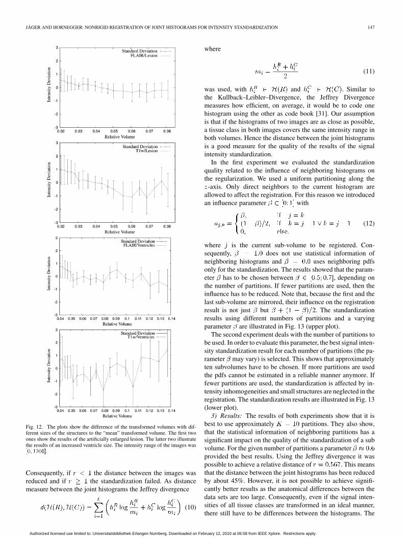
Fig. 12. The plots show the difference of the transformed volumes with dif-ferent sizes of the structures to the “mean” transformed volume. The first twoones show the results of the artificially enlarged lesion. The latter two illustratethe results of an increased ventricle size. The intensity range of the images was�� .

Consequently, if the distance between the images wasreduced and if the standardization failed. As distancemeasure between the joint histograms the Jeffrey divergence

(10)

where

(11)

was used, with and . Similar tothe Kullback–Leibler–Divergence, the Jeffrey Divergencemeasures how efficient, on average, it would be to code onehistogram using the other as code book [31]. Our assumptionis that if the histograms of two images are as close as possible,a tissue class in both images covers the same intensity range inboth volumes. Hence the distance between the joint histogramsis a good measure for the quality of the results of the signalintensity standardization.

In the first experiment we evaluated the standardizationquality related to the influence of neighboring histograms onthe regularization. We used a uniform partitioning along the

-axis. Only direct neighbors to the current histogram areallowed to affect the registration. For this reason we introducedan influence parameter with

(12)

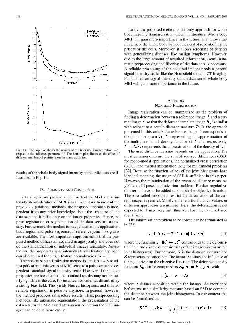
where is the current sub-volume to be registered. Con-sequently, does not use statistical information ofneighboring histograms and uses neighboring pdfsonly for the standardization. The results showed that the param-eter has to be chosen between , depending onthe number of partitions. If fewer partitions are used, then theinfluence has to be reduced. Note that, because the first and thelast sub-volume are mirrored, their influence on the registrationresult is not just but . The standardizationresults using different numbers of partitions and a varyingparameter are illustrated in Fig. 13 (upper plot).

The second experiment deals with the number of partitions tobe used. In order to evaluate this parameter, the best signal inten-sity standardization result for each number of partitions (the pa-rameter may vary) is selected. This shows that approximatelyten subvolumes have to be chosen. If more partitions are usedthe pdfs cannot be estimated in a reliable manner anymore. Iffewer partitions are used, the standardization is affected by in-tensity inhomogeneities and small structures are neglected in theregistration. The standardization results are illustrated in Fig. 13(lower plot).

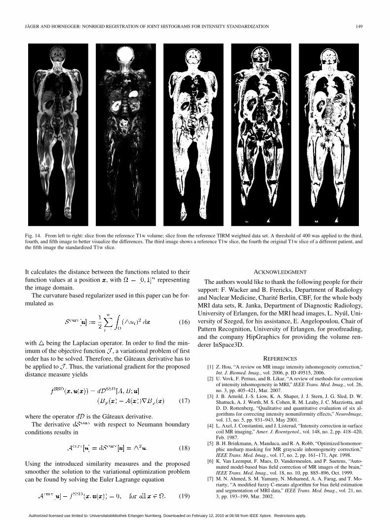
3) Results: The results of both experiments show that it isbest to use approximately partitions. They also show,that the statistical information of neighboring partitions has asignificant impact on the quality of the standardization of a subvolume. For the given number of partitions a parameterprovided the best results. Using the Jeffrey divergence it waspossible to achieve a relative distance of . This meansthat the distance between the joint histograms has been reducedby about 45%. However, it is not possible to achieve signifi-cantly better results as the anatomical differences between thedata sets are too large. Consequently, even if the signal inten-sities of all tissue classes are transformed in an ideal manner,there still have to be differences between the histograms. The



Fig. 13. The top plot shows the results of the intensity standardization withrespect to the influence parameter �. The bottom plot illustrates the effect ofdifferent numbers of partitions on the standardization.

results of the whole body signal intensity standardization are il-lustrated in Fig. 14.

IV. SUMMARY AND CONCLUSION

In this paper, we present a new method for MRI signal in-tensity standardization of MRI scans. In contrast to most of thepreviously published methods, the proposed approach is inde-pendent from any prior knowledge about the structure of thedata sets and it relies only on the image properties. Hence, noprior registration or segmentation of the data sets are neces-sary. Furthermore, the method is independent of the application,body region and pulse sequence, if reference joint histogramsare available. The most important improvement is that the pro-posed method utilizes all acquired images jointly and does notdo the standardization of individual images separately. Never-theless, the proposed signal intensity standardization approachcan also be used for single-feature normalization .

The presented standardization method is a reliable way to ad-just pdfs of multiple series of MRI scans to a pulse sequence de-pendent, standard signal intensity scale. However, if the imageproperties are too distinct, the obtained results may not be sat-isfying. This is the case, for instance, for volumes disturbed bya strong bias field. This yields blurred histograms and thus noreliable registration is possible anymore. In general, however,the method produces satisfactory results. Thus, postprocessingmethods, like automatic segmentation, the presentation of thedata-sets, or the MR based attenuation correction for PET im-ages can be done more easily.

Lastly, the proposed method is the only approach for wholebody intensity standardization known in literature. Whole bodyMRI will gain more importance in the future, as it allows fastimaging of the whole body without the need of repositioning thepatient or the coils. Moreover, it allows screening of patientswith generalizing diseases, like malign lymphoma. However,due to the large amount of acquired information, (semi) auto-matic preprocessing and filtering of the data sets is necessary.A reliable processing of the acquired images needs a generalsignal intensity scale, like the Hounsfield units in CT imaging.For this reason signal intensity standardization of whole bodyMRI will gain more importance in the future.

APPENDIX

NONRIGID REGISTRATION

Image registration can be summarized as the problem offinding a deformation between a reference image and a cur-rent image so that the deformed template image is similarwith respect to a certain distance measure . In the approachpresented in this article the reference image corresponds tothe joint histogram representing an approximation ofthe multidimensional density function of and, respectively,

represents the approximation of the density of .The used distance measure depends on the application. The

most common ones are the sum of squared differences (SSD)for mono-modal applications, the normalized cross correlation(NCC), and mutual information (MI) for multimodal problems[32]. Because the function values of the joint histograms haveidentical meaning, the usage of SSD is sufficient in this paper.However, the minimization of the proposed distance measuresyields an ill-posed optimization problem. Further regulariza-tion terms have to be added to smooth the objective function.These so-called smoothers restrict the deformation of the cur-rent image, in general. Mostly either elastic, fluid, curvature, ordiffusion approaches are utilized. Here, the deformation is notexpected to change very fast, thus we chose a curvature basedregularizer.

The minimization problem to be solved can be formulated asin [22]

(13)

where the function corresponds to the deforma-tion field and is the dimensionality of the images (in this articlejoint histograms). Furthermore, is the distance measure and

represents the smoother. The factor defines the influence ofthe regularizer on the objective function. The deformed densityfunction can be computed as with

(14)

where defines a position within the images. As mentionedbefore, we use a similarity measure based on SSD to computethe distance between the joint histograms. In our context thiscan be formulated as

(15)



Fig. 14. From left to right: slice from the reference T1w volume; slice from the reference TIRM weighted data set. A threshold of 400 was applied to the third,fourth, and fifth image to better visualize the differences. The third image shows a reference T1w slice, the fourth the original T1w slice of a different patient, andthe fifth image the standardized T1w slice.

It calculates the distance between the functions related to theirfunction values at a position , with representingthe image domain.

The curvature based regularizer used in this paper can be for-mulated as

(16)

with being the Laplacian operator. In order to find the min-imum of the objective function , a variational problem of firstorder has to be solved. Therefore, the Gâteaux derivative has tobe applied to . Thus, the variational gradient for the proposeddistance measure yields

(17)

where the operator is the Gâteaux derivative.The derivative with respect to Neumann boundary

conditions results in

(18)

Using the introduced similarity measures and the proposedsmoother the solution to the variational optimization problemcan be found by solving the Euler Lagrange equation

(19)

ACKNOWLEDGMENT

The authors would like to thank the following people for theirsupport: F. Wacker and B. Frericks, Department of Radiologyand Nuclear Medicine, Charité Berlin, CBF, for the whole bodyMRI data sets, R. Janka, Department of Diagnostic Radiology,University of Erlangen, for the MRI head images, L. Nyúl, Uni-versity of Szeged, for his assistance, E. Angelopoulou, Chair ofPattern Recognition, University of Erlangen, for proofreading,and the company HipGraphics for providing the volume ren-derer InSpace3D.

REFERENCES

[1] Z. Hou, “A review on MR image intensity inhomogeneity correction,”Int. J. Biomed. Imag., vol. 2006, p. ID 49515, 2006.

[2] U. Vovk, F. Pernus, and B. Likar, “A review of methods for correctionof intensity inhomogeneity in MRI,” IEEE Trans. Med. Imag., vol. 26,no. 3, pp. 405–421, Mar. 2007.

[3] J. B. Arnold, J.-S. Liow, K. A. Shaper, J. J. Stern, J. G. Sled, D. W.Shattuck, A. J. Worth, M. S. Cohen, R. M. Leahy, J. C. Mazziotta, andD. D. Rottenberg, “Qualitative and quantitative evaluation of six al-gorithms for correcting intensity nonuniformity effects,” NeuroImage,vol. 13, no. 5, pp. 931–943, May 2001.

[4] L. Axel, J. Constantini, and J. Listerud, “Intensity correction in surfacecoil MR imaging,” Amer. J. Roentgenol., vol. 148, no. 2, pp. 418–420,Feb. 1987.

[5] B. H. Brinkmann, A. Manduca, and R. A. Robb, “Optimized homomor-phic unsharp masking for MR grayscale inhomogeneity correction,”IEEE Trans. Med. Imag., vol. 17, no. 2, pp. 161–171, Apr. 1998.

[6] K. Van Leemput, F. Maes, D. Vandermeulen, and P. Suetens, “Auto-mated model-based bias field correction of MR images of the brain,”IEEE Trans. Med. Imag., vol. 18, no. 10, pp. 885–896, Oct. 1999.

[7] M. N. Ahmed, S. M. Yamany, N. Mohamed, A. A. Farag, and T. Mo-riarty, “A modified fuzzy C-means algorithm for bias field estimationand segmentation of MRI data,” IEEE Trans. Med. Imag., vol. 21, no.3, pp. 193–199, Mar. 2002.



[8] W. M. Wells III, W. E. L. Grimson, R. Kikinis, and F. A. Jolesz, “Adap-tive segmentation of MRI data,” IEEE Trans. Med. Imag., vol. 15, no.4, pp. 429–442, Aug. 1996.

[9] B. Likar, M. A. Viergever, and F. Petrus̆, “Retrospective correctionof MR intensity inhomogeneity by information minimization,” IEEETrans. Med. Imag., vol. 20, no. 12, pp. 1398–1410, Dec. 2001.

[10] O. Salvado, C. Hillenbrand, S. Zhang, and D. L. Wilson, “Method tocorrect intensity inhomogeneity in MR images for atherosclerosis char-acterization,” IEEE Trans. Med. Imag., vol. 25, no. 5, pp. 539–552, May2006.

[11] J. G. Sled, A. P. Zijdenbos, and A. C. Evans, “A nonparametericmethod for automatic correction of intensity nonuniformity in MRIdata,” IEEE Trans. Med. Imag., vol. 17, no. 1, pp. 87–97, Feb. 1998.

[12] H. Zaidi, “Is MR-guided attenuation correction a viable option for dual-modality PET/MR imaging?,” Radiology, vol. 244, no. 3, pp. 639–642,Sep. 2007.

[13] A. Madabhushi and J. K. Udupa, “Interplay between intensity standard-ization and inhomogeneity correction in MR image processing,” IEEETrans. Med. Imag., vol. 24, no. 5, pp. 561–576, May 2005.

[14] L. G. Nyúl, J. K. Udupa, and X. Zhang, “New variants of a method ofMRI scale standardization,” IEEE Trans. Med. Imag., vol. 19, no. 2, pp.143–150, Feb. 2000.

[15] Y. Ge, J. K. Udupa, L. G. Nyúl, L. Wei, and R. I. Grossman, “Numer-ical tissue characterization in MS via standardization of the MR imageintensity scale,” J. Magn. Reson. Imag., vol. 12, no. 5, pp. 715–721,Oct. 2000.

[16] P. Hellier, “Consistent intensity correction of MR images,” in Int. Conf.Image Process. (ICIP 2003), Sept. 2003, vol. 1, pp. 1109–12.

[17] K. Van Leemput, F. Maes, D. Vandermeulen, and P. Suetens, “Auto-mated model-based tissue classification of MR images of the brain,”IEEE Trans. Med. Imag., vol. 18, no. 10, pp. 897–908, Oct. 1999.

[18] N. Weisenfeld and S. Warfield, “Normalization of joint image-intensitystatistics in MRI using the Kullback-Leibler divergence,” in IEEE Int.Symp. Biomed. Imag., Arlington, VA, Apr. 2004, pp. 101–104.

[19] M. Schmidt, A method for standardizing MR intensities between slicesand volumes Univ. Alberta, Edmonton, AB, Tech. Rep. TR05-14, 2005.

[20] J. B. A. Maintz and M. A. Viergever, “A survey of medical image reg-istration,” Med. Image Anal., vol. 2, no. 1, pp. 1–36, Mar. 1998.

[21] D. L. G. Hill, P. G. Batchelor, M. Holden, and D. J. Hawkes, “Medicalimage registration,” Phys. Med. Biol., vol. 46, no. 3, pp. R1–R45, Mar.2001.

[22] J. Modersitzki, Numerical Methods for Image Registration. NewYork: Oxford Univ. Press, 2004.

[23] E. Haber and J. Modersitzki, “Numerical methods for volume pre-serving image registration,” Inverse Problems, vol. 20, no. 5, pp.1621–1638, Oct. 2004.

[24] R. C. Gonzalez and R. E. Woods, Digital Image Processing, 2nd ed.Upper Saddle Hill, NJ: Prentice-Hall, 2002.

[25] F. Jäger, L. Nyúl, B. Frericks, F. Wacker, and J. Hornegger, “Wholebody MRI intersity standardization,” in Bildverarbeitung für dieMedizin 2007, A. Horsch, T. Deserno, H. Handels, H. Meinzer, and T.Tolxdorff, Eds. Berlin, Germany: Springer, Mar. 2007, pp. 459–463.

[26] A. Davies and P. Samuels, An introduction to computational geometryfor curves and surfaces. New York: Oxford Univ. Press, 1996.

[27] D. A. Hahn, J. Hornegger, W. Bautz, T. Kuwert, and W. Römer, “Un-biased rigid registration using transfer functions,” Proc. SPIE Med.Imag., vol. 5747, pp. 151–162, 2005.

[28] F. Jäger, Y. Deuerling-Zheng, B. Frericks, F. Wacker, and J.Hornegger, “A new method for MRI intensity standardization withapplication to lesion detection in the brain,” in Vision Model. Vi-sualization, L. Kobbelt, T. Kuhlen, T. Aach, and R. Westermann,Eds. Köln, Germany: AKA GmbH, Nov. 2006, pp. 269–276.

[29] D. Collins, A. Zijdenbos, V. Kollokian, J. Sled, N. Kabani, C. Holmes,and A. Evans, “Design and construction of a realistic digital brainphantom,” IEEE Trans. Med. Imag., vol. 17, no. 3, pp. 463–468, Jun.1998.

[30] K. Rohr, Landmark-Based Image Analysis Using Geometric and Inten-sity Models, ser. Computational Imaging and Vision, M. A. Viergever,Ed. Dordrecht, The Netherlands: Kluwer, 2001.

[31] Y. Rubner, C. Tomasi, and L. J. Guibas, “The earth mover’s distanceas a metric for image retrieval,” Int. J. Comput. Vis., vol. 40, no. 2, pp.99–121, Nov. 2000.

[32] G. Hermosillo, C. Chefd’hotel, and O. Faugeras, “Variational methodsfor multimodal image matching,” Int. J. Comput. Vis., vol. 50, no. 3,pp. 329–343, Dec. 2002.


Date post:	20-Sep-2018
Category:	Documents
Upload:	dothien
View:	215 times
Download:	0 times

IEEE TRANSACTIONS ON MEDICAL IMAGING, … TRANSACTIONS ON MEDICAL IMAGING, VOL. 28, NO. 1, JANUARY...

Documents