IEEE TRANSACTIONS ON PATTERN ANALYSIS AND MACHINE ... -...

IEEE TRANSACTIONS ON PATTERN ANALYSIS AND MACHINE INTELLIGENCE, 1

A morphological approach to curvature-basedevolution of curves and surfaces

Pablo Márquez-Neila, Luis Baumela and Luis Alvarez

Abstract—We introduce new results connecting differential and morphological operators that provide a formal and theoreticallygrounded approach for stable and fast contour evolution. Contour evolution algorithms have been extensively used for boundarydetection and tracking in computer vision. The standard solution based on partial differential equations and level-sets requires theuse of numerical methods of integration that are costly computationally and may have stability issues. We present a morphologicalapproach to contour evolution based on a new curvature morphological operator valid for surfaces of any dimension. We approximatethe numerical solution of the curve evolution PDE by the successive application of a set of morphological operators defined on a binarylevel-set and with equivalent infinitesimal behavior. These operators are very fast, do not suffer numerical stability issues and do notdegrade the level set function, so there is no need of re-initializing it. Moreover, their implementation is much easier since they donot require the use of sophisticated numerical algorithms. We validate the approach providing a morphological implementation of theGeodesic Active Contours, the Active Contours Without Borders and Turpopixels. In the experiments conducted the morphologicalimplementations converge to solutions equivalent to those achieved by traditional numerical solutions, but with significant gains insimplicity, speed and stability.

Index Terms—Computer vision, Mathematical Morphology, Curve Evolution, Level-Sets, Morphological Snakes

✦

1 INTRODUCTION

ACTIVE contours or snakes are one of the mostwidely used computer vision tools [1], [2]. Al-

though they provide a unified account of a numberof visual problems, including detection of edge andsubjective contours [2] and stereo matching [3], theyhave been extensively used for object boundary detec-tion and tracking [1], [2], [4], [5], [6], [7], [8], [9] aswell as segmenting 2D [10], [11], [12], [13], [14] andtensor images [15]. Recent results have shown that theycan achieve robust tracking performance over long andchallenging sequences with dramatic changes in targetshape and appearance [16], [17] as well as overlaps,partial occlusions and poor image contrast [18]. It hasalso been used for oversegmentation [19]. These tasks areformulated in variational terms, where an image inducesan energy functional on a curve or surface. Minimizingthe functional in a steepest descent manner evolves thesurface towards a local minimum that represents thesolution of the problem.

Despite its great success, the original parametric activecontour approach depends on the parametrization ofthe contour and cannot naturally handle changes in

• Pablo Márquez-Neila is with the Departamento de Inteligencia Artificial,Universidad Politécnica de Madrid, Spain.E-mail: [email protected]

• Luis Baumela is with the Departamento de Inteligencia Artificial, Univer-sidad Politécnica de Madrid, Spain.E-mail: [email protected]

• Luis Alvarez is with the Departamento de Informática y Sistemas, Uni-versidad de las Palmas de Gran Canaria, Spain.E-mail: [email protected]

the topology of the curve. These issues were addressedin subsequent approaches such as the Geodesic ActiveContour (GAC) [20], [21] and the Active Contours With-out Edges (ACWE) [10], [11]. In the GAC the energyfunctional is a geodesic in a Riemannian manifold witha metric induced by image features, in its simplestcase, the target borders. The ACWE does not need welldefined borders and it is less sensitive to the initial con-figuration and to the model parameters. Both approachesare based on the level-set formulation [22], [23]. In thiscase the curve is evolved by propagating an interfacerepresented by the zero level-set of a smooth func-tion, using a time-dependent partial differential equation(PDE). The solution to this PDE is costly computation-ally, and in the case of the simplest finite-differenceexplicit numerical scheme, it has stability constraints onthe size of the time step. Absolutely stable solutionsto the GAC model improve the stability by combininga semi-implicit discretization with an additive operatorsplitting (AOS) [24], [25]. Level-set solutions typicallydevelop steep or flat gradients that yield inaccuraciesin the numerical approximation [26]. This is usuallysolved by periodically re-initializing the level-set func-tion as a distance to the zero level-set, which can alsobe addressed as a front propagation problem [27]. Thisagain increases the computational cost of the methodand reduces the topological flexibility, since it preventsthe level-set from creating new contours far away fromthe initial interface [26]. For the ACWE model, however,this re-initiliazation is optional [10].

Both the stability constraints and the necessity ofre-initializing the distance function render traditionallevel-sets approaches as problematic schemes in time-

Digital Object Indentifier 10.1109/TPAMI.2013.106 0162-8828/13/$31.00 © 2013 IEEE

This article has been accepted for publication in a future issue of this journal, but has not been fully edited. Content may change prior to final publication.


critical applications. A considerable number of studiesattempt to alleviate the computational demand reducingthe domain of computation in a narrow band aroundthe zero level-set together with multi-scale techniques,e.g. [25]. Many of the most efficient approaches [9],[12], [28], [29] avoid directly solving the PDE. Theyare based on two key ideas. The curve is implicitlyrepresented by the set of image points neighboring thetarget interface. It is evolved by successive introductionand elimination of points in the interface set. Geometricproperties such as curvature and normal directions to thecurve are approximated using local operations on the setof interface points.

Other approaches to contour evolution try to findglobally optimal solutions. This is possible for the GACmodel when additional constraints are imposed. Forexample, Cohen et al. [30] use as additional constraintsthe locations of the curve end points. The method fromAppleton et al. [31] requires a single point known tobe contained in the area inside the curve. Other recentworks find a convexification of the energy functional viafunctional lifting and convex relaxation [32], [33], [34].The minima of the resulting convex functional coincideswith the global minima. The minimization is based onthe duality of the total variation norm, which is muchfaster than the traditional optimizations based on theEuler-Lagrange equations and it is not sensitive to thesingularities of the level set function. Bresson et al. [32]introduce and globally minimize three new functionals,one closely related to the ACWE model. Their minimiza-tion, based on the duality of the TV-norm, is reportedto be up to 60 times faster than the traditional solutionobtained with the Euler-Lagrange equation.

Despite the additional assumtions that some of theglobal methods require, the advantages of a globally op-timal solution are unquestionable. However, approachesseeking local minima are also of interest in applicationsthat require an intrisically local solution, such as forexample for tracking deformable objects [16], [17] orfor oversegmentation [19]. Moreover, in complex imagesegmentation problems it might be very difficult to finda set of image features and an energy functional whoseglobal optimum is the desired segmentation. This is thecase, for example, in the analysis of Electron Microscopy(EM) images [35], for which user interaction in conjunc-tion with a local approach is presently the best availableapproximation.

Our main goal in this work is to provide a formal,theoretically grounded, approach for stable and fastlocal contour evolution. We base our framework in themathematical morphology. We substitute the terms thatappear in the PDEs of contour evolution algorithms formorphological operators that have equivalent infinitesi-mal behavior. Then, the numerical solution of the PDEis approximated by the successive application of mor-phological operators. The level-set surface is now muchsimpler to define. We assign a value of 0 outside thecontours and 1 inside. These operators are very fast, do

not suffer numerical stability issues and do not degradethe level set function, so no re-initialization is required.Moreover, their implementation is much easier sincethey do not require the use of sophisticated numericalalgorithms.

To formally support our solution we introduce new re-sults that relate differential and morphological operators.The connection between differential and morphologicaloperators has also been studied before. Lax was the firstto use multi-scale dilations and erosions to give stableand efficient numerical schemes for solving PDEs [36].Later it was rediscovered by several authors [37], [38].Now, it is well-known that the PDE evolution rule whichdescribes a curve moving along its normal behaves likethe morphological operators dilation and erosion actingon the level set function [39]. However, not all PDEs haveequivalent morphological operators. The most importantPDE contour evolution rule, the mean curvature evolu-tion [39], [40], has no known morphological equivalentoperator. The importance of curvature-based evolutionlies on the fact that it commonly appears in most PDE-based algorithms as a regularizing term. Hence theinterest in finding a morphological equivalent. In thisdirection, some advances were achieved by Catté, Dibosand Koepfler proving that the mean curvature evolutionfor planar curves can be replaced by the mean of twomorphological operators [41].

Our work has several contributions. First, we intro-duce a curvature morphological operator that can beused for curve evolution. Second, we prove that ouroperator can be generalized to higher dimensions and,therefore, it can be used for the evolution of curves,surfaces and hyper-surfaces of any dimension. Third,we show how the composition of different morpho-logical operators approximates the numerical solutionof PDEs for hyper-surface evolution, with significantgains in simplicity, speed, and stability. Specifically, weintroduce morphological versions of the Turbopixels su-persegmentation algorithm and two of the most popularcurve evolution algorithms, the Geodesic Active Contours(GAC) [20] and Chan and Vese’s Active Contours WithoutEdges (ACWE) [10].

In [42] we presented a morphological approach to theevolution of 2D contours based on which we introducedthe Morphological GAC. Here we generalize this resultto surfaces of any dimension, introduce theMorphologicalActive Contours Without Edges (Morphological ACWE),the Morphological Turbopixels and perform a larger set ofexperiments.

The rest of the paper is organized as follows. In Sec-tion 2 we present background knowledge about differ-ential equations and morphological operators. Section 3introduces the curvature morphological operator andstudies its behavior in 2D, 3D and n-dimensional cases.We introduce theMorphological Snakesmodel in Section 4.Some implementation details are given in Section 5.Finally, we perform experimental analysis and drawconclusions in Sections 6 and 7.



2 BACKGROUND

In this section we briefly review both explicit and im-plicit curve and surface evolution, morphological oper-ators and the relation between PDEs and morpholog-ical operators. The interested reader may consult [39]for §2.1, [40] for §2.2 and [41] for the last part of §2.3.

2.1 PDEs and contour evolution

Differential operators are fundamental tools in the com-puter vision and graphics communities. They are usedin a variety of tasks such as determining the length ofgeodesic curves and computing the curvature of surfacesor smoothing meshes. Differential operators are key tocontour evolution with PDEs [39], [40], where the in-finitesimal change of a contour is given by a differentialoperator. We begin by recalling some information aboutcurve evolution.

Let C : R+ × [0, 1] → R

2 : (t, p) → C(t, p) be aparametrized 2D curve over time. A differential oper-ator L defines the curve evolution with the PDE Ct =L(C). Different forms of L result in different types ofevolution. It is not difficult to see that every L can berewritten as L(C) = F ·N , where N is the normal to thecurve and F is a scalar field —possibly depending onthe curve— which determines the velocity of evolutionof each point in the curve.

Out of all the possible forms that L can take, a feware of special interest for their theoretical properties andbecause they have been extensively used. First, L maybe defined as the normal to the curve (i.e., F ∈ {1,−1}),Ct = N or Ct = −N . Here, the curve moves alongits normal direction with constant velocity. Second, ifL(C) = KN (i.e., F = K), we get the intrinsic heat equa-tion [40], Ct = KN , where K is the Euclidean curvatureof C. The curvature flow given by this expression takesarbitrary non-intersecting curves and evolves them intoconvex ones. Then, it evolves convex curves into circularcurves which converge to a point [39].In many contexts it is unusual to work with an explicit

representation of the curve. When C is explicit, it is noteasy to deal with topological changes like merge andsplit, and a re-parametrization of the curve may be re-quired. The Osher-Setian [22] level set method fixes thisby representing the curve implicitly as a level set of anembedding function. Let u : R+×R

2 → R be an implicitrepresentation of C such that C(t) = {(x, y);u(t, (x, y)) =0}. If the curve evolution has the form Ct = F · N ,the evolution of any function u(x, y) which embeds the

curve as one of its level sets is∂u

∂t= F · |∇u| [22], [39].

In the level-set framework, the previous PDEs forcurve evolution are

∂u

∂t= ±|∇u| (1)

when F = ±1 and

∂u

∂t= div

(∇u

|∇u|

)· |∇u| (2)

when F = K, since the divergence of the normalizedgradient gives the curvature of the implicit curve at eachpoint.

Most existing results for curve evolution also apply tothe case of surface evolution. The explicit representationof an evolving surface is a map S : R+×[0, 1]2 → R

3. Theevolution rule of a surface has the form St = FN , whereF is a scalar field and N is the normal to the surfaceat each point. The previous curve evolution approacheshave equivalent versions for surfaces when F = ±1 orF = H, where H is the mean curvature of the surface.The extension of the level-set framework to the implicitsurface evolution is straightforward. Consider the scalarfield u : R+×R3 → R. A surface S is implicitly defined asa level set of u. The expressions for the implicit surfaceevolution coincide with equation (1) when F = ±1 andwith equation (2) when F = H. Equation (2) definedfor the general n-dimensional case is known as the meancurvature motion.

2.2 Morphological operators

Monotone contrast-invariant and translation-invariantoperators are called morphological operators. The mostcommon ones are the dilation and the erosion operators.A dilation Dh with radius h of function u is defined as

Dhu(x) = supy∈hB(0,1)

u(x+ y), (3)

while the erosion has a similar form

Ehu(x) = infy∈hB(0,1)

u(x+ y). (4)

In both definitions, B(0, 1) is the ball of radius 1 centeredat 0 and the term hB is the set B scaled by h, i.e., hB ={hx : x ∈ B}.

An interesting result in mathematical morphology isthat every morphological operator T admits a sup-infrepresentation of the form

(Thu)(x) = supB∈B

infy∈x+hB

u(y) (5)

or a dual inf-sup representation

(Thu)(x) = infB∈B

supy∈x+hB

u(y). (6)

In both cases, B is a set of structuring elements thatuniquely defines the operator, and h is the size of theoperator.

For example, choosing a proper B one may expressdilations and erosions in a sup-inf or inf-sup form. Thedilation with radius h admits an inf-sup form when B ismade of the single structuring element, B = {B(0, 1)}.Similarly, the erosion has an sup-inf form using the samebase.



2.3 From PDEs to morphological operators

Some morphological operators can be expressed asPDEs. The key idea to find these connections is tostudy the behavior of the successive application of amorphological operator with a very small radius. In thissection we review some of these relations.

The dilation Dh verifies that [37]

limh→0+

Dhu− u

h= |∇u|. (7)

This means that the successive application of Dh withvery small radius, limm→∞(Dt/m)mu0, is equivalent tothe solution of

∂u

∂t= |∇u| (8)

with initial value u(0,x) = u0(x). We say that the dilationhas an infinitesimal behavior equivalent to the PDE (8).

The erosion presents a similar property, since [37]

limh→0+

Ehu− u

h= −|∇u|, (9)

and therefore the erosion has an infinitesimal behaviorequivalent to the PDE

∂u

∂t= −|∇u| (10)

Thanks to this behavior, we can approximate the level-set evolution PDEs (1) using the successive applicationof the morphological operators Dh and Eh.

3 THE CURVATURE MORPHOLOGICAL OPERA-TOR

In this section we introduce a new curvature morpho-logical operator that can be used to evolve curves em-bedded in spaces of any dimension.

3.1 The 2D curvature morphological operator

Let SIh and ISh be respectively the sup-inf and inf-sup morphological operators given by the base B2 ={[−1, 1]θ ⊂ R

2 : θ ∈ [0, π)} made of all segments oflength 2 centered at the origin. In their pioneering work,Catté, Dibos and Koepfler proved that the successiveapplication of the mean operator, F√

h, for a very small his equivalent to the curvature flow of the PDE (2) [41],where

(Fhu)(x) =(SI2h u)(x) + (IS2h u)(x)

2. (11)

Unfortunately, operator Fh is not contrast-invariantand hence it is not a morphological operator. We avoidthis problem using operator composition.

Lemma 3.1. Let T 1h and T 2

h be two morphological operators,we have, for a small h, that

T 2h/2 ◦ T

1h/2u ≈

T 2hu+ T 1

hu

2. (12)

Proof: Let L1h and L2

h be the corresponding infinites-imal operators of morphological operators T 1

h and T 2h .

We can write a first order approximation to the operatorcomposition T 2

h/2 ◦ T1h/2 as

T 2h/2 ◦ T

1h/2u ≈ T 2

h/2

(u+

h

2L1h(u)

)

≈ u+h

2L1h(u) +

h

2L2h(u) +

+

(h

2

)2

L2hL

1h(u).

The last term depends on the squared value of h, and itcan be dismissed for a small h,

T 2h/2◦T

1h/2u ≈

u+ hL1h(u)

2+u+ hL2

h(u)

2≈

1

2(T 2

hu+T 1hu).

The approximation in (12) is accurate for small valuesof h. In this case we can replace 1

2 (T2hu + T 1

hu) by thecomposition T 2

h/2 ◦ T1h/2u. Then, the non-morphological

operator F√h can be approximated by the composi-

tion SI√h ◦ IS√h.

Definition 3.2. The curvature morphological operator isdefined as SI√h ◦ IS

√h.

3.2 The d-dimensional curvature morphological op-erator

Here we generalize the curvature morphological opera-tor to hyper-surfaces of any dimension. In this case theembedding function is defined as u : Rd → R, and itslevel sets are (d − 1)-hypersurfaces. The d-dimensionalmorphological operators SIh and ISh are, respectively,the sup-inf and inf-sup operators with the new base Bd,made up of all hyper-disks of radius 1 centered at theorigin, Bd = {Kn : n ∈ Sd−1}, where Sd−1 = {n ∈ R

d :‖n‖ = 1} and Kn = {v ∈ R

d :‖v‖ ≤ 1,vTn = 0}.The effect of the mean operator (SIh + ISh)/2 over

the hyper-surfaces of u is explained by the followingTheorem,

Theorem 3.3. The d-dimensional operator Fh has an in-finitesimal behavior given by

limh→0+

(F√hu)− u

h= (min(κ1, . . . , κd−1, 0)

+max(κ1, . . . , κd−1, 0)) · |∇u|,

where κi, 1 ≤ i ≤ d − 1 are the principal curvatures of thehyper-surface implicitly defined by u at each point.

Proof: The projection matrix associated to a vec-tor n ∈ Sd−1 is Pn = Id − nnT , where Id is theidentity d × d matrix. Pn projects any vector w to ahyperplane orthogonal to n. We can easily deduce thatKn = {Pnw : w ∈ Sd−1}.To study the effect of the operators, we expand u using

Taylor series up to second order:

u(x+ hw) = u(x) + h∇u(x)Tw +h2

2wTD2(x)w + o(h3),



where D2(x) is the Hessian matrix of u at x. If we wantto restrict the Taylor expansion to the orthogonal planeto a given vector n ∈ Sd−1 we can use the projectionmatrix Pn. That is,

u(x+hPnw) = u(x)+h∇u(x)TPnw+h2

2wTPnD

2(x)Pnw+o(h3).

A case of special interest is ng = ∇u(x)‖∇u(n)‖ , which cor-

responds to the analysis of the geometric properties ofthe level set surface at x. In this case, the above Taylorexpansion can be expressed as

u(x+ hPngw) = u(x) +

h2

2wTPng

D2(x)Pngw + o(h3).

Note that the first order term cancels since Pngw is

orthogonal to ∇u(x). Matrix M = PngD2(x)Png

is a d×dmatrix with d eigenvalues. One of them is λ0 = 0 whichcorresponds to the eigenvector ng . The d−1 eigenvectorsλi, 1 ≤ i ≤ d − 1 are closely related to the principalcurvatures κi of the implicit hyper-surface at x:

λi = κi · |∇u(x)|. (13)

See the Chapter 11 of [40] for details. A straightforwardcomputation leads to

supy∈x+hKng

u(y) = supw∈Sd−1

u(x+ hPngw) (14)

= u(x) +h2

2max(λ1, . . . , λd−1, 0) + o(h3),

infy∈x+hKng

u(y) = infw∈Sd−1

u(x+ hPngw) (15)

= u(x) +h2

2min(λ1, . . . , λd−1, 0) + o(h3).

We will prove that the supreme of the infimum for theSIh operator is attained at ng , so that

SIhu(x) = supn∈S(d−1)

infy∈hKn

u(y) = infy∈x+hKng

u(y).

Let us denote by nh ∈ Sd−1 an orthogonal directionwhere

supn∈S(d−1)

infy∈hKn

u(y) = infy∈x+hKnh

u(y). (16)

Note that since Sn−1 is a compact set and n →infy∈hKn

u(y) is a continuous function, then nh alwaysexists. We will show that

limh→0

nh = ng. (17)

To prove the equality we assume the opposite, that is,there exists ε > 0 such that for each m ∈ N there existsnhm

∈ Sd−1 with ‖nhm−ng‖ > ε and |hm| <

1m . We will

show that if hm is small enough, then

infy∈x+hKnhm

u(y) < infy∈x+hKng

u(y) (18)

which is in contradiction with the definition of nh in (16).We observe that the above inequality is equivalent to

infw∈Sn−1

(∇u(x)TPnhm

w +hm

2wTPnhm

D2(x)Pnhmw + o(h2

m)

)

< infw∈Sn−1

(hm

2wTPng

D2(x)Pngw + o(h2

m)

).

When hm goes to 0, the right part of the above inequalitygoes to 0 too. However, in the left hand side, we observethat if we choose w = ng then ∇u(x)TPnh∞

ng = ε′ > 0since ‖nhm

−ng‖ > ε. Therefore, the left hand side holdsthat

infw∈Sn−1

(∇u(x)TPnhm

w +hm

2wTPnhm

D2(x)Pnhmw + o(h2

m)

)

≤ −ε′ +hm

2nTg Pnhm

D2(x)Pnhmng + o(h2

m).

If hm is small enough, the right part of the aboveinequality is strictly lower than 0, and (18) is satisfied.This is in contradiction with the definition of nh, andtherefore (17) is true.We can use the same argument for the operator ISh:

when h goes to 0, the infimum is attained in the planeorthogonal to the gradient. Therefore, when h is small,the operators SIh and ISh behave as given in theexpressions (14) and (15). Using these expressions, themean operator Fh

Fhu(x) =(SI2h u)(x) + (IS2h u)(x)

2

can be written as

Fhu(x) = u(x) + h2(min(λ1, . . . , λd−1, 0)

+max(λ1, . . . , λd−1, 0)) + o(h3).

Reorganizing terms and substituting the eigenvaluesof M according to (13), we obtain that

limh→0+

F√hu(x)− u(x)

h= (min(κ1, . . . , κd−1, 0)

max(κ1, . . . , κd−1, 0)) · |∇u|.

Corollary 3.4. The 2D operator Fh has an infinitesimalbehavior given by

limh→0+

(F√hu)− u

h= κ · |∇u| = div

(∇u

|∇u|

)· |∇u|. (19)

Proof: Trivial from Theorem 3.3.This is the result that Catté, Dibos and Koepfler proved

in [41]. Here we have shown that it is a special caseof the more general Theorem 3.3. In consequence, thesuccessive application of the curvature morphologicaloperator, SI√h ◦ IS

√h, with base B2 is equivalent to the

solution of PDE (2).



n

nnnnnnnnnnnnnnKnnKnKKnKKnKKKnKKnKKKKnKKnKKKKKKnnKKKKKKKKKKKKKKKKKKKKKKKKKKKKKKKKKKKKKKKKKKKKKKKKKKKKKKKKKKKKKKKKKKKKK

n

nnnnnnnnnnKnnKnnKnnKnKnnKKnKKKnKKKnKKKnKKKKnKKnKKKKnKKKnKKnKKKKnKKKKKKKKKKKKKKKKKKKKKKKKKKKKKKKKKKKKKKKKKKKKKKKKKKKKKKKKK n nnnnnnnnnnnnnnnnnnn nnnn nnnn KnKKKnKnn KKKnKnn KKnn KKKKn KKn KKKn KKn KKKn KKn KKKKKKKKKKn Kn KKKKKKKKKKKKKn KKn KKKKKKKn KKnnn KKKKKKKKn Kn KKKKKKn KKn KKKKKKKKn KKn KKKKKKn KKn KKKKKKn Kn KKKKn KKn KKKKKn KKn KKKn Kn KKKKnn KKKnn KKKKKKKKKKKKKKKKKKKKK

Fig. 1. The base B3 for the 3D SIh and ISh operators ismade up of all disks with radius 1 centered at the origin.The figure depicts three of those disks marked in blue.Each disk Kn is determined by its normal n.

3.3 The 3D curvature morphological operator

Although we extended in section 3.2 the definition of thecurvature morphological operator to the n-dimensionalcase, practical applications will typically use the 2D and3D versions to process respectively images and imagestacks. In the experiments section we study these twocases. So, for completeness, here we consider the 3Dcurvature morphological operator and compare it withthe well-known mean curvature motion PDE.

Operators SIh and ISh may also be expressed in the3D case. We define the new base as the set of all disksof radius 1 centered at the origin B3 = {Kn : n ∈ S2},where S2 = {n ∈ R

3 : ‖n‖ = 1} is the 2-sphere ofradius 1 and Kn = {v ∈ R

3 : ‖v‖ ≤ 1,vTn = 0} is thedisk of radius 1 centered at the origin and orthogonalto n. Figure 1 shows some elements of B3. Now we canstate the following

Corollary 3.5. The 3D operator Fh has the infinitesimalbehavior

limh→0+

(F√hu)− u

h= (min(κ1, κ2, 0)+max(κ1, κ2, 0))·|∇u|,

where κ1 and κ2 are the principal curvatures of the surfaceimplicitly defined by u at each point.

Proof: Trivial from Theorem 3.3.Let us now compare the infinitesimal behavior of the

3D operator Fh with the mean curvature motion PDE (2)in 3D. Recall that the term div

(∇u|∇u|

)is equivalent to

the mean curvature H = κ1 + κ2 of the implicit surface.Therefore, the mean curvature motion may be rewrittenas

∂u

∂t= (κ1 + κ2) · |∇u|. (20)

Corollary 3.5 relates the evolution providedby SI√h ◦ IS

√h with the evolution of PDE

∂u

∂t= (min(κ1, κ2, 0) + max(κ1, κ2, 0)) · |∇u|. (21)

Comparing PDEs (20) and (21) we can immediatelyconclude that the evolution provided by the curvaturemorphological operator is not strictly equivalent to themean curvature flow. We can distinguish two cases. First,

Fig. 2. The base P for the 2D discrete SId ◦ ISd operator.

if both principal curvatures have the same sign (e.g., asphere) and assuming that |κ2| ≥ |κ1|, (21) becomes

∂u

∂t= κ2 · |∇u|.

This is equivalent to the mean curvature motion if κ1 =0. As |κ1| gets larger, the difference between both flowsbecomes more noticeable. However, the sign of the flowis the same in both equations. In the second case, theprincipal curvatures have different sign (e.g., a catenoid).Then, (21) becomes

∂u

∂t= (κ1 + κ2) · |∇u|,

which coincides with the mean curvature motion PDE.

3.4 The discrete curvature morphological operator

The embedding function u has to be discretized to beused in practical applications. Usually, the discretizationof u consists of an orthogonal grid of cells with constantvalues within each cell. These cells are often called pixelswhen u is two-dimensional and voxels when it is three-dimensional. When u is discrete, i.e. u : Zd → R, expres-sion u(x) refers to the value of the cell at position x.Working with discrete functions, the curvature mor-

phological operator must be discretized accordingly,which is equivalent to discretize its base B. For the 2Dcase, we choose the four discrete segments of three pixelsof length in all possible orientations,

P =

⎧⎪⎪⎨⎪⎪⎩{(0, 0), (1, 0), (−1, 0)},{(0, 0), (0, 1), (0,−1)},{(0, 0), (1, 1), (−1,−1)},{(0, 0), (1,−1), (−1, 1)}

⎫⎪⎪⎬⎪⎪⎭ . (22)

See Figure 2 for a graphical representation. For the 3Doperator, we take the nine discrete planes of 3×3 voxelsin all possible orientations (see Figure 3).We use expression SId ◦ ISd to denote the discrete cur-

vature morphological operator. This notation is the same forall the dimensions. Note that here d stands for discrete,and it is not the scale of the operator. In the discreteversion we do not need to explicitly indicate the scale aswe will always use the smallest one.

3.5 How does the SId ◦ ISd operator work?

One of the overall effects of the SId ◦ ISd operator is thesmoothing of the implicit hyper-surfaces of u. Here wepresent an intuitive explanation of how the smoothingis achieved with the 2D SId ◦ ISd operator.



SId−−→SId−−→

SId−−→SId−−→

(a) (b) (c) (d)

Fig. 4. Some examples of the effect of the SId operator on individual pixels of binary images. In those cases wherea straight line is found (marked in red), the central pixel remains active ((a) and (b)). When the central pixel does notbelong to a straight line of active pixels, it is made inactive ((c) and (d)). For exemplification purposes, we assume thepixels on the borders are not affected by the operator.

ISd−−→ISd−−→

ISd−−→ISd−−→

(a) (b) (c) (d)

Fig. 5. Idem for the ISd operator.

Fig. 3. The base P for the 3D discrete SId ◦ ISd operator.

In a discrete binary function u, both SId and ISd

perform the same operation, but SId works only onwhite (or active) pixels and ISd only on black (or inactive)pixels. It is easy to see that SId does not affect inactivepixels. Suppose u(x0) is an inactive pixel, i.e., u(x0) = 0.Then, infy∈x0+P u(y) will be 0 for every segment Pin P , and therefore (SId u)(x0) = 0. Following a similarreasoning, we can see that ISd does not affect activepixels.

For every active pixel x1 in a binary image, the SId op-erator looks for small (3 pixels long) straight lines ofactive pixels which contain x1. This search is done inthe four possible orientations corresponding to the foursegments in P . If no straight line exists, the pixel is madeinactive (see Figure 4). Sharp edges (Fig. 4c and 4d) aredetected as those pixels which are not part of a straight

line and removed. The active pixels in smooth edges(Fig. 4a and 4b) remain unchanged.For inactive pixels, the ISd operator carries out a

similar procedure (see Figure 5).The composition SId ◦ ISd first removes the sharp

inactive pixels with ISd, and then repeats the procedurefor the active ones with SId. The result is a globalsmoothing of u, as can be seen in the first row of Figure 6.

4 MORPHOLOGICAL SNAKES

Now we have a set of morphological operators —dilation, erosion and the new curvature flow operatorSId ◦ ISd— which have an infinitesimal behavior likePDEs (1) and (2) respectively. These two PDEs are fun-damental in many practical applications, since they arepart of many contour evolution rules. Thus, given a PDEof contour evolution which includes terms (1) and (2),we may compose their corresponding morphologicaloperators to approximate the solution. In other words,now we can use mathematical morphology to evolvecontours. In the following sections, we apply this idea tomorphologically solve some well-known contour evolu-tion PDEs: the GAC [20] and the ACWE models [10].

4.1 Morphological GAC

In the GAC framework, an energy functional, whichdepends on the contents of an image I , is assigned toa curve,

E(C) =

∫ length(C)

0

g(I)(C(s))ds (23)

=

∫ 1

0

g(I)(C(p)) · |Cp|dp,

or surface,

E(S) =

∫∫g(I)(S(a))da,

where ds = |Cp|dp is the Euclidean arc-lengthparametrization of the curve, da is the Euclidean element



of area, and g(I) : Rd → R+, x → g(I)(x) allows us to

select which regions of the image we are interested in.Typically, g(I) could be

g(I) =1√

1 + α|∇Gσ ∗ I|, (24)

which is low in the edges of the image, or g(I) = |Gσ∗I|,which attains its minima in the center of the image darklines. Gσ∗ is a gaussian filter with standard deviation σ.The geodesic active contours model does not dependon the parametrization of the curve or surface, and theminimum energy hyper-surfaces

C∗ = argminC

E(C)

S∗ = argminS

E(S)

correspond to the geodesics of a Riemannian spacewhose metric is defined by g(I). These hyper-surfacestend to be smooth and to pass through low values ofthe function g(I).The minimization of the energy functionals is done

in a steepest-descent way. The Euler-Lagrange equationof the functional gives the direction of the descent. Thelocal minima are reached at the steady states of thedifferential equation

Ct = (g(I) · K − ∇g(I) · N )N

for curves and

St = (g(I) · H −∇g(I) · N )N

for surfaces, with the given initial values C(0) = C0 andS(0) = S0.

Sometimes, the attraction force is not strong enoughto move the hyper-surface (because the field ∇g(I) istoo small or because this field and the normal are or-thogonal). Hence, portions of the hyper-surface usuallyget stuck in these non-informative areas. To overcomethe problem, a common solution is the introduction ofthe so-called balloon force [43]. The evolution with theauxiliary balloon force is

Ct = (g(I)K + g(I)ν −∇g(I) · N )N (25)

orSt = (g(I)H + g(I)ν −∇g(I) · N )N

where ν ∈ R is the balloon force parameter.These expressions can be rewritten in terms of a level

set implementation as

∂u

∂t= g(I)|∇u|div

(∇u

|∇u|

)+g(I)|∇u|ν+∇g(I)∇u. (26)

The flow given by this expression has three components.The smoothing force, which tends to smooth the hyper-surface at high curvature segments; the balloon force,which inflates or deflates the hyper-surface in areas oflittle information; and the image attraction force, whichis responsible for bringing the hyper-surface to the in-teresting regions of the image.

Inspired by the similarities between the GAC PDE (26)and PDEs (7), (9) and (19) describing the infinitesi-mal behavior of morphological operators, we proposea fast and stable curve evolution approach based onmathematical morphology. The new evolution will usea combination of binary morphological operators whoseinfinitesimal behavior is similar to the flow expressedby the equation (26). Binary operators require a binaryembedding function u. Therefore, the hyper-surface isgiven as the level set 1

2 of a binary piecewise constantfunction u : Z

d → {0, 1}. We take u(x) = 1 for everypoint x inside the hyper-surface, and u(x) = 0 for everypoint x outside. The morphological operators will acton u and, hence, they will implicitly evolve the hyper-surface.

4.1.1 Balloon force

We focus on the balloon type operator term of equa-tion (26):

∂u

∂t= g(I) · ν · |∇u|. (27)

The factor g(I) controls the strength of the balloonforce in different fragments of the hyper-surface: wheng(I) is high, the corresponding fragment is located farfrom a target region, and the balloon force must bestrong; on the other hand, when g(I) becomes lower,the hyper-surface is approaching its objective, and hencethe balloon force becomes unnecessary. The effect of theg(I) factor in (27) can be discretized with a single thresh-old θ: when g(I) is greater than θ, the correspondingpoint is updated according to the balloon force, andleft unchanged otherwise. Depending on the sign of ν,the remaining factors ν · |∇u| lead to the dilation andthe erosion PDEs (1). Given the hyper-surface statusat iteration n, un : Z

d → {0, 1}, the balloon forcePDE (27) applied over un can be approximated usingthe following morphological approach:

un+1(x) =

⎧⎪⎨⎪⎩(Ddu

n)(x) if g(I)(x) > θ and ν > 0

(Edun)(x) if g(I)(x) > θ and ν < 0

un(x) otherwise.

Dd and Ed are the discrete versions of dilation anderosion.

4.1.2 Smoothing force

The smoothing force term of (26),

∂u

∂t= g(I) · |∇u| · div

(∇u

|∇u|

), (28)

is a weighted version of the mean curvature motionPDE (2). As in the previous case, the g(I) factor acts likea weight which controls the strength of the smoothingoperation at every point. We could discretize it again bymeans of a threshold θ. However, in our experimentswe have seen that this threshold is unnecessary. InCorollary 3.4 and Section 3.4 we prove that the discrete



morphological curvature operator, SId ◦ ISd, has an in-finitesimal behavior equivalent to the mean curvaturemotion PDE (2). Thus, the morphological equivalent ofPDE (28) is

un+1(x) =

((SI

d◦ IS

d)μun

)(x)

The number of successive applications of the smoothingoperator controls the strength of the smoothing step. Thisnumber is indicated by parameter μ ∈ N.

4.1.3 Solving the complete GAC PDE

As we stated above, the active contour equation (26)is made up of three different components: a smoothingforce, a balloon force and an attraction force. We haveseen how two of these components may be solved withmorphological operators. The third component, i.e., theattraction force, has an immediate discrete version as wewill see below.

In the PDE, the combination of the three componentsis performed through their addition. Our morphologicalsolution will combine them by composition: in eachiteration, we will apply the morphological balloon (27),the morphological smoothing (28) and the discretizedattraction force over the embedding level set function u.Given the snake status at iteration n, un, we get un+1

using the following steps:

un+ 13 (x) =

⎧⎪⎪⎪⎪⎪⎪⎨⎪⎪⎪⎪⎪⎪⎩

(Ddun)(x) if g(I)(x) > θ

and ν > 0

(Edun)(x) if g(I)(x) > θ

and ν < 0

un(x) otherwise

un+ 23 (x) =

⎧⎪⎨⎪⎩1 if ∇un+ 1

3∇g(I)(x) > 0

0 if ∇un+ 13∇g(I)(x) < 0

un+ 13 if ∇un+ 1

3∇g(I)(x) = 0

(29)

un+1(x) =

((SI

d◦ IS

d)μun+ 2

3

)(x)

which is the morphological implementation of thegeodesic active contour PDE.

4.2 Morphological ACWE

Chan and Vese [10] define an energy functional for imagesegmentation which takes into account the content of theinterior and exterior regions of the curve (or surface) incontrast to the GAC, which only take into account theplaces where the curve (or surface) passes. The ACWEfunctional of a curve C is

F (c1, c2, C) = μ · length(C) + ν · area(inside(C))

+λ1

∫inside(C)

‖I(x)− c1‖dx (30)

+λ2

∫outside(C)

‖I(x)− c2‖dx,

where the non-negative parameters μ, ν, λ1 and λ2

control the strength of each term. The three-dimensionalversion of this functional F (c1, c2,S) is obtained by re-placing the operators length by area and area by volume.

The minimization of functional

minc1,c2,C

F (c1, c2, C) or minc1,c2,S

F (c1, c2,S)

is slightly challenging, since it has two additional scalarvariables which were not present in the geodesic activecontour model. However, given a fixed contour, thevalues of c1 and c2 which minimize F are the mean of thevalues of I inside and outside the contour. For curves,

c1(C) =

∫inside(C) I(x)dx∫

inside(C) dx, c2(C) =

∫outside(C) I(x)dx∫

outside(C) dx.

The Euler-Lagrange equation for the implicit versionof functional (30) is [10]

∂u

∂t= |∇u|

(μdiv

(∇u

|∇u|

)− ν (31)

−λ1(I − c1)2 + λ2(I − c2)

2),

which is valid for a (d − 1)-hypersurface defined as alevel set of u : R

d → R. This equation specifies howthe implicit hyper-surface should evolve to minimizefunctional F in a steepest descent manner. It has asmoothing and a balloon term, which are treated as inthe GAC model: the SId ◦ ISd approximate the smooth-ing term and the erosion and dilation approximate theballoon. The image attachment term is new, but derivingits morphological approximation is not difficult. Whenλ1|∇u|(I − c1)

2 < λ2|∇u|(I − c2)2 at x, x belongs to

the interior of the curve; if the inequality is reversed,x belongs to the exterior of the curve; otherwise, x re-mains where it was. As before, the hyper-surface mustbe defined as the level set 1

2 of a binary embeddingfunction u : Zd → {0, 1}.The morphological ACWE algorithm is given by the

following three steps:

un+ 13 (x) =

⎧⎪⎨⎪⎩(Ddu

n)(x) if ν > 0

(Edun)(x) if ν < 0

un(x) otherwise(32)

un+ 23 (x) =

⎧⎪⎪⎪⎪⎪⎪⎨⎪⎪⎪⎪⎪⎪⎩

1 if |∇un+ 13 |(λ1(I − c1)

2

−λ2(I − c2)2)(x) < 0

0 if |∇un+ 13 |(λ1(I − c1)

2

−λ2(I − c2)2)(x) > 0

un+ 13 otherwise

un+1(x) =((SId ◦ ISd)

μun+ 23

)(x).

This expression may be used in a fast, simple, stable androbust method for minimizing the ACWE functional [10].



SId◦ISd

it = 0 it = 1 it = 2 it = 3 it = 4 it = 5

Meancu

rv.flow

t = 0 t = 2 t = 4 t = 6 t = 8 t = 10

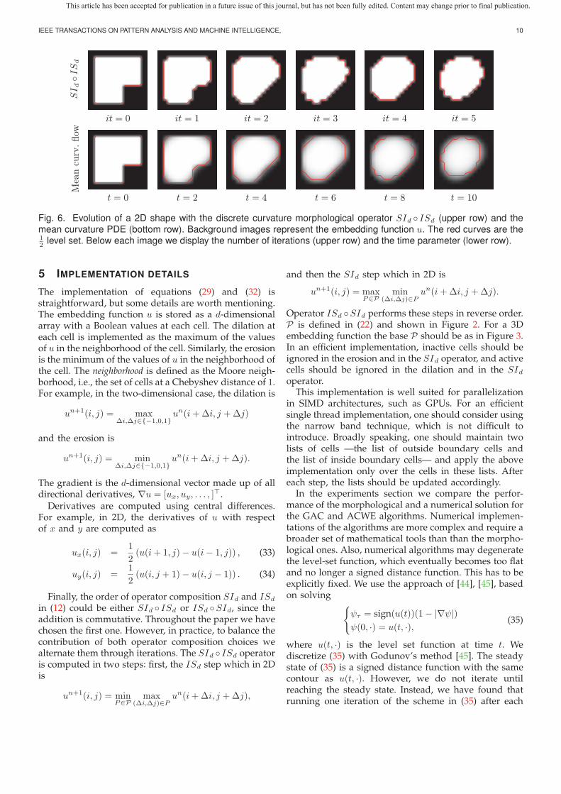
Fig. 6. Evolution of a 2D shape with the discrete curvature morphological operator SId ◦ ISd (upper row) and themean curvature PDE (bottom row). Background images represent the embedding function u. The red curves are the12 level set. Below each image we display the number of iterations (upper row) and the time parameter (lower row).

5 IMPLEMENTATION DETAILS

The implementation of equations (29) and (32) isstraightforward, but some details are worth mentioning.The embedding function u is stored as a d-dimensionalarray with a Boolean values at each cell. The dilation ateach cell is implemented as the maximum of the valuesof u in the neighborhood of the cell. Similarly, the erosionis the minimum of the values of u in the neighborhood ofthe cell. The neighborhood is defined as the Moore neigh-borhood, i.e., the set of cells at a Chebyshev distance of 1.For example, in the two-dimensional case, the dilation is

un+1(i, j) = maxΔi,Δj∈{−1,0,1}

un(i+Δi, j +Δj)

and the erosion is

un+1(i, j) = minΔi,Δj∈{−1,0,1}

un(i+Δi, j +Δj).

The gradient is the d-dimensional vector made up of alldirectional derivatives, ∇u = [ux, uy, . . . , ]

.Derivatives are computed using central differences.

For example, in 2D, the derivatives of u with respectof x and y are computed as

ux(i, j) =1

2(u(i+ 1, j)− u(i− 1, j)) , (33)

uy(i, j) =1

2(u(i, j + 1)− u(i, j − 1)) . (34)

Finally, the order of operator composition SId and ISd

in (12) could be either SId ◦ ISd or ISd ◦SId, since theaddition is commutative. Throughout the paper we havechosen the first one. However, in practice, to balance thecontribution of both operator composition choices wealternate them through iterations. The SId ◦ ISd operatoris computed in two steps: first, the ISd step which in 2Dis

un+1(i, j) = minP∈P

max(Δi,Δj)∈P

un(i+Δi, j +Δj),

and then the SId step which in 2D is

un+1(i, j) = maxP∈P

min(Δi,Δj)∈P

un(i+Δi, j +Δj).

Operator ISd ◦SId performs these steps in reverse order.P is defined in (22) and shown in Figure 2. For a 3Dembedding function the base P should be as in Figure 3.In an efficient implementation, inactive cells should beignored in the erosion and in the SId operator, and activecells should be ignored in the dilation and in the SIdoperator.

This implementation is well suited for parallelizationin SIMD architectures, such as GPUs. For an efficientsingle thread implementation, one should consider usingthe narrow band technique, which is not difficult tointroduce. Broadly speaking, one should maintain twolists of cells —the list of outside boundary cells andthe list of inside boundary cells— and apply the aboveimplementation only over the cells in these lists. Aftereach step, the lists should be updated accordingly.

In the experiments section we compare the perfor-mance of the morphological and a numerical solution forthe GAC and ACWE algorithms. Numerical implemen-tations of the algorithms are more complex and require abroader set of mathematical tools than than the morpho-logical ones. Also, numerical algorithms may degeneratethe level-set function, which eventually becomes too flatand no longer a signed distance function. This has to beexplicitly fixed. We use the approach of [44], [45], basedon solving {

ψτ = sign(u(t))(1− |∇ψ|)

ψ(0, ·) = u(t, ·),(35)

where u(t, ·) is the level set function at time t. Wediscretize (35) with Godunov’s method [45]. The steadystate of (35) is a signed distance function with the samecontour as u(t, ·). However, we do not iterate untilreaching the steady state. Instead, we have found thatrunning one iteration of the scheme in (35) after each



iteration of the scheme for the numerical solution sufficesto prevent the degeneration of the level-set function. Thisis the approach used in our experiments.

As in the morphological implementation, we discretizethe level set function u using a two-dimensional array.Here, each cell stores a floating point value. We use thecentral differences scheme for the spatial discretizationof the PDEs. The grid spacing is fixed to 1, so thefirst derivatives are given by (33) and (34). The secondderivatives are

uxx(i, j) = u(i+ 1, j) + u(i− 1, j)− 2u(i, j),

uyy(i, j) = u(i, j + 1) + u(i, j − 1)− 2u(i, j),

uxy(i, j) =1

4(u(i+ 1, j + 1)− u(i− 1, j + 1)

−u(i+ 1, j − 1) + u(i− 1, j − 1)).

The curvature is discretized as

div(∇u

‖∇u‖

)=

uxxu2y − 2uxyuxuy + uyyu

2x(

u2x + u2

y

) 32

.

The other terms in PDEs (26) and (31) are straight-forward to compute using the first and second orderderivatives.

The discretization of the time is done with the forward(explicit) method. The time step Δt is dynamically deter-mined so that the CFL condition is met but the evolutionis not too slow.

6 EXPERIMENTAL RESULTS

Besides its theoretical relevance, the morphologicalframework introduced in this work also presents ad-vantages in terms of required computational resources,simplicity and stability. The aim of the experimentsconducted is comparing qualitatively and quantitativelythe performance of the morphological and numericalevolution algorithms.

6.1 Smoothing

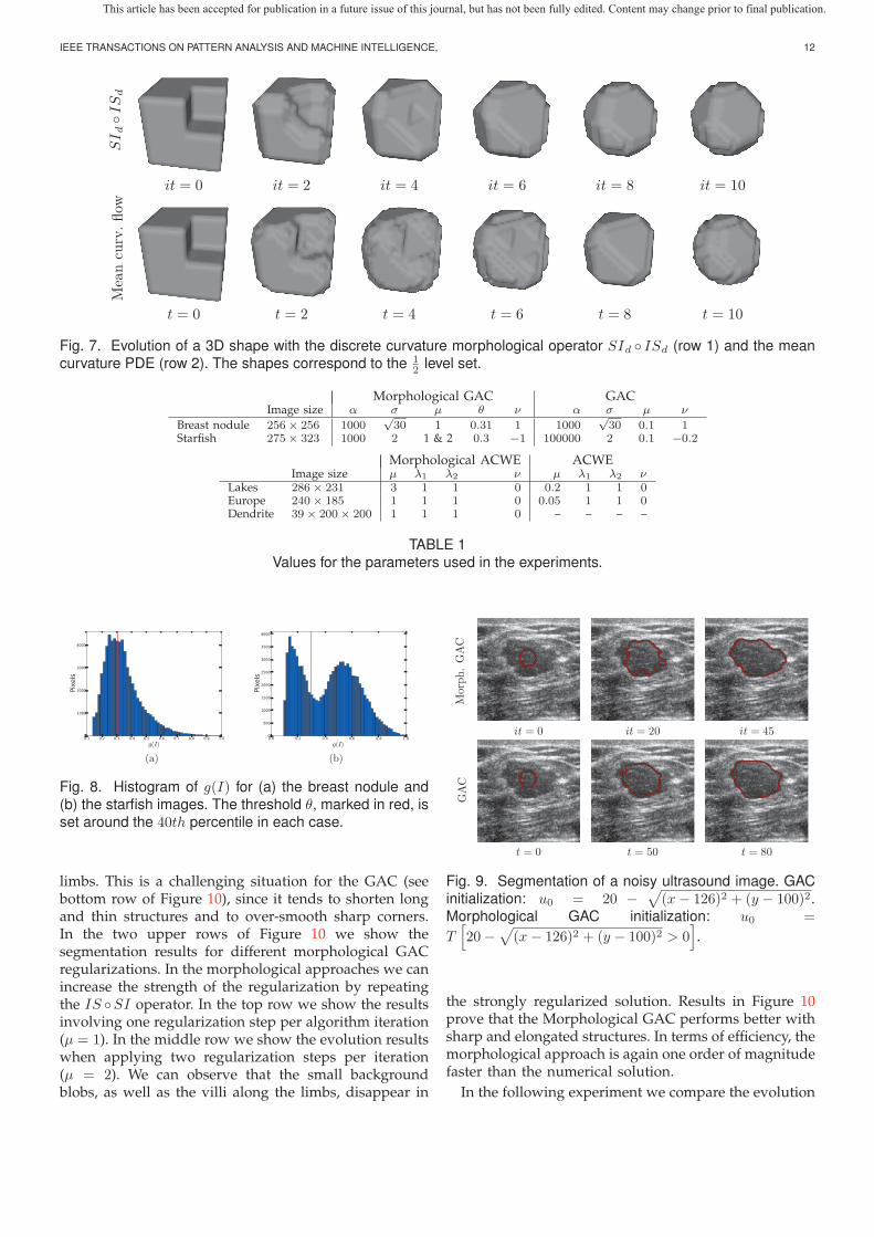
First, we qualitatively compare the smoothing achievedwith the discrete curvature morphological operator,SId ◦ ISd, and that obtained with the numerical solutionof the mean curvature PDE (2). Figures 6 and 7 compareboth methods in 2D and 3D respectively. The 2D caseshown in Figure 6 starts the evolution at a 13×13 pixelssquare with a corner of size 5 × 5 pixels removed. InFigure 7, the initial shape is a 16 × 16 × 16 pixels cubewith the 7× 7× 7 pixels corner removed. In the 2D (3D)experiments we can see that both the numerical and mor-phological approaches smooth the interface graduallytowards a circular (spherical) shape. In the 2D evolutioncase (see Figure 6) the curve at iteration number 5(last column) in the morphological algorithm is mostsimilar to the numerical mean curvature result for timet = 8. Something similar occurs for the 3D evolutionat iteration number 6 and time t = 8. In both cases itis not easy to decide which is the best pair of curves

to compare, since we do not have an analytic relationbetween parameter t of the numerical mean curvatureevolution and the number of iterations of the discretemorphological curvature approach. Nevertheless, thequalitative analysis of Figures 6 and 7 confirms that themorphological and numerical smoothing operators of 2Dand 3D interfaces is very similar.

6.2 Contour evolution

Our next group of experiments assess the performance ofthe morphological approaches of contour evolution andcompare their results with the numerical solution of theirassociated PDEs. We have implemented the GAC (26),ACWE (31), Morphological GAC (29) and MorphologicalACWE (32) models in C++ (only the 2D approaches) andPython (both 2D and 3D approaches). For comparisonpurposes, all implementations are single-threaded, andthey do not use improvement methods such as multi-scale or narrow-band solutions, although all approacheswould equally benefit from them. We run the experi-ments on a Intel Core 2 Duo 2.4 GHz. When given,evolution times always refer to those obtained with theC++ implementation.

Determining the parameters of the morphological al-gorithms is not a complex task. The MorphologicalGAC approach of (29) has parameters θ, ν and μ. Thesmoothing strength μ serves as a scaling value. When welook for small elements, μ should be small (i.e., 1) andlarge otherwise. The parameter θ —the threshold of theballoon and the smoothing— depends on g(I). A goodstarting point is to set θ as the 40th percentile of g(I)(see Figure 8). The stopping criterion g of (24) has twoparameters: α and σ. Parameter σ is assigned to matchthe size of the image borders. The algorithm is not verydependent on parameter α. A high value, such as 1000or 10000 should be enough in most cases.

The parameters of the Morphological ACWE are muchsimpler to set up and less sensitive to perturbations thanthe Morphological GAC. This approach does not requirea threshold θ. The balloon force is seldom necessary. Itworks directly on the image I . It does not use a stoppingcriterion g. For the experiments, we have set λ1 = λ2 = 1and ν = 0. The strength of the smoothing μ behaves as inthe morphological GAC. It should be low when we lookfor small elements and large otherwise. Table 1 summa-rizes the parameter values used in our experiments.

In Figures 9 and 10 we compare the performance of themorphological and the numerical GAC in challengingconditions. In Figure 9 we run both algorithms on anoisy ultrasound image of a breast nodule. Althoughthe final results are similar, the morphological method isalmost one order of magnitude faster than its numericalcounterpart (see Table 2). This experiment also confirmsthat the Morphological GAC works well in very noisyconditions.

The starfish image in Figure 10 has non-convex parts,elongated limbs and sharp angles at the junction of the



SId◦ISd

it = 0 it = 2 it = 4 it = 6 it = 8 it = 10

Meancu

rv.flow

t = 0 t = 2 t = 4 t = 6 t = 8 t = 10

Fig. 7. Evolution of a 3D shape with the discrete curvature morphological operator SId ◦ ISd (row 1) and the meancurvature PDE (row 2). The shapes correspond to the 1

2 level set.

Morphological GAC GACImage size α σ μ θ ν α σ μ ν

Breast nodule 256× 256 1000√30 1 0.31 1 1000

√30 0.1 1

Starfish 275× 323 1000 2 1 & 2 0.3 −1 100000 2 0.1 −0.2

Morphological ACWE ACWEImage size μ λ1 λ2 ν μ λ1 λ2 ν

Lakes 286× 231 3 1 1 0 0.2 1 1 0

Europe 240× 185 1 1 1 0 0.05 1 1 0

Dendrite 39× 200× 200 1 1 1 0 – – – –

TABLE 1Values for the parameters used in the experiments.

0.1 0.2 0.3 0.4 0.5 0.6 0.7 0.8 0.9 1.0

g(I)

0

1000

2000

3000

4000

Pixels

0.0 0.2 0.4 0.6 0.8 1.0

g(I)

0

500

1000

1500

2000

2500

3000

3500

4000

Pixels

(a) (b)

Fig. 8. Histogram of g(I) for (a) the breast nodule and(b) the starfish images. The threshold θ, marked in red, isset around the 40th percentile in each case.

limbs. This is a challenging situation for the GAC (seebottom row of Figure 10), since it tends to shorten longand thin structures and to over-smooth sharp corners.In the two upper rows of Figure 10 we show thesegmentation results for different morphological GACregularizations. In the morphological approaches we canincrease the strength of the regularization by repeatingthe IS ◦SI operator. In the top row we show the resultsinvolving one regularization step per algorithm iteration(μ = 1). In the middle row we show the evolution resultswhen applying two regularization steps per iteration(μ = 2). We can observe that the small backgroundblobs, as well as the villi along the limbs, disappear in

Morph.GAC

it = 0 it = 20 it = 45

GAC

t = 0 t = 50 t = 80

Fig. 9. Segmentation of a noisy ultrasound image. GACinitialization: u0 = 20 −

√(x− 126)2 + (y − 100)2.

Morphological GAC initialization: u0 =

T[20−

√(x− 126)2 + (y − 100)2 > 0

].

the strongly regularized solution. Results in Figure 10prove that the Morphological GAC performs better withsharp and elongated structures. In terms of efficiency, themorphological approach is again one order of magnitudefaster than the numerical solution.

In the following experiment we compare the evolution



of the energies in the morphological and numericalGAC. Since the parameters in the starfish example aredifferent for the Morphological GAC and the standardGAC (note that α = 103 in the first case and α = 106

in the second one) their energies are not comparable. Inorder to perform a comparison between the evolutionof the energies for both methods, we ran again theGAC algorithm with α = 103. Figure 11(a) shows theevolution of the energy of the Morphological GAC (i.e.,the evolution seen in Figure 10) and the energy of theGAC with the new parameter set. The energy for themorphological version of the algorithm is computedwith the parameter μ = 0.1 given in Table 1 for theircontinuous counterparts, since the parameter μ = 2 ofthe morphological methods is meaningless for energycomputation. Note that in both cases the global trendin the evolution tends to decrease the energy. How-ever, in both approaches, it increases in some intervalsalong the evolution. This is due to both the balloonforce term included in the PDE, that is not part of theminimized energy, and the fact that functional gradientdescent optimization does not guarantees that the energyalways decreases. Note also that the evolution of theenergy for the GAC continues to fall below the minimumenergy reached by its morphological counterpart. Thisis because the borders of the starfish limbs are almostperpendicular to the front of evolution and they are notcapable of stopping the shrinkage of the curve. Hence, itcontinues to evolve until it becomes a point and thereforeits energy is zero. It is a well-known problem of the GACmodel that the global minimum of the energy is reachedwhen the curve shrinks to a point. Therefore, the imagesegmentation with GAC heavily relies on the existenceof local minima.

In Figures 12 and 13 we compare the performanceof the morphological and numerical ACWE. In the firstFigure we segment a group of lakes in a satellite im-age. Here both methods work in uninformative (zero-gradient) areas without the balloon force. Also, the initialcurve u0 does not require to surround the objects. Wealso consider the detection of point clouds in images,where the ACWE model is known to work much betterthan the GAC [10]. Figure 13 depicts the evolution of acurve guided by an image of Europe night lights. Again,morphological and numerical results are very similar,with the morphological algorithm outperforming thenumerical one in terms of processing time (see Table 2).The evolution of the energy for the ACWE-based

methods in the lakes experiment is plotted in Fig-ure 11(b). As above, the parameter μ for computing theenergy of the morphological ACWE is the continuousone μ = 0.2. The morphological parameter μ = 3 ismeaningless for energy computation. We observe that inthe case of ACWE the energies of both methods have nooscillations and steadily decrease in each iteration. Thisnice behavior is due to the fact that the ACWE energy isexpected to be smoother than the GAC one because ofthe area global terms and the lack of the balloon force

Morph.GAC

(μ=

1)

it = 0 it = 80 it = 110

Morph.GAC

(μ=

2)

it = 0 it = 80 it = 110

GAC

t = 0 t = 4000 t = 5000

Fig. 10. Segmentation of elongated and narrowstructures. GAC initialization u0 = 135 −√(x− 138)2 + 3

4 (y − 163)2. Morphological GAC initializa-

tion u0 = T[135−

√(x− 138)2 + 3

4 (y − 163)2 > 0].

0 20 40 60 80 100 120

Iteration

250

300

350

400

450

500

550

Energy

0 100 200 300 400 500 600 700Time

0 50 100 150 200

Iteration

800

1000

1200

1400

1600

1800

2000

2200

2400

Energy

0 200 400 600 800 1000 1200 1400Time

(a) (b)

Fig. 11. Evolution of the energy of (a) the Morphologi-cal GAC and the continuous GAC in the starfish experi-ment and (b) the Morphological ACWE and the continu-ous ACWE in the lakes experiment. The blue continuousline plots the energy versus the number of iterations forthe morphological methods. The green dashed line plotsthe energy versus the time for the continuous methods.

present in the GACmodel. Moreover, they both convergeto nearly the same energy value.

We also validate our model with a 3D image stackfrom the area of neuroscience. In this experiment we canevaluate the morphological evolution of a surface in 3Dspace. We use a section of cortex tissue captured witha confocal microscopy corresponding to the 3D imageof a dendrite. A small 2-sphere is manually placed inthe center of the image. Then, the 3D MorphologicalACWE evolves the surface according to the contents ofthe image. Some steps of the evolution are depicted inFigure 14(a). The final results are shown in Figure 14(b).

Finally, we also make a quantitative comparison ofthe evolution achieved by the algorithms that we are



Morph.ACW

E

it = 0 it = 100 it = 180

ACW

E

t = 0 t = 800 t = 1400

Fig. 12. Lakes segmentation. ACWE initialization u0 =20 −

√(x− 170)2 + (y − 80)2. Morphological ACWE ini-

tialization u0 = T[20−

√(x− 170)2 + (y − 80)2 > 0

].

Morph.ACW

E

it = 0 it = 50 it = 130

ACW

E

t = 0 t = 1800 t = 3200

Fig. 13. Europe night-lights. ACWE initialization u0 =115−max{|x− 120|, 1.3 · |y − 92|}. Morphological ACWEu0 = T [115−max{|x− 120|, 1.3 · |y − 92|} > 0].

evaluating. We use the Jaccard similarity coefficient toquantify the comparison. Let u and v be two differentcontours, and χu and χv be the set of cells inside thecontours, i.e., the set of cells such that u(x) > 0 andv(x) > 0. The Jaccard similarity between u and v is

J(u, v) =|χu ∩ χv|

|χu ∪ χv|. (36)

It has value 1 when u and v are equal and 0 whenthey do not share any cell. Table 2 shows the similaritiesfor the pairs of contours obtained in each experiment.They are high (around 0.9) in most cases. In the starfishexperiment, however, the similarity is lower (0.64). Aninspection of Figure 10 reveals that the morphologicalGAC fits more accurately the image while the numericalapproach loses details at the ends of the arms and in thejunctions.

6.3 Morphological turbopixels

Many computer vision algorithms work with percep-tually meaningful entities of the image, obtained froma low-level grouping of pixels, called superpixels [19],[46]. Here we introduce the morphological turbopixels al-gorithm, as an example of an intrinsically local contour

it = 0 it = 20

it = 60 it = 160(a)

(b)

Fig. 14. Dendrite image stack. (a) Evolutionof 3D Morphological ACWE. The initialization isu0 = T

[10−

√(x− 20)2 + (y − 100)2 + (z − 100)2 > 0

].

(c) Final result.

evolution application that provides a set of compact andregular superpixels.

Turbopixels [19] compute a dense oversegmentationof an image by growing curves from many seeds dis-tributed throughout the image domain via a geometricflow similar to the Geodesic Active Contours. Curvesemanating from different seeds are not allowed to mergeinto a single curve. To meet this constraint, a homo-topy preserving thinning is carried out, which gives theskeleton of the area outside the curves, and partition theimage domain into one cell for each curve. The curvesare then confined to grow within their cell.

We have adapted the turbopixels to work with ourmorphological GAC, leading to the morphological tur-bopixels (see Algorithm 1). The homotopic thinning ap-proach that we use in the steps 5 and 8 of Algorithm 1 isa type of skeletonization that preserves the topology. Tothis end, we use a variation of the flux-ordered thinningalgorithm [47] that ignores the condition of being an end-point. The homotopic thinning computes a mask whichconfines each curve in its own cell, as shown in Figure 15.After several iterations, these cells will eventually be the



Morphological methods Continuous methodsExperiment Processing time Iterations Processing time Iterations Speedup J

Breast nodule 0.79s 45 6.85s 268 8.67 0.87Starfish (μ = 1) 2.46s 110 28.17s 864 11.45 0.64

Lakes 5.61s 180 21.90s 867 3.9 0.95Europe 1.18s 130 17.10s 989 14.5 0.91

TABLE 2Running times and number of iterations of the morphological methods vs. the continuous PDEs. Last columns showthe speedup gained by the morphological methods and the Jaccard similarity of the results between both methods.

superpixels. The morphological GAC with a mask be-haves essentially like the standard morphological GAC,but it does not allow that the evolving curves go into themasked areas. Thus we avoid that curves growing fromdifferent seeds merge. The extension from morphologicalturbopixels to morphological turbovoxels, i.e., the three-dimensional counterpart, is trivial.

Algorithm 1 Morphological turbopixelsInput: The separation among consecutive seeds s, num-

ber of iterations n and image I1: Place seeds on a rectangular grid with step s2: Perturb the seeds away from I high gradient regions

3: u ← binary level set with 1 in seeds locations and0 everywhere else

4: for i ∈ {0, . . . , n− 1} do5: B ← homotopic_thinning(u)6: u← One iteration of morphological GAC of uwith

mask B and stopping criterion g(I)7: end for8: B ← homotopic_thinning(u)

Output: The boundaries of the superpixels B

Figure 16 shows some results obtained with the mor-phological turbopixels in two images. The top imagebelongs to the Berkeley database and allows qualitativecomparison with the standard numerical implementa-tion in [19]. The bottom image diplays the results foran Electron Microscopy (EM) image of a pice of braintissue.

7 CONCLUSIONS

This paper introduces new results relating MathematicalMorphology and PDE approaches for image analysis.We have introduced a new curvature morphologicaloperator valid for surfaces of any dimension. On thebasis of this new operator we approximate the numericalsolution of surface evolution PDEs by the successivecomposition of morphological operators whose infinites-imal behavior is equivalent to the terms in the PDE.We have used this approach to provide morphologicalimplementations of the Geodesic Active Contour, the ActiveContours Without Borders and the Turbopixels algorithms.The morphological approach has several advantages

(a)

(b)

Fig. 15. (a) The level set function u describes multipleevolving curves. (b) Homotopic thinning gives a mask Bthat confines each curve within its own cell. The morpho-logical GAC with mask B will evolve the curves avoidingthat each curve passes through the walls of B.

over the numerical solution of the PDEs. The implemen-tation is simpler and has fewer parameters. There areno numerical instability issues and, since the level setfunction is binary and does not represent a distance, itrequires no re-initialization.

The experiments conducted confirm that the solutionsobtained with the morphological methods are compa-rable to those obtained with the numerical ones, withthe exception of narrow and elongated structures inwhich the morphological approach better fits the im-age. Morphological methods outperform their traditionalfunctional gradient descent numerical counterparts interms of stability and speed. In general, morphological



Fig. 16. Morphological turbopixels. (top) Image from theBerkeley Database; (bottom) EM image of brain tissue.

algorithms are about one order of magnitude faster,which makes them suitable for real-time applicationsin resource-limited hardware such as tracking in mo-bile devices, or for processing large images such asthose from EM imaging in neuroscience applications.Moreover, the morphological approach could also bene-fit from improvements devised to speed-up numericalalgorithms, such as the narrow band and multi-scaleimplementations.

ACKNOWLEDGMENTS

The authors would like to thank the anonymous re-viewers for their valuable comments and constructivesuggestions. This research was funded by the Cajal BlueBrain Project.

REFERENCES

[1] A. Blake and M. Isard, Active Contours. Springer, 1998. 1[2] M. Kass, A. Witkin, and D. Terzopoulos, “Snakes: Active contour

models,” International Journal of Computer Vision, vol. 1, no. 4, pp.321–331, 1988. 1

[3] O. Faugeras and R. Keriven, “Variational principles, surface evo-lution, pdes, level set methods, and the stereo problem,” IEEETransactions on Image Processing, vol. 7, no. 3, pp. 336–344, mar1998. 1

[4] N. Paragios and R. Deriche, “Geodesic active contours and levelsets for the detection and tracking of moving objects,” IEEETransactions on Pattern Analysis and Machine Intelligence, vol. 22,pp. 266–280, 2000. 1

[5] Y. Rathi, N. Vaswani, A. Tannenbaum, and A. Yezzi, “Trackingdeforming objects using particle filtering for geometric activecontours,” IEEE Transactions on Pattern Analysis and Machine In-telligence, vol. 29, no. 8, pp. 1470–1475, August 2007. 1

[6] A. Mishra, P. Fieguth, and D. Clausi, “Decoupled active contour(dac) for boundary detection,” IEEE Transactions on Pattern Anal-ysis and Machine Intelligence, vol. 33, no. 2, pp. 310–324, February2011. 1

[7] C. Zimmer and J. C. Olivo-Marin, “Coupled parametric activecontours,” IEEE Transactions on Pattern Analysis and Machine Intel-ligence, vol. 27, pp. 1838–1842, 2005. 1

[8] N. Paragios and R. Deriche, “Geodesic active regions and levelset methods for motion estimation and tracking,” Computer Visionand Image Understanding, vol. 97, no. 3, pp. 259 – 282, 2005. 1

[9] Y. Shi and W. C. Karl, “A real-time algorithm for the approxi-mation of level-set-based curve evolution,” IEEE Transactions onImage Processing, vol. 17, no. 5, pp. 645 –656, May 2008. 1, 2

[10] T. F. Chan and L. A. Vese, “Active contours without edges,” IEEETransactions on Image Processing, vol. 10, no. 2, pp. 266–277, 2001.1, 2, 7, 9, 13

[11] L. Vese and T. Chan, “A multiphase level set framework for imagesegmentation using the mumford and shah model,” InternationalJournal of Computer Vision, vol. 50, no. 3, pp. 271–293, December2002. 1

[12] B. Nilsson and A. Heyden, “A fast algorithm for level set-likeactive contours,” Pattern Recognition Letters, vol. 24, June 2003. 1,2

[13] D. Cremers, M. Rousson, and R. Deriche, “A review of statisticalapproaches to level set segmentation: integrating color, texture,motion and shape,” International Journal of Computer Vision, vol. 72,no. 2, pp. 195–215, April 2007. 1

[14] X.-F. Wang, D.-S. Huang, and H. Xu, “An efficient local chan-vese model for image segmentation,” Pattern Recognition, vol. 43,March 2010. 1

[15] C. Lenglet, J. Campbell, M. Descoteaux, G. Haro, P. Savadjiev,D. Wassermann, A. Anwander, R. Deriche, G. Pike, G. Sapiro,K. Siddiqi, and P. Thompson, “Mathematical methods for diffu-sion MRI processing,” Neuroimage, vol. 45, no. 1, pp. S111–S122,2009. 1

[16] C. Bibby and I. D. Reid, “Robust real-time visual tracking usingpixel-wise posteriors,” in Proc. European Conference on ComputerVision, 2008, pp. II: 831–844. 1, 2

[17] P. Chockalingam, N. Pradeep, and S. Birchfield, “Adaptivefragments-based tracking of non-rigid objects using level sets,” inProc. International Conference on Computer Vision, 2009, pp. 1530–1537. 1, 2

[18] D. Mitzel, E. Horbert, A. Ess, and B. Leibe, “Multi-person trackingwith sparse detection and continuous segmentation,” in Proc.European Conference on Computer Vision, 2010, pp. 397–410. 1

[19] A. Levinshtein, A. Stere, K. N. Kutulakos, D. J. Fleet, S. J.Dickinson, and K. Siddiqi, “Turbopixels: Fast superpixels usinggeometric flows,” IEEE Transactions on Pattern Analysis and Ma-chine Intelligence, vol. 31, no. 12, pp. 2290–2297, December 2009.1, 2, 14, 15

[20] V. Caselles, R. Kimmel, and G. Sapiro, “Geodesic active contours,”International Journal of Computer Vision, vol. 22, no. 1, pp. 61–79,1997. 1, 2, 7

[21] S. Kichenassamy, A. Kumar, P. Olver, A. Tannenbaum, andA. Yezzi, “Gradient flows and geometric active contour models,”in Proc. International Conference on Computer Vision, June 1995, pp.810 –815. 1

[22] S. Osher and J. A. Sethian, “Fronts propagating with curvature-dependent speed: algorithms based on hamilton-jacobi formula-tions,” J. Comput. Phys., vol. 79, no. 1, pp. 12–49, 1988. 1, 3

[23] S. Osher and R. Fedkiw, Level Set Methods and Dynamic ImplicitSurfaces. Springer, 2003. 1

[24] J. Weickert, B. M. T. H. Romeny, and M. A. Viergever, “Efficientand reliable schemes for nonlinear diffusion filtering,” IEEE Trans-actions on Image Processing, vol. 7, pp. 398–410, 1998. 1

[25] R. Goldenberg, R. Kimmel, E. Rivlin, and M. Rudzsky, “Fastgeodesic active contours,” IEEE Transactions on Image Processing,vol. 10, no. 10, pp. 1467–1475, 2001. 1, 2

[26] R. Tsai and S. Osher, “Level set methods and their applicationsin image science,” Comm. Math Sci, vol. 1, no. 4, pp. 1–20, 2003. 1

[27] G. Barles and P. E. Souganidis, “A New Approach to Front Prop-agation Problems: Theory and Applications,” Archive for Rational



Mechanics and Analysis, vol. 141, no. 3, pp. 237–296, March 1998.1

[28] Y. Shi and W. C. Karl, “Real-time tracking using level sets,”in Proceedings of the 2005 IEEE Computer Society Conference onComputer Vision and Pattern Recognition, vol. 2, 2005, pp. 34–41.2

[29] Y. Pan, B. JD, and S. Djouadi, “Efficient implementation of theChan-Vese models without solving PDEs,” in 2006 IEEE 8thWorkshop on Multimedia Signal Processing, October 2006, pp. 350–354. 2

[30] L. D. Cohen and R. Kimmel, “Global minimum for active con-tour models: A minimal path approach,” International Journal ofComputer Vision, vol. 24, no. 1, pp. 57–78, August 1997. 2

[31] B. Appleton and H. Talbot, “Globally optimal geodesic activecontours,” Journal of Mathematical Imaging and Vision, vol. 23, no. 1,pp. 67–86, July 2005. 2

[32] X. Bresson, S. Esedoglu, P. Vandergheynst, J.-P. Thiran, andS. Osher, “Fast global minimization of the active contour/snakemodel,” Journal of Mathematical Imaging and Vision, vol. 28, no. 2,pp. 151–167, June 2007. 2

[33] T. Pock, T. Schoenemann, G. Graber, H. Bischof, and D. Cremers,“A convex formulation of continuous multi-label problems,” inProc. European Conference on Computer Vision, 2008, pp. 792–805. 2

[34] T. Pock, D. Cremers, H. Bischof, and A. Chambolle, “An algorithmfor minimizing the mumford-shah functional.” in Proc. Interna-tional Conference on Computer Vision, 2009, pp. 1133–1140. 2

[35] J. Morales, L. Alonso-Nanclares, J. R. Rodriguez, J. Defelipe,A. Rodriguez, and A. Merchan-Perez, “Espina: a tool for theautomated segmentation and counting of synapses in large stacksof electron microscopy images,” Frontiers in Neuroanatomy, vol. 5,no. 18, 2011. 2

[36] P. Lax, “Numerical solution of partial differential equations,”Math. Monthly, vol. 72, pp. 74–85, 1965. 2

[37] L. Alvarez, F. Guichard, P.-L. Lions, and J.-M. Morel, “Axiomsand fundamental equations of image processing,” Arch. RationalMech. Anal., vol. 16, pp. 200–257, 1993. 2, 4

[38] R. van den Boomgaard and A. Smeulders, “The morphologicalstructure of images: The differential equations of morphologicalscale-space,” IEEE Transactions on Pattern Analysis and MachineIntelligence, vol. 16, no. 11, pp. 1101–1113, November 1994. 2

[39] R. Kimmel, Numerical Geometry of Images: Theory, Algorithms, andApplications. Springer Verlag, 2003. 2, 3

[40] F. Guichard, J. Morel, and R. Ryan, Contrast invariantimage analysis and PDE’s, 2004. [Online]. Available:http://mw.cmla.ens-cachan.fr/~morel/JMMBookOct04.pdf 2, 3,5

[41] F. Catté, F. Dibos, and G. Koepfler, “A morphological scheme formean curvature motion and applications to anisotropic diffusionand motion of level sets,” SIAM Journal on Numerical Analysis,vol. 32, no. 6, pp. 1895–1909, 1995. 2, 3, 4, 5

[42] L. Alvarez, L. Baumela, P. Henríquez, and P. Márquez-Neila,“Morphological snakes,” in Proc. International Conference on Com-puter Vision and Pattern Recognition, 2010, pp. 2197 – 2202. 2

[43] L. D. Cohen, “On active contour models and balloons,” CVGIP:Image Understanding, vol. 53, no. 2, pp. 211–218, 1991. 8

[44] M. Sussman, P. Smereka, and S. Osher, “A level set approachfor computing solutions to incompressible two-phase flow,” J.Comput. Phys., vol. 114, pp. 146–159, September 1994. 10

[45] S. Chen, B. Merriman, S. Osher, and P. Smereka, “A simple levelset method for solving Stefan problems,” J. Comput. Phys., vol.135, pp. 8–29, July 1997. 10

[46] X. Ren and J. Malik, “Learning a classification model for segmen-tation,” in Proc. International Conference on Computer Vision, vol. 1,2003, pp. 10–17. 14

[47] K. Siddiqi, S. Bouix, A. Tannenbaum, and S. W. Zucker,“Hamilton-jacobi skeletons,” International Journal of Computer Vi-sion, vol. 48, no. 3, pp. 215–231, July 2002. 14

Pablo Márquez-Neila received a BS in Com-puter Science from the Universidad de Ex-tremadura in 2006 and a MS in Artificial In-telligence from the Universidad Politécnica deMadrid (UPM) in 2008, where he is currentlycompleting his PhD. He has been member of theComputer Perception Group of the UPM since2008. His research interests lie in theoreticaland applied computer vision and related fieldsin computer graphics. He has worked in medi-cal imaging analysis and visualization, graphical

models for image processing and segmentation, and image registration.

Luis Baumela BS and MS, 1989, PhD, 1995,all in Computer Science from the UniversidadPolitécnica de Madrid. From 1989 to 1992 hewas an engineer at Telefónica’s R&D labs. Since1997 he is Associate Professor of Computer Sci-ence at the Facultad de Informática of the Uni-versidad Politécnica de Madrid where he leadsthe Computer Perception Group. His researchinterests include image alignment, face imageanalysis and medical imaging.

Luis Alvarez has received a M.Sc.in appliedmathematics in 1985 and a Ph.D. in mathe-matics in 1988, both from Complutense Uni-versity (Madrid, Spain). Between 1991 and1992 he worked as post-doctoral researcherat CEREMADE laboratory in the computer vi-sion research group directed by Prof. Jean-Michel Morel. Since 2000 he is full professor atthe University of Las Palmas de Gran Canaria(ULPGC). He has created the research groupAnálisis Matemático de Imágenes (AMI) at the

ULPGC. He is an expert in computer vision and applied mathematics.His main research interest areas are the applications of mathematicalanalysis to computer vision including problems like multiscale analysis,mathematical morphology, optic flow estimation, stereo vision, shaperepresentation, medical imaging, synthetic image generation, cameracalibration, etc.


Date post:	22-Apr-2018
Category:	Documents
Upload:	phamdung
View:	219 times
Download:	2 times

IEEE TRANSACTIONS ON PATTERN ANALYSIS AND MACHINE ... -...

Documents