IEEE TRANSACTIONS ON PATTERN ANALYSIS AND MACHINE INTELLIGENCE, VOL. XX, NO. Y, MONTH 2003 1 Layered Motion Segmentation and Depth Ordering by Tracking Edges Paul Smith, Tom Drummond Member, IEEE, and Roberto Cipolla Member, IEEE Abstract This paper presents a new Bayesian framework for motion segmentation—dividing a frame from an image sequence into layers representing different moving objects—by tracking edges between frames. Edges are found using the Canny edge detector, and the Expectation-Maximisation algorithm is then used to fit motion models to these edges and also to calculate the probabilities of the edges obeying each motion model. The edges are also used to segment the image into regions of similar colour. The most likely labelling for these regions is then calculated by using the edge probabilities, in association with a Markov Random Field-style prior. The identification of the relative depth ordering of the different motion layers is also determined, as an integral part of the process. An efficient implementation of this framework is presented for segmenting two motions (fore- ground and background) using two frames. It is then demonstrated how, by tracking the edges into further frames, the probabilities may be accumulated to provide an even more accurate and robust estimate, and segment an entire sequence. Further extensions are then presented to address the segmentation of more than two motions. Here, a hierarchical method of initialising the Expectation- Maximisation algorithm is described, and it is demonstrated that the Minimum Description Length principle may be used to automatically select the best number of motion layers. The results from over 30 sequences (demonstrating both two and three motions) are presented and discussed. Index Terms Video analysis, Motion, Segmentation, Depth cues Manuscript received November, 2000; revised March 2002; revised April 2003. The authors are with the Department of Engineering, University of Cambridge, Cambridge CB2 1PZ, UK. E-mail: {pas1001,twd20,cipolla}@eng.cam.ac.uk.
Transcript
IEEE TRANSACTIONS ON PATTERN ANALYSIS AND MACHINE INTELLIGENCE, VOL. XX, NO. Y, MONTH 2003 1
Layered Motion Segmentation and Depth
Ordering by Tracking Edges
Paul Smith, Tom DrummondMember, IEEE,
and Roberto CipollaMember, IEEE
Abstract
This paper presents a new Bayesian framework for motion segmentation—dividing a frame from
an image sequence into layers representing different moving objects—by tracking edges between
frames. Edges are found using the Canny edge detector, and the Expectation-Maximisation algorithm
is then used to fit motion models to these edges and also to calculate the probabilities of the edges
obeying each motion model. The edges are also used to segment the image into regions of similar
colour. The most likely labelling for these regions is then calculated by using the edge probabilities,
in association with a Markov Random Field-style prior. The identification of the relative depth
ordering of the different motion layers is also determined, as an integral part of the process.
An efficient implementation of this framework is presented for segmenting two motions (fore-
ground and background) using two frames. It is then demonstrated how, by tracking the edges into
further frames, the probabilities may be accumulated to provide an even more accurate and robust
estimate, and segment an entire sequence. Further extensions are then presented to address the
segmentation of more than two motions. Here, a hierarchical method of initialising the Expectation-
Maximisation algorithm is described, and it is demonstrated that the Minimum Description Length
principle may be used to automatically select the best number of motion layers. The results from
over 30 sequences (demonstrating both two and three motions) are presented and discussed.
Index Terms
Video analysis, Motion, Segmentation, Depth cues
Manuscript received November, 2000; revised March 2002; revised April 2003.
The authors are with the Department of Engineering, University of Cambridge, Cambridge CB2 1PZ, UK. E-mail:
{pas1001,twd20,cipolla}@eng.cam.ac.uk.
2 IEEE TRANSACTIONS ON PATTERN ANALYSIS AND MACHINE INTELLIGENCE, VOL. XX, NO. Y, MONTH 2003
I. I NTRODUCTION
Motion is an important cue in vision, and the analysis of the motion between two images,
or across a video sequence, is a prelude to many further areas in computer vision. Where there
are different moving objects in the scene, or objects at different depths, motion discontinuities
will occur and these provide information essential to the understanding of the scene. Motion
segmentation (the division of a video frame into areas obeying different image motions)
provides this valuable information.
With the current boom in digital media, motion segmentation finds itself a number of direct
applications. Video compression becomes increasingly important as consumers demand higher
quality for less bandwidth, and here motion segmentation can provide assistance. By detecting
and separating the moving objects from the background, coding techniques can apply different
coding strategies to the different elements of the scene. Typically, the background changes
less quickly, or is less relevant than the foreground action, so can be coded at a lower bit
rate. Mosaicing of the background [1], [2] provides another compact representation. The
MPEG-4 standard [3] explicitly describes a sequence in terms of objects moving in front
of a background image and, while initially designed for multimedia presentations, motion
segmentation may be used to also encode real video in this manner.
Another relatively new field is that of video indexing [4], [5], where the aim is to auto-
matically classify and retrieve video sequences based on their content. The segmentation of
the moving objects enables these objects and the background to be analysed independently.
Classification, both on low-level image and motion characteristics of the scene components,
and on higher-level semantic analysis can then take place.
A. Review of Previous Work
Many popular approaches to motion segmentation revolve around analysing the per-pixel
optic flow in the image. Optic flow techniques, such as the classic work by Horn and Schunk
[6], use spatiotemporal derivatives of the pixel intensities to provide a motion vector at each
pixel. Because of the aperture problem, this motion vector can only be determined in the
direction of the local intensity gradient, and so in order to determine the complete field it is
assumed that the motion is locally smooth.
Analysing this optic flow field is one approach to motion segmentation. Adiv [7] clustered
together pixels with similar flow vectors and then grouped these into segments obeying
the same 3D motion; Murray and Buxton [8] followed a similar technique. However, the
SMITH, DRUMMOND AND CIPOLLA: MOTION SEGMENTATION BY TRACKING EDGES 3
smoothing required by optic flow algorithms renders the flow fields highly unreliable both
in areas of low gradient (into which results from other areas spread), and when there are
multiple motions. The case of multiple motions is particularly troublesome, since the edges
of moving objects create discontinuities in the flow field, and after smoothing the localisation
of these edges is difficult. It is unfortunate that these are the very edges that are required for
a motion segmentation. One solution to this smoothing problem is to apply the smoothing
in a piecewise fashion. Taking a small area, the flow can be analysed to determine whether
it best fits one smooth motion or a pair of motions, and these patches in the image can be
marked and treated accordingly (e.g. [9], [10], [11]).
The most successful approaches to motion segmentation consider parameterising the optic
flow field, fitting a different model (typically 2D affine) to each moving object. Pixels can then
be labelled as best fitting one model or another. This is referred to as alayered representation
[10] of the motion field, since it models pixel motions as belonging to one of several layers.
Each layer has its own, smooth, flow field, while discontinuities can occur between layers.
Each layer represents a different object in the sequence, and so the assignment of pixels to
layers also provides the motion segmentation.
There are two main approaches to determining the contents of the layers, of which the
dominant motionapproach (e.g. [1], [12], [13], [14], [15]) is the most straightforward. Here,
a single motion is robustly fitted to all pixels, which are then tested to see whether they
really fit that motion (according to some metric). The pixels which agree with the motion are
labelled as being on that layer. At this stage, either this layer can be labelled as ‘background’
(being the dominant motion), and the outlier pixels as belonging to foreground objects [14],
[15], or the process can be repeated recursively on the remaining pixels to provide a full set
of layers for further analysis [1], [12], [13].
The other main approach is to determine all of the motions simultaneously. This can either
be done either by estimating a large number of motions, one for each small patch of the image,
and then merging similar motions (typically byk-means clustering) [10], [11], [16], or by
using the Expectation-Maximisation (EM) algorithm [17] to simultaneously estimate motions
and find the pixel labels [2], [18], [19]. The number of motions also has to be determined.
This is usually done by either setting a smoothing factor and merging convergent models [19],
or by considering the size of the model under a Minimum Description Length framework
[18].
Given a set of motions, assigning pixels to layers requires determining which motion they
4 IEEE TRANSACTIONS ON PATTERN ANALYSIS AND MACHINE INTELLIGENCE, VOL. XX, NO. Y, MONTH 2003
best fit, if any. This can be done by comparing the pixel colour or intensities under the
proposed motions, but this presents several problems. Pixels in areas of smooth intensity are
ambiguous as they can appear similar under several different motions and, as with the optic
flow techniques, some form of smoothing is required to identify the best motion for these
regions. Pixels in areas of high intensity gradient are also troublesome, as slight errors in the
motion estimate can yield pixel of a very different colour or intensity, even under the correct
motion. Again, some smoothing is usually required. A common approach is to use a Markov
Random field [20], which encourages pixels to be labelled the same as their neighbours [14],
[15], [19], [21]. This works well at ensuring coherent regions, but can often also lead to the
foreground objects ‘bleeding’ over their edge by a pixel or two.
All of the techniques considered so far try to solve the motion segmentation problem using
only motion information. This, however, ignores the wealth of additional information that is
present in the image intensity structure. The image structure and the pixel motion can both be
considered at the same time by assigning a combined score to each pixel and then finding the
optimal segmentation based on all these properties, as in Shi and Malik’s Normalized Cuts
framework [22], but these approaches tend to be computationally expensive. A more efficient
approach is that ofregion merging, where an image is first segmented solely according to the
image structure, and then objects are identified by merging regions with the same motion.
This implicitly resolves the problems identified earlier which required smoothing of the optic
flow field, since the static segmentation process will group together neighbouring pixels of
similar intensity so that all the pixels in an area of smooth intensity, being grouped in the
same region, will be labelled with the same motion. Regions will be delimited by areas
of high gradient (edges) in the image and it is at these points that changes in the motion
labelling may occur.
As with the per-pixel optic flow methods, the region-merging approach has several methods
of simultaneously finding the motions and labelling the regions. Under the dominant-motion
method (e.g. [4], [12], [23]), a single parametric motion is robustly fitted to all the pixels
and then regions which agree with this motion are segmented as one layer and the process
repeated on the rest. Alternatively, a different motion may be fitted to each region and then
some clustering performed in parameter space to group regions with similar motions [24],
[25], [26], [27], [28], [29]. The EM algorithm is also a good choice when faced with this
type of estimation problem [19].
The final segmentation from all of these motion segmentation schemes is a labelling of
SMITH, DRUMMOND AND CIPOLLA: MOTION SEGMENTATION BY TRACKING EDGES 5
pixels, each into one of several layers, together with the parameterised motion for each layer.
What is not generally considered is the relative depth ordering of each of these layers i.e.
which is the background and which are foreground objects. If necessary, it is sometimes
assumed that the largest region or the dominant motion is the background. Occlusion is
commonly considered, but only in terms of a problem which upsets the pixel matching and
so requires the use of robust methods. However, this occlusion may be used to identify the
layer ordering as a post-processing stage. Wang and Adelson [10], and Bergen and Meyer
[29], identify the occasions when a group of pixels on the edge of a layer are outliers to the
layer motion and use these to infer that the layer is being occluded by its neighbour. Tweed
and Calway [30] use similar occlusion reasoning around the boundaries of regions as part of
an integrated segmentation and ordering scheme.
Depth ordering has recently begun to be considered as an integral part of the segmentation
process. Black and Fleet [31] have modelled occlusion boundaries directly by considering
the optic flow in a small region and this also allows occluding edges to be detected and
the relative ordering to be found. Gaucher and Medioni [32] also study the velocity field to
detect motion boundaries and infer the occlusion relationships.
B. This Paper: Using Edges
This paper presents a novel and efficient framework for both motion segmentation and
depth ordering using the motion of edges in the sequence. Previous researchers have found
that that the motion of pixels in areas of smooth intensity is difficult to determine and that
smoothing is required to resolve this problem, although this then provides problems of its
own. This paper ignores these areas initially, concentrating only on edges, and then follows
a region-merging framework, labelling pre-segmented regions according to their motions. It
is shown that the motion of these regions may be determined solely from the motion of their
edges without needing to use the pixels in their smooth interior. A similar approach was used
by Thompson [24], who also used only the motion of the edges of regions in estimating their
motion. However, this is his only use of the edges, as a prelude to a standard region-merging
approach. This paper shows that edges provide further information and, in fact, the clustering
and labelling of the region edges provides all the information that can be known about the
assignment of regions and also the ordering of the different layers.
This paper describes the theory linking the motions of edges and regions, and then develops
a probabilistic framework which enables the most likely region labelling and layer ordering
6 IEEE TRANSACTIONS ON PATTERN ANALYSIS AND MACHINE INTELLIGENCE, VOL. XX, NO. Y, MONTH 2003
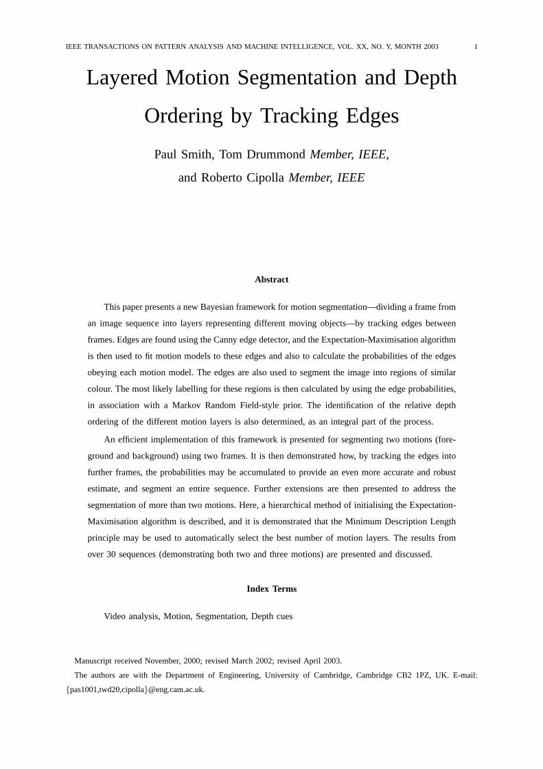
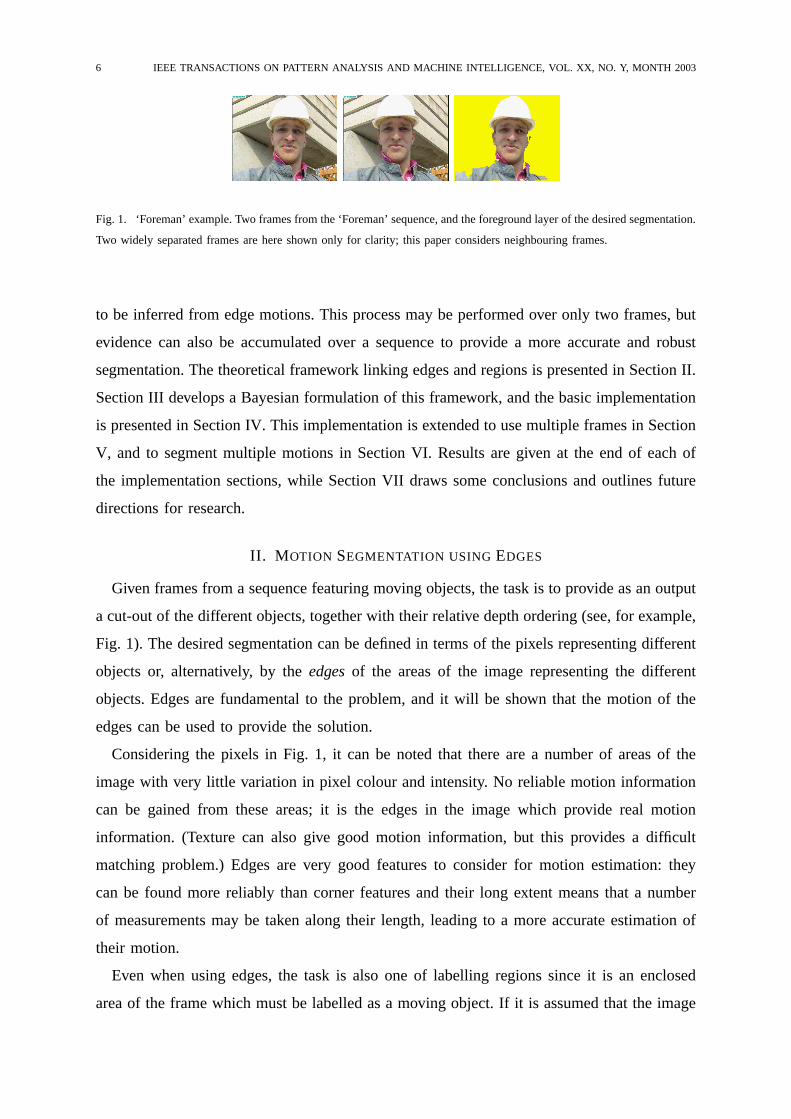
Fig. 1. ‘Foreman’ example. Two frames from the ‘Foreman’ sequence, and the foreground layer of the desired segmentation.
Two widely separated frames are here shown only for clarity; this paper considers neighbouring frames.
to be inferred from edge motions. This process may be performed over only two frames, but
evidence can also be accumulated over a sequence to provide a more accurate and robust
segmentation. The theoretical framework linking edges and regions is presented in Section II.
Section III develops a Bayesian formulation of this framework, and the basic implementation
is presented in Section IV. This implementation is extended to use multiple frames in Section
V, and to segment multiple motions in Section VI. Results are given at the end of each of
the implementation sections, while Section VII draws some conclusions and outlines future
directions for research.
II. M OTION SEGMENTATION USING EDGES
Given frames from a sequence featuring moving objects, the task is to provide as an output
a cut-out of the different objects, together with their relative depth ordering (see, for example,
Fig. 1). The desired segmentation can be defined in terms of the pixels representing different
objects or, alternatively, by theedgesof the areas of the image representing the different
objects. Edges are fundamental to the problem, and it will be shown that the motion of the
edges can be used to provide the solution.
Considering the pixels in Fig. 1, it can be noted that there are a number of areas of the
image with very little variation in pixel colour and intensity. No reliable motion information
can be gained from these areas; it is the edges in the image which provide real motion
information. (Texture can also give good motion information, but this provides a difficult
matching problem.) Edges are very good features to consider for motion estimation: they
can be found more reliably than corner features and their long extent means that a number
of measurements may be taken along their length, leading to a more accurate estimation of
their motion.
Even when using edges, the task is also one of labelling regions since it is an enclosed
area of the frame which must be labelled as a moving object. If it is assumed that the image
SMITH, DRUMMOND AND CIPOLLA: MOTION SEGMENTATION BY TRACKING EDGES 7
is segmented into regions along edges, then there is a natural link between the regions and
the edges.
A. The Theory of Edges and Regions
Edges in an image are generated as a result of the texture of objects, or their boundaries in
the scene.1 There are three fundamental assumptions made in this work, which are commonly
made in layered-motion schemes, and will be valid in many sequences:
1) As an object moves all of the edges associated with that object move, with a motion
which may be approximately described by some motion model.
2) The motions are layered, i.e. one motion takes place completely in front of another, and
the layers are strictly ordered. Typically the layer farthest from the camera is referred
to as the background, with nearer foreground layers in front of this.
3) No one segmented image region belongs to two or more motion models, and hence any
occluding boundary is visible as an region edge in the image.
Given these assumptions it is possible to state the relationship between the motions of regions
and the motions of the edges that divide them. If the layer of each region is known, and
the layer ordering is known, then the layer of each edge can be uniquely determined by the
following rule:
Edge Labelling Rule:The layer to which an edge belongs is that of the nearer
of the two regions which it bounds.
The converse is not true. If only the edge labelling is known (and not the layer ordering),
then this does not necessarily determine the region labelling or layer ordering. Indeed, even
if the layer ordering is known, there may be multiple region labellings which are consistent
with the edge labelling.
An example of a region and edge labelling is shown in Fig. 2(a). On the left is shown a
known region labelling, where the dark circle is the foreground object. Since it is on top, all
of its edges are visible and move with the foreground motion, labelled as black in the edge
label image on the right. All of the edges of the grey background regions, except those that
also bound the foreground region, move with the background motion and so are labelled as
grey. The edge labelling is thus uniquely determined.
1Edges may also be generated as a result of material or surface properties (texture or reflectance). It is assumed that
these do not occur, but see the ‘Car’ sequence in Section IV for an example of the consequence of this assumption.
8 IEEE TRANSACTIONS ON PATTERN ANALYSIS AND MACHINE INTELLIGENCE, VOL. XX, NO. Y, MONTH 2003
(a) Region labelling Edge labelling (b)
BA
Motion 2
Motion 1
C
Fig. 2. Edges and Regions. (a) A region labelling and layer ordering (in this case black is on top) fully defines the edge
labelling. The edge labelling can also give the region labelling; (b) T-junctions (where edges of different motion labellings
meet) can be used to determine the layer ordering (see text).
If, instead, the edge labelling is known (but not the layer ordering), it is still possible
to make deductions about both the region labelling and the layer ordering. Regions which
are bounded by edges of different motions must be on a layer at least as far away as the
furthest of its bounding edges (if it were nearer, its edges would occlude edges at that layer).
However, for each edge, at least one of the regions that it divides must have the same layer
as the edge. A region labelling can be produced from an edge labelling, but ambiguities may
still be present—specifically, a single region in the middle of a foreground object may be a
hole through to the background, although this is unlikely.
A complete segmentation also requires the layer ordering to be determined and, importantly,
this can usually be determined from the edge labelling. Fig. 2(b) highlights a T-junction from
the previous example, where edges with two different labellings meet. To determine which
of the two motion layers is on top, both of the two possibilities are hypothesised and tested.
Regions A and B are bounded by edges of two different motions, which can only occur
when these regions are bounded by edges obeying their own motion and also an edge of
the occluding object. These regions therefore must belong to the relative ‘background’. The
question is: which of the the two motions is the background motion? If it is hypothesised
that the background motion is motion 2 (black), then these regions should be labelled as
obeying motion 2, and the edge between them should also obey motion 2. However, it is
already known that the edge between them obeys motion 1, so this cannot be the correct layer
ordering. If motion 1 were background and motion 2 foreground then the region labelling
would be consistent with the edge labelling, indicating that this is the correct layer ordering.
Fig. 3 shows an ambiguous case. Here, there are no T-junctions and so the layer ordering
cannot be determined. There are two possible interpretations, both consistent with the edge
labelling. Cases such as these are ambiguous under any motion segmentation scheme, and at
least the system presented here is able to identify such ambiguities.
SMITH, DRUMMOND AND CIPOLLA: MOTION SEGMENTATION BY TRACKING EDGES 9
Case 1 Case 2
Fig. 3. Ambiguous edges and regions. If there is no interaction between the edges of the two objects, there are two
possible interpretations of the central edge labelling. Either of the two motions could be foreground, resulting in slightly
different region labelling solutions. In case 1, the black circle is the foreground object; in case 2 it is on the background
(viewed through a rectangular window).
This section has shown that edges are not only a necessary element in an accurate motion
segmentation, they are also sufficient. Edges can be detected in a frame, labelled with their
motion, and then used to label the regions in between. In real images it is not possible to
determine an exact edge labelling, and so instead the next section develops a probabilistic
framework for performing this edge and region labelling.
III. B AYESIAN FORMULATION
There are a large number of parameters which must be solved to give a complete motion
segmentation and for which the most likely values must be estimated. Given that the task is
one of labelling the regions of a static segmentation, finding their motion, and determining
the layer ordering, the complete model of the segmentationM consists of the elements
M = {Θ,F ,R}, where
Θ is the parameters of the motion models,
F is the foreground-background ordering of the motion layers,
R is the motion label (layer) for each region.
The region edge labels are not an independent part of the model, but are completely defined
by R andF from the Edge Labelling Rule of Section II.
Given the image dataD (and any other prior information assumed about the world), the
task is to find the modelM with the maximum probability given this data and priors:
arg maxM
P (M |D) = arg maxRFΘ
P (RFΘ|D) (1)
This can be further decomposed, without any loss of generality, into a motion estimation
component and region labelling:
arg maxRFΘ
P (RFΘ|D) = arg maxRFΘ
P (Θ|D) P (RF |ΘD) (2)
10 IEEE TRANSACTIONS ON PATTERN ANALYSIS AND MACHINE INTELLIGENCE, VOL. XX, NO. Y, MONTH 2003
At this stage a simplification is made: it is assumed that the motion parametersΘ can
be maximised independently of the others i.e. the correct motions can be estimated without
knowing the region labelling (just from the edges). This relies on the richness of edges avail-
able in a typical frame, and the redundancy this provides. This motion estimate approaches
the global maximum but, if desired, a global optimisation may be performed once an initial
set of motions and region labelling has been found; this is discussed in Section VI. Given
this simplifying assumption, the expression to be maximised is:
arg maxΘ
P (Θ|D)
︸ ︷︷ ︸a
arg maxRF
P (RF |ΘD)
︸ ︷︷ ︸b
(3)
where the value ofΘ used in term (b) is that which maximises term (a). The two components
of (3) can be evaluated in turn: first (a), the motions, and then (b), the region labelling and
layer ordering.
A. Estimating the MotionsΘ
The first term in (3) estimates the motions between frames (Θ encapsulates the parameters
of all the motions). Thus far this statistical framework has not specified how the most likely
motion is estimated and neither are edges included. As explained in Section II, edges are
robust features to track, and they provide a natural link to the regions which are to be labelled.
The labelling of edges must be introduced into the statistical model: they are expressed by
the random variablee which gives, for each edge, the probability of it obeying each motion.
This is a necessary variable, since in order to estimate the motion models from the edges it
must be known which edges belong to which motion. However, simultaneously labelling the
edges and fitting motions is a circular problem, which may be resolved by expressing the
estimation ofΘ ande in terms of the Expectation-Maximisation algorithm [17], withe as
the hidden variable. This is expressed by the following equation:
arg maxΘn+1
∑e
log P (eD|Θn+1) P (e|ΘnD) (4)
This iterates between two stages: the E-stage computes the expectation, which forms the bulk
of this expression (the main computation work here is in calculating the edge probabilities
P (e|ΘnD)); the M-stage then maximises this expression, performing the maximisation of
(4) over Θn+1. Some suitable initialisation is used and then the two stages are iterated to
convergence, which has the effect of maximising (3a). An implementation of this is outlined
in Section IV.
SMITH, DRUMMOND AND CIPOLLA: MOTION SEGMENTATION BY TRACKING EDGES 11
B. Estimating the LabellingsR and F .
Having obtained the most likely motions, the remaining parameters of the modelM can
be maximised. These are the region labellingR and the layer orderingF , which provide
the final segmentation. Once again, the edge labels are used as an intermediate step. Given
the motionsΘ, the edge label probabilitiesP (e|ΘD) can be estimated, and from Section II
the relationship between edges and regions is known. Term (3b) is augmented by the edge
labelling e, which must then be marginalised, giving
arg maxRF
P (RF |ΘD) = arg maxRF
∑e
P (RF |eΘD) P (e|ΘD) (5)
= arg maxRF
∑e
P (RF |e) P (e|ΘD) (6)
where the first expression in (5) can be simplified sincee encapsulates all of the information
from Θ andD that is relevant to determining the final segmentationR andF , as shown in
Section II.
The second term, the edge probabilities, can extracted directly from the motion estimation
stage—it is used in the EM algorithm. The first term is more difficult to estimate, and it is
easier to recast this using Bayes’ Rule, giving
P (RF |e) =P (e|RF ) P (RF )
P (e)(7)
The maximisation is overR andF , soP (e) is constant. The prior probabilities ofR andF
are independent, since whether a particular layer is called ‘motion 1’ or ‘motion 2’ does not
change its labelling. Any foreground motion is equally likely, soP (F ) is constant, but the last
term,P (R), is not constant. This term is used to encode likely labelling configurations since
some configurations of region labels are more likely than others.2 This leaves the following
expression to be evaluated:
arg maxRF
∑e
P (e|RF ) P (R) P (e|ΘD) (8)
The P (e|RF ) term is very useful. The edge labellinge is only an intermediate variable,
and is entirely defined by the region labellingR and the foreground motionF . This prob-
ability therefore takes on a binary value—it is 1 if that edge labelling is implied and 0 if
2For example, individual holes in a foreground object are unlikely. This prior enables the ambiguous regions mentioned
in Section II to be given their most likely labelling.
12 IEEE TRANSACTIONS ON PATTERN ANALYSIS AND MACHINE INTELLIGENCE, VOL. XX, NO. Y, MONTH 2003
it is not. The sum in (8) can thus be removed, and thee in the final term replaced by the
function e(R, F ), which provides the correct edge labels for given values ofR andF .
arg maxRF
P (e (R, F )|ΘD)︸ ︷︷ ︸a
P (R)︸ ︷︷ ︸b
(9)
The variableF takes only a discrete set of values (for example, in the case of two layers,
only two: either one motion is foreground, or the other). Equation (9) can therefore be
maximised in two stages:F can be fixed at one value and the expression maximised overR,
and the process then repeated with other values ofF and the global maximum taken.3 The
maximisation overR can be performed by hypothesising a complete region labelling and
then testing the evidence (9a)—determining the implied edge labels and then calculating
the probability of the edge labelling given the motions—and the prior (9b), calculating
the likelihood of that particular labelling configuration. An exhaustive search is impractical
and, in the implementation presented in Section IV, region labellings are hypothesised using
simulated annealing. Maximising this expression is identical to maximising (3b), and is the
last stage of the motion segmentation algorithm: the most likelyR andF represent the most
likely region labelling and layer ordering.
IV. I MPLEMENTATION FOR TWO MOTIONS, TWO FRAMES
The Bayesian framework presented in Section III leads to an efficient implementation.
This section describes how a video frame may be divided into two layers (foreground and
background) using the information from one more frame. This is a common case and also the
simplest motion segmentation situation. Many of the details in this two motion, two frame
case apply to more general cases, which are mostly simple extensions. Sections V and VI
cover the multiple-frame and multiple-motion cases respectively.
The system progresses in two stages, as demonstrated in Fig. 4. The first is to detect edges,
find motions and label the edges according to their probability of obeying each motion. These
edge labels are sufficient to label the rest of the image. In the second stage the frame is divided
into regions of similar colour using these edges, and the motion labelling for these regions
which best agrees with the edge labelling is then determined.
3This stage is combinatorial in the number of layers. This presents difficulties for sequences with many layers, but there
are many real sequences with a small number of motions (for example, 36 sequences are considered in this work, all with
two or three layers).
SMITH, DRUMMOND AND CIPOLLA: MOTION SEGMENTATION BY TRACKING EDGES 13
(a) (b) (c) (d)
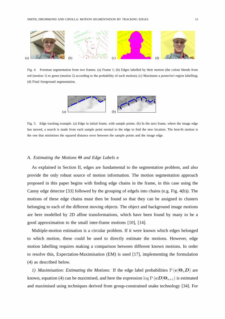
Fig. 4. Foreman segmentation from two frames. (a) Frame 1; (b) Edges labelled by their motion (the colour blends from
red (motion 1) to green (motion 2) according to the probability of each motion); (c) Maximuma posterioriregion labelling;
(d) Final foreground segmentation.
(a) (b)
Fig. 5. Edge tracking example. (a) Edge in initial frame, with sample points. (b) In the next frame, where the image edge
has moved, a search is made from each sample point normal to the edge to find the new location. The best-fit motion is
the one that minimises the squared distance error between the sample points and the image edge.
A. Estimating the MotionsΘ and Edge Labelse
As explained in Section II, edges are fundamental to the segmentation problem, and also
provide the only robust source of motion information. The motion segmentation approach
proposed in this paper begins with finding edge chains in the frame, in this case using the
Canny edge detector [33] followed by the grouping of edgels into chains (e.g. Fig. 4(b)). The
motions of these edge chains must then be found so that they can be assigned to clusters
belonging to each of the different moving objects. The object and background image motions
are here modelled by 2D affine transformations, which have been found by many to be a
good approximation to the small inter-frame motions [10], [14].
Multiple-motion estimation is a circular problem. If it were known which edges belonged
to which motion, these could be used to directly estimate the motions. However, edge
motion labelling requires making a comparison between different known motions. In order
to resolve this, Expectation-Maximisation (EM) is used [17], implementing the formulation
(4) as described below.
1) Maximisation: Estimating the Motions:If the edge label probabilitiesP (e|ΘnD) are
known, equation (4) can be maximised, and here the expressionlog P (eD|Θn+1) is estimated
and maximised using techniques derived from group-constrained snake technology [34]. For
14 IEEE TRANSACTIONS ON PATTERN ANALYSIS AND MACHINE INTELLIGENCE, VOL. XX, NO. Y, MONTH 2003
each edge, sample points are assigned at regular intervals along the edge (see Fig. 5(a)). The
motion of these sample points are considered to be representative of the edge motion (there
are about1, 400 sample points in a typical frame). The sample points from the first frame
are mapped into the next (either in the same location or, in further iterations, according to
the current motion estimate), and a search is made for the true edge location. Because of
the aperture problem, the motion of edges can only be determined in a direction normal
to the edge, but this is useful as it restricts the search for a matching edge pixel to a fast
one-dimensional search along the edge normal.
To find a match, colour image gradients are estimated in both the original image and the
proposed new location using a5×5 convolution kernel in the red, green and blue components
of the image. The match score is taken to be the sum of squared differences over the three
colours, in both thex and y directions. The search is made over the pixels normal to the
sample point location in the new image, to a maximum distance of 20 pixels.4 The image
distancedk, between the original location and its best match in the next image, is measured
(see Fig. 5(b)). If the score is below a threshold, ‘no match’ is returned instead.
At each sample point the expected image motion due to a 2D affine motionθ can be
calculated. A convenient formulation uses the Lie algebra of image transformations [34].
According to this, transformations in the General Affine group GA(2) may be decomposed
into a linear sum of the following generator matrices:
G1 =[
0 0 10 0 00 0 0
]G2 =
[0 0 00 0 10 0 0
]G3 =
[0 −1 01 0 00 0 0
]
G4 =[
1 0 00 1 00 0 0
]G5 =
[1 0 00 −1 00 0 0
]G6 =
[0 1 01 0 00 0 0
](10)
These act on homogeneous image coordinates(x y 1
)T
, and are responsible for the
following six motion fields in the image:
L1 = ( 10 ) L2 = ( 0
1 ) L3 = ( −yx )
L4 = ( xy ) L5 = ( x−y ) L6 = ( y
x ) (11)
The task is to estimate the amount,αi of each of these deformation modes.
Since measurements can only be taken normal to the edge,αi may be estimated by
minimising the geometric distance between the measurementsdk and the projection of the
4Testing has revealed that the typical maximum image motion is of the order of 10 pixels, so this is a conservative choice.
An adaptive search interval, or a multi-resolution approach, would be appropriate in more extreme cases.
SMITH, DRUMMOND AND CIPOLLA: MOTION SEGMENTATION BY TRACKING EDGES 15
fields onto the unit edge normalnk, over all of the sample points on that edge, or set of
edges ∑
k
(dk −∑
jαj
(Lj
k · nk))2
(12)
which is the negative log probability oflog P (eD|Θn+1), from (4), given an independent
Gaussian statistical model. This expression may be minimised by using the singular value
decomposition to give a least squares fit. In practice re-weighted least squares [35] is used
to provide robustness to outliers, using the weight function
w(x) =1
1 + |x| (13)
(for a full description, see [36]). This corresponds to using a Laplacian (i.e. non-Gaussian)
model for the errors, and is chosen because it gives a good fit to the observed distribution
(see Fig. 6). Having found theαi, an image motionθ is then given by the same linear sum
of the generators:
θ = I + αiGi (14)
To implement the M-stage of the EM algorithm (4), equation (12) is also weighted by
P (e|ΘnD) and then minimised to obtain the parameters of each motionθn+1 in turn. These
are then combined to giveΘn+1.
2) Expectation: Calculating Edge Probabilities:The discrete probability distributionP (e|ΘD)
gives the probability of an edge fitting a particular motion from the set of motionsΘ =
{θ1, θ2}, and the E-stage of (4) involves estimating this. This can be done by considering
the sample points used for motion estimation (for example, in Fig. 5 the first edge location,
with zero residual errors, is far more likely than the second one). It may be assumed that the
residual errors from sample points are representative of the whole edge, and that these errors
are independent.5 The likelihood that the edge fits a given motion is thus the product of the
likelihood of a correct match at each sample point along the edge. GivenΘ, the sample points
are matched under each motion and each edge likelihood calculated. Normalising these gives
the probability of each motion.
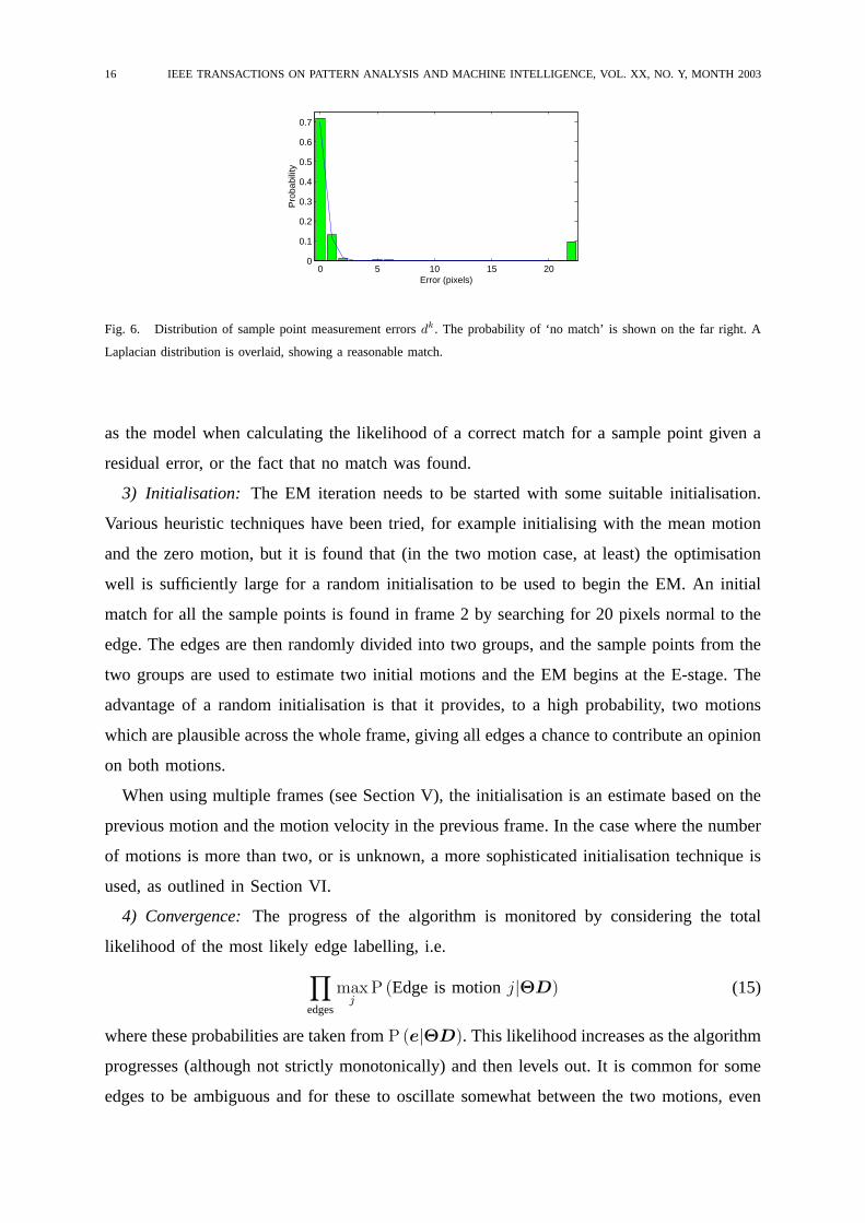
The distribution of sample point measurement errorsdk has been extracted from sample
sequences where the motion is known. The sample points are matched in their correct location
and their errors measured, giving the distribution shown in Fig. 6. This histogram is used
5This is not in fact the case, but making this assumption gives a much simpler solution while still yielding plausible
statistics. See [36] for a discussion of the validity of this assumption, and [37] for an alternative approach.
16 IEEE TRANSACTIONS ON PATTERN ANALYSIS AND MACHINE INTELLIGENCE, VOL. XX, NO. Y, MONTH 2003
0 5 10 15 200
0.1
0.2
0.3
0.4
0.5
0.6
0.7
Error (pixels)P
roba
bilit
y
Fig. 6. Distribution of sample point measurement errorsdk. The probability of ‘no match’ is shown on the far right. A
Laplacian distribution is overlaid, showing a reasonable match.
as the model when calculating the likelihood of a correct match for a sample point given a
residual error, or the fact that no match was found.
3) Initialisation: The EM iteration needs to be started with some suitable initialisation.
Various heuristic techniques have been tried, for example initialising with the mean motion
and the zero motion, but it is found that (in the two motion case, at least) the optimisation
well is sufficiently large for a random initialisation to be used to begin the EM. An initial
match for all the sample points is found in frame 2 by searching for 20 pixels normal to the
edge. The edges are then randomly divided into two groups, and the sample points from the
two groups are used to estimate two initial motions and the EM begins at the E-stage. The
advantage of a random initialisation is that it provides, to a high probability, two motions
which are plausible across the whole frame, giving all edges a chance to contribute an opinion
on both motions.
When using multiple frames (see Section V), the initialisation is an estimate based on the
previous motion and the motion velocity in the previous frame. In the case where the number
of motions is more than two, or is unknown, a more sophisticated initialisation technique is
used, as outlined in Section VI.
4) Convergence:The progress of the algorithm is monitored by considering the total
likelihood of the most likely edge labelling, i.e.
∏edges
maxj
P (Edge is motionj|ΘD) (15)
where these probabilities are taken fromP (e|ΘD). This likelihood increases as the algorithm
progresses (although not strictly monotonically) and then levels out. It is common for some
edges to be ambiguous and for these to oscillate somewhat between the two motions, even
SMITH, DRUMMOND AND CIPOLLA: MOTION SEGMENTATION BY TRACKING EDGES 17
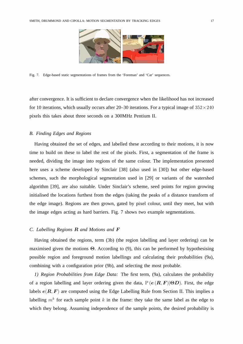
Fig. 7. Edge-based static segmentations of frames from the ‘Foreman’ and ‘Car’ sequences.
after convergence. It is sufficient to declare convergence when the likelihood has not increased
for 10 iterations, which usually occurs after 20–30 iterations. For a typical image of352×240
pixels this takes about three seconds on a 300MHz Pentium II.
B. Finding Edges and Regions
Having obtained the set of edges, and labelled these according to their motions, it is now
time to build on these to label the rest of the pixels. First, a segmentation of the frame is
needed, dividing the image into regions of the same colour. The implementation presented
here uses a scheme developed by Sinclair [38] (also used in [30]) but other edge-based
schemes, such the morphological segmentation used in [29] or variants of the watershed
algorithm [39], are also suitable. Under Sinclair’s scheme, seed points for region growing
initialised the locations furthest from the edges (taking the peaks of a distance transform of
the edge image). Regions are then grown, gated by pixel colour, until they meet, but with
the image edges acting as hard barriers. Fig. 7 shows two example segmentations.
C. Labelling RegionsR and Motions andF
Having obtained the regions, term (3b) (the region labelling and layer ordering) can be
maximised given the motionsΘ. According to (9), this can be performed by hypothesising
possible region and foreground motion labellings and calculating their probabilities (9a),
combining with a configuration prior (9b), and selecting the most probable.
1) Region Probabilities from Edge Data:The first term, (9a), calculates the probability
of a region labelling and layer ordering given the data,P (e (R,F )|ΘD). First, the edge
labelse(R,F ) are computed using the Edge Labelling Rule from Section II. This implies a
labelling mk for each sample pointk in the frame: they take the same label as the edge to
which they belong. Assuming independence of the sample points, the desired probability is
18 IEEE TRANSACTIONS ON PATTERN ANALYSIS AND MACHINE INTELLIGENCE, VOL. XX, NO. Y, MONTH 2003
then given by
P (e (R,F )|ΘD) =∏
k
P(mk|ΘD
)(16)
The probability of a particular motion labelling for each sample point,P(mk|ΘD
), was
calculated earlier in the E-stage of EM. The likelihood of the data is that from Fig. 6, and
is normalised according to Bayes’ rule (with equal priors) to give the motion probability.
2) Region Prior: Term (9b) encodes thea priori region labelling, reflecting the fact that
some arrangements of region labels are more likely than others. This is implemented using an
approach similar to a Markov Random Field (MRF) [20], where the probability of a region’s
labelling depends on its immediate neighbours. Given a region labellingR, a functionfr(R)
can be defined which is the proportion of the boundary which regionr shares with neighbours
of the same label. A long boundary with regions of the same label is more likely than very
little of the boundary bordering similar regions. A probability density function forfr has
been computed from hand-segmented examples, and can be approximated by
P (fr) =0.932
1 + exp (9− 18f)+ 0.034 0 < fr < 1 (17)
P (1) is set to 0.9992 andP (0) to 0.0008 to enforce the fact that isolated regions or holes
are particularly unlikely. The prior probability of a region labellingR is then given by
P (R) =∏
regionsr
P (fr(R))∑layersl=1 P (fr(R{r = l})) (18)
wherefr(R{r = l}) indicates the fractional boundary length which would be seen if the label
of regionr were substituted with a different labell.
3) Solution by Simulated Annealing:In order to maximise over all possible region la-
bellings, simulated annealing [40] is used. This begins with an initial guess at the region
labelling and then repeatedly tries flipping individual region labels one by one to see how
the change affects the overall probability. (This is a simple process since a single region label
change only causes local changes, and so (18) does not need completely re-evaluating.) The
annealing process is initialised with a guess based on the edge probabilities, and a reasonable
initialisation is to label the regions according to the majority of its edge labellings. The region
labels are taken in turn, considering the probability of the region being labelled motion 1 or
2 given its edge probabilities and the current motion label of its neighbours. At the beginning
of the annealing process, the region is then re-assigned a label by a Monte Carlo approach,
i.e. randomly according to the two probabilities. As the iterations progress, these probabilities
SMITH, DRUMMOND AND CIPOLLA: MOTION SEGMENTATION BY TRACKING EDGES 19
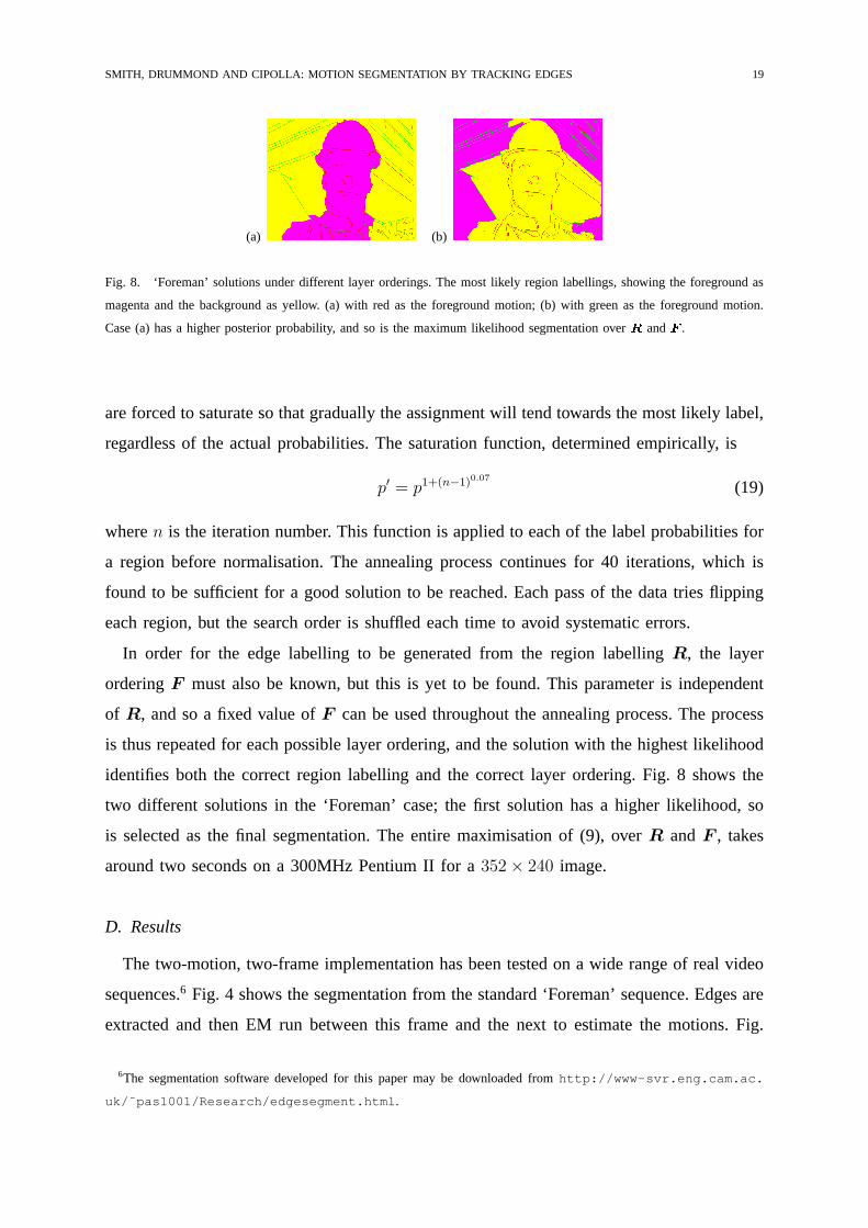
(a) (b)
Fig. 8. ‘Foreman’ solutions under different layer orderings. The most likely region labellings, showing the foreground as
magenta and the background as yellow. (a) with red as the foreground motion; (b) with green as the foreground motion.
Case (a) has a higher posterior probability, and so is the maximum likelihood segmentation overR andF .
are forced to saturate so that gradually the assignment will tend towards the most likely label,
regardless of the actual probabilities. The saturation function, determined empirically, is
p′ = p1+(n−1)0.07
(19)
wheren is the iteration number. This function is applied to each of the label probabilities for
a region before normalisation. The annealing process continues for 40 iterations, which is
found to be sufficient for a good solution to be reached. Each pass of the data tries flipping
each region, but the search order is shuffled each time to avoid systematic errors.
In order for the edge labelling to be generated from the region labellingR, the layer
orderingF must also be known, but this is yet to be found. This parameter is independent
of R, and so a fixed value ofF can be used throughout the annealing process. The process
is thus repeated for each possible layer ordering, and the solution with the highest likelihood
identifies both the correct region labelling and the correct layer ordering. Fig. 8 shows the
two different solutions in the ‘Foreman’ case; the first solution has a higher likelihood, so
is selected as the final segmentation. The entire maximisation of (9), overR and F , takes
around two seconds on a 300MHz Pentium II for a352× 240 image.
D. Results
The two-motion, two-frame implementation has been tested on a wide range of real video
sequences.6 Fig. 4 shows the segmentation from the standard ‘Foreman’ sequence. Edges are
extracted and then EM run between this frame and the next to estimate the motions. Fig.
6The segmentation software developed for this paper may be downloaded fromhttp://www-svr.eng.cam.ac.
uk/˜pas1001/Research/edgesegment.html .
20 IEEE TRANSACTIONS ON PATTERN ANALYSIS AND MACHINE INTELLIGENCE, VOL. XX, NO. Y, MONTH 2003
(a) (b) (c) (d)
Fig. 9. ‘Car’ segmentation from two frames. (a) Original frame; (b) Edge labels after EM; (c) Most likely region labelling;
(d) Final foreground segmentation.
4(b) shows the edges labelled according to how well they fit each motion after convergence.
It can be seen that this process labels most of the edges correctly, even though the motion is
small (about two pixels). The edges on his shoulders are poorly-labelled, but this is due to the
shoulders’ motion being even smaller than that of the head. The correct motion is selected
as foreground with very high confidence (> 99%) and the final segmentation, Fig. 4(d), is
excellent despite some poor edge labels. In this case the MRF region prior is a great help
in producing a plausible segmentation. Compared with the hand-picked segmentation shown
in Fig. 1(c), 98% of the regions are labelled correctly. On a 300MHz Pentium II, it takes a
total of around eight seconds to produce the motion segmentation (the image is352 × 288
pixels).
Fig. 9 shows the results from the ‘Car’ sequence, recorded for this work. Here the car
moves to the left, and is tracked by the camera. This is a rather unusual sequence since
more pixels belong to the foreground than to the background, and some dominant-motion
techniques may therefore assume the incorrect layer ordering. In this paper, however, the
ordering is found from the edge labels and no such assumption is made. Unfortunately, the
motion of many of the horizontal edges is ambiguous and also, with few T-junctions, there is
less depth ordering information than in the previous cases. Nevertheless, the correct motion
is identified as foreground, although with less certainty than in the previous cases. The final
segmentation (Fig. 9(d)) labels 96.2% of all pixels correctly (compared with a hand labelling),
and there are two main sources of error. As already noted, with both motions being horizontal,
the labelling of the horizontal edges is ambiguous. More serious, however, are the reflections
on the bonnet and roof of the car which naturally move with the background motion. The
edges are correctly labelled—as background—but this gives the incorrect semantic labelling.
Without higher-level processing (a prior model of a car), this problem is difficult to resolve.
One pleasing element of the solution is that the view through the car window has been
SMITH, DRUMMOND AND CIPOLLA: MOTION SEGMENTATION BY TRACKING EDGES 21
Fig. 10. A sample of the 34 test sequences, and their segmentations.
correctly segmented as background.
This implementation has been tested on a total of 34 real sequences. Full results can be
seen in [36], but Fig. 10 shows a selection of these further results. Compared with a manual
labelling of regions, a third of all the sequences tested are segmented near perfectly by the
system (> 95% of pixels correct), and a further third are good or very good (> 75%). In
the cases where the segmentation fails, this is either because the motion between frames is
extremely non-affine, or is ambiguous, resulting in a poor edge labelling.
For the algorithm to succeed the edges merely have to fitbetterunder one motion than the
other—an exact match is not necessary. As a result, even when one or both of the motions
are significantly non-affine, as in the first two examples in Fig. 10, a good segmentation
can still be generated. It is a testament to the sufficiency of edges that where the edges are
labelled correctly, the segmentation is invariably good. The principal way to improve a poor
edge labelling is to continue to track the edges over additional frames until the two motions
can be better distinguished.
V. EXTENSION TO MULTIPLE FRAMES
Accumulating evidence over a number of frames can resolve ambiguities that may be
present between the first two frames, and also makes the labelling more robust. This section
first describes how evidence can be accumulated over frames to improve the segmentation
of one frame, and then outlines how the techniques can be extended to segment a whole
sequence.
A. Accumulating Evidence to Improve Segmentations
While the segmentation of frame 1 using a pair of frames is often very good, a simple
extension allows this to be improved. The two-frame algorithm of Section IV can be run
22 IEEE TRANSACTIONS ON PATTERN ANALYSIS AND MACHINE INTELLIGENCE, VOL. XX, NO. Y, MONTH 2003
between frame 1 and other frames in the sequence to gather more evidence about the
segmentation of frame 1. The efficiency of this process can be improved by using the results
from one frame to initialise the next and, in particular, the EM stage can be given a better
initialisation. The initial motion estimate is that for the previous frame incremented by the
velocity between the previous two frames. The edge labelling is initialised to be that implied
by the region labelling of the previous frame, and the EM begins at the M-stage.
1) Combining statistics:The probability that an edge obeys a particular motion over a
sequence is the probability that it obeyed that motion between each of the frames. This
can be calculated from the product of the probabilities for that edge over all those frames,
if it is assumed that the image data yielding information about the labelling of each edge
is independent in each frame. The EM is performed only on the edge probabilities and the
motion between the frame in question and frame 1, but after convergence the final probabilities
are multiplied together with the probabilities from the previous frames to give the cumulative
edge statistics. The region and foreground labelling is then performed as described in Section
IV, but using the cumulative edge statistics.
2) Occlusion: The problem of occlusion was ignored when considering only two frames
since the effects are minimal, but occlusion becomes a significant problem when tracking
over multiple frames. Knowing the foreground/background labelling for edges and regions
in frame 1, and the motions between frames, enables this to be overcome. For each edge
labelled as background, its sample points are projected into frame 2 under the background
motion and are then projected back into frame 1 according to the foreground motion. If a
sample point falls into a region currently labelled as foreground, this foreground region must
move on top of that point in frame 2. If this is the case, the sample point is marked as
occluded and does not contribute to the tracking of its edge into frame 3. All sample points
are also tested to see if they project outside the frame under their motions and if so they are
also ignored. This process can be repeated for as many frames as is necessary.
B. Results
The success of the multiple frame approach can be seen in Fig. 11, showing the ‘Foreman’
example. Accumulating the edge probabilities over several frames allows random errors to
be removed and edge probabilities to be reinforced. The larger motions between more widely
separated frames also removes ambiguity. It can be seen that over time the consensus among
many edges on the shoulders is towards the foreground motion, and the accumulated edge
SMITH, DRUMMOND AND CIPOLLA: MOTION SEGMENTATION BY TRACKING EDGES 23
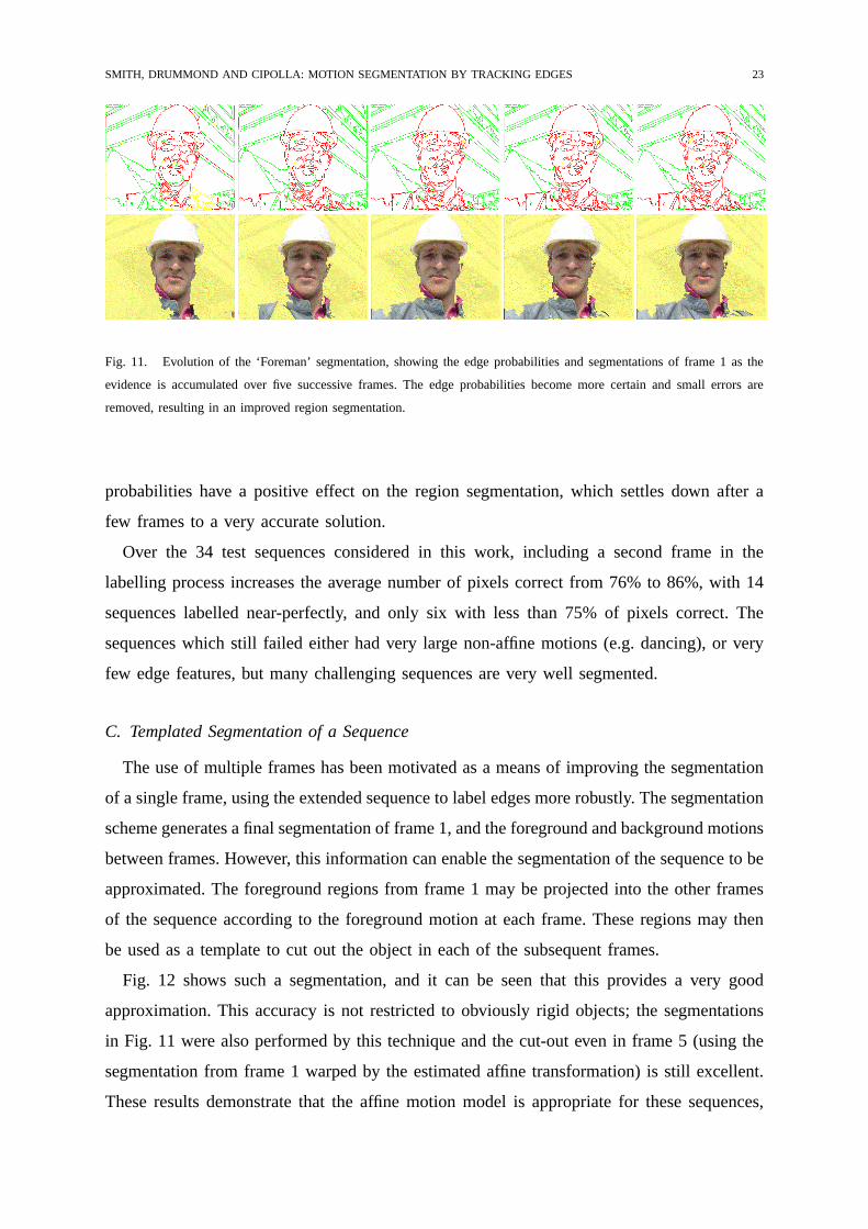
Fig. 11. Evolution of the ‘Foreman’ segmentation, showing the edge probabilities and segmentations of frame 1 as the
evidence is accumulated over five successive frames. The edge probabilities become more certain and small errors are
removed, resulting in an improved region segmentation.
probabilities have a positive effect on the region segmentation, which settles down after a
few frames to a very accurate solution.
Over the 34 test sequences considered in this work, including a second frame in the
labelling process increases the average number of pixels correct from 76% to 86%, with 14
sequences labelled near-perfectly, and only six with less than 75% of pixels correct. The
sequences which still failed either had very large non-affine motions (e.g. dancing), or very
few edge features, but many challenging sequences are very well segmented.
C. Templated Segmentation of a Sequence
The use of multiple frames has been motivated as a means of improving the segmentation
of a single frame, using the extended sequence to label edges more robustly. The segmentation
scheme generates a final segmentation of frame 1, and the foreground and background motions
between frames. However, this information can enable the segmentation of the sequence to be
approximated. The foreground regions from frame 1 may be projected into the other frames
of the sequence according to the foreground motion at each frame. These regions may then
be used as a template to cut out the object in each of the subsequent frames.
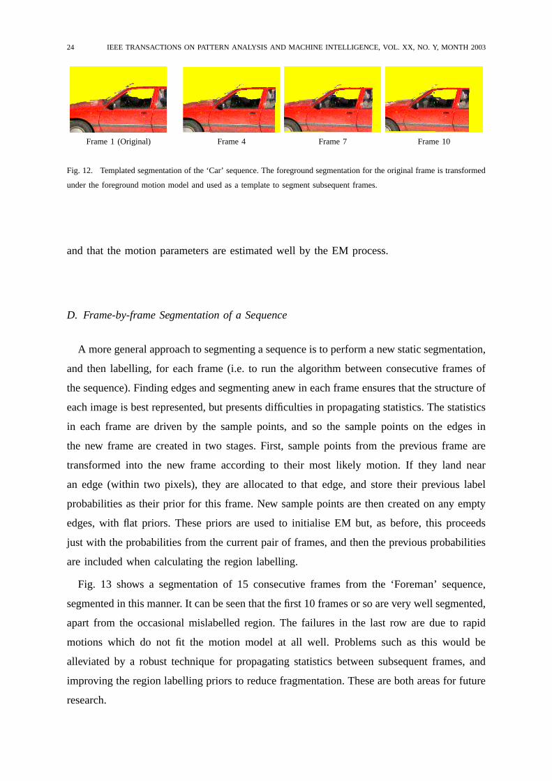
Fig. 12 shows such a segmentation, and it can be seen that this provides a very good
approximation. This accuracy is not restricted to obviously rigid objects; the segmentations
in Fig. 11 were also performed by this technique and the cut-out even in frame 5 (using the
segmentation from frame 1 warped by the estimated affine transformation) is still excellent.
These results demonstrate that the affine motion model is appropriate for these sequences,
24 IEEE TRANSACTIONS ON PATTERN ANALYSIS AND MACHINE INTELLIGENCE, VOL. XX, NO. Y, MONTH 2003
Frame 1 (Original) Frame 4 Frame 7 Frame 10
Fig. 12. Templated segmentation of the ‘Car’ sequence. The foreground segmentation for the original frame is transformed
under the foreground motion model and used as a template to segment subsequent frames.
and that the motion parameters are estimated well by the EM process.
D. Frame-by-frame Segmentation of a Sequence
A more general approach to segmenting a sequence is to perform a new static segmentation,
and then labelling, for each frame (i.e. to run the algorithm between consecutive frames of
the sequence). Finding edges and segmenting anew in each frame ensures that the structure of
each image is best represented, but presents difficulties in propagating statistics. The statistics
in each frame are driven by the sample points, and so the sample points on the edges in
the new frame are created in two stages. First, sample points from the previous frame are
transformed into the new frame according to their most likely motion. If they land near
an edge (within two pixels), they are allocated to that edge, and store their previous label
probabilities as their prior for this frame. New sample points are then created on any empty
edges, with flat priors. These priors are used to initialise EM but, as before, this proceeds
just with the probabilities from the current pair of frames, and then the previous probabilities
are included when calculating the region labelling.
Fig. 13 shows a segmentation of 15 consecutive frames from the ‘Foreman’ sequence,
segmented in this manner. It can be seen that the first 10 frames or so are very well segmented,
apart from the occasional mislabelled region. The failures in the last row are due to rapid
motions which do not fit the motion model at all well. Problems such as this would be
alleviated by a robust technique for propagating statistics between subsequent frames, and
improving the region labelling priors to reduce fragmentation. These are both areas for future
research.
SMITH, DRUMMOND AND CIPOLLA: MOTION SEGMENTATION BY TRACKING EDGES 25
Fig. 13. Segmentation of the ‘Foreman’ sequence. Segmentation of ten consecutive frames.
VI. EXTENSION TO MULTIPLE MOTIONS
The theory of Section III applies to any number of motions, and the implementation has
been developed so as to be extensible to more than two motions. Tracking and separating
three or more motions, however, is a non-trivial task. With more motions for edges to belong
to, there is less information with which to estimate each motion, and edges can be assigned
to a particular model with less certainty. In estimating the edge labels, the EM stage is found
to have a large number of local minima, and so an accurate initialisation is particularly
important. The layer ordering is also more difficult to establish. As the number of motions
increase, the number of possible layer hypotheses increases factorially. Also, with fewer
regions per motion, fewer regions interact with those of another layer, leading to fewer T-
junctions, which are the essential ingredient in determining the layer ordering. These factors
all contribute to the difficulty of the multiple motion case, and this section proposes some
extensions which make the problem easier.
A. EM Initialisation
The EM algorithm is guaranteed to converge to a maximum, but there is no guarantee
that this will be the global maximum. The most important element in EM is always the
initialisation and, for more than two motions, the EM algorithm will get trapped in a local
26 IEEE TRANSACTIONS ON PATTERN ANALYSIS AND MACHINE INTELLIGENCE, VOL. XX, NO. Y, MONTH 2003
maximum unless started with a good solution. The best solution to these local maxima
problems in EM remains an open question.
The approach adopted in this paper is hierarchical—the gross arrangement is estimated by
fitting a small number of models and then these are split to see if any finer detail can be
fitted. The one case where local minima does not present a significant problem is when there
are only two motions, where it has been found that any reasonable initialisation can be used.
Therefore, two motions are fitted first and then three-motion initialisations are considered near
to this solution. It is worth considering what happens in the case of labelling a three-motion
scene with only two motions. There are two likely outcomes:
1) One (or both) of the models adjusts to absorb edges which belong to the third motion.
2) The edges belonging to the third motion are discarded as outliers.
This provides a principled method for generating a set of three-motion initialisations. First
fit two motions, then:
1) Take the set of edges which best fit one motion and try to fit two motions to these by
splitting the edges into two random groups and performing EM on just these edges to
optimise the split. The original motion is then replaced with these two. Each of the two
initial motions can be split in this way, providing two different initialisations.
2) A third initialisation is given from the outliers by calculating the motion of the outlier
edges and adding it to the list of motions. Outlier edges are detected by comparing the
likelihood under the ‘correct motion’ statistics of Section IV with the likelihood under
an ‘incorrect motion’ model, also gathered from example data.
From each of these three initialisations, EM is run to find the most likely edge labelling
and motions. The likelihood of each solution is given by the product of the edge likelihoods
(under their most likely motion), and best solution is the one with the highest likelihood.
This solution may then be split further into more motions in the same manner.
B. Determining the Best Number of Motions
This hierarchical approach can also be used to identify the best number of motions to fit.
Increasing the number of models is guaranteed to improve the fit to the data and increase
the likelihood of the solution, but this must be balanced against the cost of using a large
number of motions. This is addressed by applying the Minimum Description Length (MDL)
principle, one of many model selection methods available [41]. This considers the cost of
SMITH, DRUMMOND AND CIPOLLA: MOTION SEGMENTATION BY TRACKING EDGES 27
encoding the observations in terms of the model and any residual error. A large number of
models or a large residual both give rise to a high cost.
The cost of encoding the model consists of two parts. Firstly, the parameters of the model:
each number is assumed to be encoded to 10-bit precision, and with six parameters per
model (2D affine), the cost is60nm (for nm models). Secondly, each edge must be labelled
as belonging to one of the models, which costslog2 nm for each of thene edges. The edge
residuals must also be encoded, and the cost for an optimal coding is equal to the total
negative logarithm (to base two) of the edge likelihoods,Le, giving
C = 60nm + ne log2 nm +∑
e
log2 Le (20)
The costC is be evaluated after each attempted initialisation, and the smallest cost indicates
the best solution and the best number of models.
C. Global Optimisation: Expectation-Maximisation-Constrain (EMC)
The region labelling is determined via two independent optimisations which use edges as an
intermediate representation: first the best edge labelling is determined, and then the best region
labelling given these edges. It has thus far been assumed that this is a good approximation
to the global optimum, but unfortunately this is not always the case, particularly with more
than two motions.
In the first EM stage the edges are assigned purely on the basis of how well they fit each
motion, with no consideration given to how likely that edge labelling is in the context of the
wider segmentation. There are always a number of edges which are mislabelled and these
can have an adverse effect on both the region segmentation and the accuracy of the motion
estimate. In order to resolve this, the logical constraints implied by the region labelling stage
are used to produce a discrete, constrained edge labelling before the motions are estimated.
This is referred to as Expectation-Maximisation-Constrain, or EMC. Once again, initialisation
is an important consideration. The constraints (i.e. a sensible segmentation) cannot be applied
until near the solution, so the EMC is used as a final global optimisation stage after the basic
segmentation scheme has completed.
The EMC algorithm follows the following steps:
Constrain Calculate the most likely region labelling and use this, via the Edge La-
belling Rule, to label each edge with a definite motion.
28 IEEE TRANSACTIONS ON PATTERN ANALYSIS AND MACHINE INTELLIGENCE, VOL. XX, NO. Y, MONTH 2003
Maximisation Calculate the motions, in each case using just the edges assigned to that
motion.
Expectation Estimate the probable edge labels given the set of motions.
The process is iterated until the region labelling probability maximised.
In dividing up (3), it was assumed that the motions could be estimated without reference
to the region labelling, because of the large number of edges representing each motion. This
assumption is less valid for multiple motions, and EMC places the region labelling back into
the motion estimation loop, ensuring estimated motions which reflect a self-consistent (and
thus more likely) edge and region labelling. As a result, EMC helps the system better reach
the global maximum.
D. ‘One Object’ Constraint
The Markov Random Field used for the region priorP (R) only considers the neighbouring
regions, and does not consider the wider context of the frame. This makes the simulated
annealing tractable, but does not enforce the belief that there should, in general, be only
one connected group of regions representing each foreground object. It is common for a
few small background regions to be mislabelled as foreground and these can again have an
adverse effect on the solution when this labelling has to be used to estimate a new motion
(for example when using multiple frames or EMC).
A simple solution may be employed after the region labelling. For each foreground object
with a segmentation which consists of more than one connected group, region labellings
are hypothesised which label all but one of these groups as belonging to a lower layer (i.e.
further back). The most likely of these ‘one object’ region labellings is the one kept.
E. Results
The extended algorithm, featuring all three extensions (multiple motions, EMC and the
global region constraint) has been tested on a number of two- and three-motion sequences.
Table I shows the results of the model selection stage. The first two sequences are expected to
be fitted by two motions, and the other two by three motions. All the sequences are correctly
identified, although in the ‘Foreman’ case there is some support for fitting the girders in the
bottom right corner as a third motion. The use of EMC and the global-region constraint has
little effect on the two-motion solutions, which, as seen in Section IV, are already excellent.
SMITH, DRUMMOND AND CIPOLLA: MOTION SEGMENTATION BY TRACKING EDGES 29
TABLE I
MDL VALUES. FOR DIFFERENT NUMBERS OF MOTIONS(nm), THE TOTAL COST IS THAT OF ENCODING THE MOTION
PARAMETERS(‘M OTION’), EDGE LABELLING (‘EDGE’) AND THE RESIDUAL (‘RESIDUAL’)


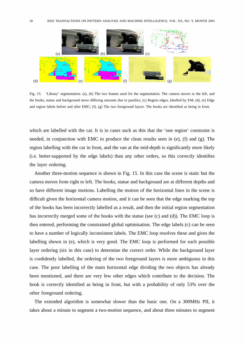


![[Carlo M. Cipolla] Les Lois Fondamentales de La Stupidite](https://static.documents.pub/doc/80x56/55cf94a3550346f57ba35fdd/carlo-m-cipolla-les-lois-fondamentales-de-la-stupidite.jpg)


![arXiv:1505.07293v1 [cs.CV] 27 May 2015 · Vijay Badrinarayanan, Ankur Handa, Roberto Cipolla Machine Intelligence Lab, Department of Engineering, University of Cambridge, UK vb292,ah781,cipolla@eng.cam.ac.uk](https://static.documents.pub/doc/80x56/5ec794057ac28100f6679570/arxiv150507293v1-cscv-27-may-2015-vijay-badrinarayanan-ankur-handa-roberto.jpg)