IEEE TRANSACTIONS ON ULTRASONICS, …jilu/papers_pdf/jilu/lu25_ieee_uffc95jul.pdfApplication of...

IEEE TRANSACTIONS ON ULTRASONICS, FERROELECTRICS, AND FREQUENCY CONTROL, VOL. 42, NO. 4, JULY 1995 649

Application of Bessel Beam forDoppler Velocity Estimation

Jian-Yu Lu, Member, IEEE, Xiao-Liang Xu, Member, IEEE, Hehong Zou, and James F. Greenleaf, Fellow, IEEE

Abstract— Limited-diffraction beams have a large depth offield and could be applied to medical imaging, tissue character-ization, and nondestructive evaluation of materials. This paperreports the application of limited-diffraction beams, specifically,the Bessel beam, to Doppler velocity estimation. The Besselbeam has the advantage that velocity estimation is less subjectto the depth of moving objects and the Doppler spectrum hasdistinct shoulders that increase the accuracy of velocity (bothmagnitude and Doppler angle) estimation in noisy environments.The shoulders of the Doppler spectrum might also help in solvingthe inverse problem, e.g., estimation of the velocity distributionin vessels.

I. INTRODUCTION

THE Doppler effect was discovered by the Austrian physi-cist, Christian Doppler in 1843 [1]. It has been applied to

electromagnetic waves [2] and medical ultrasound such as theestimation of blood flow with backscattered continuous wave(CW) [3], pulsed wave (PW) [4], imaging of blood vessels[5], and color flow mapping [6]. Recently, Doppler spectralbroadening due to the beam geometry has been analyzed [7]and applied to the estimation of the flow velocity componentthat is perpendicular to the beam axis [8]–[13].

In previous studies, beams designed to use the Dopplereffect or spectrum broadening were either plane waves orconventional focused beams. The plane wave can not definea lateral position and thus has low resolution in imaging.Conventional focused beams can produce high resolution attheir focuses but have a short depth of field and thus the shapeof their Doppler spectra may change with depth.

The first beam that can focus over a large depth wasfound in electromagnetics by Brittingham [14] and was calledfocus wave mode (FWM). The FWM was further studiedby Ziolkowski et al. [15], [16]. Limited-diffraction beams,which were originally called nondiffracting beams, were firstdiscovered by Durnin in 1987 [17]. These beams have a largedepth of field [18]–[23] and might have applications in medicalultrasonic imaging [24]–[26], tissue characterization [27], [28],and nondestructive evaluation of materials [29], and otherphysics related areas such as electromagnetics [30], [31] andoptics [32]–[40]. Because of the large depth of field of thelimited diffraction beams, theoretically, flow estimation withthese beams should be depth-independent.

Manuscript received June 27, 1994; revised November 15, 1994. This workwas supported in part by grants CA 43920 and CA 54212 from the NationalInstitutes of Health.

The authors are with the Biodynamics Research Unit, Department ofPhysiology and Biophysics, Mayo Clinic and Foundation, Rochester, MN55905 USA.

IEEE Log Number 9410105.

With the Doppler effect, one can only estimate the velocitycomponent that is parallel to the beam axis. Doppler spectrumbroadening which is caused by amplitude modulation of thereceived signal, is related to the velocity component that is per-pendicular to the beam axis. From these two components, themagnitude of velocity and its angle with the beam axis can becalculated. It has been shown that the maximum and minimumfrequency points of the Doppler spectrum of a conventionalfocused piston beam are independent of the axial distance ofa moving object [11]. However, the shape of the Dopplerspectrum may change with distance. For example, the shape ofthe Doppler spectrum of a focused piston beam is triangularonly near the focus [9]. Therefore, in a noisy environmentwhere the maximum and the minimum frequency points ofthe spectrum are difficult to measure directly, it is difficult toobtain a consistent estimation of the bandwidth of the spectrumand thus the velocity component that is perpendicular to thebeam axis over distance. Furthermore, for a focused Gaussianbeam, theoretically, there are no finite maximum and minimumfrequency points in the Doppler spectrum at the focal plane(the Fourier transform of a Gaussian function is Gaussian). Inthis case, the estimation of bandwidth and thus the transversevelocity component of a moving object depends entirely onthe shape of the spectrum.

In this paper, we apply limited-diffraction beams, specifi-cally, the Bessel beam [17], to velocity estimation using theDoppler effect. Because the Bessel beam has a large depthof field, both the shape and the maximum and minimumfrequency points of its Doppler spectrum are less dependenton the distance of moving objects. In addition, the Dopplerspectrum of the Bessel beam for an object moving at a constantvelocity has distinct shoulders representing the lower andupper boundaries of the spectrum that are related to both theangle and the magnitude of the velocity of the object. Becauseof the shoulders, the velocity vector estimation may be moreaccurate and less subject to noise. These features of the Besselbeam are derived theoretically, demonstrated with computersimulation, and verified with experiment.

In the following, we first derive the Doppler spectra of aBessel beam for various moving objects. Then we demonstratethe theoretical results with computer simulation. Experimentalresults are then reported. Finally, we give a brief discussionand conclusion.

II. THEORY

We first give the formula of a limited-diffraction beam,specifically the Bessel beam, and then derive the Dopplerspectra for various moving objects.

0885–3010/95$04.00 1995 IEEE

650 IEEE TRANSACTIONS ON ULTRASONICS, FERROELECTRICS, AND FREQUENCY CONTROL, VOL. 42, NO. 4, JULY 1995

(a)

(b)

(c)

Fig. 1. Velocity estimation with a Bessel beam. The axis of the Bessel beamis at x = 0 and y = 0. zA is the distance between the intersection of theprojection of the velocity, ~v, on the plane y = 0 and the surface of theBessel transducer. Because the Bessel beam is axially symmetric, we canalways assume that the velocity, ~v, is in parallel with the plane, y = 0. P0represents a point receiver or a point scatterer located at (x0; y0; z0) (Panel(a)). L = 50mm is either the length of a smooth line segment (Panel (b)) orthat of a line of random scatterers (Panel (c)) moving at the velocity, ~v. L iscentered at (0; 0; zA) when time t = 0. � and �1 are complementary about�. �1 is used to indicate the Doppler angle for all other figures that show apositive frequency shift when �1 < �=2.

A. Bessel Beam

One of the limited-diffraction beams, called the Besselbeam, is given by [17]

(1)

where is a complex constant that relates to the gain andinitial phase of a system (without losing generality, we assume

), represents the pressure or velocity potential ofan acoustic wave (or scalar components of an electromagneticwave), is the zeroth-order Bessel function of the firstkind, represents a point in space, ,

is the azimuthal angle in a transverseplane of the beam, is the axial distance, is time,denotes a scaling factor that determines the beam width,

, in which is the wave number,is the angular frequency and is the frequency, and

is the speed of sound in the medium.If the Bessel beam is approximately produced with a finite

aperture, it has a finite depth of field

(2)

which is much larger than that of a conventional beam (whereis the radius of a circular aperture).

B. Doppler Spectrum of Signal Measured by a Moving Receiver

We first describe the one-way Doppler spectrum in whicha point receiver moves in a Bessel beam. This simple casewill demonstrate the fundamentals to be used in the theoreticalanalysis of the two-way (pulse-echo or backscattered) Dopplerspectrum. Assume that a point receiver is located in the plane,

, moving at a velocity, , across the axis of a Besselbeam at an angle, (Fig. 1(a)). The motion of the receivercan be described with

(3)

where the coordinates, , represent the original po-sition of the receiver (at ). If we ignore the secondaryDoppler effect (the Doppler effect caused by the change ofor ) in (1), the signal received is given by

(4)

where , is the transmitted frequency,, and .

Eq. (4) can be rewritten as

(5)

From the definition of the Fourier transform [41]

(6)

and the shift and modulation theorems [42], the spectrum of(4) is given by [43]

(7)

where

(8)

For other that do not satisfy (8), . This meansthat the spectrum of the received signal (see (4)) has a finitebandwidth where the boundaries and the central frequency ofthe spectrum are related to the velocity, . In either (5) or (7),it is seen that the axial distance, , appears only in the constantphase term, , and does not affect the magnitude or the

LU et al.: APPLICATION OF BESSEL BEAM FOR DOPPLER VELOCITY ESTIMATION 651

Fig. 2. Simulated Doppler spectra of a moving point receiver (one-way) (Panels (1) to (4)) and a point scatterer (backscattered) (Panels (5) to (8)) at theplane, y = 0, in the Bessel beam with the scaling factor, � = 1202:45 m

�1, and frequency of 2.5 MHz. The point was located at x0 = 0 when t = 0.The upper and lower 4 panels are the spectra obtained with the time window, t1 = 1s and 66:7 ms, respectively. The time interval was [�t1=2; t1=2]

and was weighted with a Blackman window. The panels in the first and the third rows were obtained with the Doppler angle of 45 degrees, while thepanels in the second and the fourth rows were obtained at 60 degrees. The velocity and the axial distance, zA (see Fig. 1), of the point, P0, were 0.3m/s and 120 mm, respectively. At this velocity, the moving distance of the point was 300 mm and 20 mm for t1 = 1s and 66:7 ms, respectively. Thevertical bars show the theoretical predication of the lower and upper boundaries (dotted lines) and the frequency shift (full line) of the spectra (see (9)to (11) for a moving point receiver, and (24) and (25) for a point scatterer).

shape of the Doppler spectrum. This means that the estimationof the velocity will not be influenced by the distance of thepoint receiver if a perfect Bessel beam is used.

From (8) one obtains the lower and upper boundaries of thespectrum (abrupt cut-offs in the spectrum (Figs. 2(1) and (2))),

(9)

and

(10)

respectively, where

(11)


is the shifted central frequency,

(12)

is the frequency shift (see (8)), and

(13)

is the bandwidth of the spectrum (Figs. 2(1) and (2)), where(Fig. 1(a)) (for , the velocity has a

component that is toward the transducer and thus the frequencyshift, , is positive). Note that the bandwidth, , is nota function of the frequency of the beam, and the Dopplerspectrum has the same shape ((8) and (12)) at any centralfrequency, . This is different from that of a conventionalfocused beam where the bandwidth of the Doppler spectrumis a linear function of the central frequency [9].

Once we measure the frequency shift, , and the band-width, , the velocity of the point receiver and the anglebetween the velocity and the beam axis can be calculated

(14)

and

when (15)

or

when (16)

At , the Doppler spectrum (see (7)) is not varied.The Doppler spectrum in this case must be obtained from theFourier transform of (4) with directly,

(17)Since , the point receiver is moving directly away fromthe source (Fig. 1(a)) resulting a negative frequency shift,

, from . The magnitude of the spectrum is a function of

the position of the point receiver and theDoppler spectrum has a zero bandwidth (see the functionin (17)).

If , the Doppler spectrum can be obtained directlyfrom (7)

(18)

and one sees no shift in the central frequency but a maximumbandwidth of the Doppler spectrum, .

Equation (7) has the following property

(19)

where

otherwise(20)

is obtained from (7) with . This implies that theDoppler spectrum for a moving point receiver is under thecurve defined by (20) which is peaked at the spectrumboundaries and has a minimum at the central frequency,

(Figs. 2(1) and (2)). The peaks at the boundariesmakes it easy to determine the bandwidth of the spectrum andthus the Doppler angle (see (15)).

It is noted from (4) that if , the maximum amplitudeof the received signal will decrease rapidly and monotonicallywith . This means that the signals received off the plane,

, may be negligible.

C. Doppler Spectrum from a Moving Point Scatterer

If the Bessel transducer in Fig. 1 is used as both a transmitterand a receiver [25], the received signal that is backscatteredfrom a point scatterer is given by [44]

(21)

where the subscript “b” represents “backscattered”. TheDoppler spectrum (Figs. 2(5) and (6)) of the received signalis the Fourier transform of (21)

(22)where “*” represents the convolution with respect to , and

(23)

which is the Fourier transform of the term inside the squarebracket in (21) and is similar to (7).

Because is convolved with itself in (22), thebandwidth of the backscattered Doppler signal is doubled fromthat of the signal of a moving point receiver (see (13)), i.e.,

(24)

The central frequency of the backscattered Doppler signal canbe obtained from the expression of in (22), i.e.,

(25)

The equations for calculating the lower and upper boundariesof the backscattered Doppler spectrum are the same as (9)


Fig. 3. Simulated Doppler spectra of the backscattered signals from a moving smooth line segment of length of 50 mm (see Fig. 1) in the Bessel beamdescribed in Fig. 2. The line segment was in the plane, y = 0. Its velocity was 0.3 m/s and the axial distance, zA, was 120 mm. A larger Blackman-weightedtime window, t1 = 1s, as in Fig. 2 was applied to the backscattered signals. Panels (1) to (10) correspond to the Doppler angle of 45 to 90 degreeswith an increment of 5 degrees. The spectra at 85 and 90 degrees were distorted because a 75 Hz wall filter (high-pass filter) was added. The verticalbars show the theoretical predication of the lower and upper boundaries (dotted lines) and the frequency shift (full line) of the spectra (they are the sameas those of a point scatterer in Fig. 2 and are obtained from (24) and (25)).

and (10). However, and in those equations need to bereplaced with and in (24) and (25).

D. Doppler Spectrum from a Moving Line Segment

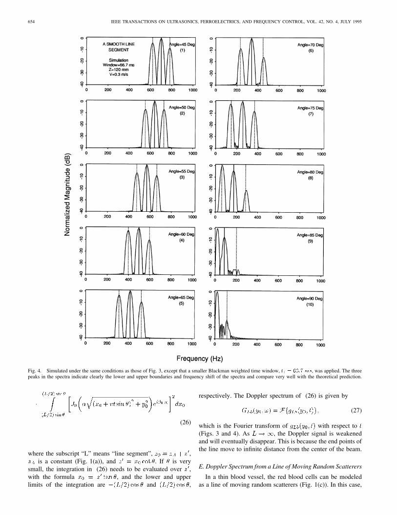
For a smooth line that is infinitely long and moves in thedirection of the line, there will be no Doppler shift. However,if the line has a finite length, one will see the motion of the endpoints of the line and thus may obtain Doppler spectrum. Inthis case, we found an interesting spectrum that is composed

of three peaks corresponding almost exactly to the centralfrequency, and the lower and upper boundaries of the spectrum(Fig. 4). This might be used to detect the velocity of a smoothjavelin in sports or a missile.

If point scatterers are uniformly distributed in a line seg-ment (Fig. 1(b)) of length , the backscattered signal is anintegration of (21)


Fig. 4. Simulated under the same conditions as those of Fig. 3, except that a smaller Blackman weighted time window, t1 = 66:7ms, was applied. The threepeaks in the spectra indicate clearly the lower and upper boundaries and frequency shift of the spectra and compare very well with the theoretical prediction.

(26)

where the subscript “L” means “line segment”, ,is a constant (Fig. 1(a)), and . If is very

small, the integration in (26) needs to be evaluated over ,with the formula , and the lower and upperlimits of the integration are and ,

respectively. The Doppler spectrum of (26) is given by

(27)

which is the Fourier transform of with respect to(Figs. 3 and 4). As , the Doppler signal is weakenedand will eventually disappear. This is because the end points ofthe line move to infinite distance from the center of the beam.

E. Doppler Spectrum from a Line of Moving Random Scatterers

In a thin blood vessel, the red blood cells can be modeledas a line of moving random scatterers (Fig. 1(c)). In this case,


Fig. 5. Simulated under the same conditions as those of Fig. 4, except that the moving smooth line segment was replaced with a line of moving randomscatterers. 2048 scatterers were positioned randomly along the 50 mm line (Fig. 1(c)) with a uniform distribution. The spectra were obtained by averagingthe magnitudes of 40 independent Doppler spectra from lines of moving random scatterers.

(26) must be evaluated with a summation

(28)

where the subscript “R” means “random,” is an index of therandom scatterers, , and . TheDoppler spectrum of the signal from a line of moving random

scatterers is the Fourier transform of (28) with respect to time, i.e., .

III. SIMULATION

In the following simulation, we assume that a perfect Besselbeam ((1)) is used, where the scaling factor, , speed of sound,, and frequency, , are 1202 m 1, 1500 m/s, and 2.5 MHz,

respectively. We also assume that the objects are movingin the plane . In addition, we ignore the modulationterm, , that shifts the Doppler spectrum by the carrierfrequency, (consider only the frequency components caused


by motion). To avoid abrupt truncation in time, a Blackmanwindow [42] of duration, , and peaked atis multiplied with the received signal before taking the Fouriertransform. The sampling frequency is 2048 Hz and the totalsamples for the digital Fourier transform (DFT) [42] is 2048.This means that the frequency resolution of the spectrum is1 Hz. The low frequency components of the spectrum thatcorrespond to the slow motion of objects are suppressed by a75 Hz wall filter (a half-width Blackman window that is addedto the frequency components that are lower than 75 Hz). It isnoted that the lateral axes of the Doppler spectra in all thefigures in this paper represent the shifted frequency fromand the Doppler angles are referred to in Fig. 1, whichgives a positive frequency shift.

The magnitude of the Doppler spectra ((7) or (20)) of thesignal from a moving receiver located in the plane, ,with the sampling time, , is shown in Figs. 2(1)( ) and 2(2) ( ) (assume that at ,the receiver is at ). For a shorter sampling time,

, which corresponds to a displacement of 20mm of the receiver when moving at a velocity of 0.3 m/s,the Doppler spectra are blurred (Figs. 2(3) ( ) and2(4) ( )). The magnitude of the Doppler spectra of thesignal (see (21)) backscattered from a moving point scattereris shown in Figs. 2(5) to 2(8) that correspond to Figs. 2(1) to2(4), respectively.

The magnitude of the Doppler spectra of the signal (see(26)) backscattered from a moving smooth line segment(Fig. 1) is shown in Figs. 3 and 4, which correspond tothe time window, and , respectively. At

, the line segment is centered at (Fig. 1(b)). It isinteresting to note that with the smaller time window (Fig. 4),the three peaks in the spectra coincide almost exactly with thetheoretical prediction of the frequency shift, lower and upperboundaries (calculated from (24) and (25)), respectively.Even with a larger window (Fig. 3), the central peak and theshoulders of the spectra are predicted very well by the theory.For the signal backscattered from a line of moving randomlydistributed scatterers (see (28)), the shape of the spectrum mayalso be random. Therefore, to obtain a meaningful spectrum,the magnitude of a number of independent Doppler spectramust be averaged. Magnitudes of 40 Doppler spectra wereaveraged from moving random scatterers and are shown inFig. 5, where a smaller time window, , is used.

IV. EXPERIMENT

To verify the theoretical analysis, we designed a Dopplerflow phantom (Fig. 6) [45]. A thin sewing thread [7] (about 0.1mm in diameter) was mounted on the phantom and was usedas a line of moving random scatterers. A 10–element, 50 mmdiameter, 2.5 MHz central frequency annular array transducer[24] was used to produce either a Bessel beam (with the scalingfactor of ) or a focused Gaussian beam (thefull width at half maximum (FWHM) of the aperture weightingis 25 mm and the focal length is 120 mm (with a plexiglasslens)) [25]. The backscattered signals from the sewing threadwere received with the same transducer, weighted the same

Fig. 6. A Doppler phantom made in our laboratory. A sewing thread ofabout 70.5 cm long and 0.1 mm in diameter was moved by a DC motor.The speed of the motor was controlled by the DC voltage. The position ofthe phantom was adjusted so that the part of the thread on the bottom of thephantom passes through the axis (in the plane y = 0) of the Bessel beam(� = 1202:45 m

�1) or the focused Gaussian beam (FWHM = 25 mm atthe transducer surface and the focal length F = 120 mm (with a plexiglasslens)) that was produced by a 10–element, 50 mm diameter, and 2.5 MHzannular array. The phantom can be rotated around the holding rod to adjustthe Doppler angle. The beams were perpendicular to the figure.

way as it was in transmit. The position of the phantom wasadjusted so that the sewing thread passed through the centerof the beams (the sewing thread was in the plane ).The sewing thread was driven by a DC motor and its velocitywas controlled by adjusting the DC voltage applied to themotor. The phantom can be rotated around its axis to adjustthe Doppler angle, (Fig. 1).

A block diagram of the experiment system is shown in Fig.7. In the experiment, a 2.5 MHz, 20 s tone-burst producedby a polynomial waveform synthesizer (ANALOGIC DATA2045) was amplified to drive the transducer. The first and thelast 5 s of the tone-burst were weighted by a rising and fallingBlackman window. The weighting reduces the sidelobes ofthe spectrum dramatically while maintaining the narrow bandcharacteristics of the tone-burst.

To obtain a demodulated backscattered signal, only one da-tum was acquired by the A/D converter for each transmissionof the tone-burst. The delay time between the transmission andthe datum acquisition was fixed. If the object that backscattersthe incident wave does not move, the acquired datum fromeach transmission will be the same (no frequency shift).However, if the object moves at a constant speed towardsthe transducer, the received tone-burst will progressively shiftforward in time for each transmission. This change of receiveddata contains the information of the motion. As long as thetransmission triggering frequency (pulse repetition frequencyor PRF) is high enough so that no aliasing occurs (PRF =2048 Hz in the experiment), the velocity and the Dopplerangle can be estimated from the Doppler spectrum ((14)and (16)).


Fig. 7. A block diagram of the Doppler experiment. A polynomial waveformsynthesizer (DATA 2045) produced a 2.5 MHz, 20 �s, and Blackman-windowweighted tone-burst that was amplified to drive the annular array transducerto produce either a Bessel or focused Gaussian beam. Echoes received wereamplified, aperture weighted in the same way as in the transmit, and digitizedby an A/D converter at a fixed delay time that was chosen to sample apoint at the middle of the tone-burst. Only one sample was acquired foreach transmission of the tone-burst. Trigger pulses for beam transmissionswere produced by a function generator (EXACT 7260) at 2048 Hz (the pulserepetition frequency) that was monitored by the Timer/Counter (HP 5327A).

To match the simulation (Fig. 5), magnitudes of about 40independent Doppler spectra from the sewing thread wereaveraged and the Blackman time window of the duration,

, where , was applied to the signalsbefore the Fourier transform.

V. RESULTS

The magnitude of the Doppler spectra of the backscatteredsignals from a line of moving random scatterers (sewingthread) is shown in Figs. 8 and 9, for the Bessel and focusedGaussian beams (see last section), respectively. The spectraare obtained at two depths (120 mm and 150 mm). Thespectrum obtained with the focused Gaussian beam showsmore variation with depth. The signals were processed in thesame manner described in the last section.

To demonstrate the Doppler spectra of the backscatteredsignal from a blood vessel that has a parabolic velocitydistribution, we placed the sewing thread at an axial distanceof , and obtained the backscattered signalfrom 11 positions from 5 mm to 5 mm in 1 mm steps.Here we assume that the blood vessel is very thin in thedirection and is located in the plane, . This assumptionis reasonable because the amplitude of the Bessel function in(4) or (21) drops quickly as increases. The velocity of

the sewing thread was varied using the following parabolicformula

(29)

where is the maximum velocity of the red blood cells(0.3 m/s) and is the radius of the blood vessel (6 mm). Fromthis equation, it is seen that each velocity corresponds to two

depths (except at ). Therefore, the backscattered sig-nals from two depths are superposed coherently (rf summation)to represent the signal at one velocity. The Doppler spectra ofthe signals from the above 6 different velocities are shown inPanels (1) to (6) of Fig. 10. To obtain the spectrum of signalsfrom the entire vessel, the rf signals for the 6 velocities aresummed (see Panel (7) of Fig. 10).

VI. DISCUSSION

From the simulations and the experiments, we have shownthat the Doppler spectra obtained with Bessel beams haveshoulders that are different from those obtained with con-ventional focused beams [9]. These shoulders indicate clearlythe bandwidth of the Doppler spectrum and correspond tothe theoretical prediction very well. The central frequencycan be either determined from the peak of the spectrum(for backscattered signals) or calculated from the shoulders.Therefore, from the shoulders, the velocity of object and theDoppler angle can be estimated if the object is moving in aconstant speed during the data acquisition time, . Because theshoulders are relatively high in amplitude (around 10-dB ofthe peak of the Doppler spectrum (for backscattered signals)),their identification is less sensitive to noise than when using aconventional focused beam where there is no shoulder at all.This may increase the accuracy of the estimation of magnitudeand angle of velocity. In addition, because the Bessel beamhas a large depth of field even if it is produced with a finiteaperture (see (2)) [17], [24], [25], its Doppler spectra have lessvariation with depth as compared to a focused Gaussian beam(Figs. 8 and 9).

Although the experimental study on the moving sewingthread has shown the major features of the Doppler spectrumpredicted by the theory and simulation, it is preliminary. TheDoppler spectrum obtained from the experiment contains abroadband noise (Figs. 8 to 10) produced from our multi-channel receiver. The differences between the results of amoving thread experiment with the Bessel beam (Fig. 8) andthe simulation of a line of moving random scatterers (Fig.5) are caused by the aperture weighting errors due to highcross talk among our transmit amplifiers, the truncation of theBessel beam to a finite diameter, say, 50 mm, the specularreflections from trapped air bubbles and regular patterns inthe thread, and the nonuniform thickness of the thread. Thedeviation of the shape of the Doppler spectrum (Fig. 9) fromthat of Gaussian is also caused by the nonideal Gaussian beamdue to the aperture weighting errors.

The simulation demonstrated that the Doppler spectrumof signal from a moving receiver has only shoulders andno central peak (Figs. 2(1) to 2(4)) producing more distinctshoulders. In a pulse-echo system, such Doppler spectra can beproduced by using a Bessel beam in transmit and an unfocusedplanar aperture in receive or vice versa (the role of theunfocused planar receiver or transmitter is to shift the Dopplerspectrum obtained with the Bessel beam by about ,where is the central frequency of the transmitting beam).However, the broad spatial response of the unweighted planar


Fig. 8. Measured Doppler spectra of the backscattered signals for a moving sewing thread (Fig. 6) that represents a line of moving random scatterers. Thethread passed through the axis (in the plane y = 0) of the Bessel beam that was produced by the transducer described in Fig. 6, and was at two axial distances,zA = 120 mm (full line) and 150 mm (dotted line), respectively. A 2.5 MHz, 20 �s, and Blackman-weighted tone-burst was used to excite the transducerand the received signals were also weighted with the Blackman window with the time duration, t1 = 66:7 ms. The velocity of the thread was obtained bymeasuring the time of the node of the thread passing through a reference point in space and dividing the length of the thread with the time (10 revolutions wereused to reduce the error). The Doppler angle in each panel was calculated from the spectrum and was roughly from 45 (Panel (1)) to 90 (Panel (10)) degrees atan increment of 5 degrees. A 75 Hz wall filter was added to the spectra to reduce the large signals from the slow motion of the thread. The vertical bars showthe theoretical predication of the lower and upper boundaries (dotted lines) and the frequency shift (full line) of the spectra (calculated from (24) and (25)).

aperture may reduce the spatial resolution and increase thesidelobes.

Estimation of the velocity distribution in a blood vessel isimportant for flow estimation. The current method is to choosea very small range cell (short pulse duration) and place therange cell within different positions of a blood vessel to obtaina rough estimation of the velocity distribution. It is apparent

that the smaller the range cell is, the broader the bandwidthof the impinging beams will be and thus the less accurate thevelocity estimation. Therefore, it is desirable that one couldestimate the velocity distribution from the Doppler spectrumwith a larger range cell. The Doppler spectrum obtained withthe Bessel beam has the feature that the spectrum of eachvelocity component has shoulders and the bandwidth of the


Fig. 9. Doppler spectra obtained with the same procedures as those in Fig. 8, except that a focused Gaussian beam (FWHM = 25 mm at the transducersurface and the focal length F = 120 mm (with a plexiglass lens)) was used. The vertical bars represent the shift of the central frequency.

spectrum depends only on the velocity (Fig. 10). Thus thespectrum from a group of scatterers traveling at differentspeeds will be a summation of nonorthogonal basis functions.This might be of help in the estimation of velocity distributions(an inverse problem) and could be studied in the future.

For medical applications, more complicated situations suchas the use of short pulses (broadband probing signals), shortersampling time (smaller number of samples in color flowmapping [6]), and existence of pulsatile flow will have to beconsidered. The solution to these problems might be a trade-off between the accuracy of the velocity estimation and theabove parameters. Time domain velocity estimation might bea better approach to some of these problems [46].

VII. CONCLUSION

Limited-diffraction beams have a large depth of field. Theycould be applied to medical imaging [24]–[26], tissue charac-terization [27], [28], and nondestructive evaluation (NDE) ofmaterials [29]. This paper has shown that limited-diffractionbeams, especially, the Bessel beam, can also be applied tovelocity estimation using the Doppler effect. Application ofthe Bessel beam to velocity estimation has the advantagethat its Doppler spectrum has little depth dependence andhas distinct shoulders that may increase the accuracy of thevelocity magnitude and angle estimates in noisy environments,as compared to conventional focused beams. The distinct


Fig. 10. Measured Doppler spectra of the backscattered signals for a vessel of parabolic flow (the velocity distribution on a cross section of the vessel is aparabolic function) in the Bessel beam produced by the transducer described in Fig. 6. The vessel was assumed to be very thin and located in the plane, y = 0,with its center located at the axial distance, zA = 120 mm. The diameter of the vessel was 12 mm, and there were only 6 different velocities that span adistance of 10 mm with an increment of 1 mm (except at the center of the vessel, each velocity corresponds to two spatial positions in the parabolic flow).The Doppler angle was 70 degrees. Panels (1) to (6) correspond to 6 velocities in a parabolic velocity distribution, i.e., v = 0.3, 0.291, 0.266, 0.225, 0.173,and 0.0915 m/s, respectively. For Panels (2) to (6), the backscattered signals from two positions were summed coherently to obtain the Doppler spectra. TheDoppler spectrum of the backscattered signals from the entire vessel is shown in Panel (7) and was obtained by coherently summing the signals of the above6 panels. The vertical bars show the theoretical prediction of the lower and upper boundaries (dotted lines) of the spectra and the frequency shift (solid lines).

shoulders of the Doppler spectrum produced by the Besselbeam might help in estimating distributions of velocities inblood vessels.

ACKNOWLEDGMENT

The authors thank Mr. Randall R. Kinnick for making theDoppler phantom. The secretarial assistance of Elaine C.Quarve is appreciated.

REFERENCES

[1] C. Doppler, “Ueber das farbige Licht der Doppelsterne und einiger an-derer Gestirne des Himmels,” Abhandlungen der Koniglich BohmischenGesellschaft der Wissenschaften, vol. 2, no. 5, pp. 465–482, 1843.

[2] E. J. Jonkman, “Doppler research in the nineteenth century,” UltrasoundMed. Biol., vol. 6, no. 1, pp. 1–5, Jan. 1980.

[3] D. L. Franklin, W. Schlegel, R. F. Rushmer, “Blood flow measured byDoppler frequency shift of back-scattered ultrasound,” Sci., vol. 134,pp. 564–565, 1961.


[4] P. N. T. Wells, “A range-gated ultrasonic Doppler system," Med. Biol.Eng., vol. 7, pp. 641–652, 1969.

[5] J. M. Reid and M. P. Spencer, “Ultrasonic Doppler technique forimaging blood vessels,” Sci., vol. 176, pp. 1235–1236, 1972.

[6] P. A. Magnin, “A review of Doppler flow mapping techniques,” in IEEE1987 Ultrason. Symp. Proc., 87CH2492–7, vol. 2, pp. 969–977, 1987.

[7] V. L. Newhouse, E. S. Furgason, G. F. Johnson, and D. A. Wolf, “Thedependence of ultrasound Doppler bandwidth on beam geometry,” IEEETrans. Sonic. Ultrason., vol. SU-27, pp. 50–59, 1980.

[8] P. A. J. Bascom, R. S. C. Cobbold, and B. H. M. Roelofs, “Influenceof spectral broadening on continuous wave Doppler ultrasound spectra:a geometric approach,” Ultrasound Med. Biol., vol. 12, pp. 387–395,1986.

[9] V. L. Newhouse, D. Censor, T. Vontz, J. A. Cisneros, and B. B.Goldberg, “Ultrasound Doppler probing of flows transverse with respectto beam axis,” IEEE Trans. Biomed. Eng., vol. BME-34, no. 10, pp.779–789, Oct. 1987.

[10] D. Censor, V. L. Newhouse, T. Vontz, and H. V. Ortega, “Theoryof ultrasound Doppler-spectra velocimetry for arbitrary beam and flowconfigurations,” IEEE Trans. Biomed. Eng., vol. 35, no. 9, pp. 740–751,Oct. 1988.

[11] V. L. Newhouse and J. M. Reid, “Invariance of Doppler bandwidth withflow axis displacement,” in IEEE 1990 Ultrason. Symp. Proc., 1990, vol.2, pp. 1533–1536.

[12] P. Tortoli, G. Guidi, V. Mariotti, and V. L. Newhouse, “Experimen-tal proof of Doppler bandwidth invariance,” IEEE Trans. Ultrason.,Ferroelec., Freq. Contr., vol. 39, no. 2, pp. 196–203, Mar. 1992.

[13] P. Tortoli, G. Guidi, V. Mariotti, and V. L. Newhouse, “Invariance ofthe Doppler bandwidth with range cell size above a critical beam-to-flow angle,” IEEE Trans. Ultrason., Ferroelec., Freq. Cont., vol. 40, no.4, pp. 381–386, Jul. 1993.

[14] J. N. Brittingham, “Focus wave modes in homogeneous Maxwell’sequations: transverse electric mode,” J. Appl. Phys., vol. 54, no. 3, pp.1179–1189, 1983.

[15] R. W. Ziolkowski, “Exact solutions of the wave equation with complexsource locations,” J. Math. Phys., vol. 26, no. 4, pp. 861–863, Apr. 1985.

[16] R. W. Ziolkowski, D. K. Lewis, and B. D. Cook, “Evidence of localizedwave transmission,” Phys. Rev. Lett., vol. 62, no. 2, pp. 147–150, Jan.1989.

[17] J. Durnin, “Exact solutions for nondiffracting beams. I. The scalartheory,” J. Opt. Soc. Am., vol. 4, no. 4, pp. 651–654, 1987.

[18] Jian-yu Lu, Hehong Zou, and J. F. Greenleaf, “Biomedical ultrasoundbeam forming,” Ultrasound Med. Biol. vol. 20, no. 5, pp. 403–428,July, 1994.

[19] Jian-yu Lu and J. F. Greenleaf, “Nondiffracting X waves — exactsolutions to free-space scalar wave equation and their finite aperturerealizations,” IEEE Trans. Ultrason., Ferroelec., Freq. Cont., vol. 39,no. 1, pp. 19–31, Jan. 1992.

[20] , “Experimental verification of nondiffracting X waves,” IEEETrans. Ultrason., Ferroelec., Freq. Cont., vol. 39, no. 3, pp. 441–446,May 1992.

[21] D. K. Hsu, F. J. Margetan, and D. O. Thompson, “Bessel beam ultrasonictransducer: fabrication method and experimental results,” Appl. Phys.Lett., vol. 55, no. 20, pp. 2066–2068, Nov. 1989.

[22] J. A. Campbell and S. Soloway, “Generation of a nondiffracting beamwith frequency independent beam width,” J. Acoust. Soc. Am., vol. 88,no. 5, pp. 2467–2477, Nov. 1990.

[23] R. Donnelly, D. Power, G. Templeman, and A. Whalen, “Graphicsimulation of superluminal acoustic localized wave pulses” IEEE Trans.Ultrason., Ferroelec., Freq. Cont., vol. 41, no. 1, pp. 7–12, 1994.

[24] Jian-yu Lu and J. F. Greenleaf, “Ultrasonic nondiffracting transducerfor medical imaging,” IEEE Trans. Ultrason., Ferroelec., Freq. Cont.,vol. 37, no. 5, pp. 438–447, Sept. 1990.

[25] , “Pulse-echo imaging using a nondiffracting beam transducer,”Ultrasound Med. Biol., vol. 17, no. 3, pp. 265–281, May 1991.

[26] Jian-yu Lu, Tai K. Song, Randall R. Kinnick, and J. F. Greenleaf, “Invitro and in vivo real-time imaging with ultrasonic limited diffractionbeams,” IEEE Trans. Med. Imag., vol. 12, no. 4, pp. 819–829, Dec.1993.

[27] Jian-yu Lu and J. F. Greenleaf, “Evaluation of a nondiffracting trans-ducer for tissue characterization,” in IEEE 1990 Ultrason. Symp. Proc.,1990, vol. 2, pp. 795–798.

[28] , “Diffraction-limited beams and their applications for ultrasonicimaging and tissue characterization,” in Proc. SPIE, 1992, vol. 1733,pp. 92–119.

[29] , “Producing deep depth of field and depth-independent resolutionin NDE with limited diffraction beams,” Ultrason. Imag., vol. 15, no.

2, pp. 134–149, Apr. 1993.[30] R. W. Ziolkowski, “Localized transmission of electromagnetic energy,”

Phys. Rev. A., vol. 39, no. 4, pp. 2005–2033, Feb. 15, 1989.[31] R. Donnelly and R. W. Ziolkowski, “Designing localized waves,” Proc.

Royal Soc. Lond., A, vol. 440, pp. 541–565, 1993.[32] J. Durnin, J. J. Miceli, Jr., and J. H. Eberly, “Diffraction-free beams,”

Phys. Rev. Lett., vol. 58, no. 15, pp. 1499–1501, Apr. 1987.[33] A. Vasara, J. Turunen, and A. T. Friberg, “Realization of general

nondiffracting beams with computer-generated holograms,” J. Opt. Soc.Am. A, vol. 6, no. 11, pp. 1748–1754, 1989.

[34] G. Indebetow, “Nondiffracting optical fields: some remarks on theiranalysis and synthesis,” J. Opt. Soc. Am. A, vol. 6, no. 1, pp. 150–152,Jan. 1989.

[35] F. Gori, G. Guattari, and C. Padovani, “Model expansion for J0-correlated Schell-model sources,” Optics Commun., vol. 64, no. 4, pp.311–316, Nov. 1987.

[36] , “Bessel-Gaussian beams,” Optics Commun., vol. 64, no. 6, pp.491–495, Dec. 1987.

[37] K. Uehara and H. Kikuchi, “Generation of near diffraction-free laserbeams,” Appl. Physics B, vol. 48, pp. 125–129, 1989.

[38] L. Vicari, “Truncation of nondiffracting beams,” Optics Commun., vol.70, no. 4, pp. 263–266, Mar. 1989.

[39] M. Zahid and M. S. Zubairy, “Directionally of partially coherent Bessel-Gauss beams,” Optics Commun., vol. 70, no. 5, pp. 361–364, Apr.1989.

[40] S. Y. Cai, A. Bhattacharjee, and T. C. Marshall, “’Diffraction-free’optical beams in inverse free electron laser acceleration,” NuclearInstruments and Methods in Physics Research, Section A: Accelerators,Spectrometers, Detectors, and Associated Equipment, vol. 272, no. 1–2,pp. 481–484, Oct. 1988.

[41] R. Bracewell, The Fourier Transform and Its Applications. New York:McGraw-Hill, 1965, ch. 4 and 6.

[42] A. V. Oppenheim and R. W. Schafer, Digital Signal Processing. En-glewood Cliffs, NJ: Prentice-Hall, 1975, ch. 1 and 5.

[43] I. S. Gradshteyn and I. M. Ryzhik, Table of Integrals, Series, andProducts.New York: Academic Press, 1980, ch. 6 and 17.

[44] J.-Y. Lu and J. F. Greenleaf, “A study of sidelobe reduction for limiteddiffraction beams,” in IEEE 1993 Ultrason. Symp. Proc., 1993, vol. 2,pp. 1077–1082.

[45] A. R. Walker, D. J. Phillips, and J. E. Powers, “Evaluating Dopplerdevices using a moving string test target,” J. Clin. Ultrasound, vol. 10,pp. 25–30, Jan. 1982.

[46] A. Hein and W. D. O’Brien, “Current time-domain methods for as-sessing tissue motion by analysis from reflected ultrasound echoes—areview,” IEEE Trans. Ultrason., Ferroelec., Freq. Cont., vol. 40, no. 2,pp. 84–102, Mar. 1993.

Jian-Yu Lu (M’88) received the B.S. degreein electrical engineering in 1982 from FudanUniversity, Shanghai, China, the M.S. degree in1985 from Tongji University, Shanghai, Chinaand the Ph.D. degree from Southeast University,Nanjing, Ching.

He is currently an Associate Consultnat atBiodynamics Research Unit, Department ofPhysiolofy and Biophysics, Mayo Clinic andFoundation, Rochester, MN, and he is an AssistantProfessor at the Biodynamics Research Unit at

the Mayo Medical School. Previuslu, he was a Research Assoicate atthe Biodynamic Unit, and from 1988 to 1990, he was a Post-DoctoralResearch Fellow. Prior to that, he was a faculty member of the Departmentof Biomedical Engineering, Southeast University, adn worked with ProfessorYu Wei. His research interests are in acoustical imaginag and tissuecharacterization, medical ultrasonic transducers, and nondiffracting wavetransmission.

Dr. Lu is a member of the IEEE UFFC Society, the American Institute ofUltrasound in Medicine, and Sigma Xi.


Xiao-Liang Xu (S’88–M’92) received the B.S. andM.S. degrees from Zhejiang University, Hangzhou,China, in 1982 and 1984, respectively, and the Ph.D.degree from the University of Minnesota, MN, in1991, all in electrical engineering.

From 1984 to 1986 he was with the Departmentof Electrical Engineering at Zhejiang Universityin China. From 1987 to 1991 he was a ResearchAssociate at the University at the University ofMinnesota. From 1991 to 1993 he was a Post-Doctoral Fellow at the VA Medical Center and

University of Minnesota, MN. Since 1993 he has been a Research Associateat the Mayo Clinic, Rochester, MN. His research interests include medicalimaging systems, image analysis, biomedical signal processing, statisticalsignal processing, and spectum analysis.

Hehong Zou received the B.Sc. degree from theBeijing University of Science and technology, Bei-jing, China, in 1985, the M.S. degree from theUniversity of Wisconsin, Milwaukee, WI, in 12989,and the Ph.D. degree from the University of Min-nesota, Minneapolis, MN, in 1993, all in electricalengineering.

From 1985 to 1986 he was an Engineer with theBeijing Institute of Control Engineering, Beijing,China. From 1987 to 1992 he was a Research As-sistant at the University of Minnesota, Minneapolis,

MN, and in 1992 he was a part-time software programmer at ProReHab Inc.,Roseville, MN, and in 1993 he was a Research Fellow in the Department ofPhysiology and Biophysics, Mayo Foundation, Rochester, MN. He is currentlyworking at Rosemount Inc., Chanhassen, MN.

James F. Greenleaf (M’73–SM’84–F’88) receivedthe B.S. degree in engineering science in 1968from Purdue University, West Lafayette, IN, and thePh.D. degree in engineering science in 1970 fromthe Mayo Graduate School of Medicine, Rochester,MN and Purdue University.

He is a Professor of biophysics and medicineat the Mayo Medical School and a Consultantat the Biodynamics Research Unit, Department ofPhysiology, Biophysics, and Cardiovascular Diseaseand Medicine, Mayo Foundation. His special field

of interest is in ultrasonic biomedical imaging science. he has published morethan 150 articles and edited four books.

Dr. Greenleaf has served on the IEEE Technical Committee of the Ultra-sonics Symposium since 1985. He served on the IEEE/UFFC Subcommitteefro the Ultrasonics in Medicine/IEEE Measurement Guide Editors, and on theIEEE Medical Ultrasound Committee. He is the President of the IEEE UFFCSociety. He holds five patents and is the recipient of the 1986 J. HolmesPioneer Award from the American Institute of Ultrasound in Medicine. He isa Fellow of the AUIM. He is also the Distinguished Lecturer for the IEEEUFFC Society for 1990–1991.

Date post:	20-May-2018
Category:	Documents
Upload:	ngonguyet
View:	218 times
Download:	2 times

IEEE TRANSACTIONS ON ULTRASONICS, …jilu/papers_pdf/jilu/lu25_ieee_uffc95jul.pdfApplication of...

Documents