IEEE TRANSACTIONS ON VEHICULAR TECHNOLOGY, 2019 1

Fast Solving Method Based on LinearizedEquations of Branch Power Flow for Coordinated

Charging of EVs (EVCC)Jian Zhang, Mingjian Cui, Senior Member, IEEE, Bing Li, Hualiang Fang, and Yigang He, Member, IEEE

Abstract—Reported researches on smart charging methodshave the disadvantages of low calculation efficiency or havenot simultaneously taken the three-phase imbalance, voltage andpower flow constraints into account. It is an important topicto improve the computational speed to meet the online rollingoptimization requirement for EVCC problems. In this paper,the branch power flow equations of balanced and unbalanceddistribution system are derived. The linearization methods forthe nonlinear terms of the branch power flow equations areproposed. Two stages linear programming (LP) is introduced forEVCC to minimize the total charging costs of the holders wherethree-phase imbalance, charging demand, voltage and powerflow constraints have been taken into account. Via ignoring thenonlinear terms of the branch power flow equations, the firststage LP is formulated to calculate the estimated branch powerand node voltages as the initial points for linearizing the nonlinearterms of branch power flow equations. The second stage LP isformulated to calculate the optimal charging power using thelinearized branch power flow equations. Four case studies showthat the proposed method without the compromise of precisionis significantly faster than state-of-the-art works with respect tothe computational speed.

Index Terms—Branch flow, distribution system, coordinatedcharging, electric vehicles (EVs), linear programming.

NOMENCLATURE

A. Sets:

N Buses of distribution system excluding the rootnode.

ε Line segments of distribution system.Hk Child nodes of node k.

B. Constants:

rik Resistance of line segment (i, k) for balanced dis-tribution system.

xik Reactance of line segment (i, k) for balanced distri-bution system.

zik Impedance of line segment (i, k) for balanced dis-tribution system.

rik Resistance matrix of line segment (i, k) for unbal-anced distribution system, a 3× 3 matrix.

J. Zhang, B. Li, and Y. He are with the School of Electrical Engineeringand Automation, Hefei University of Technology, Hefei, Anhui, 230009China; Y. He is also with the School of Electrical Engineering, WuhanUniversity, Wuhan, Hubei, 430072 China (e-mail: 17775357967@163.com;libinghnu@163.com; 18655136887@163.com).

M. Cui is with the Department of Electrical and Computer Engi-neering, Southern Methodist University, Dallas, TX, 75275 USA (e-mail:mingjian.cui@ieee.org).

H. Fang is with the School of Electrical Engineering, Wuhan University,Wuhan, Hubei, 430072 China (e-mail: hlfang@whu.edu.cn).

Manuscript received, 2019.

xik Reactance matrix of line segment (i, k) for unbal-anced distribution system, a 3× 3 matrix.

zik Impedance matrix of line segment (i, k) for unbal-anced distribution system, a 3× 3 matrix.

pdk0 Active power of constant power load at node k for

balanced distribution system.qdk0 Reactive power of constant power load at node k

for balanced distribution system.pdkz0 Active power of constant impedance load at node

k for balanced distribution system when voltagemagnitude is 1.0 p.u.

qdkz0 Reactive power of constant impedance load at node

k for balanced distribution system when voltagemagnitude is 1.0 p.u.

pdk0 Active power of constant power load at node k for

unbalanced distribution system, a 3× 1 vector.qdk0 Reactive power of constant power load at node k

for unbalanced distribution system, a 3× 1 vector.pdkz0 Active power of constant impedance load at node k

for unbalanced distribution system, a 3× 1 vector.qdkz0 Reactive power of constant impedance load at node

k for unbalanced distribution system, a 3×1 vector.K Total number of EVs with three-phase charging

mode.M Total number of EVs with single-phase charging

mode.t1 Optimization start time.tmax Optimization end time.β Connecting phase for EVs with single-phase charg-

ing mode.PEVk,max Charging power for the kth EV with three-phase

charging mode.PEVm,max Charging power for the mth EV with single-phase

charging mode.∆t Time interval of optimization.η Charging efficiency.Einik Initial energy of the kth EV with three-phase charg-

ing mode.Einim Initial energy of the mth EV with single-phase

charging mode.Ecapk Battery capacity of the kth EV with three-phase

charging mode.Ecapm Battery capacity of the mth EV with single-phase

charging mode.tks Charging start time for the kth EV with three-phase

charging mode.tke Charging end time for the kth EV with three-phase

charging mode.

IEEE TRANSACTIONS ON VEHICULAR TECHNOLOGY, 2019 2

tms Charging start time for the mth EV with single-phasecharging mode.

tme Charging end time for the mth EV with single-phasecharging mode.

Umin Lower limit for voltage magnitude square.Umax Upper limit for voltage magnitude square.Pmaxik,α,t Maximum active power of line segment (i, k) for

phase α in time interval t.Pmax

T,α,t Maximum active power of distribution transformerfor phase α in time interval t.

Pik0 Initial active power of line segment (i, k) for lin-earization in balanced distribution system.

Qik0 Initial reactive power of line segment (i, k) forlinearization in balanced distribution system.

Sik0 Initial apparent power of line segment (i, k) forlinearization in balanced distribution system.

Vi0 Initial voltage of node i for linearization in balanceddistribution system.

P ik0 Initial active power of line segment (i, k) for lin-earization in unbalanced distribution system, a 3×1vector.

Qik0 Initial reactive power of line segment (i, k) forlinearization in unbalanced distribution system, a3× 1 vector.

A A constant real number 3× 3 matrix.B A constant real number 3× 3 matrix.

C. Variables:

Sik Sending end apparent power of line segment (i, k)for balanced distribution system.

|Sik| Mode of Sik.Pik Sending end active power of line segment (i, k) for

balanced distribution system.Qik Sending end reactive power of line segment (i, k)

for balanced distribution system.Sdk Apparent power of load at node k for balanced

distribution system.Vk Voltage of node k for balanced distribution system.|Vk| Mode of Vk.pdk Active power of load at node k for balanced distri-

bution system.qdk Reactive power of load at node k for balanced

distribution system.Uk Voltage magnitude square of node k for balanced

distribution system.cvik (P,Q) Square of voltage loss for line segment (i, k) for

balanced distribution system.cpik (P,Q) Square of active power loss for line segment (i, k)

for balanced distribution system.cqik (P,Q) Square of reactive power loss for line segment (i, k)

for balanced distribution system.Sik Sending end apparent power of line segment (i, k)

for unbalanced distribution system, a 3× 1 vector.|Sik| Mode of Sik, a 3× 1 vector.P ik Sending end active power of line segment (i, k) for

unbalanced distribution system, a 3× 1 vector.Qik Sending end reactive power of line segment (i, k)

for unbalanced distribution system, a 3× 1 vector.

V k Voltage of node k for unbalanced distribution sys-tem, a 3× 1 vector.

|V k| Mode of V k, a 3× 1 vector.Uk Square of voltage magnitude of node k for unbal-

anced distribution system, a 3× 1 vector.pdk Active power of load at node k for unbalanced

distribution system, a 3× 1 vector.qdk Reactive power of load at node k for unbalanced

distribution system, a 3× 1 vector.Slik Power losses across line segment (i, k) for unbal-

anced distribution system, a 3× 1 vector.cuik (P,Q)Square of voltage loss for line segment (i, k) for

unbalanced distribution system, a 3× 1 vector.cpik (P,Q)Square of active power loss for line segment (i, k)

for unbalanced distribution system, a 3× 1 vector.cqik (P,Q)Square of reactive power loss for line segment (i, k)

for unbalanced distribution system, a 3× 1 vector.ρ (t) Power price in time interval t.PEVk,a,t Charging power of phase a in time interval t for the

kth EV with three-phase charging mode.PEVk,b,t Charging power of phase b in time interval t for the

kth EV with three-phase charging mode.PEVk,c,t Charging power of phase c in time interval t for the

kth EV with three-phase charging mode.PEVk,t Charging power of the kth EV with three-phase

charging mode in time interval t.PEVm,β,t Charging power of the mth EV with single-phase

charging mode in time interval t.Un,α,t Voltage magnitude square of node n phase α in time

interval t.Pik,α,t Power of the line segment (i, k) for phase α in time

interval t.PT,α,t Power of the distribution transformer for phase α in

time interval t.x A 3× 1 vector.y A 3× 1 vector.

I. INTRODUCTION

WORLDWIDE energy sectors face critical challengeswith regard to the security of power supply, envi-

ronmental impacts, and energy costs. Energy investments aretrending towards innovations to improve both the energyefficiency and the environmental friendliness. Compared withtraditional vehicles, electric vehicles (EVs) present more sig-nificant benefits due to the capability of the non-reliance on oil,reducing harmful gas emissions, and lowering fluctuations ofrenewable sources. Currently, many countries have acceleratedthe development of distributed generators (DGs) and EVs.Consequently, some hot research topics come to the fore, in-cluding the impact of DGs and EVs on the power system [1]–[3], the optimal operation of distribution networks [4], andthe active distribution network technology [5]–[7]. However,the uncoordinated charging of massive EVs could significantlyincrease network losses, overload distribution transformers orlines, reduce the energy efficiency, and lower system voltages.Whereas smart charging of EVs can significantly improve botheconomy and reliability benefits of the distribution system.

IEEE TRANSACTIONS ON VEHICULAR TECHNOLOGY, 2019 3

Generally, researches on the coordinated charging of EVscan be divided into the distributed and centralized methods.The distributed coordinated charging mainly uses the fuzzymathematics theory [8], sensitivity analysis [9], and iterativemethod [10]. The centralized coordinated charging generallyutilizes the sensitivity analysis [11], [12] and the optimizationtechniques [13]–[20].

When the objective function is to minimize the totalcharging costs of holders, distributed EV charging schedulingcannot be applied, because the voltage magnitude and branchpower constraints cannot be taken into account. For example,the electricity price is low in peak wind or solar powertime and high in peak load time. If a large number of EVsare scattered in different nodes of distribution network, suchas EVs in residential distribution network, it is difficult totake voltage magnitude and branch power constraints intoaccount if distributed charging is used to tracking the lowelectricity price. As a result, safe and economic operation ofdistribution network cannot be guaranteed. Therefore, central-ized coordinated charging is preferable. However, centralizedcoordinated charging is a large-scale non-linear optimizationproblem. It is very difficult to solve because of high dimensionof optimization variables and large number of constraints.With the popularization of EVs and the progress of batterytechnology, a large number of EVs will adopt fast chargingmode. As a result, optimization time interval must be greatlyreduced, and the dimension of optimization variables, numberof constraints will increase dramatically. How to improve thecomputational speed to meet the online rolling optimizationrequirement is an important topic worthy of study. That is,the computational time is very important in this problem.

In [11], [12], a real-time smart load management strategyis proposed for the coordinated charging of EVs by using thesensitivity analysis technique. However, the control variablesare the charging locations rather than the charging power ofEVs. It is still challenging to ensure that the EVs can befully charged. As the coordinated charging of EVs is a largescale optimization problem, many techniques are proposed toimprove the computational speed. In [13], a linear constrainedconvex quadratic programming is formulated to iterativelycorrect nodal voltages using the power flow calculation. Theobjective function is to minimize the power losses, whilethe constraints on voltage magnitudes and thermal loadingsof lines/transformers are ignored. However, if the objectivefunction is sensitive to nodal voltages, such as minimizing thetotal charging costs, the method developed in [13] cannot beapplicable.

In [14], [15], with inequality constraints on nodal voltageand thermal loadings of transformers and lines linearized, a LPfor the coordinated charging of EVs is proposed to maximizethe total charging energy. However, the deviation of lineariza-tion of this method is relatively large. Moreover, this methodcannot be applicable to the nonlinear objective function, whichis not linearly related to the charging power of EVs, suchas the minimization of total power supply. In [16], based onCartesian coordinate power flow equations, a mixed integerLP of coordinated charging of EVs is proposed to maximizethe revenue of power corporations with linearized constraints.

However, many auxiliary variables and constraints are usedto linearize inequality constraints on both the voltage andcurrent, which can significantly increase the complexity of thedeveloped model. Last but not the least, the charging locationrather than the charging power is optimized. The formulatedmixed integer LP is much more difficult to solve than the LP.In [17], a quadratic programming is proposed to optimize thecharging and discharging power of EVs considering the time-of-use power price and battery degradation costs. However, theelectricity price is proportional to charging power and otherconventional load. In [18], a coordination strategy for optimalcharging of EVs is developed by considering the congestionof the distribution system. In [19], a quadratic programming isformulated to minimize the power losses with load balancing.In [20], load factor, load variance, and network losses aredemonstrated to be equivalent under certain conditions. Asan outcome, minimizing network losses can be transformedto minimizing the load factor or load variance, which canreduce the computational complexity. However, the constraintson nodal voltages or thermal loadings of transformers andlines are not considered in the aforementioned models. Whenthere are massive EVs connected to the distribution system,the constraints on nodal voltages and/or thermal loadings oftransformers and lines can be really a factor that limits thecharging power of EVs. Though neglecting the constraints onnodal voltages and/or thermal loadings of transformers andlines may significantly improve the computational speed, itmay also make the solution to the charging power of EVsunfeasible. When the objective function is to minimize thetotal charging costs, the constraints on voltages magnitudesand/or thermal loadings of transformers/lines can be a factorthat limits the charging power of EVs. As a result, theaforementioned four methods cannot be applicable.

In [21], the influence of charging on the heating and lifespan of distribution transformer is analyzed. A non-linearmodel is constructed. However, none of the references [1]–[20] have constructed a non-linear model for transformerheating. Instead, a simple linear inequality with simple branchpower or current is formulated. In [22], stochastic analysisis used to analyze the impact of charging randomness ondistribution network. At present, for EVCC problem, therolling optimization is generally used to take into account theuncertainty of EVs and load forecasting.

To cope with the inefficiency of calculation, this paperderives the branch flow equations of balanced and unbal-anced distribution system. Moreover, the three-phase imbal-ance, voltage constraints, and power flow constraints arealso considered. The coordinated charging model of EVs isestablished to minimize total charging costs of holders. Thecontributions of this paper are as follows. 1) We proposea method to linearize the non-linear terms in branch powerflow equations of balanced and unbalanced distribution systemand apply it to solve the EVCC problem. As a result, thecomputing time is greatly reduced. 2) The conventional loadin branch power flow equations includes constant impedanceand constant power load. 3) We have proposed how to computethe initial point of linearization. 4) The capabilities of theproposed method-fast calculation speed and high accuracy are

IEEE TRANSACTIONS ON VEHICULAR TECHNOLOGY, 2019 4

verified by four simulation cases and compared with recentsimilar work.

The organization of this paper is as follows. Branch flowequations of balanced and unbalanced distribution systems areintroduced in Section II. The coordinated charging model ofEVs is formulated in Section III-C. A fast solving methodis described in Section V. Both the accuracy and computa-tional efficiency of the developed method are discussed inSection VI. Section VII concludes the paper.

II. EVCC PROBLEM

The EVCC problem is to determine an EV battery chargingschedule so that distribution system operates with optimalcost and satisfies operational constraints. In this paper, thefollowing descriptions are assumed [16].

1) The EV batteries must be charged in a given period oftime, which is divided into several time intervals.

2) The energy required by each battery is known at thebeginning of the time period.

3) The EVs have communication devices that allow thedistribution system operator to control the charging power ofthe batteries. That control can be carried out in each timeinterval of the time period.

Operational constraints, such as voltage magnitude limits,power generation limits, and maximum circuit power must besatisfied. The optimal charging schedule defines the chargingpower of each EV battery in each time interval. The estimatedarrival and departure times for the EVs are considered usingparameters tks and tke, respectively. These parameters, aswell as the initial charge state of a battery (Eini

k ), can beobtained using estimation techniques applied to EVs, such asthose in [23]–[25]. The mathematical model considers theseparameters, allowing the EV to be charged only during thetime interval between arrival and departure.

III. NLP MODEL FOR THE EVCC PROBLEM

A. Branch Flow Equations in Balanced Distribution Systems

The distribution system with symmetrical parameters isreferred as balanced distribution system while that with three-phase conductors not transposed or with large load differ-ences among three-phase is referred as unbalanced distributionsystem. Balanced distribution system can be represented bysingle-phase model while unbalanced distribution system mustbe represented by a three-phase model.

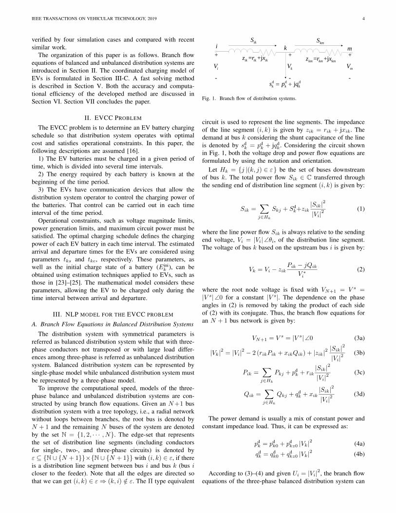
To improve the computational speed, models of the three-phase balance and unbalanced distribution systems are con-structed by using branch flow equations. Given an N+1 busdistribution system with a tree topology, i.e., a radial networkwithout loops between branches, the root bus is denoted byN + 1 and the remaining N buses of the system are denotedby the set N = 1, 2, · · · , N. The edge-set that representsthe set of distribution line segments (including conductorsfor single-, two-, and three-phase circuits) is denoted byε ⊆ N ∪ N + 1×N ∪ N + 1 with (i, k) ∈ ε, if thereis a distribution line segment between bus i and bus k (bus icloser to the feeder). Note that all the edges are directed sothat we can get (i, k) ∈ ε⇒ (k, i) /∈ ε. The Π type equivalent

= +jik ik ikz r x = +jkm km kmz r x

i k mikS

kmS

d d djk k ks p q

+

-

iV

+

-

mV

+

-

kV

Fig. 1. Branch flow of distribution systems.

circuit is used to represent the line segments. The impedanceof the line segment (i, k) is given by zik = rik + jxik. Thedemand at bus k considering the shunt capacitance of the lineis denoted by sd

k = pdk + jqd

k. Considering the circuit shownin Fig. 1, both the voltage drop and power flow equations areformulated by using the notation and orientation.

Let Hk = j |(k, j) ∈ ε be the set of buses downstreamof bus k. The total power flow Sik ∈ C transferred throughthe sending end of distribution line segment (i, k) is given by:

Sik =∑j∈Hk

Skj + Sdk+zik

|Sik|2

|Vi|2(1)

where the line power flow Sik is always relative to the sendingend voltage, Vi = |Vi|∠θi, of the distribution line segment.The voltage of bus k based on the upstream bus i is given by:

Vk = Vi − zikPik − jQik

V ∗i(2)

where the root node voltage is fixed with VN+1 = V s =|V s|∠0 for a constant |V s|. The dependence on the phaseangles in (2) is removed by taking the product of each sideof (2) with its conjugate. Thus, the branch flow equations foran N + 1 bus network is given by:

VN+1 = V s = |V s|∠0 (3a)

|Vk|2 = |Vi|2 − 2 (rikPik + xikQik) + |zik|2|Sik|2

|Vi|2(3b)

Pik =∑j∈Hk

Pkj + pdk + rik

|Sik|2

|Vi|2(3c)

Qik =∑j∈Hk

Qkj + qdk + xik

|Sik|2

|Vi|2(3d)

The power demand is usually a mix of constant power andconstant impedance load. Thus, it can be expressed as:

pdk = pd

k0 + pdkz0 |Vk|

2 (4a)

qdk = qd

k0 + qdkz0 |Vk|

2 (4b)

According to (3)–(4) and given Ui = |Vi|2, the branch flowequations of the three-phase balanced distribution system can

IEEE TRANSACTIONS ON VEHICULAR TECHNOLOGY, 2019 5

be simplified as:

UN+1 = |V s|2 = Us (5a)Uk = Ui − 2 (rikPik + xikQik) + cvik (P,Q) , k ∈ N (5b)

Pik =∑j∈Hk

Pkj + pdk + cpik (P,Q), k ∈ N (5c)

Qik =∑j∈Hk

Qkj + qdk + cqik (P,Q), k ∈ N (5d)

pdk = pd

k0 + pdkz0Uk, k ∈ N (5e)

qdk = qd

k0 + qdkz0Uk, k ∈ N (5f)

where cvik (P,Q) = |zik|2|Sik|2/|Vi|2, cpik (P,Q) =

rik|Sik|2/|Vi|2, and cqik (P,Q) = xik|Sik|2

/|Vi|2.

B. Branch Flow in Unbalanced Distribution Systems

In the actual distribution system, the overhead lines areusually not transposed. Thus, the off diagonal elements ofthe line mutual impedance matrix are not equal any more.Moreover, the three-phase loads connected to each node areusually not equal. As a result, the three-phase parameters of thedistribution system are asymmetrical. For each line segment(i, k) ∈ ε, the voltage equation is given by:

V k = V i − zik [(P ik − jQik)∅V ∗i ] (6)

where zik ∈ C3×3, V k = [Vka, Vkb, Vkc]T, V i =

[Via, Vib, Vic]T, P ik = [Pika, Pikb, Pikc]

T, and Qik =[Qika, Qikb, Qikc]

T. The symbol of ∅ denotes the element-wise division.

Unlike the per-phase equivalent case, both sides of (6)cannot remove the dependence on phase angles by multiplyingthe complex conjugate. This is due to the fact that there is acoupling between phases that arises from the cross-product ofthe three-phase equation for the phase voltage and line current.To address this problem, it can be observed that voltagemagnitudes between phases are similar, i.e., |Via| ≈ |Vib| ≈|Vic| [26] and the unbalance on each phase are not that severe.Thus, voltage magnitudes are assumed to be approximatelyequal. The unbalance of the three-phase angle α is relativelysmall (typically within 1 ∼ 3). Thus, we ignore α andassume that the three-phase voltage at each node is equal.By multiplying both sides of (6) with its conjugate vector, thevoltage equation in (5b) can be updated as:

|V k|2 = |V i|2 − 2 (rikPik + xikQik) + cuik (P ,Q) , k ∈ N(7)

a =[1 e−j2π/3ej2π/3

]T(8)

rik = ReaaH rik + Im

aaH xik (9)

xik = ReaaH xik − Im

aaH rik (10)

cuik (P ,Q) = [zik (S∗ik∅V ∗i )] [z∗ik (Sik∅V i)] (11)

where the symbol of denotes the element-wise multiplica-tion.

We assume that the three-phase voltages magnitudes ofeach node are equal in order to obtain a constant equivalentresistance matrix rik and reactance matrix xik, thus simpli-fying the voltage equation. This hypothesis is only used toderive Eq. (7) and is not used for other purposes. Eq. (7)shows that when the three-phase power of each branch isunequal, the three-phase voltages magnitudes of each nodeare unequal as well. Thus, Eq. (7) simulates the three-phaseunbalanced distribution network. Eq. (7) has high accuracy,because the unbalance of three-phase voltage of each nodein the actual distribution network is very small. The voltageimbalance limit in the distribution system is that the negativesequence voltage divided by the positive sequence voltagemust be below 2% which is required by the National ElectricalManufacturers Association (NEMA). In the actual distributionnetwork, the imbalance of three-phase voltage is very smallwhile the imbalance of three-phase power may be large.

Branch flow equations in (5c) and (5d) can be updated as:

P ik =∑j∈Hk

P kj + pdk + cpik (P ,Q), k ∈ N (12)

Qik =∑j∈Hk

Qkj + qdk + cqik (P ,Q), k ∈ N (13)

where cpik (P ,Q) = Re (Sik∅V i) (V i − V k),cqik (P ,Q) = Im (Sik∅V i) (V i − V k)

Power demand equations in (5e) and (5f) can be updatedas:

pdk = pd

k0 + pdkz0Uk, k ∈ N (14)

qdk = qd

k0 + qdkz0Uk, k ∈ N (15)

The three-phase voltage of the root node in (5a) is updatedas:

UN+1 = |V s| |V s| (16)

C. Model for EVCC

The objective function for the coordinated charging modelof EVs is to minimize the total charging costs of holders, givenby:

J = min

tmax∑t=t1

ρ (t)

(K∑k=1

PEVk,t +

M∑m=1

PEVm,β,t

)∆t (17)

Constraints on the charging power of each EV with thethree-phase charging mode are formulated by:

0 ≤ PEVk,t ≤ PEVk,max (18)

PEVk,a,t = PEVk,b,t = PEVk,c,t =PEVk,t

3(19)

The constraint on the charging power of each EV with thesingle-phase charging mode is formulated by:

0 ≤ PEVm,β,t ≤ PEVm,max (20)

IEEE TRANSACTIONS ON VEHICULAR TECHNOLOGY, 2019 6

Constraints on the power demand of each EV with the three-and single-phase charging modes are given by:

η

tke∑t=tks

PEVk,t∆t = Ecapk − E

inik (21)

η

tme∑t=tms

PEVm,β,t∆t = Ecapm − Eini

m (22)

The rates of charging power constraints are consideredin Eqs. (18)–(20), while the SOC constraints are indirectlyconsidered in Eqs. (21) and (22). The discharging mode(Vehicle to Grid) can be added to this work as well. To dothis, it is only needed to modify Eqs. (18)–(22). However,since the discharging mode can reduce the battery life span,it is not considered in this paper.

The constraint on the nodal voltage of the distributionsystem is given by:

Umin ≤ Un,α,t ≤ Umax (23)

The constraint on the thermal loading of each line is givenby:

0 ≤ Pik,α,t ≤ Pmaxik,α,t (24)

The constraint on the thermal loading of each transformeris given by:

0 ≤ PT,α,t ≤ PmaxT,α,t (25)

For the balanced distribution system, the objective functionis formulated in (17). Equality constraints are formulatedin (5a)–(5f), (19), and (21). Inequality constraints are formu-lated in (20) and (23)–(25). For the unbalanced distributionsystem, the objective function is formulated in (17). Equalityconstraints are formulated in (7), (12)–(16), (19), and (21)–(22). Inequality constraints are formulated in (18), (20)and (23)–(25).

The charging power of EVs is constrained by the voltagemagnitude and branch power. For different distribution net-work models, the function relationship between the voltagemagnitude, branch power, and charging power is different,which leads to different objective function values, i.e., totalcharging costs of holders. If the distribution network is bal-anced and all EVs are charged with the three–phase mode, thebalanced distribution network model can be used. Otherwise,the unbalanced distribution network model must be adopted.

IV. LP MODEL FOR THE EVCC PROBLEM

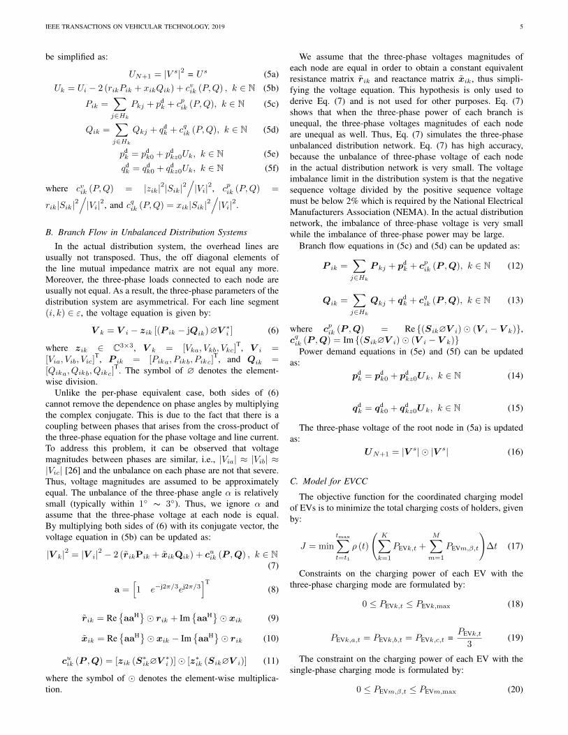
In the formulated NLP EVCC problem, only the model ofdistribution network is nonlinear, while other parts are linear.We propose a method to linearize the model of balancedand unbalanced distribution network. However, for the chargescheduling problem, the initial point of linearizing is unknownin advance. We propose a method to calculate the initial pointof linearizing. The linearizing process is closely associatedwith the charging scheduling model.

The advantage of LP is that it can be solved quickly byusing sophisticated solver. A mixed-integer LP is formulatedin [16]. However, polar coordinate power flow equations areadopted. While in our paper, branch power flow equations are

utilized. The variable number is much less than that in [16].Further, non-linear inequalities are linearized by introducingnew auxiliary variables in [16]. As a result, variables havesharply increased. While in our paper, we linearize the non-linear terms in branch power flow equations by using Taylorexpansion and the variable number keeps constant.

A. Linearization of Branch Flow Equations in the BalancedDistribution System

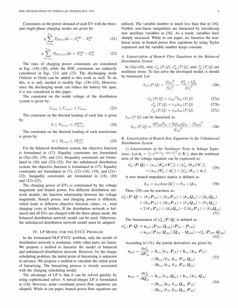
In (5a)–(5f), only cvik (P,Q), cpik (P,Q), and cqik (P,Q) arenonlinear terms. To fast solve the developed model, it shouldbe linearized. Let:

hik (P,Q) =|Sik|2

|Vi|2=P 2ik +Q2

ik

|Vi|2(26)

cvik (P,Q) = |zik|2hik (P,Q) (27a)cpik (P,Q) = rikhik (P,Q) (27b)cqik (P,Q) = xikhik (P,Q) (27c)

hik (P,Q) can be linearized as:

hik (P,Q) ≈ 2Pik0Pik + 2Qik0Qik − |Sik0|2

|Vi0|2(28)

B. Linearization of Branch flow Equations in the UnbalancedDistribution System

1) Linearization of the Nonlinear Term in Voltage Equa-tions: Let ai =

[1, ej2π/3e−j2π/3

]T ∅ |V i|, then the nonlinearterm of the voltage equation can be expressed as:

cuik (P ,Q) = [zik (S∗ik∅V ∗i )] [z∗ik (Sik∅V i)]

≈ [zik (S∗ik a∗i )] [z∗ik (Sik ai)](29)

A new branch impedance matrix is defined as:

zik = zikdiag (a∗i ) = rik + jxik (30)

Then, (29) can be rewritten as:

cuik (P ,Q) = (rikP ik) (rikP ik) + (xikQik) (xikQik)

+ (xikP ik) (xikP ik) + (rikQik) (rikQik)

+ 2 (rikP ik) (xikQik)−2 (xikP ik) (rikQik)(31)

The linearization of cuik (P ,Q) is defined as:

cuik (P ,Q) ≈ upik (P ik0,Qik0) (P ik − P ik0)

+ uqik (P ik0,Qik0) (Qik −Qik0) + cuik (P ik0,Qik0)(32)

According to (31), the partial derivatives are given by:

upik =∂cuik∂P ik

= hxx (rik,P ik) + hxx (xik,P ik)

+ 2hxy (rik, xik,P ik,Qik)

− 2hxy (xik, rik,P ik,Qik)

(33)

uqik =∂cuik∂Qik

= hxx (rik,Qik) + hxx (xik,Qik)

+ 2hxy (xik, rik,Qik,P ik)

− 2hxy (rik, xik,Qik,P ik)

(34)

IEEE TRANSACTIONS ON VEHICULAR TECHNOLOGY, 2019 7

where functions hxx and hxy are respectively given by:

hxx (A,x) = 2diag (Ax) A (35)

hxy (A,B,x,y) = diag (By) A (36)

2) Linearization of the Nonlinear Term in Power Equations:The power loss across line segment (i, k) is given by:

Slik = (Sik∅V i) [zik (S∗ik∅V ∗i )] (37)

Another branch impedance matrix is redefined as:

zik = rik + jxik = zik (aia

Hi

)(38)

According to (38), by separating the real part from theimaginary one, it can be obtained:

rik = Reaia

Hi

rik − Im

aia

Hi

xik (39)

xik = Reaia

Hi

xik + Im

aia

Hi

rik (40)

For the sake of simplicity, (37) can be rewritten as:

Slik = (P ik + jQik) [zik (P ik − jQik)] (41)

According to (39)–(41), by separating the active power fromthe reactive power, it can be obtained:

cpik (P ,Q) = real(Slik

)= P ik (rikP ik + xikQik)

+ Qik (rikQik − xikP ik)(42)

cqik (P ,Q)= imag(Slik

)=P ik (xikP ik − rikQik)

+ Qik (rikP ik + xikQik)(43)

The linearization of cpik (P ,Q) and cqik (P ,Q) are respec-tively defined as:

cpik (P,Q)≈fpik (P ik0,Qik0) (P ik − P ik0)

+f qik (P ik0,Qik0) (Qik−Qik0)+cpik (P ik0,Qik0)(44)

cqik (P,Q)≈gpik (P ik0,Qik0) (P ik − P ik0)

+gqik (P ik0,Qik0) (Qik−Qik0)+cqik (P ik0,Qik0)(45)

Partial derivative terms in (44) and (45) are respectivelygiven by:

fpik =∂cpik∂P ik

= hxx (rik,P ik) + hxy (xik,P ik,Qik)

− hyx (xik,Qik,P ik)

(46)

f qik =∂cpik∂Qik

= hxx (rik,Qik)− hxy (xik,Qik,P ik)

+ hxy (xik,P ik,Qik)

(47)

gpik =∂cqik∂P ik

= hxx (xik,P ik)− hxy (rik,P ik,Qik)

+ hyx (rik,Qik,P ik)

(48)

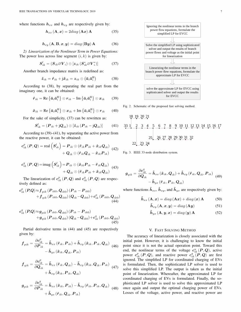
Ignoring the nonlinear terms in the branch

power flow equations, formulate the

simplified LP for EVCC

Solve the simplified LP using sophisticated

solver and output the results of branch

power flows and voltage as the initial point

for linearization

Linearizing the nonlinear terms in the

branch power flow equations, formulate the

approximate LP for EVCC

solve the approximate LP for EVCC using

sophisticated solver and output the results

for EVCC

Fig. 2. Schematic of the proposed fast solving method.

33 1 2 3 4 5 6 7 8 9 10 11 12 13 14 15 16

18 19 20 21

17

22 23 24

25 26 27 28 29 30 31 32

Fig. 3. IEEE 33-node distribution system.

gqik =∂cqik∂Qik

= hxx (xik,Qik) + hxy (rik,Qik,P ik)

− hyx (rik,P ik,Qik)

(49)

where functions hxx, hxy , and hyx are respectively given by:

hxx (A,x) = diag (Ax) + diag (x) A (50)

hxy (A,x,y) = diag (Ay) (51)

hyx (A,y,x) = diag (y) A (52)

V. FAST SOLVING METHOD

The accuracy of linearization is closely associated with theinitial point. However, it is challenging to know the initialpoint since it is not the actual operation point. Toward thisend, the nonlinear terms of the voltage cuik (P ,Q), activepower cpik (P ,Q), and reactive power cqik (P ,Q) are firstignored. The simplified LP for coordinated charging of EVsis formulated. Then, the sophisticated LP solver is used tosolve this simplified LP. The output is taken as the initialpoint of linearization. Whereafter, the approximated LP forcoordinated charging of EVs is formulated. Finally, the so-phisticated LP solver is used to solve this approximated LPonce again and output the optimal charging power of EVs.Losses of the voltage, active power, and reactive power are

IEEE TRANSACTIONS ON VEHICULAR TECHNOLOGY, 2019 8

much less than the corresponding linear terms in branch flowequations. In addition, the linearization is performed at theinitial point that is the result of the simplified linear model.Thus, the deviation is relatively small. That is, the accuracyof the proposed linearization strategy can be guaranteed. Thecomputational speed of the proposed method can also beguaranteed since both formulated models belong to the LPproblem. A schematic diagram of the proposed fast solvingmethod is shown in Fig. 2.

VI. CASE STUDIES

In the simulation cases, noon or night are chosen as thecharging periods since these time periods are in coincidencewith the charging habits of most EV holders.

A. Case 1

1) Simulation Conditions: Fig. 3 shows the IEEE 33-nodemedium voltage (MV) distribution system to test the capabilityof the proposed method. The impedance matrix of transmissionlines is shown in Table I. In this system, node 33 is taken asthe slack node and its voltage is kept to be 1.00 p.u.. The restof nodes are taken as PQ nodes. The base conventional load ateach node is shown in Table II. The constant power load modelis deployed. There are four parking lots of EVs connected atnodes 17, 21, 24, and 32, respectively. There are 40 EVs ineach parking lot. The single-phase base power and voltageare chosen to be 1000/3 kVA and 12.66/

√3 kV, respectively.

The back forward sweep method is used to calculate the powerflow.

Other simulation conditions are set as follows:1) All EV owners are willing to participate in the coordi-

nated charging. The charging power of each EV is fully con-trollable. The charging time period is between 12:00∼14:00.

2) The conventional load at each node is equal to the baseload between 12:00∼13:00 and that of 80% base load between13:00∼14:00. The power factor is 0.95.

3) The power prices in the time range of 12:00∼13:00 and13:00∼14:00 are 0.8 and 0.4 Yuan/kWh, respectively.

4) All EVs adopt the three-phase charging mode.5) The charging demand of each EV is 10 kWh.6) Minimal and maximal charging power of each EV are 0

and 10 kW, respectively.7) The charging efficiency is set to be 1.0.8) The optimization time interval is 1 hour.9) The upper and lower voltage limits are 1.0 and 0.9 p.u.,

respectively.2) Simulation Results: All the programs are written with

MATLAB. The LP is solved by using the library functionlinprog. The precise model is solved by the primal dual interiorpoint method [27]. The CPU of the computer is Intel (R) Core(TM) i3-4510. The main frequency of the CPU is 3.5 GHzwith 32G RAM.

Some results are shown in Table III and Table IV, where f.0and f.1 represent the optimization results during 12:00∼13:00and 13:00∼14:00 solved by the simplified LP, respectively.PM.0 and PM.1 represent the optimization results during12:00∼13:00 and 13:00∼14:00 solved by the approximate

TABLE ILINE IMPEDANCE OF IEEE 33-NODE DISTRIBUTION NETWORK

Line i∼jZaa

(Ω)Zbb

(Ω)Zcc

(Ω)Zab

(Ω)Zac

(Ω)Zbc

(Ω)

33∼1 Real 0.0935 0.0933 0.0931 0.0009 0.0013 0.0011Imag 0.0477 0.0475 0.0474 0.0004 0.0007 0.0005

1∼2 Real 0.5003 0.4989 0.4979 0.0049 0.0073 0.0059Imag 0.2548 0.2541 0.2536 0.0025 0.0037 0.0030

2∼3 Real 0.3714 0.3704 0.3696 0.0036 0.0054 0.0043Imag 0.1891 0.1886 0.1882 0.0018 0.0027 0.0022

3∼4 Real 0.3868 0.3856 0.3849 0.0038 0.0057 0.0045Imag 0.1970 0.1964 0.1960 0.0019 0.0029 0.0023

4∼5 Real 0.8312 0.8288 0.8271 0.0081 0.0122 0.0098Imag 0.7176 0.7154 0.7140 0.0070 0.0106 0.0084

5∼6 Real 0.1900 0.1894 0.1890 0.0018 0.0028 0.0022Imag 0.6280 0.6262 0.6249 0.0061 0.0092 0.0074

6∼7 Real 0.7220 0.7199 0.7185 0.0071 0.0106 0.0085Imag 0.2386 0.2379 0.2374 0.0023 0.0035 0.0028

7∼8 Real 1.0454 1.0423 1.0403 0.0103 0.0154 0.0123Imag 0.7510 0.7488 0.7473 0.0074 0.0110 0.0088

8∼9 Real 1.0596 1.0565 1.0544 0.0104 0.0156 0.0125Imag 0.7510 0.7488 0.7473 0.0074 0.0110 0.0088

9∼10 Real 0.1995 0.1989 0.1985 0.0019 0.0029 0.0023Imag 0.0659 0.0657 0.0656 0.0006 0.0009 0.0007

10∼11 Real 0.3800 0.3788 0.3781 0.0037 0.0056 0.0044Imag 0.1256 0.1252 0.1250 0.0012 0.0018 0.0014

11∼12 Real 1.4900 1.4856 1.4826 0.0146 0.0220 0.0176Imag 1.1723 1.1688 1.1665 0.0115 0.0173 0.0138

12∼13 Real 0.5497 0.5480 0.5470 0.0054 0.0081 0.0064Imag 0.7235 0.7214 0.7200 0.0071 0.0106 0.0085

13∼14 Real 0.5998 0.5980 0.5969 0.0059 0.0088 0.0070Imag 0.5338 0.5323 0.5312 0.0052 0.0078 0.0063

14∼15 Real 0.7514 0.7491 0.7477 0.0074 0.0111 0.0088Imag 0.5531 0.5515 0.5544 0.0054 0.0081 0.0065

15∼16 Real 1.3083 1.3044 1.3018 0.0128 0.0193 0.0154Imag 1.7468 1.7416 1.7382 0.0172 0.0258 0.0206

16∼17 Real 0.7429 0.7407 0.7393 0.0073 0.0109 0.0087Imag 0.5826 0.5808 0.5797 0.0057 0.0086 0.0068

17∼18 Real 0.1664 0.1659 0.1656 0.0016 0.0024 0.0019Imag 0.1588 0.1583 0.1580 0.0015 0.0023 0.0018

18∼19 Real 1.5267 1.5222 1.5192 0.0150 0.0225 0.0180Imag 1.3757 1.3716 1.3689 0.0135 0.0203 0.0162

19∼20 Real 0.4156 0.4144 0.4135 0.0040 0.0061 0.0049Imag 0.4855 0.4841 0.4831 0.0047 0.0071 0.0057

20∼21 Real 0.7195 0.7174 0.7159 0.0070 0.0106 0.0085Imag 0.9513 0.9485 0.9466 0.0093 0.0140 0.0112

21∼22 Real 0.4579 0.4566 0.4557 0.0045 0.0067 0.0054Imag 0.3129 0.3119 0.3113 0.0030 0.0046 0.0036

22∼23 Real 0.9114 0.9087 0.9069 0.0089 0.0134 0.0107Imag 0.7197 0.7176 0.7161 0.0070 0.0106 0.0085

23∼24 Real 0.9094 0.9067 0.9049 0.0089 0.0134 0.0107Imag 0.7116 0.7095 0.7081 0.0070 0.0105 0.0084

24∼25 Real 0.2060 0.2054 0.2050 0.0020 0.0030 0.0024Imag 0.1049 0.1046 0.1044 0.0010 0.0015 0.1044

25∼26 Real 0.2884 0.2876 0.2870 0.0028 0.0042 0.0034Imag 0.1468 0.1464 0.1461 0.0014 0.0021 0.0017

26∼27 Real 1.0748 1.0717 1.0695 0.0105 0.0158 0.0127Imag 0.9477 0.9449 0.9430 0.0093 0.0140 0.0112

27∼28 Real 0.8162 0.8138 0.8122 0.0080 0.0120 0.0096Imag 0.7111 0.7090 0.7076 0.0070 0.0105 0.0084

28∼29 Real 0.5151 0.5135 0.5125 0.0050 0.0076 0.0060Imag 0.2623 0.2616 0.2610 0.0025 0.0038 0.0031

29∼30 Real 0.9890 0.9860 0.9841 0.0097 0.0146 0.0116Imag 0.9774 0.9745 0.9726 0.0096 0.0144 0.0115

30∼31 Real 0.3151 0.3142 0.3136 0.0031 0.0046 0.0037Imag 0.3637 0.3662 0.3655 0.0036 0.0054 0.0043

31∼32 Real 0.3461 0.3450 0.3444 0.0034 0.0051 0.0040Imag 0.5381 0.5365 0.5355 0.0053 0.0079 0.0063

LP, respectively. PD.0 and PD.1 represent the optimizationresults during 12:00∼13:00 and 13:00∼14:00 solved by theprecise nonlinear model, respectively. Pf.0 and Pf.1 represent

IEEE TRANSACTIONS ON VEHICULAR TECHNOLOGY, 2019 9

TABLE IILOAD OF IEEE 33-NODE DISTRIBUTION SYSTEM

Node Phase A [kW] Phase B [kW] Phase C [kW]1 32 + 19i 33 + 20i 35 + 21i2 30 + 13i 31 + 15i 29 + 13i3 45 + 30i 0 + 0i 35 + 24i4 20 + 10i 20 + 10i 20 + 10i5 20 + 6i 20 + 7i 20 + 7i6 65 + 33i 70 + 34i 65 + 33i7 70 + 34i 65 + 33i 65 + 33i8 20 + 7i 18 + 6i 22 + 7i9 21 + 7i 20 + 7i 0+ 0i

10 14 + 9i 16 + 11i 15 + 10i11 20 + 11i 20 + 12i 20 + 12i12 21 + 12i 19 + 11i 20 + 12i13 40 + 28i 38 + 27i 42 + 25i14 0 + 0i 19 + 3i 20 + 3i15 19 + 6i 20 + 7i 21 + 7i16 19 + 6i 21 + 7i 20 + 7i17 30 + 14i 30 + 13i 30 + 13i18 33 + 15i 29 + 13i 28 + 12i19 29 + 13i 28 + 12i 33 + 15i20 29 + 12i 30 + 13i 31 + 15i21 28 + 12i 33 + 15i 29 + 13i22 30 + 16i 31 + 17i 29 + 17i23 130 + 60i 140+ 70i 150+ 70i24 150+ 70i 130+ 70i 140+ 60i25 20 + 8i 20 + 8i 20 + 9i26 18 + 7i 22 + 9i 20 + 9i27 19 + 6i 22 + 8i 19 + 6i28 38 + 23i 42 + 25i 40 + 22i29 60 + 180i 70 + 210i 70 + 210i30 45 + 20i 51 + 23i 54 + 27i31 70 + 33i 72 + 35i 68 + 32i32 20 + 13i 20 + 14i 20 + 13i

TABLE IIIOPTIMAL CHARGING POWER FOR DIFFERENT METHODS IN CASE 1

Nodes 17 21 24. 32 ComputationalTime [s]

f.0 [kW] 56.8 0 0 0 0.130f.1 [kW] 343.2 400 400 400PM.0 [kW] 111 0 0 0 0.198PM.1 [kW] 289 400 400 400PD.0 [kW] 111.4 0 0 0 8.295PD.1 [kW] 288.6 400 400 400

voltages of power flow calculations during 12:00∼13:00 and13:00∼14:00, by substituting the optimal charging power ofEVs using the simplified LP into the precise power flow equa-tions, respectively. PF.0 and PF.1 represent voltages of powerflow calculations during 12:00∼13:00 and 13:00∼14:00, bysubstituting the optimal charging power of EVs using theapproximate LP into the precise power flow equations, respec-tively.

As can be seen in Table III and Table IV, the resultsobtained by the simplified and approximate LP are relativelyclose. Thus, the result is of high precision via the initial pointobtained by the simplified LP for linearizing the nonlinearterms of branch flow equations. Moreover, the optimizationresults obtained by the approximate LP are very close to thoseof the primal dual interior point method. This observationdemonstrates that the proposed method has a high precision.However, the computational speed of the proposed method isabout 40 times higher than that of the primal dual interiorpoint method. As can be seen from the results of power flow

TABLE IVOPTIMAL VOLTAGES FOR DIFFERENT METHODS IN CASE 1

Nodes 17 21 24 32

f.0 [p.u.]0.9168 0.9921 0.9704 0.92290.9120 0.9917 0.9707 0.91720.9137 0.9916 0.9702 0.9195

f.1 [p.u.]0.9041 0.9858 0.9663 0.91480.9000 0.9854 0.9665 0.90990.9016 0.9854 0.9661 0.9124

PM.0 [p.u.]0.9099 0.9919 0.9693 0.91940.9044 0.9914 0.9695 0.91310.9064 0.9914 0.9690 0.9158

PM.1 [p.u.]0.9045 0.9855 0.9653 0.91220.9000 0.9851 0.9655 0.90690.9017 0.9851 0.9651 0.9096

PD.0 [p.u.]0.9098 0.9919 0.9693 0.91940.9043 0.9914 0.9695 0.91310.9063 0.9914 0.9690 0.9157

PD.1 [p.u.]0.9045 0.9856 0.9654 0.91220.9000 0.9851 0.9655 0.90690.9017 0.9851 0.9651 0.9096

Pf.0 [p.u.]0.9142 0.9919 0.9695 0.92030.9087 0.9915 0.9697 0.91400.9107 0.9914 0.9692 0.9167

Pf.1 [p.u.]0.9000 0.9855 0.9651 0.91130.8954 0.9851 0.9653 0.90590.8971 0.9851 0.9649 0.9086

PF.0 [p.u.]0.9098 0.9919 0.9693 0.91940.9043 0.9914 0.9695 0.91310.9063 0.9914 0.9690 0.9157

PF.1 [p.u.]0.9045 0.9856 0.9654 0.91220.9000 0.9851 0.9655 0.90680.9017 0.9851 0.9651 0.9096

calculation in Table IV, the optimal charging power obtainedby the simplified LP may result in voltages dropping out of thelower limit (see the bold font). However, for the approximateLP, voltage results of the power flow calculation are very closeto those of the optimization results. Furthermore, all of thevoltages are within the rated range.

B. Case 2

1) Simulation Conditions: In this case, all the EVs areassumed to adopt the single-phase charging mode to testify thecapabilities of the proposed method. The simulation platformis the same as that of case 2 in [28]. Time-of-use electricityprices are set as 0.8, 0.4 Yuan/kWh during 12:00∼13:00and 13:00∼14:00, respectively. The conventional householdloads at each node of each phase are 4.5 and 3.6 kW during12:00∼13:00 and 13:00∼14:00, respectively. The chargingdemand of each EV is 5 kWh. The maximum charging poweris 4 kW. Other simulation conditions are set as same as thoseof case 2 in [28].

2) Simulation Results: All the programs are written withMATLAB. The simplified and approximate LP is solved usinglibrary function linprog. The precise model is solved bythe primal dual interior point method [27]. The computerconfiguration is the same as that in case 1. Simulation resultsof different optimization algorithms are shown in Table Vand Table VI. It can be seen that results of the proposedmethod are in good agreement with those of the primal dualinterior point method. However, the computational speed issignificantly superior to the primal dual interior point method.

IEEE TRANSACTIONS ON VEHICULAR TECHNOLOGY, 2019 10

TABLE VOPTIMAL CHARGING POWER FOR DIFFERENT METHODS IN CASE 2

Nodes 6 7 11 12 ComputationalTime [s]

f.0 [p.u.] 0.0188 0.0188 0.0188 0.0188 0.103f.1 [p.u.] 0.0750 0.0750 0.0750 0.0750PM.0 [p.u.] 0.0188 0.0188 0.0188 0.0188 0.161PM.1 [p.u.] 0.0750 0.0750 0.0750 0.0750PD.0 [p.u.] 0.0188 0.0188 0.0188 0.0188 1.390PD.1 [p.u.] 0.0750 0.0750 0.0750 0.0750

TABLE VIOPTIMAL VOLTAGE FOR DIFFERENT METHODS IN CASE 2

Nodes 6 7 11 12

f.0 [p.u.]0.9285 0.9358 0.9338 0.93480.9378 0.9428 0.9429 0.94040.9334 0.9429 0.9396 0.9418

f.1 [p.u.]0.9187 0.9260 0.9231 0.92630.9554 0.9539 0.9595 0.94890.9382 0.9543 0.9464 0.9545

PM.0 [p.u.]0.9216 0.9290 0.9270 0.92800.9322 0.9373 0.9375 0.93490.9275 0.9371 0.9338 0.9360

PM.1 [p.u.]0.9093 0.9167 0.9138 0.91710.9516 0.9501 0.9557 0.94480.9329 0.9493 0.9414 0.9495

PD.0 [p.u.]0.9209 0.9284 0.9263 0.92730.9317 0.9368 0.9370 0.93440.9271 0.9367 0.9334 0.9357

PD.1 [p.u.]0.9082 0.9157 0.9128 0.91600.9512 0.9497 0.9553 0.94440.9331 0.9494 0.9415 0.9496

PF.0 [p.u.]0.9215 0.9289 0.9269 0.92780.9318 0.9370 0.9370 0.93460.9274 0.9369 0.9337 0.9358

PF.1 [p.u.]0.9082 0.9157 0.9128 0.91600.9512 0.9497 0.9553 0.94440.9331 0.9494 0.9415 0.9496

C. Case 3

1) Simulation Conditions: In this case, the coexistence ofthe single- and three-phase charging modes for EVs in thedistribution system to test the capabilities of the proposedmethod. Simulation conditions are the same as those in case 2except that EVs connected to nodes 3, 4, 5, 8, 9, and 10 adoptthe three-phase charging mode and the maximum chargingpower of each EV is 12 kW.

2) Simulation Results: The optimal charging power of EVsat different nodes with different algorithms and the computa-tional time of the program are shown in Table VII. As can beseen, the computational efficiency of the proposed method isslightly better than that of case 2. This is because we choosethe total power rather than the single-phase charging powerfor EV with the three-phase charging mode as the optimizationvariable. The charging power of each phase is one-third of thisvariable. That is, with some simple mathematical techniques,the number of optimization variables, equality and inequalityconstraints can be the same as those in case 2. The imbalanceof the distribution system is reduced compared with that ofcase 2 due to the existence of three-phase charging mode.Thus, the numerical stability of the program is improved andthe computational speed is slightly higher than that of case 2.The voltage results using different optimization algorithms are

TABLE VIIOPTIMAL CHARGING POWER FOR DIFFERENT METHODS WITH SINGLE-

AND THREE-PHASE CHARGING COEXISTING

Nodes 5 6 10 11 ComputationalTime [s]

f.0 [p.u.] 0.0000 0.0188 0.0000 0.0188 0.093f.1 [p.u.] 0.0939 0.0750 0.0939 0.0750PM.0 [p.u.] 0.0000 0.0188 0.0000 0.0188 0.150PM.1 [p.u.] 0.0939 0.0750 0.0936 0.0750PD.0 [p.u.] 0.0000 0.0188 0.0000 0.0188 1.397PD.1 [p.u.] 0.0936 0.0750 0.0936 0.0750

1 2 3

Number of Simulation Case

0

1

2

3

4

5

6

7

8

9

Com

puta

tional T

ime [s]

simplified linear programming

approximate linear programming

primal dual interior point programming

Fig. 4. Computational efficiency with different methods.

similar with those in Table VI. Based on simulation results,we can draw the same conclusions as case 2.

The computational time of aforementioned three cases withdifferent optimization methods are shown in Fig. 4. As canbe seen, the calculation efficiency of the proposed methodis significantly better than that of the primal dual interiorpoint method and slightly worse than that of the simplifiedLP. However, the precision is very close to the primal dualinterior point method.

D. Case 4

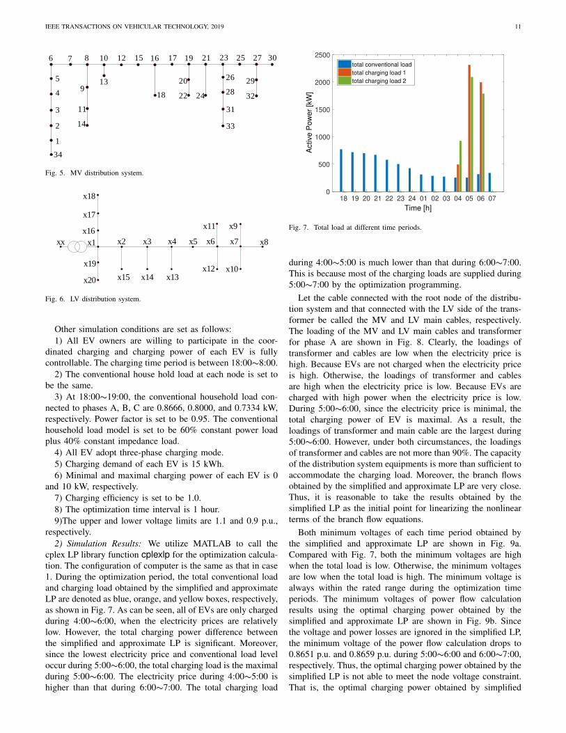
1) Simulation Conditions: A 354-node distribution systemis used to test the capabilities of the proposed method. Asshown in Fig. 5, the MV distribution system is a 34-nodedistribution system and the rated phase to ground voltage is13.8 kV. There are 16 low voltage (LV) distribution systems inthe simulation platform. The topology of each one is shown inFig. 6. The rated phase-to-ground voltage is 220 V. In Fig. 6,the capacity of the transformer is 250 kVA and the terminalnode ‘xx’ is connected to the MV distribution system at nodes11, 13, 14, 17, 18, 20, 22, 24-26, and 28-33, respectively. Therated currents of the cables in the MV and LV distributionnetworks are 200 A and 368 A, respectively. There is aconventional household load connected to each node in the LVdistribution system and each household has one EV connected.Node 34 is taken as the slack node and its voltage is kept tobe 1.1 p.u.. The rest of nodes are taken as PQ nodes. Thesingle-phase base power and voltages are chosen to be 1000kVA, 13.8 kV and 0.22 kV, respectively. The back forwardsweep method is used to calculate the power flow.

IEEE TRANSACTIONS ON VEHICULAR TECHNOLOGY, 2019 11

6 7 1210 17 19 23 25 27

13

15 16

18 24

21

20

22

8

11

14

9

26

31

33

28

34

1

2

4

3

5 29

32

30

Fig. 5. MV distribution system.

xx x3x2 x6 x7x4 x5x1

x19

x20

x8

x9

x10

x11

x12x13x14x15

x16

x17

x18

Fig. 6. LV distribution system.

Other simulation conditions are set as follows:1) All EV owners are willing to participate in the coor-

dinated charging and charging power of each EV is fullycontrollable. The charging time period is between 18:00∼8:00.

2) The conventional house hold load at each node is set tobe the same.

3) At 18:00∼19:00, the conventional household load con-nected to phases A, B, C are 0.8666, 0.8000, and 0.7334 kW,respectively. Power factor is set to be 0.95. The conventionalhousehold load model is set to be 60% constant power loadplus 40% constant impedance load.

4) All EV adopt three-phase charging mode.5) Charging demand of each EV is 15 kWh.6) Minimal and maximal charging power of each EV is 0

and 10 kW, respectively.7) Charging efficiency is set to be 1.0.8) The optimization time interval is 1 hour.9)The upper and lower voltage limits are 1.1 and 0.9 p.u.,

respectively.2) Simulation Results: We utilize MATLAB to call the

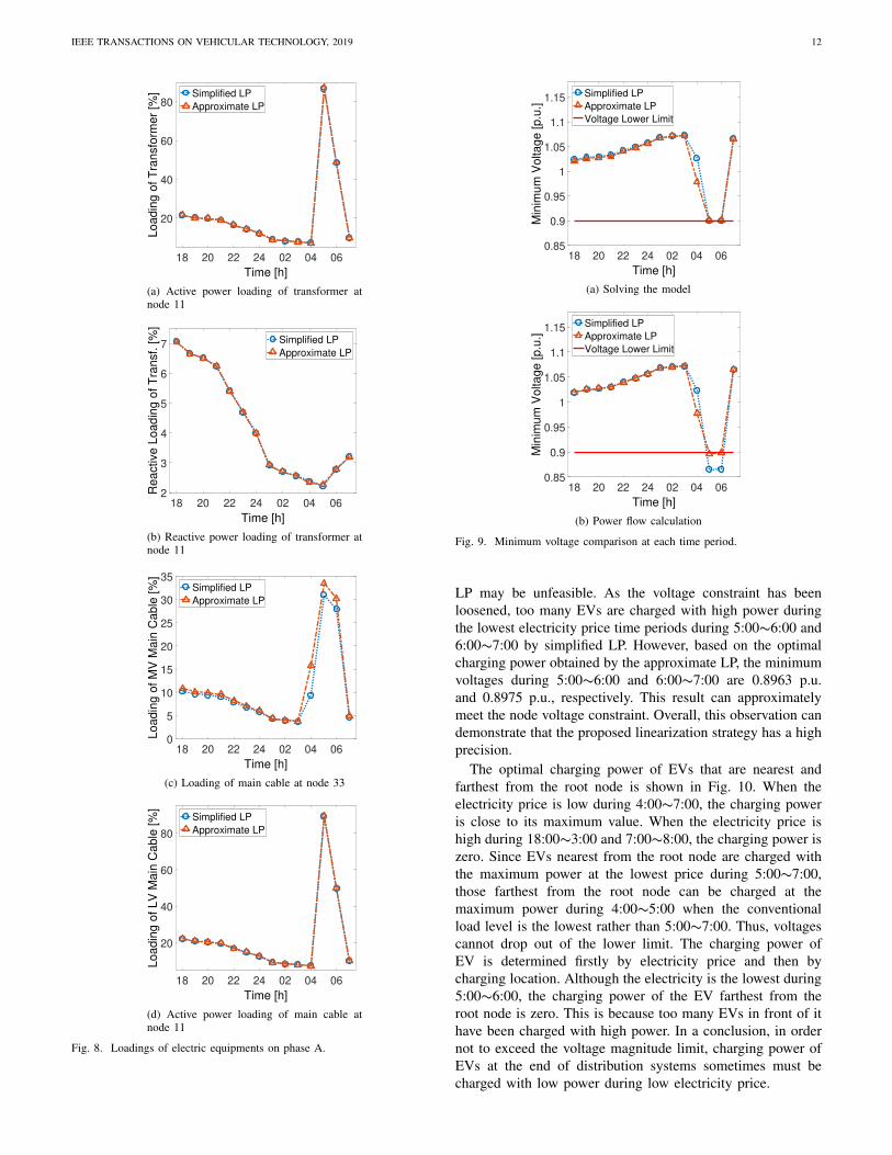
cplex LP library function cplexlp for the optimization calcula-tion. The configuration of computer is the same as that in case1. During the optimization period, the total conventional loadand charging load obtained by the simplified and approximateLP are denoted as blue, orange, and yellow boxes, respectively,as shown in Fig. 7. As can be seen, all of EVs are only chargedduring 4:00∼6:00, when the electricity prices are relativelylow. However, the total charging power difference betweenthe simplified and approximate LP is significant. Moreover,since the lowest electricity price and conventional load leveloccur during 5:00∼6:00, the total charging load is the maximalduring 5:00∼6:00. The electricity price during 4:00∼5:00 ishigher than that during 6:00∼7:00. The total charging load

18 19 20 21 22 23 24 01 02 03 04 05 06 07

Time [h]

0

500

1000

1500

2000

2500

Active

Po

we

r [k

W]

total conventional load

total charging load 1

total charging load 2

Fig. 7. Total load at different time periods.

during 4:00∼5:00 is much lower than that during 6:00∼7:00.This is because most of the charging loads are supplied during5:00∼7:00 by the optimization programming.

Let the cable connected with the root node of the distribu-tion system and that connected with the LV side of the trans-former be called the MV and LV main cables, respectively.The loading of the MV and LV main cables and transformerfor phase A are shown in Fig. 8. Clearly, the loadings oftransformer and cables are low when the electricity price ishigh. Because EVs are not charged when the electricity priceis high. Otherwise, the loadings of transformer and cablesare high when the electricity price is low. Because EVs arecharged with high power when the electricity price is low.During 5:00∼6:00, since the electricity price is minimal, thetotal charging power of EV is maximal. As a result, theloadings of transformer and main cable are the largest during5:00∼6:00. However, under both circumstances, the loadingsof transformer and cables are not more than 90%. The capacityof the distribution system equipments is more than sufficient toaccommodate the charging load. Moreover, the branch flowsobtained by the simplified and approximate LP are very close.Thus, it is reasonable to take the results obtained by thesimplified LP as the initial point for linearizing the nonlinearterms of the branch flow equations.

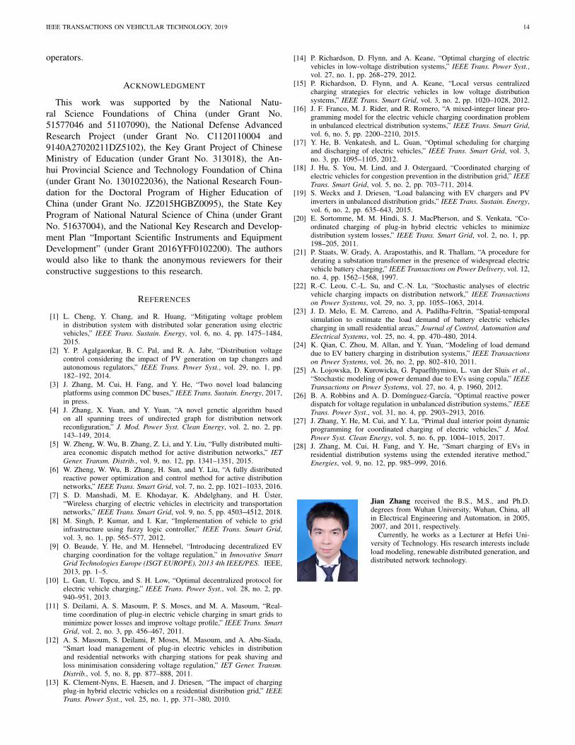
Both minimum voltages of each time period obtained bythe simplified and approximate LP are shown in Fig. 9a.Compared with Fig. 7, both the minimum voltages are highwhen the total load is low. Otherwise, the minimum voltagesare low when the total load is high. The minimum voltage isalways within the rated range during the optimization timeperiods. The minimum voltages of power flow calculationresults using the optimal charging power obtained by thesimplified and approximate LP are shown in Fig. 9b. Sincethe voltage and power losses are ignored in the simplified LP,the minimum voltage of the power flow calculation drops to0.8651 p.u. and 0.8659 p.u. during 5:00∼6:00 and 6:00∼7:00,respectively. Thus, the optimal charging power obtained by thesimplified LP is not able to meet the node voltage constraint.That is, the optimal charging power obtained by simplified

IEEE TRANSACTIONS ON VEHICULAR TECHNOLOGY, 2019 12

18 20 22 24 02 04 06

Time [h]

20

40

60

80

Lo

ad

ing

of

Tra

nsfo

rme

r [%

] Simplified LP

Approximate LP

(a) Active power loading of transformer atnode 11

18 20 22 24 02 04 06

Time [h]

2

3

4

5

6

7

Re

active L

oa

din

g o

f T

ransf.

[%

]

Simplified LP

Approximate LP

(b) Reactive power loading of transformer atnode 11

18 20 22 24 02 04 06

Time [h]

0

5

10

15

20

25

30

35

Loadin

g o

f M

V M

ain

Cable

[%

]

Simplified LP

Approximate LP

(c) Loading of main cable at node 33

18 20 22 24 02 04 06

Time [h]

20

40

60

80

Lo

ad

ing o

f L

V M

ain

Cab

le [

%]

Simplified LP

Approximate LP

(d) Active power loading of main cable atnode 11

Fig. 8. Loadings of electric equipments on phase A.

18 20 22 24 02 04 06

Time [h]

0.85

0.9

0.95

1

1.05

1.1

1.15

Min

imum

Voltage [p.u

.]

Simplified LP

Approximate LP

Voltage Lower Limit

(a) Solving the model

18 20 22 24 02 04 06

Time [h]

0.85

0.9

0.95

1

1.05

1.1

1.15

Min

imu

m V

olta

ge

[p

.u.]

Simplified LP

Approximate LP

Voltage Lower Limit

(b) Power flow calculation

Fig. 9. Minimum voltage comparison at each time period.

LP may be unfeasible. As the voltage constraint has beenloosened, too many EVs are charged with high power duringthe lowest electricity price time periods during 5:00∼6:00 and6:00∼7:00 by simplified LP. However, based on the optimalcharging power obtained by the approximate LP, the minimumvoltages during 5:00∼6:00 and 6:00∼7:00 are 0.8963 p.u.and 0.8975 p.u., respectively. This result can approximatelymeet the node voltage constraint. Overall, this observation candemonstrate that the proposed linearization strategy has a highprecision.

The optimal charging power of EVs that are nearest andfarthest from the root node is shown in Fig. 10. When theelectricity price is low during 4:00∼7:00, the charging poweris close to its maximum value. When the electricity price ishigh during 18:00∼3:00 and 7:00∼8:00, the charging power iszero. Since EVs nearest from the root node are charged withthe maximum power at the lowest price during 5:00∼7:00,those farthest from the root node can be charged at themaximum power during 4:00∼5:00 when the conventionalload level is the lowest rather than 5:00∼7:00. Thus, voltagescannot drop out of the lower limit. The charging power ofEV is determined firstly by electricity price and then bycharging location. Although the electricity is the lowest during5:00∼6:00, the charging power of the EV farthest from theroot node is zero. This is because too many EVs in front of ithave been charged with high power. In a conclusion, in ordernot to exceed the voltage magnitude limit, charging power ofEVs at the end of distribution systems sometimes must becharged with low power during low electricity price.

IEEE TRANSACTIONS ON VEHICULAR TECHNOLOGY, 2019 13

18 20 22 24 02 04 06

Time [h]

0

2

4

6

8

10

Charg

ing P

ow

er

[kW

]

Simplified LP

Approxiamate LP

(a) EV farthest from the root node

18 20 22 24 02 04 06

Time [h]

0

2

4

6

8

10

Charg

ing P

ow

er

[kW

]

Simplified LP

Approximate LP

(b) EV nearest from the root node

Fig. 10. Optimal charging power of EVs in the distribution system.

3) Comparison with Selected Method: As can be seen inFig. 7–Fig. 10, all the EVs are only charged during 4:00∼7:00and the charging power is zero during other time periods.Thus, for the third and forth steps in Fig. 2, the linearizationand optimization time periods can be reduced to 4:00∼7:00.Hence, the computational speed can be further improved. Theoptimization results of the proposed method are compared withthose in [16] and shown in Table VIII. As can be seen, thecomputational speed of the proposed method is much fasterthan that of [16]. This is because the model formulated in thispaper is based on the branch flow equation. The optimizationvariables do not contain the branch current and the phase angleof the node voltage. However, the model in [16] adopts thecurrent type power flow equation in the Cartesian coordinatesystem. Many variables and constraints are introduced to lin-earize the branch current constraint. The number of variablesin [16] is several times of the proposed model. The numberof branch current and node voltage constraints in [16] is morethan 10 times and 5 times of the proposed method. This resultsin a significant increase of the computational time. In addition,discrete variables are also introduced in [16] and makes themodel non-convex. Also, this can significantly increase thetotal computational time.

VII. CONCLUSIONS AND DISCUSSION

In this paper, branch flow equations of balanced and un-balanced distribution systems are derived. The model forcoordinated charging of EVs is proposed to minimize thetotal charging cost of holders. The charging demand, three-

TABLE VIIICOMPARISON WITH THE MODEL IN [16]

Metrics Methodin [16]

Proposed MethodSecond Stage

Within 14 hoursSecond Stage

Within 3 hoursObjective

Function [Yuan] 850.64 848.92 848.92

MinimumVoltage [p.u.] 0.90 0.90 0.90

ComputationalTime [s] 1360 212 114

phase imbalance of distribution network, voltage and powerflow constraints are considered. The linearization method isproposed for nonlinear terms of branch flow equations todevelop a fast solving strategy. Via linearizing nonlinear termsof branch flow equations, the first stage linear programming(LP) is formulated to calculate the estimated branch powerand node voltages as initial points. The second stage LP isformulated to calculate the optimal charging power based onlinearized branch flow equations. Both the high computationalspeed and precision of the proposed method are verified by twocase studies. The fast calculation speed and high precision ofthe proposed method are verified by four test cases as shownin Tables III–VIII, Fig. 4, and Fig. 9.

In this paper, the simulation time interval is set to 1 hour.Considering the practical application, it should be highlightedthat it can be reduced to 15 minutes or even 3 to 5 minutes.Therefore, forecasting precision can be improved and uncer-tainties of EVs and conventional load can be considered byusing online rolling optimization and fast charging EVs canbe taken into account so as to avoid voltage beyond lowerlimit and branch overloading caused by fast charging of EVs.Under this circumstance, the capability of fast computationalspeed of the proposed method can be further reflected. Thisis because the computational speed of the proposed methodis just slightly slower than that of the conventional LP. Theproposed method is also applicable to other objective functionssuch as minimization of network losses or total electricity costsof distribution system operator.

The main contribution of this paper is that we have proposeda fast solution method for EVCC problem. All simulationsystems are based on actual or IEEE standard distributionnetworks. The setting of other simulation conditions is alsoreasonable, which can fully demonstrate the effectivenessof the proposed method. The simulation conditions in case4 are almost the same as those in reference [16], but thecalculation speed is much faster than that in reference [16].Four simulation cases in this paper show that the proposedmethod has excellent capabilities - high accuracy and fastspeed. Even if the access and departure time and chargingdemand of EVs are changed, the proposed method is stillapplicable. In future work, more realistic EV user behaviorand laboratory scale testing will be carried out to validate thecapabilities of the proposed method.

In future work, the proposed method can also be applicableto other objective functions, such as the minimization ofnetwork losses and total electricity cost for distribution system

IEEE TRANSACTIONS ON VEHICULAR TECHNOLOGY, 2019 14

operators.

ACKNOWLEDGMENT

This work was supported by the National Natu-ral Science Foundations of China (under Grant No.51577046 and 51107090), the National Defense AdvancedResearch Project (under Grant No. C1120110004 and9140A27020211DZ5102), the Key Grant Project of ChineseMinistry of Education (under Grant No. 313018), the An-hui Provincial Science and Technology Foundation of China(under Grant No. 1301022036), the National Research Foun-dation for the Doctoral Program of Higher Education ofChina (under Grant No. JZ2015HGBZ0095), the State KeyProgram of National Natural Science of China (under GrantNo. 51637004), and the National Key Research and Develop-ment Plan “Important Scientific Instruments and EquipmentDevelopment” (under Grant 2016YFF0102200). The authorswould also like to thank the anonymous reviewers for theirconstructive suggestions to this research.

REFERENCES

[1] L. Cheng, Y. Chang, and R. Huang, “Mitigating voltage problemin distribution system with distributed solar generation using electricvehicles,” IEEE Trans. Sustain. Energy, vol. 6, no. 4, pp. 1475–1484,2015.

[2] Y. P. Agalgaonkar, B. C. Pal, and R. A. Jabr, “Distribution voltagecontrol considering the impact of PV generation on tap changers andautonomous regulators,” IEEE Trans. Power Syst., vol. 29, no. 1, pp.182–192, 2014.

[3] J. Zhang, M. Cui, H. Fang, and Y. He, “Two novel load balancingplatforms using common DC buses,” IEEE Trans. Sustain. Energy, 2017,in press.

[4] J. Zhang, X. Yuan, and Y. Yuan, “A novel genetic algorithm basedon all spanning trees of undirected graph for distribution networkreconfiguration,” J. Mod. Power Syst. Clean Energy, vol. 2, no. 2, pp.143–149, 2014.

[5] W. Zheng, W. Wu, B. Zhang, Z. Li, and Y. Liu, “Fully distributed multi-area economic dispatch method for active distribution networks,” IETGener. Transm. Distrib., vol. 9, no. 12, pp. 1341–1351, 2015.

[6] W. Zheng, W. Wu, B. Zhang, H. Sun, and Y. Liu, “A fully distributedreactive power optimization and control method for active distributionnetworks,” IEEE Trans. Smart Grid, vol. 7, no. 2, pp. 1021–1033, 2016.

[7] S. D. Manshadi, M. E. Khodayar, K. Abdelghany, and H. Uster,“Wireless charging of electric vehicles in electricity and transportationnetworks,” IEEE Trans. Smart Grid, vol. 9, no. 5, pp. 4503–4512, 2018.

[8] M. Singh, P. Kumar, and I. Kar, “Implementation of vehicle to gridinfrastructure using fuzzy logic controller,” IEEE Trans. Smart Grid,vol. 3, no. 1, pp. 565–577, 2012.

[9] O. Beaude, Y. He, and M. Hennebel, “Introducing decentralized EVcharging coordination for the voltage regulation,” in Innovative SmartGrid Technologies Europe (ISGT EUROPE), 2013 4th IEEE/PES. IEEE,2013, pp. 1–5.

[10] L. Gan, U. Topcu, and S. H. Low, “Optimal decentralized protocol forelectric vehicle charging,” IEEE Trans. Power Syst., vol. 28, no. 2, pp.940–951, 2013.

[11] S. Deilami, A. S. Masoum, P. S. Moses, and M. A. Masoum, “Real-time coordination of plug-in electric vehicle charging in smart grids tominimize power losses and improve voltage profile,” IEEE Trans. SmartGrid, vol. 2, no. 3, pp. 456–467, 2011.

[12] A. S. Masoum, S. Deilami, P. Moses, M. Masoum, and A. Abu-Siada,“Smart load management of plug-in electric vehicles in distributionand residential networks with charging stations for peak shaving andloss minimisation considering voltage regulation,” IET Gener. Transm.Distrib., vol. 5, no. 8, pp. 877–888, 2011.

[13] K. Clement-Nyns, E. Haesen, and J. Driesen, “The impact of chargingplug-in hybrid electric vehicles on a residential distribution grid,” IEEETrans. Power Syst., vol. 25, no. 1, pp. 371–380, 2010.

[14] P. Richardson, D. Flynn, and A. Keane, “Optimal charging of electricvehicles in low-voltage distribution systems,” IEEE Trans. Power Syst.,vol. 27, no. 1, pp. 268–279, 2012.

[15] P. Richardson, D. Flynn, and A. Keane, “Local versus centralizedcharging strategies for electric vehicles in low voltage distributionsystems,” IEEE Trans. Smart Grid, vol. 3, no. 2, pp. 1020–1028, 2012.

[16] J. F. Franco, M. J. Rider, and R. Romero, “A mixed-integer linear pro-gramming model for the electric vehicle charging coordination problemin unbalanced electrical distribution systems,” IEEE Trans. Smart Grid,vol. 6, no. 5, pp. 2200–2210, 2015.

[17] Y. He, B. Venkatesh, and L. Guan, “Optimal scheduling for chargingand discharging of electric vehicles,” IEEE Trans. Smart Grid, vol. 3,no. 3, pp. 1095–1105, 2012.

[18] J. Hu, S. You, M. Lind, and J. Ostergaard, “Coordinated charging ofelectric vehicles for congestion prevention in the distribution grid,” IEEETrans. Smart Grid, vol. 5, no. 2, pp. 703–711, 2014.

[19] S. Weckx and J. Driesen, “Load balancing with EV chargers and PVinverters in unbalanced distribution grids,” IEEE Trans. Sustain. Energy,vol. 6, no. 2, pp. 635–643, 2015.

[20] E. Sortomme, M. M. Hindi, S. J. MacPherson, and S. Venkata, “Co-ordinated charging of plug-in hybrid electric vehicles to minimizedistribution system losses,” IEEE Trans. Smart Grid, vol. 2, no. 1, pp.198–205, 2011.

[21] P. Staats, W. Grady, A. Arapostathis, and R. Thallam, “A procedure forderating a substation transformer in the presence of widespread electricvehicle battery charging,” IEEE Transactions on Power Delivery, vol. 12,no. 4, pp. 1562–1568, 1997.

[22] R.-C. Leou, C.-L. Su, and C.-N. Lu, “Stochastic analyses of electricvehicle charging impacts on distribution network,” IEEE Transactionson Power Systems, vol. 29, no. 3, pp. 1055–1063, 2014.

[23] J. D. Melo, E. M. Carreno, and A. Padilha-Feltrin, “Spatial-temporalsimulation to estimate the load demand of battery electric vehiclescharging in small residential areas,” Journal of Control, Automation andElectrical Systems, vol. 25, no. 4, pp. 470–480, 2014.

[24] K. Qian, C. Zhou, M. Allan, and Y. Yuan, “Modeling of load demanddue to EV battery charging in distribution systems,” IEEE Transactionson Power Systems, vol. 26, no. 2, pp. 802–810, 2011.

[25] A. Lojowska, D. Kurowicka, G. Papaefthymiou, L. van der Sluis et al.,“Stochastic modeling of power demand due to EVs using copula,” IEEETransactions on Power Systems, vol. 27, no. 4, p. 1960, 2012.

[26] B. A. Robbins and A. D. Domınguez-Garcıa, “Optimal reactive powerdispatch for voltage regulation in unbalanced distribution systems,” IEEETrans. Power Syst., vol. 31, no. 4, pp. 2903–2913, 2016.

[27] J. Zhang, Y. He, M. Cui, and Y. Lu, “Primal dual interior point dynamicprogramming for coordinated charging of electric vehicles,” J. Mod.Power Syst. Clean Energy, vol. 5, no. 6, pp. 1004–1015, 2017.

[28] J. Zhang, M. Cui, H. Fang, and Y. He, “Smart charging of EVs inresidential distribution systems using the extended iterative method,”Energies, vol. 9, no. 12, pp. 985–999, 2016.

Jian Zhang received the B.S., M.S., and Ph.D.degrees from Wuhan University, Wuhan, China, allin Electrical Engineering and Automation, in 2005,2007, and 2011, respectively.

Currently, he works as a Lecturer at Hefei Uni-versity of Technology. His research interests includeload modeling, renewable distributed generation, anddistributed network technology.

IEEE TRANSACTIONS ON VEHICULAR TECHNOLOGY, 2019 15

Mingjian Cui (S’12–M’16–SM’18) received theB.S. and Ph.D. degrees from Wuhan University,Wuhan, Hubei, China, all in Electrical Engineeringand Automation, in 2010 and 2015, respectively.

Currently, he is a Research Assistant Professorat Southern Methodist University, Dallas, Texas,USA. He was also a Visiting Scholar from 2014to 2015 in the Transmission and Grid IntegrationGroup at the National Renewable Energy Labora-tory (NREL), Golden, Colorado, USA. His researchinterests include power system operation, wind and

solar forecasts, machine learning, data analytics, and statistics. He hasauthored/coauthored over 50 peer-reviewed publications. Dr. Cui serves as anAssociate Editor for the journal of IET Smart Grid and Journal of ComputerScience Research. He is also the Best Reviewer of the IEEE Transactions onSmart Grid for 2018.

Bing Li received the B.E. degree in automobile en-gineering from Chongqing Science and TechnologyUniversity, Chongqing, China, in 1995, and the M.E.and Ph.D. degrees in electrical engineering fromHunan University, Changsha, China, in 2006 and2011, respectively.

He has been a Post-Doctoral Researcher and aVisiting Scholar with the College of Electrical andInformation Engineering, Hunan University, since2011. He has been an Associate Professor with theSchool of Electrical and Automation Engineering,

Hefei University, Hefei, China, since 2013. His current research interestsinclude radio frequency identification technology, wireless sensor networks,and signal processing.

Hualiang Fang received the B.S., M.S., and Ph.D.degrees all in Electrical and Electronic Engineeringfrom Huazhong University of Science and Tech-nology, Wuhan, China, in 1999, 2003, and 2006,respectively.

Currently, he is an Associate Professor of theSchool of Electrical Engineering at Wuhan Univer-sity. His research interests include self-healing smartgrid and power system reliability.

Yigang He received the M.S. degree in electri-cal engineering from Hunan University, Changsha,China, in 1992 and the Ph.D. degree in electricalengineering from Xi’an Jiaotong University, Xi’an,China, in 1996. He was a Senior Visiting scholarwith the University of Hertfordshire, Hatfield, U.K.,in 2002. In 2011, he joined the Hefei University ofTechnology, China, and currently works as the Headof School of Electrical Engineering and Automation,Hefei University of Technology. He has published200 journal and conference papers in the areas,

including circuit theory and its applications, testing and fault diagnosis ofanalog and mixed-signal circuits, electrical signal detection, smart grid, radiofrequency identification technology, and intelligent signal processing.