Free-Form Geometric Modeling byIntegrating Parametric and Implicit PDEs

Haixia Du and Hong Qin, Member, IEEE

Abstract—Parametric PDE techniques, which use partial differential equations (PDEs) defined over a 2D or 3D parametric domain to

model graphical objects and processes, can unify geometric attributes and functional constraints of the models. PDEs can also model

implicit shapes defined by level sets of scalar intensity fields. In this paper, we present an approach that integrates parametric and

implicit trivariate PDEs to define geometric solid models containing both geometric information and intensity distribution subject to

flexible boundary conditions. The integrated formulation of second-order or fourth-order elliptic PDEs permits designers to manipulate

PDE objects of complex geometry and/or arbitrary topology through direct sculpting and free-form modeling. We developed a PDE-

based geometric modeling system for shape design and manipulation of PDE objects. The integration of implicit PDEs with parametric

geometry offers more general and arbitrary shape blending and free-form modeling for objects with intensity attributes than pure

geometric models.

Index Terms—PDE techniques, geometric modeling, solid models, implicit models, free-form deformation, shape blending.

Ç

1 INTRODUCTION AND MOTIVATION

GEOMETRIC modeling is fundamental for visual comput-ing because it provides shape representation and

manipulation for geometric objects. Different from surfacemodeling techniques that are extensively used to definegeometric shapes, solid modeling provides a geometricallyunambiguous and topologically consistent representationfor 3D objects with interior geometry. It greatly enhancesexisting surface modeling techniques. Popular solid model-ing techniques [1], [2] include: constructive solid geometry(CSG), boundary representation (B-rep), cell decomposition,and free-form parametric solids, etc. The CSG approachexploits semi-algebraic sets and Boolean operations onsimple primitives, such as cubes, spheres, cylinders, etc., toconstruct complex solid models. The B-rep techniquetypically defines a solid object via a set of boundarysurfaces with extra topological information. The celldecomposition method usually uses 2D cross-sectionalslices or cubical units (e.g., voxels) to approximatecomplicated solids with hierarchically structured octreeschemes. Free-form solid modeling techniques use free-form splines such as B-splines, Hermite splines, andNURBS, to define solid objects that combine the benefitsof free-form boundary surfaces and interior geometry in aunified framework.

On the other hand, parametric PDE models define

geometric objects as solutions of certain partial differential

equations with only a few boundary conditions [3], [4], [5],[6], [7]. In particular, trivariate PDEs can also be used todefine parametric solid objects [8], [9]. In comparison withconventional geometric modeling techniques, PDE modelshave many advantages:

. The behavior of a PDE object is governed byboundary-value differential equations. Geometricmodels with high-order continuity requirementscan be readily defined through high-order PDEs.

. In principle, PDE objects can be reconstructed from asmall set of boundary conditions. Their interiorinformation will be automatically recovered bysolving given PDEs. Hence, PDE models requirefewer parameters than free-form solids.

. In particular, PDE solids have the advantage of severalconventional solid modeling techniques, such asspline-based behavior, boundary surface representa-tions, and underlying parameterization for (general-ized) cell decomposition in the interior. Therefore,they have the potential to integrate CSG, B-rep, andcell decomposition into a single framework.

. Parametric PDEs offer mapping between parametricand physical space. Hence, such PDEs, especiallytrivariate PDEs, can provide natural free-formdeformation (FFD) operations for embedded objectsinside the PDE models.

. PDE objects can unify both geometric and physicalaspects for real-world models. Various heteroge-neous requirements can be enforced and satisfiedsimultaneously.

In addition, PDEs are also be used to model implicitsolids because implicit models have the advantage ofrepresenting arbitrary topological objects as level sets ofcertain scalar functions [10].

However, both parametric techniques and implicit modelshave their own strengths and limits. For example, parametricmodels provide explicit shape descriptions that are missing

IEEE TRANSACTIONS ON VISUALIZATION AND COMPUTER GRAPHICS, VOL. 13, NO. 3, MAY/JUNE 2007 549

. H. Du is with the Office of High Performance Computing andCommunications, National Library of Medicine, National Institutes ofHealth, 8600 Rockville Pike, Bldg. 38A, Room B1N30, Bethesda, MD20894. E-mail: haixia.du@gmail.com.

. H. Qin is with the Department of Computer Science, Stony BrookUniversity, Room 2426, Computer Science Building, Stony Brook, NY11794-4400. E-mail: qin@cs.sunysb.edu.

Manuscript received 6 Apr. 2006; revised 4 Aug. 2006; accepted 6 Oct. 2006;published online 2 Jan. 2007.For information on obtaining reprints of this article, please send e-mail to:tvcg@computer.org, and reference IEEECS Log Number TVCG-0040-0406.Digital Object Identifier no. 10.1109/TVCG.2007.1004.

1077-2626/07/$25.00 � 2007 IEEE Published by the IEEE Computer Society

from implicit representations, but parametric techniqueshave difficulties with shape blending and collision detection,which, in contrast, can be easily achieved by implicitfunctions. Therefore, a unified approach offering advantagesof both categories will be more desirable for arbitrarygeometric modeling purposes. Moreover, the previousmentioned techniques mostly focus on pure geometricmodels. To simulate real-world objects, it’s better to incorpo-rate material and physical properties such as density intogeometric representations. Because many material attributescan be synthesized by scalar values, implicit functions will beideal candidates to model these physical properties. There-fore, by integrating implicit models with geometric repre-sentations, one can possibly achieve more realistic simulationof real-world models. Since the PDE formulations forparametric and implicit PDE solids have similar forms, wepropose an integrated PDE modeling framework whichunites parametric and implicit PDEs so that it can simulta-neously model geometric and material attributes includingshape and intensity distributions for geometric objects. ThePDE formulation is an integration of trivariate parametricPDEs that govern the geometric solid shape which can furtherbe treated as the FFD deforming space and implicit ellipticPDEs that model its scalar intensity field. It can be viewed as a4D formulation that extends the traditional 3D geometry byanother dimension for possible physical material properties.

Our framework provides powerful modeling techniquessuch as free-form and direct manipulation, arbitrary shapeblending, and intensity-based deformation for geometricobjects with parametric geometry and implicit intensitydistributions. The integration of implicit and parametricPDE techniques can inherit modeling advantages of bothtechniques while compensating each other’s limitations. Itoffers an intuitive shape design and manipulation environ-ment to model geometric objects with arbitrary topology.

2 PRIOR WORK

Parametric PDEs were first employed by Bloor et al. forsurface blending, free-form surface design, solid modeling,functional design, and interactive surface sculpting [4], [5],[6], [8]. The geometric objects are defined as solutions ofgiven parametric PDEs with very few parameters, such asboundary-value conditions and blending coefficients asso-ciated with the equations. In the past several years, we [11],[12], [13] presented a physics-based PDE surface modelingtechnique that facilitated direct manipulation and inter-active sculpting of physics-based PDE surfaces and dis-placements. These techniques allow PDE surfaces of diversetypes of topology to be defined through general, flexibleboundary constraints and operations such as trimming,merging, manipulating of isoparametric curves and/orarbitrary curve networks, editing user-specified subsur-faces, etc. The PDE techniques can also model surfacedisplacements to manipulate existing parametric surfaceobjects and facilitate the data exchange between PDEsurfaces with other parametric surface models.

Later on, by expanding the coverage of parametric PDEtechniques to trivariate solids, we [9] employed trivariateelliptic PDEs to model parametric solid geometry withphysical properties. PDE solids can be defined by more

flexible boundary constraints, including boundary surfacesor a set of boundary curve networks. Our PDE solidmodeling system provides solid manipulations throughboundary surface sculpting, as well as local control andtrimming operations using simple CSG tools and user-specified data sets to obtain arbitrary topological shapes.The interactive solid sculpting and manipulation areaccomplished by integrating PDE solids with physics-basedmodeling techniques with intuitive editing toolkits.Furthermore, since a trivariate parametric PDE provides amapping between the parametric and physical space, it canbe used as an FFD scheme.

In essence, an FFD scheme involves a mappixng from the3D parametric domain to the physical domain through acertain trivariate function. The trivariate function provides aparameterization for the shape to define its position in thespace. When the space is deformed, the embedded shape isdeformed according to its parameterization. FFD can beapplied to arbitrary geometric objects since the embeddingspace is independent of the geometric representation andtopological structure of embedded targets. There arevarious FFD schemes that use splines [14], [15], [16],subdivision volumes [17], implicit functions [18], [19], etc.Despite of flexible topological coverage of geometricmodels, FFD has difficulty in supporting direct manipula-tion of solid objects in general.

Another way to define objects with arbitrary topology isusing implicit functions. To take advantage of both PDEtechniques and implicit models, we [20], [21] proposedusing elliptic implicit PDEs for arbitrary shape design,reconstruction, recovery, blending, and manipulation.

To further explore the potential of PDE techniques forarbitrary shape modeling with features and functionalities,we propose an integrated formulation that incorporatesparametric and implicit PDEs to model four-dimensionalobjects containing three-dimensional geometric shape in-formation plus a one-dimensional material attribute such asintensity distribution. It offers more general direct and free-form modeling functionalities for objects. This unifiedframework will forge ahead toward the realization of thefull potential of PDE techniques in geometric modeling.

3 INTEGRATED PDE FORMULATION FOR

GEOMETRIC OBJECTS WITH INTENSITY

In order to model both the geometry and intensity materialattributes of an object simultaneously, we propose a unifiedformulation by integrating the trivariate parametric andimplicit PDEs into an elliptic PDE defined over parametricu, v, w space. Equation (1) is a fourth-order formulation:

a2 @2

@u2þ b2 @

2

@v2þ c2 @2

@w2

� �2

Pðu; v; wÞ ¼ 0; ð1Þ

where Pðu; v; wÞ ¼ ½Xðu; v; wÞ; dðu; v; wÞ�>, Xðu; v; wÞ ¼ ½xðu;v; wÞ yðu; v; wÞ zðu; v; wÞ�> defines PDE solid coordinatesin 3D physical space, dðu; v; wÞ represents correspondingintensity field, aðu; v; wÞ, bðu; v; wÞ, and cðu; v; wÞ areblending coefficient functions that control contributionsfrom u, v, w directions. To provide more degrees of freedomwhen modeling integrated PDE objects, we allow blending

550 IEEE TRANSACTIONS ON VISUALIZATION AND COMPUTER GRAPHICS, VOL. 13, NO. 3, MAY/JUNE 2007

coefficient functions to have different controls on geometryand intensity attributes, i.e., the coefficient functions can be

defined as follows:

aðu; v; wÞ ¼�gðu; v; wÞ 0

0 �dðu; v; wÞ

� �;

bðu; v; wÞ ¼�gðu; v; wÞ 0

0 �dðu; v; wÞ

� �;

cðu; v; wÞ ¼�gðu; v; wÞ 0

0 �dðu; v; wÞ

� �:

Furthermore, we also use a second-order equation (2) forbetter time performance with less continuity requirements

because, although higher order PDEs provide higher

geometric continuity, they also require a longer time toobtain a solution than lower order equations.

a2 @2

@u2þ b2 @

2

@v2þ c2 @2

@w2

� �Pðu; v; wÞ ¼ 0: ð2Þ

Note that there are special cases that the integrated

equations can reduce to either parametric geometric modelsor implicit intensity formulations. For example, when the

intensity distribution across the entire parametric space has

a constant value, (1) is reduced to a trivariate parametricequation only defining PDE solid geometry:

�2g

@2

@u2þ �2

g

@2

@v2þ �2

g

@2

@w2

� �2

Xðu; v; wÞ ¼ 0: ð3Þ

Similarly, when the mapping between the parametric spaceof u, v, w and the physical space of x, y, z becomes identical,

(1) becomes the implicit PDE for the intensity field similarto the PDE introduced in [20], [21]:

�2d

@2

@u2þ �2

d

@2

@v2þ �2

d

@2

@w2

� �2

dðu; v; wÞ ¼ 0: ð4Þ

With this type of formulation, we can model solid shape

geometry and material properties such as intensity distribu-tion in a single framework which provides modeling

advantages of both parametric models and implicit functions.

3.1 Boundary Conditions for Integrated PDE Solids

The integrated PDE formulations are elliptic PDEs that

define the geometry and intensity of PDE solid objects withthe corresponding boundary conditions. The parametric

domain is a cubic space of u, v, w covered by six boundarysurfaces. Usually, information on these surfaces is provided

to define a PDE solid, especially the geometric shape. The

resulting geometric object obtained by solving the equationwill interpolate these boundary surfaces and recover the

interior region surrounded by these surfaces. On the otherhand, we allow different types of boundary constraints to

define the intensity distribution because it is not the locationbut the intensity value at the location that determines the

implicit shape. In this paper, we restrain u, v, w to vary

between 0 and 1 because reparametrization from arbitraryspan ½a; b� can be easily obtained.

The six geometric boundary surfaces defining three

surface pairs bounding the PDE solid are in the form of (5):

Xð0; v; wÞ ¼ U0ðv; wÞ;Xð1; v; wÞ ¼ U1ðv; wÞ;Xðu; 0; wÞ ¼ V0ðu;wÞ;Xðu; 1; wÞ ¼ V1ðu;wÞ;Xðu; v; 0Þ ¼W0ðu; vÞ;Xðu; v; 1Þ ¼W1ðu; vÞ:

ð5Þ

These surfaces share corresponding boundary curves with

each other. More generally, we can give a set of surfaces

along the three parametric directions inside the solid

space, like cross-sectional lattices to define a PDE solid.

This type of generalized boundary constraints has the

form of Xðui; v; wÞ ¼ Uiðv; wÞ, Xðu; vj; wÞ ¼ Vjðv; wÞ, or

Xðu; v; wkÞ ¼Wkðv; wÞ.Furthermore, because any isoparametric surface with a

given value of u, v, or w inside the solid geometry is a PDE

surface, we also use a bivariate PDE surface formulation

with the same order of the trivariate equation to model

boundary surfaces, which can be derived from a set of

boundary curves. Therefore, a PDE solid geometry can also

be defined by a set of boundary curve networks. For

example, the PDE boundary surface formulation for a

fourth-order PDE solid can have the following form:

a21

@2

@u21

þ a22

@2

@u22

� �2

Xðu1; u2Þ ¼ 0; ð6Þ

where ðu1; u2Þ 2 fðu; vÞ; ðu;wÞ; ðv; wÞg. The boundary surface

formulation for second-order PDE solids has a similar form:

a21

@2

@u21

þ a22

@2

@u22

� �Xðu1; u2Þ ¼ 0: ð7Þ

The boundary curves to define a PDE solid can be

defined as follows:

Xðu; vi; wjÞ ¼ UijðuÞ;Xðuk; v; wlÞ ¼ VklðvÞ;Xður; vs; wÞ ¼WrsðwÞ:

ð8Þ

Such general and arbitrary boundary conditions give

users more flexibility to design solid shapes with fewer

parameters and are capable of modeling solids that must

pass through a set of curves as general constraints.Besides the boundary constraints for PDE solid geo-

metric shapes, we need to define the corresponding

intensity distributions. The simplest way is to set the

intensity values to be constant throughout the solid space.

Then, the defined PDE solids can be treated as pure

geometric objects. Users can also use certain implicit

functions to assign intensity values for the solids. In

addition, the intensity material distribution can be defined

by boundary constraints. Besides the traditional boundary

conditions that contain information at boundaries of the

parametric working space, we also allow generalized

implicit boundary constraints such as iso-surfaces/curves

and volumetric data sets, etc. Refer to [21] for more details

about boundary conditions for implicit PDEs.

DU AND QIN: FREE-FORM GEOMETRIC MODELING BY INTEGRATING PARAMETRIC AND IMPLICIT PDES 551

3.2 Numerical Simulation

There are various techniques that can be used to solveparametric PDEs. Although analytic techniques offeraccurate and fast solutions for PDEs with certain boundaryconditions, they cannot provide satisfying results frommore general constraints. In contrast, numerical techniquescan guarantee solutions for PDEs, especially when addi-tional constraints are enforced. Among many maturednumerical techniques, we resort to the finite-differencemethod (FDM) and iterative techniques for linear equationsbecause they are simple, easy to implement, and suitable forvarious general and additional constraints in the solidworking space. To improve the system performance, wealso employ a multigrid subdivision method starting fromcoarse resolution and refining to finer grids.

The FDM first divides the parametric space into discretegrids along parametric directions, then, for each grid point,the partial derivatives in the equation are replaced by finitedifference approximations. By collecting the finite differenceequations at the grid points, we can transform a continuousPDE into an algebraic equation system. This system can thenbe solved numerically either through a direct procedure or aniterative process for an approximate solution.

We use the central-difference scheme to approximate

partial derivatives in the trivariate PDE by dividing theu, v,w

domain into l, m, and n discretized points (Fig. 1), respec-

tively. Using (3) as an example, given a a grid point ði; j; kÞ, the

second and fourth-order partial derivatives of X,@2Xi;j;k

@u2 ,@4Xi;j;k

@u4 , and@4Xi;j;k

@u2@v2 at fi; j; kg can be approximated by:

@2Xi;j;k

@u2¼ Xi�1;j;k þXiþ1;j;k � 2Xi;j;k

ð�uÞ2;

@4Xi;j;k

@u4¼ Xi�2;j;k þXiþ2;j;k � 4Xi�1;j;k � 4Xiþ1;j;k þ 6Xi;j;k

ð�uÞ4;

@4Xi;j;k

@u2@v2¼

Xi�1;j�1;kþXi�1;jþ1;kþXiþ1;j�1;kþXiþ1;jþ1;k

ð�uÞ2ð�vÞ2 þ�2Xi�1;j;k�2Xiþ1;j;k�2Xi;j�1;k�2Xi;jþ1;kþ4Xi;j;k

ð�uÞ2ð�vÞ2 :

Other partial derivatives along the v and w directions can becomputed similarly.

After replacing the partial derivatives by their finite-difference approximations at discretized grid points, (3) canbe rewritten as:

AX ¼ z; ð9Þ

where A is a discretized differential operator in ðl�m�nÞ � ðl�m� nÞ matrix form and each row in A consists ofcoefficients of the difference equation for its correspondinggrid point. A is also controlled by the coefficient functions.

X ¼ X0;0;0 X0;0;1 � � � Xl�1;m�1;n�1½ �>

and

z ¼ z0 z1 � � � zðl�1Þ�ðm�1Þ�ðn�1Þ� �>

:

More detailed information about A can be found in [21].Similarly, (4) can be approximated by

Bd ¼ e; ð10Þ

as well as the second-order equations.By putting these together, we get an approximation for (1):

MP ¼ f : ð11Þ

Note that a PDE solid is open along all of the u, v, and wdirections, so the computation of partial derivatives near tothe six boundary surfaces requires a forward/backwarddifference approximation scheme. Arbitrary boundaryconditions can be easily enforced using FDM by formulat-ing the boundary conditions as linear equations andincorporating them into the finite difference equationsystem. Note that, despite certain combinations of con-straint imposition shown in our experiments, in general thistype of elliptic PDEs allow boundary conditions to beexplicitly formulated in arbitrary form. This permitsdesigners to choose (various) constraints based on diversedesigning tasks.

3.3 Multigrid Iterative Approximation

The approximate difference equations form an algebraicequation system which can be easily solved by either directmethods or iterative methods and is suitable for parallelcomputing. For high resolution of domain discretization,the number of difference equations will increase dramati-cally, which indicates iterative solvers are more realisticchoices than direct methods.

The iterative methods make use of the structure of thesparse matrix on the left-hand side of the finite-differenceequation system. Using (9) as an example, the matrix A issplit into two parts

A ¼ Ad �Ar; ð12Þ

where Ad consists of the diagonal elements of A and zeroseverywhere else, Ar is the remainder. Then, (9) becomes

AdX ¼ ArXþ z: ð13Þ

The iterative methods start from choosing an initial guessXð0Þ and then solving the equations successively byiterating XðsÞ from

AdXðsÞ ¼ ArX

ðs�1Þ þ z: ð14Þ

Given boundary conditions, one can compute an initialguess of the PDE solid by linear interpolations based ongiven constraints. The iteration will stop at XðsÞ for anapproximate solution when the difference between con-secutive iterating results XðsÞ and Xðs�1Þ is less than athreshold.

552 IEEE TRANSACTIONS ON VISUALIZATION AND COMPUTER GRAPHICS, VOL. 13, NO. 3, MAY/JUNE 2007

Fig. 1. The point discretization of part of a PDE solid.

Certain variants of iterative techniques exist [22]. In this

paper, we employ the Gauss-Seidel iteration, which applies

the iteration result at a grid point to the right-hand side of

(14) as soon as it becomes available. To further speed up the

converging rate of Gauss-Seidel iteration, the error factor

characterized by the difference between the approximation

and the real solution is considered. This leads to the method

of Successive Over-Relaxation (SOR) iteration.The large number of sample points of a PDE surface/

solid results in the slow convergence of iterative techniques.

The multigrid approximation based on simple subdivision

schemes is used to improve the computation performance.

When solving the PDE solid geometry, since there are two

types of boundary conditions, i.e., curve network and

surfaces, different multigrid approximation schemes are

employed to handle these two types of boundary con-

straints, respectively.If boundary conditions for solid geometry are curve

networks, boundary surfaces shall first be computed based

on the PDE surface formulation. This can be done by

starting with a small number of sample points at the

coarsest resolution of the PDE boundary surfaces and the

approximate PDE surfaces can be easily derived after

several iterations. Then, the corresponding PDE solid is

solved. Users can refine the coarse boundary mesh through

subdivision and use the new subdivided mesh as an initial

guess for subsequent iteration steps. The finer resolution is

then computed iteratively to achieve a more accurate and

smoother solution of boundary PDE surfaces as well as the

PDE solid. For further refinement over the finest resolution,

the multigrid approximation starts with the up-sampling of

all boundary curves through the use of a four-point

interpolatory subdivision scheme [23] in order to guarantee

the smoothness requirement of refined curves.If boundary conditions are connected surfaces, the

approximation scheme should be slightly modified. Theprocess starts with the coarsest resolution of boundarysurfaces through down-sampling to obtain a coarse solutionof the solid. Then, during the refining process, more pointsare sampled over boundary surfaces until it reaches thefinest resolution. After that, the subdivision process maycontinue to reach even finer resolution. In this scenario, thegiven boundary surfaces are considered as constrained PDEsurfaces, requiring four curves as boundary conditions andthe originally defined surface sample points as hardconstraints. Then, the four-point interpolatory subdivisionscheme is used to subdivide boundary curves and computeunknown surface points by solving the surface PDE subjectto the subdivided boundary curves and original surfacepoints as hard constraints.

4 INTERACTIVE EDITING TOOLKITS FOR FREE-FORM

GEOMETRIC PDE OBJECTS

Our PDE modeling system provides direct manipulations

and regional operations for PDE solid models as well as

free-form deformation of arbitrary objects by embedding

them into PDE solids.

4.1 Defining PDE Solid Geometry

The PDE solid geometry can be defined by either boundarysurfaces or boundary curves. At first, users must specify theboundary type, i.e., predefined surfaces, or connectedboundary curve network for the PDE solid.

For predefined boundary surfaces, the system can obtainthe already defined surfaces that form the outline of PDEsolid. Then, using these surfaces as boundary conditions,the system can recover the interior information of the PDEsolid bounded by these surfaces as the solution of (9). Fig. 2shows two examples. We put some data sets in the PDEsolids to illustrate their inside structures.

If a curve network is used as boundary conditions, thePDE solid can be generated through two steps: first,generating the boundary surfaces from given curves bysolving (6) or (7); second, solving (9) for the correspondingPDE solid using the results from the previous step asboundary constraints. Because every two neighboringboundary surfaces share one boundary curve, the sharedcurves need to be defined in the curve network. Theboundary surfaces can be even defined more precisely byadding more curves as boundary conditions. Fig. 3 showsexamples of using curve networks to define PDE solids.

4.2 Boundary Manipulation

Users can modify the global shape of a PDE solid throughboundary manipulations. Our system permits users todirectly modify boundary surfaces, then eventually deformthe PDE solid. To modify a PDE solid through boundaryconditions, users first select a boundary surface to be edited,then use a set of sculpting toolkits that can manipulatepoints/curves/regions on a PDE surface to modify theselected boundary surface. Details about PDE surfacesculpting can be found in [13]. Fig. 4 has two examples ofboundary surface manipulation with curve sculpting.

DU AND QIN: FREE-FORM GEOMETRIC MODELING BY INTEGRATING PARAMETRIC AND IMPLICIT PDES 553

Fig. 2. PDE solids generated from given boundary surfaces. (a) and

(c) are two sets of boundary surfaces; (b) and (d) are the corresponding

PDE solids (displayed using transparent color) subject to (a) and (c) with

embedded data sets, respectively.

4.3 Direct Solid Manipulations

One advantage of PDE solids is that the solid interior iscontrolled by PDEs without the need for specification oninterior information. PDE solids provide an integratedscheme that not only expands the B-rep method to coverthe solid interior, but also supports Boolean operationsassociated with CSG models. More importantly, with afinite-difference scheme, users can deform the interior of aPDE solid by enforcing additional constraints inside thesolid without changing boundary conditions. This can bedone by replacing several equations in (9) by equationsobtained from additional constraints to form a constrainedsystem:

AcX ¼ zc: ð15Þ

Our system provides a set of interactive operationsinside a PDE solid including trimming, local regionsculpting, and deformation.

4.3.1 Solid Trimming

One of the disadvantages of parametric solids is that it isdifficult to model objects of arbitrary topology. Accordingto the idea of CSG models, the trimming operation offers analternative way to model objects with irregular shape. Thesystem provides trimming functionalities on a PDE solid forsculpting of arbitrary topological shapes. First, users canselect regions of interest by specifying the parametriccoordinates of the boundary of the region in a pop-updialog (like the one shown in Fig. 17). Then, they canindicate removing material from the PDE solid either insideor outside those regions. Furthermore, simple shapeprimitives, such as sphere, cube, or cylinder, can be placedat any position inside the parametric domain as trimmingtools. Again, users just need to specify the type, size, andposition, and Boolean operation type for the desired tool,then they can move the tool along the u, v, or w directionsusing keypads and all of the regions covered by thenavigating path will be chosen/discarded according to thespecified Boolean operations. Such tools allow the CSGconstruction of complex objects based on PDE solids. Fig. 5shows trimming examples.

4.3.2 Geometric Free-Form Deformation

Because the trivariate PDE solid formulation provides amapping between the parametric space and physical space(illustrated in Fig. 6), it’s straightforward to use the PDEsolid for FFD. The parametric space can be viewed as theoriginal space, and the PDE solid will be the deformingspace bounded by the boundary constraints. Given anarbitrary data set, its original coordinates can be viewed as

554 IEEE TRANSACTIONS ON VISUALIZATION AND COMPUTER GRAPHICS, VOL. 13, NO. 3, MAY/JUNE 2007

Fig. 3. Examples of PDE solids subject to boundary curve networks.(a) Coons-like boundary curves, (b) the corresponding PDE solid,(c) Gordon-like boundary conditions, and (d) the PDE solid subject to (c).The PDE solids are displayed using transparent color with embeddeddata sets.

Fig. 4. Modifying PDE solids via curve constraints of boundary surfaces.

Fig. 5. Examples using CSG operations to trim PDE solids. The trimmed

parts are shown in red covered by transparent original solids.

Fig. 6. PDE solid geometry from the parametric space to the physical

space.

parametric coordinates after embedding it into the PDEparametric domain, then, by mapping the parametric spaceto the PDE solid space, it can be deformed according to theshape of the PDE solid. The mapping of embedded data setsto different PDE solids will result in different deformedshapes. In essence, this is analogous to the principle of FFD,where the transformation between the parametric space tothe physical space is governed by an elliptic PDE. The free-form deformation based on PDE solids can greatly expandthe coverage of PDE solid applications, making it possibleto obtain PDE-governed free-form modeling for arbitrarytopological objects. Fig. 7 shows some examples.

The PDE-governed FFD is different from other FFDtechniques because the deformed space is a PDE solidwhose interior is governed by the PDE. It allows both globalindirect and local direct modification and deformation. Wewill further discuss this issue in Section 6.3.

4.3.3 Local Region Manipulation

Traditional PDE models only support boundary manipula-tions which lead to global deformation throughout theentire model. It is more desirable to have local editingfunctionalities on arbitrary interior regions. This can beeasily done by using the finite-difference solver for PDEsolids. Our system provides a set of toolkits that allowdesigners to specify any local regions of a PDE solid, andonly enforces deformations either inside or outside selectedregions. Users can define the region of interests by:1) interactively specifying a region in ½u; v; w� domain,2) employing some basic CSG-based tools such as spheresand cubes to navigate the entire parametric domain todefine the region of interest, or 3) embedding data sets inthe PDE solid space in order to define the particular region.Subsequently, any changes within the region will notpropagate to outside areas. The localized deformation canbe achieved easily because only those equations corre-sponding to the points of specified regions will be solved. Inprinciple, all additional constraints regarding geometricproperties at selected locations can be viewed as certaintypes of local deformation. Fig. 8 shows examples of localdeformation.

5 INTENSITY-BASED FREE-FORM MODELING

In contrast to parametric modeling techniques, implicitmodels offer a different way to define geometric objects by

level sets of scalar intensity field instead of explicitlocations. Comparing with parametric techniques, implicitmodels have several unique properties such as free ofparametric correspondence, easy collision detection, etc.Since we incorporate the implicit PDE into our integratedformulation, we can take advantage of implicit models andobtain more free-form modeling features for arbitraryobjects with intensity attributes. The combination ofparametric and implicit modeling based on PDEs canpotentially be used for arbitrary modeling and deformationof objects with material properties.

5.1 Initialization

For intensity-based free-form deformation, the systemneeds an initial PDE solid space with both geometryinformation and intensity distribution throughout thespace. The PDE solid geometry can be defined usinginitialization techniques introduced in previous sections.As for the initial intensity distribution, it can be an arbitraryintensity function defined over the parametric domain tomaximize the modeling potential of the implicit PDE. Inparticular, one possible choice to initialize the intensity fieldis using implicit PDEs to calculate intensity distribution ofthe working space based on embedded data sets, whichunifies the geometric and intensity properties for the PDEsolid. Other predefined intensity functions or volumetricdata sets can also be used as initial intensity distributions.Fig. 9 shows some examples. With finite-difference techni-ques, intensity attributes can be directly manipulated usingcertain implicit PDE modeling toolkits introduced in [20],[21]. When the intensity distribution is obtained by solvingimplicit PDEs using assigned intensity values on embeddedobjects in the PDE solid space, shape blending operationscan be easily achieved through smooth intensity blendingby implicit PDE techniques.

DU AND QIN: FREE-FORM GEOMETRIC MODELING BY INTEGRATING PARAMETRIC AND IMPLICIT PDES 555

Fig. 7. Free-form deformation based on PDE solids. In each figure, the

object on the left is obtained by embedding it into a PDE cube and the

object on the right is obtained from a PDE sphere.

Fig. 8. Direct modification of embedded objects in PDE solids.(a) Directly modifying a point on an embedded object in the PDE solid,(b) a deformed object obtained by moving a specified region inside thePDE solid, and (c) the deforming sequence of objects by rotatingselected PDE solid regions. The red point in (a) and rectangles in (b) and(c) show the selected parts for modification.

5.2 Isosurface Deformation

From the implicit modeling point of view, the integratedsolid can also be treated as a deformed implicit space. Afterthe initialization of intensity field for a PDE solid workingspace, shape deformation related to both intensity andgeometry can be obtained. If the intensity distributionrepresents certain implicit shape, an isosurface of this shapecan be generated using the Marching Cubes [24] at any userspecified intensity value in the parametric domain. Theisosurface can then be treated as an embedded data set forthe parametric PDE solid and all of the editing toolkits forparametric PDE solids can be employed for further directsculpting and free-form deformation for the isosurface.Using this feature, the system provides geometric FFD anddirect manipulation for implicit objects. Fig. 10 shows anexample.

5.3 Free-Form Shape Blending and Deformation

Shape blending between arbitrary geometric objects are noteasy for explicit models because it is hard to constructcorrespondence between the blending parts. However, theimplicit PDE model provides a natural way to blendimplicit objects by embedding objects into the implicitPDE working space. Arbitrary shape blending can be easilyachieved by the integration of PDE solid geometry andimplicit PDEs. Moreover, it can unify shape blending basedon implicit PDEs and PDE-based FFD for more flexibleshape blending and deformation of arbitrary objects.

To blend arbitrary geometric shapes, the system firstconstructs an embedding geometric space for each shape tobe blended and calculates intensity distributions for theembedding spaces by implicit PDE techniques introduced

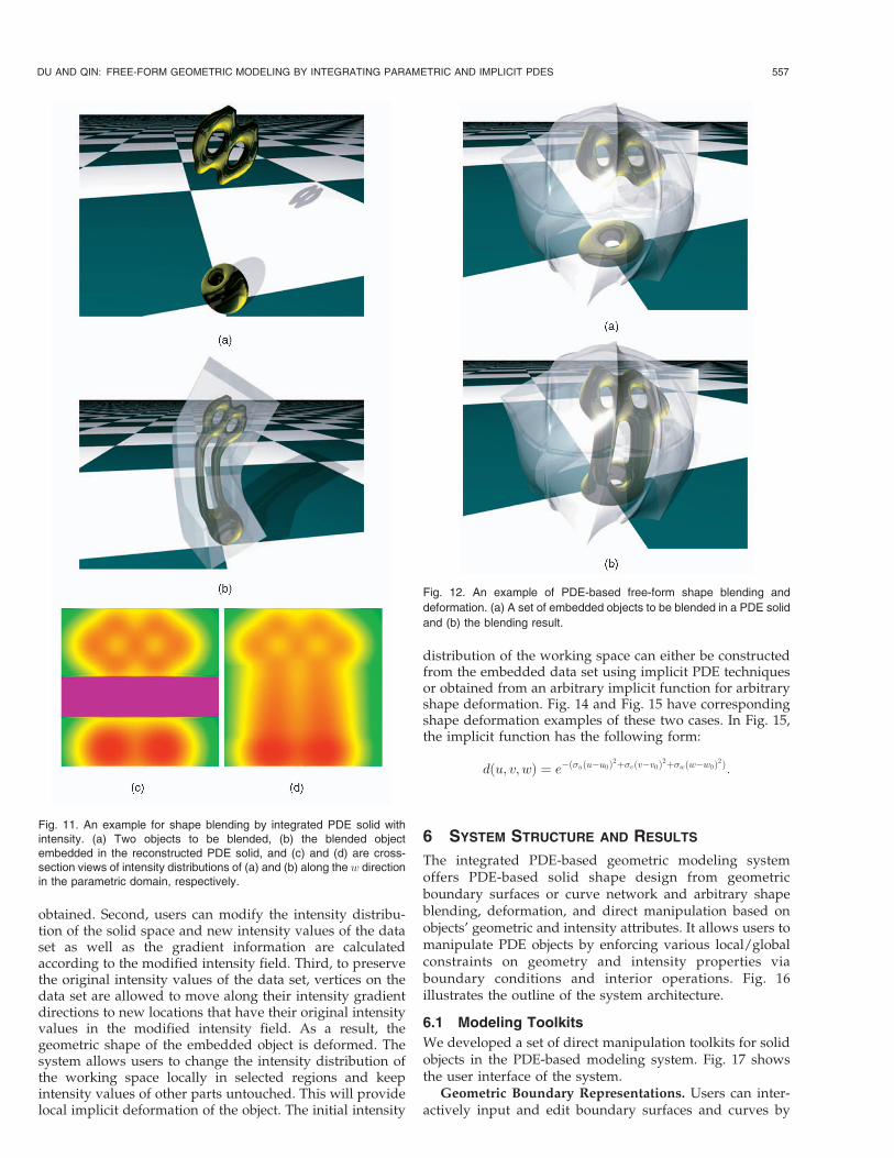
in [20], [21]. Then, the embedding geometric spaces andintensity distributions can be used as boundary constraintsfor the blended PDE solid geometry and intensity distribu-tion, respectively. Solving (11) with these boundary con-straints will result in a single geometric PDE solid blendingthe original shapes with a smoothly blended intensitydistribution for the entire solid working space. The blendedintensity field will provide a smoothly blended intensitytransition between original shapes. With any specificisovalue, an isosurface for the blended shape can bereconstructed accordingly. At the same time, the con-structed PDE solid obtained from the geometric embeddingspaces as boundary constraints offers the blended shapegeometry (Fig. 11). Moreover, because blending operationsare performed based on intensity distributions in theparametric domain, the system can provide users withdifferent blended shapes for objects embedded in deformedPDE solid working space. This allows users to obtain shapeblending and deformation at the same time. It allows morefreedom of shape manipulation for objects with arbitrarytopology. Refer to Fig. 12 and Fig. 13 for examples.

5.4 Intensity-Based Shape Deformation

The geometric shape of an embedded object in the PDEsolid can be deformed by modifying the associated intensitydistribution. When modifying the intensity distribution,intensity values of the embedded object will be changedaccordingly. Because of the correspondence between in-tensity values and geometric coordinates, to preserve theiroriginal intensity values in the modified intensity field,vertices on the object will follow the intensity modificationsto new locations in the working space, which will deformthe object’s geometric shape. We incorporate the implicitPDE modeling toolkits introduced in [21] into the system tochange the intensity values of the working space in order todeform embedded objects. The procedure is as follows:First, by initializing the intensity field of the PDE solidspace, the intensity values of an embedded data set are

556 IEEE TRANSACTIONS ON VISUALIZATION AND COMPUTER GRAPHICS, VOL. 13, NO. 3, MAY/JUNE 2007

Fig. 9. Examples of intensity initialization of PDE solids. The objects (a)

and (c) are embedded in the PDE solid working space with a color map

of intensity distribution; (b) and (d) are cross-section views of intensity

distributions in the parametric space from the w direction.

Fig. 10. An example for isosurface deformation. (a) A set of scattered

points, (b) implicit isosurface obtained from (a), and (c) and (d) are

deformed isosurfaces in different PDE solids.

obtained. Second, users can modify the intensity distribu-tion of the solid space and new intensity values of the dataset as well as the gradient information are calculatedaccording to the modified intensity field. Third, to preservethe original intensity values of the data set, vertices on thedata set are allowed to move along their intensity gradientdirections to new locations that have their original intensityvalues in the modified intensity field. As a result, thegeometric shape of the embedded object is deformed. Thesystem allows users to change the intensity distribution ofthe working space locally in selected regions and keepintensity values of other parts untouched. This will providelocal implicit deformation of the object. The initial intensity

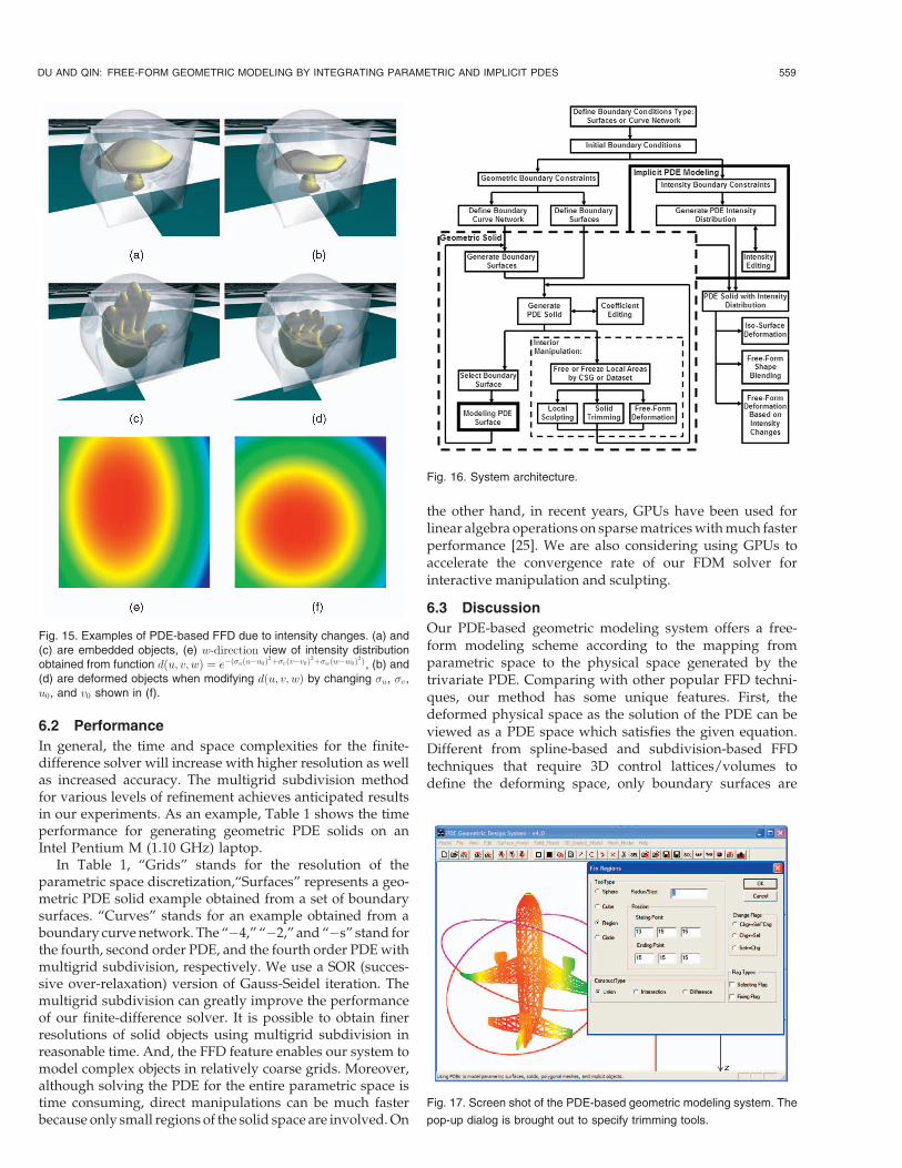
distribution of the working space can either be constructedfrom the embedded data set using implicit PDE techniquesor obtained from an arbitrary implicit function for arbitraryshape deformation. Fig. 14 and Fig. 15 have correspondingshape deformation examples of these two cases. In Fig. 15,the implicit function has the following form:

dðu; v; wÞ ¼ e�ð�uðu�u0Þ2þ�vðv�v0Þ2þ�wðw�w0Þ2Þ:

6 SYSTEM STRUCTURE AND RESULTS

The integrated PDE-based geometric modeling systemoffers PDE-based solid shape design from geometricboundary surfaces or curve network and arbitrary shapeblending, deformation, and direct manipulation based onobjects’ geometric and intensity attributes. It allows users tomanipulate PDE objects by enforcing various local/globalconstraints on geometry and intensity properties viaboundary conditions and interior operations. Fig. 16illustrates the outline of the system architecture.

6.1 Modeling Toolkits

We developed a set of direct manipulation toolkits for solidobjects in the PDE-based modeling system. Fig. 17 showsthe user interface of the system.

Geometric Boundary Representations. Users can inter-actively input and edit boundary surfaces and curves by

DU AND QIN: FREE-FORM GEOMETRIC MODELING BY INTEGRATING PARAMETRIC AND IMPLICIT PDES 557

Fig. 11. An example for shape blending by integrated PDE solid withintensity. (a) Two objects to be blended, (b) the blended objectembedded in the reconstructed PDE solid, and (c) and (d) are cross-section views of intensity distributions of (a) and (b) along the w directionin the parametric domain, respectively.

Fig. 12. An example of PDE-based free-form shape blending and

deformation. (a) A set of embedded objects to be blended in a PDE solid

and (b) the blending result.

selecting the boundary of interests and obtain PDE solidssatisfying these conditions. The system also providesvarious manipulation toolkits to deform boundary surfacesand the solid geometry will be modified accordingly.

Geometric Interior Operations. Users can also workdirectly inside the PDE solid space through: 1) interiordeformation with additional constraints inside the solid,2) trimming specified regions for complex geometry andarbitrary topology, and 3) free-form deformation based onthe mapping from the 3D parametric domain to physicalspace through trivariate PDEs.

Shape Modeling Based on Intensity Fields. We furtherintegrate scalar intensity properties with PDE solid geometryfor arbitrary shape modeling: 1) implicit PDE-based shapemodeling through free-form deformation and direct manip-ulation, 2) arbitrary shape blending by integrating geometricand intensity properties in the working space, and 3) in-tensity-based shape deformation by changing the intensitydistribution globally/locally in the PDE solid space.

Besides traditional boundary conditions of PDE techni-ques, the system allows users to specify and enforce a largevariety of additional constraints on a set of points, cross-sectional curves, and surface areas on boundary surfaces.These constraints provide more freedom to designers,making the design process of PDE solids more cost-effective. The curve-based boundary conditions make it

even easier for designers to achieve the desired shapes of

PDE solids from curve sketches. We use finite-difference

techniques because they are simple, easy to implement, and

suitable for the incorporation of complicated, flexible

constraints. Because of the finite-difference discretization,

the system allows users to enforce additional constraints

directly inside the PDE solid and apply trimming opera-

tions, which facilitate the construction of PDE objects of

arbitrary topology. The direct and free-form modeling

based on PDE solid geometry and intensity distributions

allow arbitrary shape blending and modification function-

alities for the PDE-based geometric modeling system.

558 IEEE TRANSACTIONS ON VISUALIZATION AND COMPUTER GRAPHICS, VOL. 13, NO. 3, MAY/JUNE 2007

Fig. 13. Another example of PDE-based free-form shape blending and

deformation. (a) Two objects before blending embedded in a PDE solid

and (b) the result after blending.

Fig. 14. An example for PDE-based FFD by intensity changes. (a) Anembedded shape, (b) the deformed object to preserve its originalintensity value in the locally modified intensity field, and (c) and (d) arecorresponding cross-section views of the intensity fields along thew direction for (a) and (b), respectively.

6.2 Performance

In general, the time and space complexities for the finite-difference solver will increase with higher resolution as wellas increased accuracy. The multigrid subdivision methodfor various levels of refinement achieves anticipated resultsin our experiments. As an example, Table 1 shows the timeperformance for generating geometric PDE solids on anIntel Pentium M (1.10 GHz) laptop.

In Table 1, “Grids” stands for the resolution of theparametric space discretization,“Surfaces” represents a geo-metric PDE solid example obtained from a set of boundarysurfaces. “Curves” stands for an example obtained from aboundary curve network. The “�4,” “�2,” and “�s” stand forthe fourth, second order PDE, and the fourth order PDE withmultigrid subdivision, respectively. We use a SOR (succes-sive over-relaxation) version of Gauss-Seidel iteration. Themultigrid subdivision can greatly improve the performanceof our finite-difference solver. It is possible to obtain finerresolutions of solid objects using multigrid subdivision inreasonable time. And, the FFD feature enables our system tomodel complex objects in relatively coarse grids. Moreover,although solving the PDE for the entire parametric space istime consuming, direct manipulations can be much fasterbecause only small regions of the solid space are involved. On

the other hand, in recent years, GPUs have been used forlinear algebra operations on sparse matrices with much fasterperformance [25]. We are also considering using GPUs toaccelerate the convergence rate of our FDM solver forinteractive manipulation and sculpting.

6.3 Discussion

Our PDE-based geometric modeling system offers a free-form modeling scheme according to the mapping fromparametric space to the physical space generated by thetrivariate PDE. Comparing with other popular FFD techni-ques, our method has some unique features. First, thedeformed physical space as the solution of the PDE can beviewed as a PDE space which satisfies the given equation.Different from spline-based and subdivision-based FFDtechniques that require 3D control lattices/volumes todefine the deforming space, only boundary surfaces are

DU AND QIN: FREE-FORM GEOMETRIC MODELING BY INTEGRATING PARAMETRIC AND IMPLICIT PDES 559

Fig. 15. Examples of PDE-based FFD due to intensity changes. (a) and(c) are embedded objects, (e) w-direction view of intensity distributionobtained from function dðu; v; wÞ ¼ e�ð�uðu�u0Þ2þ�vðv�v0Þ2þ�wðw�w0Þ2Þ, (b) and(d) are deformed objects when modifying dðu; v; wÞ by changing �u, �v,u0, and v0 shown in (f).

Fig. 16. System architecture.

Fig. 17. Screen shot of the PDE-based geometric modeling system. The

pop-up dialog is brought out to specify trimming tools.

necessary to form the PDE space, and the interior informa-tion will be recovered and governed by the equation itself.Second, the PDE scheme also provides a continuousdeforming space by default and modifications of any regionin the space will be smoothly propagated into its neighbor-hood. Therefore, any object embedded in the PDE space willfollow the continuous geometric distribution inside thesolid space and avoid self-intersection. Third, we alsoprovide sculpting of arbitrary interior regions for localdeformation and direct manipulation similarly to other FFDtechniques. Unlike most spline-based FFD techniques thathave to modify the control lattices based on the directmanipulations first and then deform the rest of the objectaccordingly, any sculpting operation on local regions in ourPDE model will directly affect neighboring areas accordingto the equation. However, because of the nature of FDMused in our system, interactivity is a concern whenmanipulating large regions. For improvement, we considerusing GPUs to obtain interactive operations.

In addition, the incorporation of implicit PDEs forintensity distribution inherits modeling advantages ofimplicit models into our system. Thus, we can providemodeling functionalities that are difficult for parametrictechniques such as arbitrary shape blending and shapedeformation based on intensity manipulation. Compared toalgebraic shape blending, our method offers local controland direct interference because our PDE formulation allowsadditional constraints directly enforced in local regions.

7 CONCLUSION

We present a novel geometric modeling framework thatintegrates PDE solids, surfaces, and implicit PDE models forgeneral and arbitrary shape modeling including design,deformation, sculpting, and blending. The integrated modeluses elliptic PDEs to govern both geometric and intensityproperties of solid objects. The PDE solid geometry can bedefined by either boundary surfaces or a set of curves asgeneralized boundary conditions governed by PDE surfaceformulation. The geometric PDE solid modeling techniquesallow users to manipulate objects satisfying a set of designcriteria and functional requirements with lots of degrees offreedom. The incorporation of intensity attributes to solidobjects provides modeling advantages of implicit functions tothe integrated PDE model. We developed a set of manipula-tion toolkits that support both global and local deformation ofPDE solids subject to various constraints. Our PDE-basedgeometric modeling system offers PDE-governed boundarysurface manipulations to deform the solid geometry, which

permit users to model and edit boundary PDE surfaces andthe geometric shape of corresponding PDE solid intuitivelywith ease. The deformation and trimming operations insidethe solid space provide a natural way of free-form modelingfor objects with arbitrary topology. In addition, users canmanipulate intensity distributions of the PDE solid to obtainarbitrary shape blending and deformation for embeddedobjects. Our unified PDE-based approach greatly expands thegeometric coverage and topological flexibilities of conven-tional PDE solids and implicit PDE models and improves theutility of PDE solids for modeling and design applications.With this integrated framework, it is possible to simulate realworld objects with material properties.

ACKNOWLEDGMENTS

This work was supported in part by US National ScienceFoundation (NSF) CAREER award CCR-9896123, NSF grantsIIS-0082035 and IIS-0097646, NFS grant CCR-0328930, NSFITR grant IIS-0326388, the Alfred P. Sloan Fellowship, theHonda Initiation Award, and an appointment to the NLMResearch Participation Program sponsored by the NationalLibrary of Medicine and administered by the Oak RidgeInstitute for Science and Education.

REFERENCES

[1] C.M. Hoffmann, Geometric and Solid Modeling: An Introduction.Morgan Kaufmann, 1989.

[2] M. Mortenson, Geometric Modeling, second ed. Wiley ComputerPublishing, 1997.

[3] M.I.G. Bloor and M.J. Wilson, “Generating Blend Surfaces UsingPartial Differential Equations,” Computer Aided Design, vol. 21,no. 3, pp. 165-171, 1989.

[4] M.I.G. Bloor and M.J. Wilson, “Using Partial DifferentialEquations to Generate Free-Form Surfaces,” Computer AidedDesign, vol. 22, no. 4, pp. 202-212, 1990.

[5] T.W. Lowe, M.I.G. Bloor, and M.J. Wilson, “Functionality in BlendDesign,” Computer Aided Design, vol. 22, no. 10, pp. 655-665, 1990.

[6] H. Ugail, M.I.G. Bloor, and M.J. Wilson, “Techniques forInteractive Design Using the PDE Method,” ACM Trans. Graphics,vol. 18, no. 2, pp. 195-212, 1999.

[7] J.J. Zhang and L. You, “Surface Representation Using Second,Fourth and Mixed Order Partial Differential Equations,” Proc. Int’lConf. Shape Modeling and Applications, pp. 250-256, 2001.

[8] M.I.G. Bloor and M.J. Wilson, “Functionality in Solids Obtainedfrom Partial Differential Equations,” Computing Supplement 8,pp. 21-42, 1993.

[9] H. Du and H. Qin, “Integrating Physics-Based Modeling with PDESolids for Geometric Design,” Proc. Eighth Pacific Conf. ComputerGraphics and Applications (Pacific Graphics ’01), pp. 198-207, 2001.

[10] J. Bloomenthal, C. Bajaj, J. Blinn, M.-P. Cani-Gascuel, A. Rock-wood, B. Wyvill, and G. Wyvill, Introduction to Implicit Surfaces.Morgan Kaufmann, 1997.

[11] H. Du and H. Qin, “Direct Manipulation and Interactive Sculptingof PDE Surfaces,” Computer Graphics Forum, vol. 19, no. 3,pp. C261-C270, 2000.

[12] H. Du and H. Qin, “Dynamic PDE Surfaces with Flexible andGeneral Constraints,” Proc. Eighth Pacific Conf. Computer Graphicsand Applications (Pacific Graphics ’00), pp. 213-222, 2000.

[13] H. Du and H. Qin, “Dynamic PDE-Based Surface Design UsingGeometric and Physical Constraints,” Graphical Models, vol. 67,no. 1, pp. 43-71, 2005.

[14] T. Sederberg and S. Parry, “Free-Form Deformation of SolidGeometric Models,” Proc. SIGGRAPH ’86, pp. 151-158, 1986.

[15] S. Coquillart, “Extended Free-Form Deformation: A SculptingTool for 3D Geometric Modeling,” Proc. SIGGRAPH ’90, pp. 187-196, 1990.

[16] W.H. Hsu, J.F. Hughes, and H. Kaufman, “Direct Manipulation ofFree-Form Deformation,” Proc. SIGGRAPH ’92, pp. 177-184, 1992.

560 IEEE TRANSACTIONS ON VISUALIZATION AND COMPUTER GRAPHICS, VOL. 13, NO. 3, MAY/JUNE 2007

TABLE 1CPU Time (in Seconds) for Generating PDE Solid Geometry

with Different Types of Boundary Conditions

[17] R. MacCracken and K.I. Joy, “Free-Form Deformations withLattices of Arbitrary Topology,” Proc. SIGGRAPH ’96, pp. 181-188, 1996.

[18] K. Singh and E. Fiume, “Wires: A Geometric DeformationTechnique,” Proc. SIGGRAPH ’98, pp. 405-414, 1998.

[19] J. Hua and H. Qin, “Scalar-Field-Guided Adaptive ShapeDeformation and Animation,” The Visual Computer, 2003.

[20] H. Du and H. Qin, “Interactive Shape Design Using VolumetricImplicit PDEs,” Proc. Eighth ACM Symp. Solid Modeling andApplications, pp. 235-246, 2003.

[21] H. Du and H. Qin, “A Shape Design System Using VolumetricImplicit PDEs,” Computer-Aided Design, vol. 36, no. 11, pp. 1101-1116, 2004.

[22] G. Strang, Introduction to Applied Mathematics. Wellesley-Cam-bridge Press, 1986.

[23] N. Dyn, D. Levin, and J.A. Gregory, “A Butterfly SubdivisionScheme for Surface Interpolation with Tension Control,” ACMTrans. Graphics, vol. 9, no. 2, pp. 160-169, 1990.

[24] W.E. Lorensen and H.E. Cline, “Marching Cubes: A HighResolution 3D Surface Construction Algorithm,” Proc. SIGGRAPH’87, pp. 163-169, 1987.

[25] J. Kruger and R. Westermann, “Linear Algebra Operators for GPUImplementation of Numerical Algorithms,” ACM Trans. Graphics,vol. 22, no. 3, pp. 908-916, 2003.

Haixia Du received the BS degree in computerscience from Jilin University in Changchun,China, in 1995, the ME degree in computerscience from the Institute of Mathematics,Chinese Academy of Sciences in Beijing, China,in 1998, and the MS and PhD degrees incomputer science from the State University ofNew York at Stony Brook (Stony Brook Uni-versity) in 2000 and 2004. She is a postdoctoralfellow in the 3D Informatics Group of the Office

of High Performance Computing and Communications at the NationalLibrary of Medicine, National Institutes of Health. Her research interestsinclude geometric and physics-based modeling, scientific and informa-tion visualization, and medical imaging, with emphasis on applying PDE-based techniques for geometric modeling, including shape design,reconstruction, metamorphosis, and simplification, and medical imageprocessing including image filtering, segmentation, and registration.Detailed information about Dr. Haixia Du can be found at her Web site:http://www.haixiadu.net.

Hong Qin received the BS degree and the MSdegree in computer science from Peking Uni-versity in Beijing, China. He received the PhD(1995) degree in computer science from theUniversity of Toronto. He is a full professor (withtenure) of computer science in the Departmentof Computer Science at the State University ofNew York at Stony Brook (Stony Brook Uni-versity). During his years at the University ofToronto (UofT), he received the UofT Open

Doctoral Fellowship. In 1997, Professor Qin was awarded the USNational Science Foundation (NSF) CAREER Award. In December2000, Professor Qin received the Honda Initiation Grant Award. InFebruary 2001, Professor Qin was selected as an Alfred P. SloanResearch Fellow by the Sloan Foundation. In 2005, Professor Qinserved as the general cochair for Computer Graphics International 2005(CGI 2005) held on 22-24 June 2005 at SUNY Stony Brook. Currently,he is an associate editor for IEEE Transactions on Visualization andComputer Graphics (TVCG) and he is also on the editorial board of TheVisual Computer (International Journal of Computer Graphics). He is theconference cochair for the ACM Solid and Physical Modeling Sympo-sium 2007 (to be held at Tsinghua University, Beijing, China). Hisresearch interests include geometric and solid modeling, graphics,physics-based modeling and simulation, computer aided geometricdesign, human-computer interaction, visualization, and scientific com-puting. Detailed information about Dr. Hong Qin can be found from hisWeb site: http://www.cs.sunysb.edu/qin. He is a member of the IEEE.

. For more information on this or any other computing topic,please visit our Digital Library at www.computer.org/publications/dlib.

DU AND QIN: FREE-FORM GEOMETRIC MODELING BY INTEGRATING PARAMETRIC AND IMPLICIT PDES 561