IEICE Communications Express, Vol.5, No.4, 95 Synchronization … · 2016. 3. 28. · Abstract: The...

Synchronization algorithm ofasynchronously captureddata packets andinstantaneous power-linefrequency data for PLCanalysis

Daijiro Ueno1, Kenji Kita2, Yuji Sano1,3, Tadahiko Kimoto1,3,Hiroyasu Ishikawa4, and Hideyuki Shinonaga1,3a)1 Graduate School of Science and Engineering, Toyo University,

2100 Kujirai, Kawagoe, Saitama 350–8585, Japan2 Malaysia Japan Higher Education Program, University of Kuala Lumpur,

Lot 2333, Jalan Semenyih, Bandar Tasik Kesuma, Beranang, Selangor,

43700, Malaysia3 Faculty of Science and Engineering, Toyo University,

2100 Kujirai, Kawagoe, Saitama 350–8585, Japan4 College of Engineering, Nihon University,

1 Nakagawa, Tamuramachi, Koriyama, Fukushima 963–8642, Japan

a) [email protected]

Abstract: The instantaneous power-line frequency synchronized superim-

posed chart was proposed by the authors to visualize the effects of an AC

adapter for PLC (Power Line Communications) transmission. In order to

most properly draw the superimposed chart, it is requisite to synchronize

data packets and instantaneous power-line frequency data, which are asyn-

chronously captured by separate PCs (Personal Computers). This paper

proposes a synchronization algorithm for these data, and shows the effective-

ness of the proposed algorithm. Furthermore, an algorithm to compensate the

fixed frequency measurement error made by a digital multi-meter is pro-

posed. Finally, it is shown that the communications forbidden time, the

duration when PLC burst signals are not correctly received due to the effects

of the AC adapter, is properly shown by adopting the proposed two

algorithms as well as how burst signals containing different number of

data packets are transmitted in the moments other than the communications

forbidden time.

Keywords: power line communications, data synchronization algorithm

Classification: Transmission Systems and Transmission Equipment for

Communications© IEICE 2016DOI: 10.1587/comex.2016XBL0008Received January 12, 2016Accepted January 26, 2016Publicized February 10, 2016Copyedited April 1, 2016

95

IEICE Communications Express, Vol.5, No.4, 95–101

References

[1] F. J. C. Corripio, J. A. C. Arrabal, L. D. del Río, and J. T. E. Muñoz, “Analysisof the cyclic short-term variation of indoor power line channels,” IEEE J. Sel.Areas Commun., vol. 24, no. 7, pp. 1327–1338, July 2006. DOI:10.1109/JSAC.2006.874402

[2] D. Umehara, T. Hayasaki, S. Denno, and M. Morikura, “Influences ofperiodically switching channels synchronized with power frequency on PLCequipment,” J. Commun., vol. 4, no. 2, pp. 108–118, March 2009. DOI:10.4304/jcm.4.2.108-118

[3] G. Masuda, H. Yanagisawa, and H. Shinonaga, “Packet capture analysis ofpacket errors induced by AC adapter in power line communications system,”IEICE Gen. Conf. ’11, B-4-45. (In Japanese)

[4] S. Mori, G. Masuda, and H. Shinonaga, “Packet capture analysis of effects ofAC adapter in power line communications (IV),” IEICE Gen. Conf. ’13, B-8-6.(In Japanese)

[5] NLANR/DAST, ESnet, “What is iperf/iperf3,” https://iperf.fr/, accessed Sep.22, 2015.

[6] Panasonic, “HD-PLC (BL-PA310 series),” http://panasonic.jp/p3/plc/pa310.html, accessed Sep. 22, 2015.

[7] Wireshark Foundation, “Download Wireshark,” https://www.wireshark.org/download.html, accessed Sep. 22, 2015.

[8] SANWA Electronic Measurement Instrument Company, “PC 7000,” http://www.sanwa-meter.co.jp/japan/items/detail.php?id=13, accessed Sep.22, 2015.

[9] Y. Baba, Basics of Statistics and Probability, Makino Bookstore, Tokyo, 2002.(In Japanese)

1 Introduction

A PLC system employs power-lines as transmission lines, and transmits burst

signals containing multiple data packets with high throughput. Some AC adapters

of mobile phones affect transmission of the PLC signals. It was reported that two

kinds of transfer functions periodically appear, synchronized with a half-cycle of

the power-line frequency [1, 2]. It was found by the authors that the communica-

tions forbidden time, the duration when PLC burst signals are not correctly

received, appears once in a half-cycle of the power-line frequency due to the

effects of the AC adapter [3]. A chart named the instantaneous power-line

frequency synchronized superimposed chart, referred to as the superimposed chart,

was also proposed by the authors [4] to visualize the communications forbidden

time as well as how burst signals containing different number of data packets are

transmitted in the moments other than the forbidden time. Note that the objective of

the superimposed chart is to illustrate the actual computer communications through

the PLC transmission affected by the AC adapter. To draw the superimposed chart

properly, it is requisite to synchronize asynchronously captured data packets and

instantaneous power-line frequency data. This paper proposes a synchronization

algorithm for these data, and shows the effectiveness of the proposed algorithm.© IEICE 2016DOI: 10.1587/comex.2016XBL0008Received January 12, 2016Accepted January 26, 2016Publicized February 10, 2016Copyedited April 1, 2016

96


http://dx.doi.org/10.1109/JSAC.2006.874402




http://dx.doi.org/10.4304/jcm.4.2.108-118






https://iperf.fr/

https://iperf.fr/

http://panasonic.jp/p3/plc/pa310.html



https://www.wireshark.org/download.html





http://www.sanwa-meter.co.jp/japan/items/detail.php?id=13







2 Synchronization algorithm for asynchronously captured data

packets and instantaneous power-line frequency data

2.1 Measurement network configuration

Fig. 1(a) depicts the measurement network configuration. UDP (User Datagram

Protocol) data packets with a rate of 30Mbit/s are generated by data packet

generating software [5], supplied to the Tx (Transmit) HD (High-Definition)-

PLC adapter [6], transmitted in a form of a burst signal, nominally containing 5

or 6 data packets, and received by the Rx (Receive) PLC adapter. The data packets

Fig. 1. Measurement network configuration and the superimposedcharts under the condition that the captured data are notsynchronized.

© IEICE 2016DOI: 10.1587/comex.2016XBL0008Received January 12, 2016Accepted January 26, 2016Publicized February 10, 2016Copyedited April 1, 2016

97


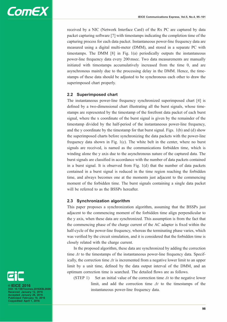
received by a NIC (Network Interface Card) of the Rx PC are captured by data

packet capturing software [7] with timestamps indicating the completion time of the

capturing process for each data packet. Instantaneous power-line frequency data are

measured using a digital multi-meter (DMM), and stored in a separate PC with

timestamps. The DMM [8] in Fig. 1(a) periodically outputs the instantaneous

power-line frequency data every 200msec. Two data measurements are manually

initiated with timestamps accumulatively increased from the time 0, and are

asynchronous mainly due to the processing delay in the DMM. Hence, the time-

stamps of these data should be adjusted to be synchronous each other to draw the

superimposed chart properly.

2.2 Superimposed chart

The instantaneous power-line frequency synchronized superimposed chart [4] is

defined by a two-dimensional chart illustrating all the burst signals, whose time-

stamps are represented by the timestamp of the forefront data packet of each burst

signal, where the x coordinate of the burst signal is given by the remainder of the

timestamp divided by the half-period of the instantaneous power-line frequency,

and the y coordinate by the timestamp for that burst signal. Figs. 1(b) and (d) show

the superimposed charts before synchronizing the data packets with the power-line

frequency data shown in Fig. 1(c). The white belt in the center, where no burst

signals are received, is named as the communications forbidden time, which is

winding alone the y axis due to the asynchronous nature of the captured data. The

burst signals are classified in accordance with the number of data packets contained

in a burst signal. It is observed from Fig. 1(d) that the number of data packets

contained in a burst signal is reduced in the time region reaching the forbidden

time, and always becomes one at the moments just adjacent to the commencing

moment of the forbidden time. The burst signals containing a single data packet

will be referred to as the BSSPs hereafter.

2.3 Synchronization algorithm

This paper proposes a synchronization algorithm, assuming that the BSSPs just

adjacent to the commencing moment of the forbidden time align perpendicular to

the y axis, when these data are synchronized. This assumption is from the fact that

the commencing phase of the charge current of the AC adapter is fixed within the

half-cycle of the power-line frequency, whereas the terminating phase varies, which

was verified by the circuit simulation, and it is considered that the forbidden time is

closely related with the charge current.

In the proposed algorithm, these data are synchronized by adding the correction

time �t to the timestamps of the instantaneous power-line frequency data. Specif-

ically, the correction time �t is incremented from a negative lower limit to an upper

limit by a unit time, defined by the data output interval of the DMM, and an

optimum correction time is searched. The detailed flows are as follows.

(STEP 1) Set an initial value of the correction time �t to the negative lower

limit, and add the correction time �t to the timestamps of the

instantaneous power-line frequency data.© IEICE 2016DOI: 10.1587/comex.2016XBL0008Received January 12, 2016Accepted January 26, 2016Publicized February 10, 2016Copyedited April 1, 2016

98


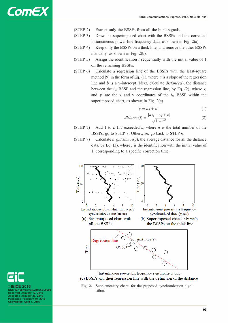
(STEP 2) Extract only the BSSPs from all the burst signals.

(STEP 3) Draw the superimposed chart with the BSSPs and the corrected

instantaneous power-line frequency data, as shown in Fig. 2(a).

(STEP 4) Keep only the BSSPs on a thick line, and remove the other BSSPs

manually, as shown in Fig. 2(b).

(STEP 5) Assign the identification i sequentially with the initial value of 1

on the remaining BSSPs.

(STEP 6) Calculate a regression line of the BSSPs with the least-square

method [9] in the form of Eq. (1), where a is a slope of the regression

line and b is a y-intercept. Next, calculate distance(i), the distance

between the ith BSSP and the regression line, by Eq. (2), where xi

and yi are the x and y coordinates of the ith BSSP within the

superimposed chart, as shown in Fig. 2(c).

y ¼ ax þ b ð1Þ

distanceðiÞ ¼ jaxi � yi þ bjffiffiffiffiffiffiffiffiffiffiffiffiffi1 þ a2

p ð2Þ

(STEP 7) Add 1 to i. If i exceeded n, where n is the total number of the

BSSPs, go to STEP 8. Otherwise, go back to STEP 6.

(STEP 8) Calculate avg.distance(j), the average distance for all the distance

data, by Eq. (3), where j is the identification with the initial value of

1, corresponding to a specific correction time.

Fig. 2. Supplementary charts for the proposed synchronization algo-rithm.


99


avg:distanceðjÞ ¼

Xn

i¼1distanceðiÞ

nð3Þ

(STEP 9) Add 1 to j. Add the unit time, the interval time of the instantaneous

power-line frequency data output by the DMM, to the correction time

�t, add the renewed correction time �t to the timestamps of the

instantaneous power-line frequency data, and return to STEP 3. If

the correction time �t exceeded the upper limit, go to STEP 10.

(STEP 10) Determine the correction time �t which minimizes

avg.distance(j) as the optimum correction time, and finish the

algorithm.

3 Results and discussions

The data packets and instantaneous power-line frequency data were applied for

the synchronization algorithm. The unit time in STEP 9 was set to 200msec, and

the lower and upper limits were set to −3.0 and 0.0 sec, respectively. Fig. 3(a)

shows the calculated average distance as a function of the correction time �t. The

burst signals just adjacent to the commencing moment of the forbidden time align

most linearly when the average distance takes the minimum and optimum value

of −2.2 sec. This time difference is mainly due to the processing delay of the

DMM, including the error made by the manually and asynchronously initiated

measurements.

The DMM generates a measurement error as specified in the specifications [8].

The error was assumed to be fixed during the measurements, and searched among

the error range specified in the specifications by compensating specific fixed errors

and by observing the resultant superimposed charts. In the example calculation

using the data with the optimum �t of −2.2 sec, the error was determined to be

�8:3 � 10�4Hz. The superimposed chart after compensating the measurement error

is shown in Fig. 3(b). The forbidden time is shown as a white belt perpendicular to

the horizontal axis, and how burst signals containing different number of data

packets are transmitted in the moments other than the forbidden time is clearly

illustrated. The white forbidden time belt is strongly correlated with the purple belt,

where the number of data packets is typically 11 or 12, and the commencing

moments of these two belts are separated by 2.26msec, which is the typical burst

signal interval. By comparing Fig. 1(b) and Fig. 3(b), the effectiveness of the

proposed two algorithms is clarified as explained above.

It is also verified that the BSSPs always appear at the moments just before the

commencing moment of the forbidden time, as long as the electric appliances

generate the forbidden time, those include some of LED lamps, electric fans, and

portable game players and so on.


100


4 Conclusions

The synchronization algorithm for the asynchronously captured data packets and

instantaneous power-line frequency data is proposed. The example calculation

showed the effectiveness of the proposed algorithm. Furthermore, the fixed

frequency measurement error of the DMM was searched, determined and compen-

sated, and the resultant superimposed chart properly showed the communications

forbidden time belt as well as how burst signals containing different number of data

packets are transmitted in the moments other than the forbidden time.

Fig. 3. Example calculation results using the proposed algorithms.


101


Experimental validation ofcommunication disturbanceobserver for networkedcontrol systems withinformation losses

Ryusuke Imaia) and Ryogo KuboDepartment of Electronics and Electrical Engineering, Keio University,

3–14–1 Hiyoshi, Kohoku-ku, Yokohama-shi, Kanagawa 223–8522, Japan


Abstract: Networked control systems (NCSs) using the Internet will soon

become widespread. In NCSs, time delays and information losses cause

system performance degradation and destabilization. It is known that a

communication disturbance observer (CDOB)-based compensator can esti-

mate and suppress the effect of time delays on the system as a network

disturbance. We applied a CDOB-based compensator to NCSs with not only

time delays but also information losses and theoretically analyzed the

information-loss compensation scheme. However, the performance of the

CDOB-based compensator for only information losses in real NCSs has not

been experimentally evaluated. This letter demonstrates an information-loss

compensation scheme using a CDOB for NCSs. Experiments using a

networked motion control system show that the CDOB-based compensator

can estimate and suppress the effect of information losses on an NCS.

Keywords: sensor-actuator network, machine-to-machine, motion control,

networked control system, information loss

Classification: Network

References

[1] J. Baillieul and P. J. Antsaklis, “Control and communication challenges innetworked real-time systems,” Proc. IEEE, vol. 95, no. 1, pp. 9–28, Jan. 2007.DOI:10.1109/JPROC.2006.887290

[2] R. A. Gupta and M.-Y. Chow, “Networked control system: overview andresearch trends,” IEEE Trans. Ind. Electron., vol. 57, no. 7, pp. 2527–2535, Jul.2010. DOI:10.1109/TIE.2009.2035462

[3] O. J. M. Smith, “A controller to overcome dead time,” ISA J., vol. 6, no. 2,pp. 28–33, Oct. 1959.

[4] C.-L. Lai and P.-L. Hsu, “Design the remote control system with the time-delayestimator and the adaptive Smith predictor,” IEEE Trans. Ind. Informat., vol. 6,no. 1, pp. 73–80, Feb. 2010. DOI:10.1109/TII.2009.2037917

[5] K. Natori and K. Ohnishi, “A design method of communication disturbanceobserver for time-delay compensation,taking the dynamic property of networkdisturbance into account,” IEEE Trans. Ind. Electron., vol. 55, no. 5,


102


http://dx.doi.org/10.1109/JPROC.2006.887290




http://dx.doi.org/10.1109/TIE.2009.2035462




http://dx.doi.org/10.1109/TII.2009.2037917




pp. 2152–2168, May 2008. DOI:10.1109/TIE.2008.918635[6] K. Natori, R. Oboe, and K. Ohnishi, “Stability analysis and practical design

procedure of time delayed control systems with communication disturbanceobserver,” IEEE Trans. Ind. Informat., vol. 4, no. 3, pp. 185–197, Aug. 2008.DOI:10.1109/TII.2008.2002705

[7] R. Imai and R. Kubo, “Introducing jitter buffers in networked control systemswith communication disturbance observer under time-varying communicationdelays,” Proc. 41st Annual Conference of the IEEE Industrial ElectronicsSociety (IECON 2015), pp. 2956–2961, Nov. 2015.

[8] R. Kubo and K. Natori, “Dependable networked motion control usingcommunication disturbance observer,” Proc. 27th International TechnicalConference on Circuits/Systems, Computers and Communications (ITC-CSCC2012), pp. 1–4, Jul. 2012.

[9] A. Codrean, O. Stefan, and T.-L. Dragomir, “Design, analysis and validation ofan observer-based delay compensation structure for a network control system,”Proc. 20th Mediterranean Conference on Control & Automation (MED 2012),pp. 928–934, Jul. 2012. DOI:10.1109/MED.2012.6265757

1 Introduction

In recent years, the rapid spread of high-performance computing technologies and

broadband communication networks has accelerated the realization of various

networked control systems (NCSs) [1, 2]. NCSs are categorized into “control of

network” and “control over network.” As one of the “control over network”

technologies, networked motion control is currently an attractive research topic.

For example, teleoperation robots, which are utilized in space, under water, or in

nuclear power plants, have been developed based on networked motion control

technologies.

In NCSs, the existence of time delays and information losses in the feedback

control loop is a significant problem in the design of an appropriate controller. The

Smith predictor (SP) is a classical time-delay compensator using a time-delay

model [3]. The SP needs a precise time-delay model, and the difference between the

model and actual time delay causes system performance degradation and destabi-

lization. The adaptive Smith predictor (ASP) measures time delays and updates the

time-delay model to remove the modeling error of time delays [4]. Natori et al. [5,

6] proposed a communication disturbance observer (CDOB)-based compensator to

estimate and suppress the effect of time delays on NCSs without any time-delay

models. In addition, the combination of a CDOB and jitter buffers improved the

performance of time-delay compensation scheme [7].

Since the number of NCSs using imperfect networks, such as the Internet and

wireless networks, are expected to increase in the future, an effective compensator

of information losses to build more dependable networked motion control systems

is required. However, the behavior of conventional time-delay compensators, i.e.,

the SP, ASP, and CDOB, when information losses occur has not been analyzed. The

authors previously applied the conventional time-delay compensators to NCSs with

not only time delays but also information losses [8]. In [8], it was theoretically

shown that only a CDOB can compensate the effect of the information losses on


103










http://dx.doi.org/10.1109/MED.2012.6265757




NCSs. Codrean et al. [9] utilized the CDOB in the experiments, where there are

time delays and information losses. However, the effects of time delays and

information losses in NCSs with the CDOB have not been evaluated separately.

It is very important to separately discuss the effects of information losses and time

delays when we design an appropriate network for NCSs.

This letter briefly describes the concept of the ND including information losses

proposed in [8] and experimentally evaluates the CDOB-based compensator in an

NCS when only information losses exist. Experiments using a networked position

control system, which comprises a rotary motor and virtual lossy networks, show

that the CDOB-based compensator can estimate and suppress the effect of the

information losses on the NCS.

2 Networked motion control

This section describes a networked position control system comprising a motor and

a robust control technique using a disturbance observer (DOB).

2.1 Position control system

The networked position control system of a motor comprises the controller GC,

remote system GP, and network elements, as shown in Fig. 1. In this figure, xcmd,

xres, and fref are the position command, position response, and force reference,

respectively. The subscript d denotes the value after passing through the network

element. The remote system includes a DOB to realize robust motion control. The

network elements include time delays, T1 and T2, and information losses L1 and L2.

The value of each of the parameters L1 and L2 is stochastically 0 or 1.

As one of the position controllers, a proportional-derivative (PD) controller can

be implemented as

GC ¼ JnðKp þ KdsÞ; ð1Þwhere Jn, Kp, Kd, and s denote a moment-of-inertia model of the motor, a

proportional gain, a derivative gain, and the Laplace operator, respectively.

The transfer function of the total control system shown in Fig. 1 is expressed as

xres

xcmd¼ GCGPL1e

�T1s

1 þ GCGPLe�Ts; ð2Þ

Fig. 1. Networked position control system with DOB.


104


where T ¼ T1 þ T2 and L ¼ L1L2. The denominator of the transfer function

includes time-delay and information-loss elements. The network elements must

be considered in the design of the controller GC.

2.2 DOB

Motion control systems include various uncertainties and disturbances, e.g., the

parameter variation of moment of inertia, �J, the parameter variation of torque

constant, �Kt, and external force, fext. In this study, a DOB was implemented to

suppress uncertainties and disturbances. The DOB can estimate and compensate the

uncertainties and disturbances as a disturbance force fdis. The disturbance force

estimated by the DOB, fdis, is expressed as

fdis ¼ gdobs þ gdob

fdis; ð3Þ

where gdob is the cut-off frequency of the low-pass filter (LPF). The DOB supresses

the disturbance fdis ideally if the cut-off frequency gdob is sufficiently large. In this

study, we assumed the remote system GP with the DOB is given as GP ¼ 1Jns2

.

3 Information-loss compensation using CDOB

This section describes the concept of a network disturbance (ND) and a CDOB-

based compensator for NCSs with time delays and information losses. A block

diagram of the networked position control system with the CDOB is shown in

Fig. 2.

The CDOB-based compensator can estimate and suppress the effect of time

delays and information losses on the system as the ND fnd. The ND is expressed as

fnd ¼ ð1 � Le�TsÞfref : ð4ÞWhen the remote system model GP is equal to the actual remote system GP, the

output of the CDOB, xcmp, is calculated as

xcmp ¼ gcdobs þ gcdob

GPfnd ; ð5Þ

where gcdob denotes the cut-off frequency of the LPF. The effect of the ND is

estimated by the compensation signal xcmp, if the cut-off frequency gcdob is

Fig. 2. Networked position control system with CDOB.


105


sufficiently large. In this study, a first-order LPF was used as the first demonstra-

tion. The LPF is generally designed on the basis of the ND characteristics.

The transfer function of the total control system shown in Fig. 2 is expressed as

xres

xcmd¼ GCGPL1e

�T1s

1 þ GCGP: ð6Þ

The denominator of the transfer function does not include any time-delay and

information-loss elements. The controller GC can be designed without considering

the network elements.

4 Experiments

In this section, the experimental system and experimental results are presented to

verify the CDOB-based compensation scheme under information losses.

4.1 Setup

In the experiments, as shown in Fig. 3(a), the angular position of the rotary motor

was controlled by the PD controller with the DOB over the virtual network with

information losses. For example, in wireless NCSs, the controller is usually

implemented on the base station side. The assumption of information losses on

the feedback path is reasonable, since packet losses occur mainly in the upstream

direction.

The moment-of-inertia model Jn, proportional gain Kp, derivative gain Kd, cut-

off frequency of the DOB gdob, and cut-off frequency of the CDOB gcdob were set to

0.0166 kg·m2, 400, 40, 100 rad/s, and 100 rad/s, respectively. The feedback gains

were determined such that they provided a critical damping response. The sampling

period of the control system was set to 1ms. The time delays were not considered

to verify the performance of information-loss compensation, i.e., T1 ¼ T2 ¼ 0ms.

Uniformly distributed information losses were emulated on the feedback path with

a loss rate of 90% or 99%, i.e., L2 was set to 0 at a frequency of the loss rate, and L1was always set to 1.

4.2 Results

The results of experiments without the CDOB are shown in Figs. 3(b) and 3(c), and

the results with the CDOB are shown in Figs. 3(d) and 3(e). Figs. 3(b) and 3(d)

show the results when the loss rate was set to 90% and Figs. 3(c) and 3(e) show the

results when it was set to 99%. The results without the CDOB did not converge to

the command when the loss rate was 99%, whereas they did when the loss rate was

90%. The results with the CDOB converged to the command with some steady-

state errors independently of the loss rate. The steady-state errors are caused by the

effect of the modeling error between the remote system model GP and the actual

remote system GP, and the filter design of the CDOB. It was confirmed that the

CDOB could compensate the effect of information losses in real motion control

systems while generating steady-state errors.


106


5 Conclusion

This letter demonstrated an information-loss compensation scheme using a CDOB

for networked motion control systems. The experiments using the networked

position control system of a rotary motor showed that the CDOB-based compen-

sator could compensate the effect of the information losses while generating steady-

state errors.

Our further study includes the application of the CDOB-based compensation

scheme to NCSs over the Internet and the consideration of the time-delay and

information-loss characteristics of various network systems in the design of the

LPFs of the DOB and CDOB to reduce the steady-state errors.

Acknowledgment

This research was supported in part by Kenjiro Takayanagi Foundation.

Fig. 3. Experimental results.


107


Bi-generalized space shiftkeying over MIMO channels

Binh Vo and Ha H. Nguyena)

Department of ECE, University of Saskatchewan, Saskatoon, Canada S7N 5A9


Abstract: Bi-space shift keying (BiSSK) can increase the spectral effi-

ciency of space shift keying (SSK) but requiring a large number of available

transmit antennas. A new SSK-based modulation scheme is proposed which

requires a smaller number of transmit antennas than what required in BiSSK

to deliver the same transmission rate at a negligible performance loss. The

proposed scheme is obtained by multiplexing two in-phase and quadrature

generalized SSK (GSSK) streams and optimizing the carrier signals trans-

mitted by the activated antennas. Performance of the proposed scheme is

compared with other SSK-based schemes via minimum Euclidean distance

analysis and computer simulation.

Keywords: MIMO channels, spatial modulation, space shift keying

Classification: Wireless Communication Technologies

References

[1] R. Mesleh, H. Haas, C. W. Ahn, and S. Yun, “Spatial modulation— a new lowcomplexity spectral efficiency enhancing technique,” ChinaCom, Oct. 2006.DOI:10.1109/CHINACOM.2006.344658

[2] J. Jeganathan, A. Ghrayeb, L. Szczecinski, and A. Ceron, “Space shift keyingmodulation for mimo channels,” IEEE Trans. Wireless Commun., vol. 8,pp. 3692–3703, July 2009. DOI:10.1109/TWC.2009.080910

[3] J. Jeganathan, A. Ghrayeb, and L. Szczecinski, “Generalized space shift keyingmodulation for MIMO channels,” IEEE PIMRC, pp. 1–5, Sept. 2008. DOI:10.1109/PIMRC.2008.4699782

[4] H.-W. Liang, R. Chang, W.-H. Chung, H. Zhang, and S.-Y. Kuo, “Bi-space shiftkeying modulation for MIMO systems,” IEEE Commun. Lett., Aug. 2012.DOI:10.1109/LCOMM.2012.061912.120448

[5] S. Fang, L. Li, S. Hu, and G. Feng, “Layered space shift keying modulation overMIMO channels,” Proc. IEEE Int. Conf. Commun., June 2015. DOI:10.1109/ICC.2015.7248643

[6] J. G. Proakis, Digital Communications, McGraw-Hill, 1998.[7] M.-S. Alouini and A. Goldsmith, “A unified approach for calculating error rates

of linearly modulated signals over generalized fading channels,” IEEE Trans.Commun., vol. 47, pp. 1324–1334, Sept. 1999. DOI:10.1109/26.789668

[8] G. B. Giannakis and Z. Liu, Space-Time Coding for Broadband WirelessCommunications, Wiley-Interscience, 2007.

[9] R. Chang, S.-J. Lin, and W.-H. Chung, “New space shift keying modulation withhamming code-aided constellation design,” IEEE Wireless Commun. Lett.,vol. 1, pp. 2–5, Feb. 2012. DOI:10.1109/WCL.2012.102711.110037


108


http://dx.doi.org/10.1109/CHINACOM.2006.344658




http://dx.doi.org/10.1109/TWC.2009.080910




http://dx.doi.org/10.1109/PIMRC.2008.4699782




http://dx.doi.org/10.1109/LCOMM.2012.061912.120448





http://dx.doi.org/10.1109/ICC.2015.7248643





http://dx.doi.org/10.1109/26.789668

http://dx.doi.org/10.1109/26.789668

http://dx.doi.org/10.1109/26.789668

http://dx.doi.org/10.1109/WCL.2012.102711.110037





1 Introduction

In a MIMO system, when data is simultaneously transmitted on the same frequency

band from multiple transmit antennas, inter-channel interference (ICI) exits. To

completely eliminate ICI, [1] proposed a technique, called spatial modulation (SM),

in which only one antenna is activated at any transmission time. With this strategy,

the antenna index also involves in the process of sending data to the receiver. To

further reduce the decoding complexity, amplitude/phase modulation symbols are

removed and data is solely conveyed by antenna indices. This method is referred to

as SSK [2]. Although having very low decoding complexity, the drawback of SSK

is low spectral efficiency. There are many recent studies on increasing the spectral

efficiency of SSK. For example, the generalized SSK (GSSK) [3] activates more

than one antenna to yield a larger number of codewords. The spectral efficiency of

GSSK is blog2ðNt

ntÞc bits/sec/Hz, where Nt is the number of available transmit

antennas while nt is the number of activated antennas. BiSSK [4] is another scheme

that doubles the rate of SSK by multiplexing two orthogonal channels: in-phase and

quadrature channels. The transmission on each channel is determined by the SSK

rule. Recently, another scheme that also uses the multiplexing technique to enhance

the spectral efficiency is layered-SSK (LSSK) [5]. In LSSK, the layers are

determined by the SSK rule and multiplexing is performed by adding/dropping

active antennas.

The new scheme proposed in this paper, termed bi-generalized SSK (BiGSSK),

employs GSKK rule for each in-phase/quadrature data stream. As such, BiGSSK

has the same advantage of low detection complexity as with SSK, while doubling

the transmission rate of GSSK. By optimizing the signals transmitted over activated

antennas, it is shown that such spectral efficiency advantage of BiGSSK is

compromised only by a negligible performance loss. Numerical results and

performance comparison with GSSK, BiSSK, LSSK demonstrate the efficiency

of the proposed BiGSSK.

2 System model and performance analysis

The baseband input/output signal model for a Nt � Nr MIMO system operating over

a frequency-flat block fading channel and employing SSK-based modulation is

y ¼ffiffiffiffiffiEs

pHx þ n: ð1Þ

Here x is a Nt � 1 transmit symbol vector comprising of nonzero elements (corre-

sponding to activated antennas) and zero elements (corresponding to idle antennas).

The transmit symbol vector x is drawn with equal probabilities from a codebook A

and Efkxk2g ¼ 1. The Nr � 1 vector y is the receive signal vector, while n is Nr � 1

noise vector whose entries are i.i.d CNð0; N0Þ random variables. The Nr � Nt matrix

H is the channel matrix, whose entries are i.i.d CNð0; 1Þ random variables, i.e., the

channels are flat Rayleigh fading. The constant Es is the average transmitted energy

per each symbol vector.

Given the signal model in (1), the ML detection of the transmitted vector x is:

~xML ¼ argminx2A

ky �ffiffiffiffiffiEs

pHxk2 ð2Þ

The bit error probability can be approximated as


109


P½bit error� � 1

�

X�

i¼1

X�

j¼1j≠i

Ni;jPðxi ! xjÞ; ð3Þ

where κ is the total number of codewords, Pðxi ! xjÞ is the pairwise error

probability (PEP) of deciding on xj given that xi was transmitted, and Ni;j is the

number of bits in error when choosing xj over xi. Conditioned on H, the PEP is

Pðxi ! xj j HÞ ¼ Q

ffiffiffiffiffiffiffiffiffiffiffiffiffiffiffiffiffiffiffiffiffiffiffiffiffiffiffiffiffiffiffiffiffiffiffiffiffiEs

2N0

kHxi �Hxjk2r� �

¼ Q

ffiffiffiffiffiffiffiffiffiffiffiffiX2Nr

n¼1�2n

vuut0@

1A ð4Þ

where the Q-function is defined as QðxÞ ¼ R1x

1ffiffiffiffi2�

p e�t2=2dt and �n is a Gaussian

random variable with zero mean and variance �2ij ¼ Es

4N0kxi � xjk2. It follows

that the random variable �ij ¼P2Nr

n¼1 �2n obeys a Chi-squared distribution with 2Nr

degrees of freedom, whose pdf is given by [6] fð�ijÞ ¼�Nr�1ij exp � �ij

2�2ij

� �

ð2�2ijÞNr�ðNrÞ , where �ð�Þ isthe Gamma function. The unconditioned PEP is hence obtained as

Pðxi ! xjÞ ¼ E½Pðxi ! xjjHÞ� ¼Z 1

0

Qð ffiffiffiffiffi�ij

p Þfð�ijÞd�ij ð5Þwhich has a closed-form expression as [7]:

Pðxi ! xjÞ ¼ �Nrij

XNr

m¼0

Nr � 1 þ m

m

� �½1 � �ij�m; ð6Þ

where �ij ¼ 12

�1 �

ffiffiffiffiffiffiffiffiffiffiffiffiffiffiffiffiffi1 � 1

1þ�2ij

q �. Substituting (6) into (3) give an upper bound of

P[bit error] for a SSK-based modulation scheme. It should be pointed out that,

although the preceding analysis is presented for a MIMO frequency-flat fading

channel, it can be readily extended to frequency-selective and/or time-selective

fading scenarios. This is because the input/output models for these channels have

the same form as in (1) [8] and the PEP analysis is based on ideal channel estimation.

To gain a better understanding of the error performance of a SSK-based

modulation scheme, examine the following looser upper bound [9]:

Pðxi ! xjÞ � 1

2ð�2ij þ 1Þ�Nr � a

Es

N0

� ��Nr

ðkxi � xjk2Þ�Nr ð7Þ

where a ¼ 4Nr=2. The above expression clearly indicates that the error probability

depends on the Euclidean distances among possible transmit symbol vectors. In the

special case that each transmit symbol vector contains only 1 and 0 (e.g. in SSK or

GSSK), the Euclidean distances are the same as the Hamming distances.

3 Proposed Bi-generalized space shift keying

The analysis in the previous section shows that the performance of a SSK-based

modulation scheme depends on the Euclidean distance between any two codewords

(i.e., two transmit symbol vectors). As discussed before, the BiSSK scheme

multiplexes one real number (þ1) and one imaginary number (þj) based on two

input bits where the indices of the active antennas carrying those real and imaginary

numbers are determined by the SSK rule. Different from BiSSK, in order to

improve the spectral efficiency, the proposed BiGSSK multiplexes multiple real

and imaginary numbers based on a group of � > 2 information bits. Specifically,

�=2 bits select a subset of antennas to carry real numbers, while the other �=2 bits


110


select a subset of antennas to carry imaginary numbers. The selection of antenna

subsets for either real or imaginary numbers follows the GSSK rule.

To illustrate the proposed scheme, Table I-(a) describes a partial codebook for

the BiGSSK scheme with Nt ¼ 5 and nt ¼ 2. This means that there are ð 52Þ ¼ 10

different antenna subsets, hence �=2 ¼ 3 bits can be carried by either the real or

imaginary data stream in each time slot. Let s1 and s2 denote two bit groups, each

having �=2 bits. Then Table I-(a) shows codewords corresponding to s1 ¼ 000,

while the GSSK rule to select a subset of nt ¼ 2 active antennas out of Nt ¼ 5

available antennas is as follows: 000 ! ½1; 1; 0; 0; 0�T , 001 ! ½1; 0; 1; 0; 0�T ,010 ! ½1; 0; 0; 1; 0�T , 011 ! ½1; 0; 0; 0; 1�T , 100 ! ½0; 1; 1; 0; 0�T , 101 !½0; 1; 0; 1; 0�T , 110 ! ½0; 1; 0; 0; 1�T , 111 ! ½0; 0; 1; 1; 0�T .

Since the performance of a SSK-based scheme depends on the minimum

distance between any two codewords, an improvement shall be made to the

codebook in Table I-(a) to increase its minimum Euclidean distance. To this end,

observe that the nonzero elements in Table I-(a), namely ð1 þ jÞ=2, 1/2 and j=2,

are resulted directly by multiplexing two in-phase/quadrature GSSK data streams.

However, from the perspective of diverting total codeword energy over transmit

antennas, these are simply three different complex numbers showing how energies

Table I. Examples of codebooks in the proposed BiGSSK scheme.

(a) Partial codebook in BiGSSK with s1 ¼ 000, Nt ¼ 5.

Information bits s1 ¼ 000, s2 The symbol vector x

000,000 ½1 þ j; 1 þ j; 0; 0; 0�T=2000,001 ½1 þ j; 1; j; 0; 0�T=2000,010 ½1 þ j; 1; 0; j; 0�T=2000,011 ½1 þ j; 1; 0; 0; j�T=2000,100 ½1; 1 þ j; j; 0; 0�T=2000,101 ½1; 1 þ j; 0; j; 0�T=2000,110 ½1; 1 þ j; 0; 0; j�T=2000,111 ½1; 1; j; j; 0�T=2

(b) BiGSSK symbol mapping with Nt ¼ 4.

Information bits s1, s2 BiGSSK symbol vector x

00,00 ½� ffiffiffi3

p � j;� ffiffiffi3

p � j; 0; 0�T=2 ffiffiffi3

p

00,01 ½ ffiffiffi3

p � j;ffiffiffi3

p � j; 2j; 2j�T=2 ffiffiffi3

p


p � j;ffiffiffi3

p � j; 0; 2j�T=2 ffiffiffi3

p

00,11 ½ ffiffiffi3


p � j; 2j; 0�T=2 ffiffiffi3

p

01,00 ½2j; 2j; ffiffiffi3

p � j;ffiffiffi3

p � j�T=2 ffiffiffi3

p

01,01 ½0; 0;� ffiffiffi3



p

01,10 ½2j; 0; ffiffiffi3



p

01,11 ½0; 2j;� ffiffiffi3

p � j;ffiffiffi3


p


p � j; 2j; 0;ffiffiffi3


p

10,01 ½ ffiffiffi3

p � j; 0; 2j;� ffiffiffi3


p


p � j; 0; 0;� ffiffiffi3


p

10,11 ½ ffiffiffi3

p � j; 2j; 2j;ffiffiffi3


p

11,00 ½2j;� ffiffiffi3

p � j;ffiffiffi3

p � j; 0�T=2 ffiffiffi3

p

11,01 ½0; ffiffiffi3


p � j; 2j�T=2 ffiffiffi3

p

11,10 ½2j; ffiffiffi3

p � j;ffiffiffi3

p � j; 2j�T=2 ffiffiffi3

p

11,11 ½0;� ffiffiffi3


p � j; 0�T=2 ffiffiffi3

p


111


are transmitted over different active antennas. Since the minimum distance of the

codebook directly depends on the distances among the nonzero elements, the

improvement is to replace ð1 þ jÞ=2, 1/2 and j=2 by three numbers that have

the same energy (i.e., magnitude) and maximally spaced in the complex plane, i.e.,

they lie on the vertices of an equilateral triangle. One set of such numbers are

�ð ffiffiffi3

p þ jÞ, ffiffiffi3

p � j, and 2j. Let nRF be the average number of active antennas,

which is the ratio between the total number of non-zero elements of all codewords

and the total number of codewords. It is simple to show that when the nonzero

elements in the codebook have the same magnitude, the normalized minimum

squared distance of the proposed codebook is d2min ¼ 2nRF

. For example, for Nt ¼ 5,

the total number of non-zero elements of all codewords in the proposed BiGSSK

scheme is 202, while the total number of codewords is 64. This gives nRF ¼20264

� 3:16, hence d2min ¼ 23:16.

In general, the proposed BiGSSK scheme is constructed as follows:

1. The input bits sequence is divided into two equal-sized groups, s1 and s2.

2. Using the GSSK mapping rule with nt ¼ 2, s1 and s2 form two Nt � 1 symbol

vectors xR and xI .

3. Sum xR and jxI and normalize the sum to form an intermediate transmit

symbol vector �x ¼ ðxR þ jxIÞ=2.4. Change the values ð1 þ jÞ=2, 1/2 and j=2 in �x to �

ffiffi3

p þjffiffi

p ,ffiffi3

p �jffiffi

p , and 2jffiffi

p to

obtain the final transmit symbol vector x, whereffiffiffi

p ¼ ffiffiffiffiffiffiffiffiffiffi4nRF

pis the normal-

izing factor to ensure that Efkxk2g ¼ 1.

As an example, consider a MIMO system with Nt ¼ 4. First, the GSSK

mapping rule for activating nt ¼ 2 antennas out of Nt ¼ 4 available transmit

antennas is as follows: 00 ! ½1; 1; 0; 0�T , 01 ! ½0; 0; 1; 1�T , 10 ! ½1; 0; 0; 1�T ,11 ! ½0; 1; 1; 0�T . Now, suppose that a group of four information bits to be

transmitted is 1001. First, determine s1 ¼ ½1; 0� and s2 ¼ ½0; 1�. Using the above

GSSK mapping rule, s1 and s2 form vectors xR ¼ ½1; 0; 0; 1� and xI ¼ ½0; 0; 1; 1�.Summing xR and jxI and normalizing form vector �x ¼ ½1; 0; j; 1 þ j�=2. Changingelements 1=2 to

ffiffi3

p �j2ffiffi3

p , j=2 to 2j

2ffiffi3

p , and ð1 þ jÞ=2 to �ffiffi3

p þj2ffiffi3

p (here ¼ 12 and

nRF ¼ 3) gives the transmit symbol vector x ¼ ½ ffiffiffi3

p � j; 0; 2j;� ffiffiffi3

p � j�=2 ffiffiffi3

p. The

full symbol mapping for this example is summarized in Table I-(b).

It is pointed out that the GSSK rule used in the proposed BiGSSK can be

applied with nt � 2. However, the performance will be degraded with increasing

nt. This present paper focuses on the GSSK with nt ¼ 2 since this selection of ntminimizes the number of RF chains. In general, the spectral efficiency of BiGSSK

is 2blog2ðNt

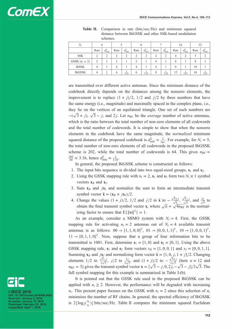
ntÞc bits/sec/Hz. Table II compares the minimum squared Euclidean

Table II. Comparison in rate (bits/sec/Hz) and minimum squareddistance between BiGSSK and other SSK-based modulationschemes.

Nt 4 5 6 7 16 32

Rate d2min Rate d2min Rate d2min Rate d2min Rate d2min Rate d2min

SSK 2 2 2 2 2 2 2 2 4 2 5 2

GSSK (nt ¼ 2) 2 1 3 1 3 1 4 1 6 1 8 1

BiSSK 4 1 4 1 4 1 4 1 8 1 10 1

BiGSSK 4 23

6 23:16 6 2

3:16 8 23:38 12 2

3:67 16 23:83


112


distances along with the transmission rates between BiGSSK and other SSK-based

modulation schemes.

4 Numerical results

For all the BER simulation results versus the average SNR per bit per receive

antenna (Eb=N0) presented in this section, Nr ¼ 3 receive antennas are employed.

The BERs of BiSSK and BiGSSK with different system settings are shown in

Fig. 1-(a). At fixed target transmission rates of 6, 8 and 10 bits/sec/Hz, BiGSSK

shows a negligible performance loss (<0:5 dB) but requiring much smaller numbers

of available transmit antennas as compared to BiSSK (e.g. for 10 bits/sec/Hz,

BiGSSK requires 9 antennas while BiSSK needs 32 antennas). With similar

numbers of transmit antennas, the transmission rate of BiGSSK(7,3) is higher, by

2 bits/sec/Hz (which is 33.33% higher), than that of BiSSK(8,3) at the expense of

1 dB performance loss at the BER level of 10�5.Comparison of LSSK(5,3) and BiGSSK(5,3) for the same number of transmit

antennas are shown in Fig. 1-(b). Both LSSK and BiGSSK schemes aim to enhance

the transmission rate of SSK under a limited number of transmit antennas. As can be

seen, although BiGSSK is inferior to LSSK by less than 0.5 dB, BiGSSK achieves a

significantly higher transmission rate (more than 2 bits/sec/Hz, or 50% higher) than

LSSK. The performance difference observed in Fig. 1-(b) can be roughly predicted

from the minimum squared distances in Table II and the spectral efficiencies of

BiGSSK (� ¼ 6 bits/sec/Hz) and LSSK (� ¼ 6 bits/sec/Hz) as follows. Since Es ¼�Eb, the power loss of BiGSSK compared to LSSK is 10 log10

6� 23:16

4�1 � �0:23 dB.This is reasonably close to −0.5 dB observed in Fig. 1-(b).

5 Conclusion

A new SSK-based modulation scheme is proposed by multiplexing in-phase and

quadrature GSSK streams and optimizing the signals transmitted over active

antennas. Given the same number of transmit antennas, the proposed scheme

doubles the transmission rate of GSSK and it achieves a higher transmission rate

than BiSSK at a negligible performance loss. Viewed differently, at the same

transmission rate, the proposed scheme employs a smaller number of transmit

antennas, leading to a reduction in hardware cost.

(a) BiGSSK versus BiSSK (b) BiGSSK versus LSSK

Fig. 1. BER comparison of BiGSSK with BiSSK and LSSK fordifferent ðNt; NrÞ.


113


Millimeter-wave closeproximity high-speed datatransfer system

Tadao Nakagawa1a), Hideki Toshinaga1, Toshimitsu Tsubaki1,Tomohiro Seki2, and Masashi Shimizu11 NTT Network Innovation Laboratories, NTT Corporation,

Yokosuka, Kanagawa 239–0847, Japan2 College of Industrial Technology, Nihon University,

1–2–1 Izumicho, Narashino, Chiba 275–8575, Japan


Abstract: This paper presents the system concept, transceiver architecture,

and control sequence for a millimeter-wave (60-GHz) band close proximity

high-speed data transfer system. The communication range and the use case

are limited to achieve fast link setup time and a stable point-to-point

connection. Prototype equipment developed for the system includes three

types of wireless transceivers; cooperative operation among them makes it

possible to reduce the link setup time and limit the communication range.

The system’s control sequence enables the link setup time to be reduced from

7 seconds to 0.2 seconds.

Keywords: millimeter wave, 60GHz, close proximity high-speed data

transfer, link setup time, point-to-point connection

Classification: Wireless Communication Technologies

References

[1] E. Perahia, C. Cordeiro, M. Park, and L. L. Yang, “IEEE 802.11ad: defining thenext generation multi-Gbps Wi-Fi,” Proc. IEEE 2010 Consumer Communica-tions and Networking Conference (CCNC 2010), pp. 1–5, 2010. DOI:10.1109/CCNC.2010.5421713

[2] T. Baykas, C.-S. Sum, Z. Lan, J. Wang, M. A. Rahman, H. Harada, and S. Kato,“IEEE 802.15.3c: the first IEEE wireless standard for data rates over 1Gb/s,”IEEE Commun. Mag., vol. 49, pp. 114–121, Jul. 2011. DOI:10.1109/MCOM.2011.5936164

1 Introduction

Mobile traffic has increased significantly in recent years with the widespread use of

smartphones and tablets and their increasingly high volume content. It is expected

that wireless LANs will enable traffic offloading, but in urban areas their effective

throughput is rapidly degraded as the user number increases. Millimeter-wave

(60-GHz) band wireless systems have a wide bandwidth of about 9GHz and great

© IEICE 2016DOI: 10.1587/comex.2016XBL0003Received January 5, 2016Accepted February 2, 2016Publicized February 22, 2016Copyedited April 1, 2016

114


http://dx.doi.org/10.1109/CCNC.2010.5421713





http://dx.doi.org/10.1109/MCOM.2011.5936164




potential in terms of capacity [1, 2]. There are, however, some problems in using

the millimeter-wave band, including link setup time and communication topology.

We propose a millimeter-wave close proximity high-speed data transfer system to

solve these problems and to provide a comfortable data transmission service. In this

paper we describe the system concept, transceiver architecture, and the performance

of prototype equipment developed for the system.

2 System concept

The use case of our target system is high-speed data download/upload services that

are carried out at kiosk terminals, which are located in many types of public spaces

including convenience stores, train stations, and airports. Our target system has the

following features:

1) Link setup time is less than 1 second:

Link setup includes association and authentication between a kiosk terminal and a

mobile terminal. When the transmission rate of wireless links becomes high, the

link setup time will remain noticeably high. For example, a video file with a

viewing time of 1 hour that is compressed with a H.265 video compression

standard has a data size of about 400MB. This results in file download/upload

time of about 3.2 seconds at a transmission rate of 1Gbit/s, while the link setup

time of the existing millimeter-wave systems is generally more than 5 seconds.

Thus the link setup time should be reduced to provide a short file transfer period.

2) The communication range is less than 10 cm:

This short-range system ensures that the system’s communication topology is a

point-to-point connection, whereas the existing millimeter-wave systems including

IEEE 802.11ad and IEEE 802.15.3c may have point-to-multipoint connections

since their communication ranges are several meters [1, 2]. A point-to-point

connection has a larger effective throughput than point-to-multipoint connections.

The effective throughput of user terminals at an access point or a base station

lessens as the number of users per cell increases.

In order to achieve these features, the system we propose combines multiple

wireless systems. We hereafter refer to it as the “proposed multiple wireless

system” and describe it in the following section.

3 Configuration

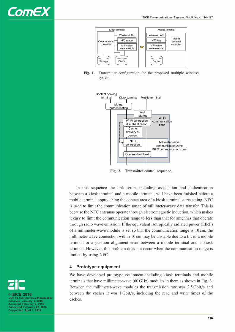
The transmitter configuration for our proposed multiple wireless system is shown in

Fig. 1. The kiosk terminals and mobile terminals have high-speed caches between

which data transfer is carried out. Both the kiosk terminals and mobile terminals

have three kinds of wireless transceivers: millimeter-wave, Wi-Fi wireless LAN,

and NFC (near field communications).

The transmitter control sequence is shown in Fig. 2. When a user with a mobile

terminal enters a Wi-Fi communication zone (about 10m), Wi-Fi connection and

authentication are carried out. The authentication information is used in millimeter-

wave connections and NFC connections. When a mobile terminal enters an NFC

communication zone (about 10 cm), the terminal is identified. Millimeter-wave data

transfer is carried out for the identified mobile terminals.


115


In this sequence the link setup, including association and authentication

between a kiosk terminal and a mobile terminal, will have been finished before a

mobile terminal approaching the contact area of a kiosk terminal starts acting. NFC

is used to limit the communication range of millimeter-wave data transfer. This is

because the NFC antennas operate through electromagnetic induction, which makes

it easy to limit the communication range to less than that for antennas that operate

through radio wave emission. If the equivalent isotropically radiated power (EIRP)

of a millimeter-wave module is set so that the communication range is 10 cm, the

millimeter-wave connection within 10 cm may be unstable due to a tilt of a mobile

terminal or a position alignment error between a mobile terminal and a kiosk

terminal. However, this problem does not occur when the communication range is

limited by using NFC.

4 Prototype equipment

We have developed prototype equipment including kiosk terminals and mobile

terminals that have millimeter-wave (60GHz) modules in them as shown in Fig. 3.

Between the millimeter-wave modules the transmission rate was 2.5Gbit/s and

between the caches it was 1Gbit/s, including the read and write times of the

caches.

Fig. 1. Transmitter configuration for the proposed multiple wirelesssystem.

Fig. 2. Transmitter control sequence.


116


Measured performance comparison between a conventional millimeter-wave

module (i.e., one for millimeter waves only) and the proposed multiple wireless

system is as follows:

1) Conventional millimeter-wave module:

The link setup time is 7 seconds. The communication range is 50 cm.

2) Proposed multiple wireless system:

The link setup time is 0.2 seconds. The communication range is 10 cm.

As the comparison shows, the latter has much faster link setup time at the

designed lower communication range.

5 Conclusion

In this paper, we described the system concept, transceiver architecture, and control

sequence for a millimeter-wave (60-GHz) band close proximity high-speed data

transfer system. The communication range and the use case are limited to achieve

fast link setup time and a stable point-to-point connection. Prototype equipment

developed for the system includes three kinds of wireless transceivers, and

cooperative operation among them makes it possible to reduce the link setup time

and limit the communication range. The system’s control sequence provided

1Gbit/s transmission rate and enabled the link setup time to be reduced from 7

seconds to 0.2 seconds with the targeted communication range of 10 cm.

Fig. 3. Prototype equipment for the proposed multiple wireless system.


117


Date post:	01-Mar-2021
Category:	Documents
Upload:	others
View:	1 times
Download:	0 times

IEICE Communications Express, Vol.5, No.4, 95 Synchronization … · 2016. 3. 28. · Abstract: The...

Documents