' 1 itrtl from AMEItICAS SCII~~STIS'I', Yol. 49, Xo. :l,, Sc. ~ t c nl r 4 1 rTT-- In.rp4 A t. f i g l $ ~ ~ ) TURBULENT FL@W;& F ; ~ ~ & \ I G N E E R I : - .

I,,-y or C A ~ ~ ~ G ~ ~ ' J ! A , BERKELEY by S. C O R R & & ~ ; ~ ~ ~ , ~ A m x f i I * 94720

M OST of the liquids and gases in the universe are in disorderly mo- tion. Combined with a general flow pattern there is usually a com-

plex random motion that we call "turbulence," which is not directly associated with the thermal agitation of the individual molecules.

Turbulence is especially likely to occur on geo- and astro-physical scales. On the human scale there are many flows without appreciable tnrbulence, the "iaminarJJ flows. For example, the water flowing a t 2 or 3 feet, per sccond in a %-inch tube has a smooth, glassy look, as it comes out the end (Fig. la). At a higher speed, however, the irregular (turbu- d'

leitt) motion makes its appearance (Fig. 1 ~ ) . The buoyant Convection above a cigarette is laminar for some distance before becoming turbulent (Fig. 2). You can easily discover that this distance gets shorter as ex-

it can be described ar Figure 3 is a

stabre) tube flow was laminar, but becomes turbulent shortly thereafter. Figure 4 shows a turbulent wake r3:.

On s larger scale, Figure 5 shows the effect of turbulent wind in the dispersal of smoke from a stack 141. The randomness of a sea surface (Fig. 6) may arise directly from the turbulence in the wind, or from surface interactions of wind and water flow. On a still larger scale, the Great Nebula in Orion (Fig. 7) looks rather like a turbulent puff of smoke. Turbulence is playing an increasing role in astrophysical theories 151.

In later sections, we look a t a few basic features of turbulence dy- namics, and a t some of its effects in mixing and dispersion. At present, we have a qualitative understanding of the phenomenon, and can even predict some of its features quantitatively from Newton's Laws. But much of the core o: the turbulence problem has yet to yield to formal theodtical attack.

Fluid Mechanics

Restricting ourselves to continuous media and to flows with speeds much smaller than that of light, fluid mechanics is the application of I

Newton's Laws to the motion of fluids under adequate initial conditions ? and/or boundary conditions. The Newtonian mechanics of one or two "mass pointsJ' or rigid bodies presents no great analytical difficulties

300 - . . 2 '

.-A - - F-- - --- --- TURBULENT FLOW

' ' P Q - 30 1

unless ve( ~ p l i c a t e d force fields are involved. For example, s two-

I .' body probiL?a has only twelve possible basic modes of motion. But a 1 .

deformable continuum has an infinite number of such "degrees-of-free- dom." Instead of merely a smalTin7E~rZI ni imEG3 v<IGity h i s G i G t o predict, we have the evolution of a full velocity jiekl. The expression of Newton's Second Law is therefore a partial differential equation w.

Field problems with their partial differential equations have presented no great obstacle to applied mathematicians as long as the equations and boundary conditions were linear. The history of successful analysis of

Fro. la. Laminar jet of FIG. 1 ~ . Turbulent jet of water. water.

From an article by the author in Johns Hopkins Magazine. Photographs by Werner Wolff-Black Star

problems in potential theory, simple wave motion and diffusion problems 171 goes back well oc-er a century.

Unfortunately, the espression of Newton's Law for fluid motion is non-linear, and we have no general soiution. Instead, each problem must be pursued more or less as a special case. Nevertheless, a large number of laminar $ow cases have been successfully studied, both analytically and in the laboratory.

I n a "&~ed" reference frame, Newton's Second Law is expressible as 181:

a Net force per '4 + C uk 2 = at k - I fluid "element" 1

4

Acceleration of fluid "element"

302 . AMERICAN SCIENTIST f where i = 1, 2 or 3 correspond to components in the thk (orthogonal) Cartesian directions. U is velocity vector, xis coordinate vector, 1 is time. In this form (1) applies to solid materials as well as fluids.

Equation (1) is in a "fixed Eulerian frame"; X I , x2, xl, the components of x, are definite space coordinates. In this frame the "convective ac-

Fro. 2. Free convection plume above cigarette. The laminar jet Reynolds number increases upward (from nn article by the author in Johns Hopkina Magazine). Pho-

tograph by Werner WOW-Black Star

celeration" terms are non-linear, being quadratic in the dependent variable, the velocity.

The s imples t l i s t i c mathematical m e - - - ----______-__ model for force @ue to interac- tions with the rest of the fluid) is the "Newtonian Fluid,"@ch has ------ ---- -- .. * - .--. just a simple proport=litybetween shear stress and distortion rate. -- Then, restricting to constant viscosity IJ, (1) has the form r e ~ :

v = pip, the "kinematic viscosity"; p is static pressure;' p is density. The fact that matter is neithcr created nor destroyed is expressed by

. * . . . iT TURBULENT FLOW

the ''con( ty equation,"

Equations (2) and (3) are found to give an accurate description of a great many important fluid motions, for example, air flows a t speeds below about 200 ft./sec. and water flows up to still higher speeds if

FIG. 3. Forced convection (blown) jet (from an article by the author in Johm Hop* Magazine). Photograph by Werner Wolff-Black Star .

there is no "cavitation." If density variations, gravity forces and steady . rotation of the coordinate system are added, these equations describe

the motion of nearly the entire atmosphere and ocean systems.

The Theoretical Turbulence Problem The analytical study of turbulent flow can now be described as the

attempt to predict the history of a random (velocity) field whose be- haviour a t each point in space-time is given by equations (2) and (3).

Since the flow is random, we work in statistical mechanics, seeking not an explicit account of the motion of every particle of fluid, but only a

1 304 AMERICAN SCIENTIST / '

I

statistical description in terms of various averaged f u n d .. Simplest of these is the average velocitv distribution. More generally, we may re- quire some measures of the turbulent fluctuatio~~ intensity, the charac- t a d the vrobability . . (density) for the occurrence of A . n v v e l o c i t y or set of vdwties? etc.

Although the goals of a statistical mechanical analysis are thus more

Pro. 4. A pellet moving at supersonic speed shows a turbulent wake, along with an assortment of shock waves and a streamline made visible by a temperature jump. (Courtesy of Ballistic Research L&b, Aberdeeu Proving Ground.)

modest than those of deterministic mechanics, we pay a heavy penalty: our system of equations, (2) and (3), which is exactly determinate in the sense of having 4 equations for 4 unknown functions (U1, U2, Us, p; p and v are "given"), leads to systems of statistical equations which are v indeterminate. Any finitecollection oi -fewer in number a - e than cC.ec

~ ~ s i & ~ ~ a ~ f u 1 c ~ i 6 n f f i ~ ~ - ~ 6 i 3 ~ n r 181. This results from W t,-6-;i-nll L-n- a-r tlQ-6rxhF s-j,kteG *--- --- ----

- - - --- . _ _ _ .-

T F i G e f o F a f ; the heart of each theory of turbulent motion is one or more additional postulates relating some of these unknown statistical functions to eachother.

, . . . TURBULENT FLOW i 3 0 5 J I c The Turbulent Energy Spectrum T'

Prime target for most turbulence theories is prediction of the energy spectrum, a measure of hbw the . . . mi3EGpect to "eddy sizes." For this we choose a three-dimensional G r i e r representation, so thesimplest e l e m e a s a single ' @ i ?

r filling the entire physical space. In wave number sp%e (wave number = 2 r/wave length) this s ane element is a point vector value (Fig. 8).

A statistically homogeneous field of turbulence is thus representable as an infinite collection of such "shear wavesJJ in physical space (con- tinuously distributed in wave length and orientation), or a corresponding collection of point vectors in wave number space. Because of the non- linearity of the NavierStokes equations, these Fourier elements are in continuous interaction.

. . - .--_I- ---- . .

FIG. 5. Dispersion from a emoke stack (from motion picture "Turbulent Flow," The Johns Hopkine University, 1957).

The simplest measure of spectral distribution is the relative integral "intensityJ' of these point vectors a t any radial distance k from the wave number origin. This is called the "three-dimensional spectrum," and i t does not distinguish directions of nodal planes or velocity vectors. It has a form qualitatively like Figure 9. I t s integral is just the total turbu-

Here *ul, ~ 2 , 7 1 3 are Cartesian components of turbulent velocity. The over- bar denotes average value. Of course & may depend on time t.

A differential equation for &(k, t) may be deduced from Newton's Law, equation (1):

306 AMERICAN SCIENTIST

FIG. 6. Irre~dar wave pattern on the sea surface is associated with turbulence (courtesy of U. S. Navy Hydrographic Service).

The terms represent (a) the time rate of change of turbulent energy associated with wave number k, which results from the net unbalance of two effects: (b) the rate of viscous dissipation of turbulent energy a t k (directly to interiial energy of the molecules) and (c) the net rate of gain of energy a t k due to (non-linear) interactions with a11 other Fourier components.

Since (5) is a siugle equation with two unknown fu~ctions, i t is inde- terminate. The simpler turbulence theories use this as their basic equa- tion, eliminating r by introducing postulates for expressing it as some function of &. Some of these theories have had limited success.

In the statistical mechanics of discrete psrticles, the prime theoretical target is not a function analogous to &, but rather the simple probability densities (usually called "distributions" by physicists), the relative likelihood of occurrence of each value of velocity. These probability densities are also interesting in turbulence and have been measured, but no tractable differelltin1 equations for them have yet been deduced.

Non-Linearity and Spectral Transfer

The heart of the turbulence spectrum prohiem is the-nature of the intrraction function IYk. 1) in eauation (5:. I t depends on the sum of

.. . . . TURBULENT n o w 307 . - averaged t( of Fourier elements. The fact that a non-linear

- system must have such spectral interaction can be seen from the response of a much simpler non-linear system, an "instantaneous" device whose input-vs.-output curve is not a straight line. Figure 10 illustrates the effect with an input whose spectrum is a single "Fourier point," i.e., a purely sinusoidsl signal. In general, the output contains all "higher harmonics." This particular non-linear device evidently feeds energy from lower to higher frequencies.

I t appears that non-linearity generally tends to shift spectral content

Fra. 7. The Great Nebula in Orion (Mt. Wilaon Observa- tory 1.

from lower wave numbers (or frequencies) to higher ones, although some :ocalized esceptions have been found. In a turbulent flow, the energy path in xave number space can be crudely represented as in Figure 11, nith nn "energy cascade" proceeding from larger to smaller eddies, . . Figure 12 is more esplicit. Theturbulence receives rts e n e r ~ s e ">,

mean flow (also by courtesv of the n-itv of the equations of motion) when there is a mean velocity gradient., -From a geometrical viewpoint, the spectral transfer process in turbu- i

lence can be seen in the (empirical) fact that any blob of fluid momen- '\, tarily having a fairly uniform local velocity, is stretched and twisted by it.s own motion (and that of neighboring fluid) into ever longer, thinner 1 and more convoluted "strings" and "sheets." Since i t is difficult to sketch '

such a locally coherent velocity field, we can illustrate this aspect via a

AblERICAN SCIENTIST

I W a v e number space Physical space

FIG. 8. A single Fourier element of velocity field (from Jour. Ceophys. Res.).

- I k. i- inertial and 1

- I

' isatrooic k' --- purely inertial ' maxed ~nerttol [6?(k9.)

and viscous

FIG. 9. Three-dimeneional turbulent energy spectrum and dissipation spectrum. k* corresponds to the "J<olmogorov microscale, mentioned in the concluding section (from Jmrr. Geophys. Rrs. Dec., 1959).

similar pheuomenou: turbulellt mixing of n passive scalar contaminant, like dye spots, in a turbillent liquid.

Turbulent Mixing

011e of the most familiar actions of turbulo~t motion is its effective- ness ill mixing up two ingredients, such :LS cream and coffee. This phe- nomenon is seen most clearly by eliminating molecular mixing, an act which is easier to think of (Fig. 13) than to perform in the laboratory.

In this sketch the distortion is performed mostly by turbulent "ed-

TURBULENT n o w

I

Input

(a1 linear device $- input signal

(b) non-linear device:

Oulpul conlainr higher harmonics

input siqnal

ha. 10. Illustration of spectral transfer due to non-linearity. The output of the linear device contains only the single input frequency (from Jout. Geophya. Res., Dec., 1953).

Distibuted energy inflow I from mean motion

I I

i

Meon flow

kinetic

~ W Y

Fto. 12. Schematic representation of average turbulent kinetic energy path in wave number space

+

furbulenl Turbulent infernal

kinetic kine& energy e'"WY e"WY of fluid

( l o g e eddies) (small eddies) ( h e a t i h

Turbulent energy flow

AMERICAN SCIENTIST /- - f '

Fra. 11. Crude representation of average energy degradation path

rote through any value of wave number

a. Binary distribution in space ( +

Rough spectral location

- ---+ --+

b. Amplitude on a cut

El to m tl ' to t. > tl

c Effect of molecular transport for t >to

- Rough spectral locotion of energy

inflow or 'production" Distributed outflow (dissipation) t o heat

FIG. 13. Schematic sketch of turbulent mixing of a contaminant, both without and with molecular diffusion. These represent a small sample from a large statistically homogeneous field.

FIG. 14. Schematic sketch of turbulent distortion of a spot of contaminant much smaller than the turbulent "eddies."

dies" which are smaller than the original blob of dye. I t is obvious that rr spatial Fourier analysis of dye concentration here mill show a flux from low to high wave numbers in the spectrum UII. The effect of molecular diffusion is added in part (c). We see how the random turbulent convec- tion, by tending to increase local concentration gradients, hastens the approach to molecular homogeneity. i

Parenthetically, Figure 13a suggests the usefulness of turbulence in

312 AMERICAN SCIENTIST 1 J making emulsions. If there were surface tension betweal the st+kd and

unshaded fluid, small drops would be pinclied ofl. Although Figure 13 illustrates the spcctral cascade contribution made

by turbulence structure which is smaller than the dye blob, eddies of all sizes contribute. Figure 14, for example, indicates thc fate of a similar spot under the action of eddies much larger than itself. Obviously, the spectral content has gonc to lower wave numbers for one particular spatial direction, but, when me average over-all clircctio~~s; thc net spectral shift is again toward h i g h wave numlm-s

The relative rates of approach to nlolecular homogeneity is very much faster with turbulence to assist. Figure 15 shows parallel photographic

FIG. 16. Small sections of typical grids used to generate approximntrly isotropic turbulence for experimental research.

time sequences from two mixing experiments with the same mixer speed; The left-hand sequence has high enough Reynolds number for the occ~lr- rence of turbulence; t3he right-hand scqcence does not, and is thc~rciorc a laminar mixing operation 1121.

The problcm of scalar mixing by a (statistically) given turbulence field not only has immense practical importance; i t is also u logical step toward an ultimate underst.anding of the turbulence itself. I t is a linear problem under the fornlal mathematical definition: the concentrstion field has no effect.on itself as the turbulent velocity field does, and i t harbors no complicating phenomenon such as static pressure.

Tendcnci~s Toward Isotropy

It is found experimentally that roughly homogcncous turbulence which is receiving no furthcr energy from the meah flow tends'to I~ccomt: isotropic, i.e., its statistical properties tend to become thc same in all

3 - * . - ,l TURBULENT FLOW 313 /

t t ~ e c o y i n g n turbulence

\ \ \ \ \ \ \ \ \ \ \ \ \ \ \ \ \ \ \ *I 3 - - - - - It rr --- ----/y==--=- -

U n i f o r m 31 --->--* - - C _ - f l o w -- 3; - - - - --+z z-L-

31 - - - -- a; -- --y- - - r- G L P

' g r i d \ \ \ \ \ \

FIG. 17. Conventional method of generating approximately isotropic turbulence (from Jour. Geophys. Res., Dec., 1959).

'\transverse

\ '. '--. --% - --

t streomwise

IG. 18. R.m.8. turbulent velocity fluctuations during gross atrain and afterward (from Jour. Geophys. Res., Dec., 1959).

directions [ I ~ I . For example, a square-mesh grid (Fig. 16) set across a uniform flow is a very non-isotropic flow configuration (Fig. 17). Yet, sorne 40 to 50 mesh lengths downstream, the turbulence it generates is roughly isotropic. Of course, the turbulent energy is also decaying toward zero because ~f viscous dissipation.

h more well-defined experiment on the tendency toward isotropy is to send this roughly isotropic field through a duct contraction. The preferential distortion induces a strong anisotropy. Yet, as indicated in Figure 18, the mean-square turbulent velocity components approach equality inslater uniform flow region.

C -- - - -

Xt &n be shown analytically that this intercomponent energy trardfgp depends a t least partly on the static pressure fluctuations. This is not too

I 7-\ 314 AMERICAN SCIENTIST

FIG. 19. Tendency of dye stripes toward atatistical isotropy as a result of turbulent con- vection (from motion picture "Turbulent Flow," The Johns Hopkins University, 1957).

I surprising since pressure is a scalar quantity, but up to now there is no theory that predicts even the sign of the transfer.

No doubt the tendency of a homogeneous, isolated turbulence toward . I

isotropy is an instance of a general tendency towdrd equipartition en- countered also in more traditional problems of statistical mechanics.

A parallel, but not analogous, approach toward isotropy is seen ia

. * /-%, TURBULENT FLOW

a n o t h e r ~igeneous turbulent mixing problem. If we have a fluid in roughly isotropic turbulent motion, and introduce strongly oriented (hence, anisotropic) streaks of dye, we find the streaks getting more and more convoluted in a way which makes the dye cbncentration field ap- proach an isotropic state (Fig. 19).

A rather different aspect of the approach toward encrgy equipartition in turbulence dynamics is the phenomenon of 'tlocal isotropy." Rven _--- though the large structure of a turbulence field may have preferred - directions, the fine structure (the "small eddies") may be isotropic. - The theoretical postulate [MI, based on the idea that the non-linear - spectral energy cascade is an orientation-losing process, has received some experimental support when the Rcynolds number is sufficiently large..

. Reynolds Number and Spectral Form

At this point, some remarks on Reynolds number are relevant. From the Savier-Stokes equations, it can be shown that a basic dimensionless parameter in viscous flow is thc ratio of the magnitudes of "inertia forces" (a pseudonym for accelerations) to viscous shear forces. This ratio is called the Reynolds number. For h e d system geometry it turns out to be

where D and U are characteristic length and mean velocity respectively; v is kinematic viscosity.

In homogeneous turbulence there are no characteristic mean flow velocities or lengths, so a11 appropriate Reynolds number can only be made up with statistically defined turbulence parameters.

For example, we may use

where u' is a root-mean-square turbulent velocity component and L is an "average eddy size1' computed from the energy spectrum r151.

It is helpful to introduce thehotion of q spectral Reynolds number, m(!c), to characterize the ratio of inertial to viscous effects for the eddies of different sizes. From d;mensional reasoning i t can be seen that a length characteristic of the sgectral domain of wave number k is just its in- verse,

[lei, while a velocity characteristic of this part of the spectrum function is

vr lk&(k)]"' (9)

AAIEHICAN SCIENTIST

Fxa. 20. Experimental turbulence spectrum. The straight line hrrs slope -%. corresponding to equation (12).

Since &(k) itself must decrease a t large k (because its integral, the tur- bulent energy, must be finite), m(k) must decrease. I t follows that for ?ma11 enough eddies the viscous forces must be important.

One of the simplest, and probably most enduring parts of contem- po:ary turbu!ence theory is liolmogorov's prediction of the form of &(k) over a limited range where thcre is local isotropy (so that i t must hzxe k >> ] / I , ) and where @(k) >> 1. For this "inertial, isotropic range;" he postulated that the local form of the energy spectrum depends ortly on the total rate of energy flux from wave numbers less than k to wave numbcrs larger than k. Since @(k) is very large, and is presumably still !arger a t lower wave numbers, a11 viscous dissipation occurs a t k values beyond this spectral range (see Fig. 12). Therefore, the-rate of flu through this k must just equal the total rate of viscous dissipation 4:

X Measurements '*, (x/M = 16. UM/3=9600)

', --- Normal distribution

\

Probability density function of u,.

FIG. 21. Comparison between measured probability density of velocity in turbulence and a Gaussian ("normal") density. M is grid mesh, X is distance be- hind grid.

o Measurements (x /M-25. UM/3=38x103

___Normal d~str~bvt~on wtth the same standard devlat~on

Probability density function of tub12x,.

Fro. 22. Comparison between measured probability density of velocity derivative and a Gaussian density.

according to equation (5). This also shows the dimensions of 4. The only form dimensionally possible is found to be

This result, generally accepted as likely since i t became widely known, is just beginning to receive firm experimental confirmation

a (Fig. 20) 1171. The most successful theories for the form of &(k) outside the isotropic

inertial range are immensely more complicated than the foregoing. The (small structure) viscous domain is beginning to yield to study and ex- periment. A spectral transfer theory of Heisenberg rial is based on the

318 AMERICAN SCIENTIST f --- introduction of a small-eddy "turbulent viscosity" into the ,&) term of

equation (5), to change i t superficially into a form like the (b) term. His asymptotic prediction, fork -+ is

This is not a t serious variance with experiment, a t least for a k-range just above that appropriate to (12). The implied non-existence of higher moments of &(k) is, however, worrisome, and Townsend tior now offers theoretical and experimental hope for an exponential tail on the spec- trum.

, relative

Typical members of I * the "ensemble" of trials Collective plot

of o few trials ~ s ~ r n ~ t o t i C result

fu on rn number d trials

FIG. 23. Schematic sketch of turbulent dispersion from a "point source" in time t.

Probability Densities

In a process as inherently non-linear as isotropic turbulence, we might expect the probability densities of the velocity components to be rather lopsided. Figure 10 shows how a non-linear device can convert a sym- metric signal to an unsymmetric one. Experiment shows the surprising fact that the densities of velocities in grid turbulence zre Gaussian within,) the limits of accuracy (Fig. 31) 1201. The spatial velocity derivatives, however, do show considerable "skewness" (Fig. 22) [POI. It can be de- duced by formal analysis that this skewness is intimately related to the . (non-linear) spectral energy transport. The higher derivatives are even farther from Gaussian 1211 .

Theoretical predictions of the important probability density function

TURBULENT FLOW 319

in I?& i2 are tlon-existent, but rough estimates of its skewness have 9 .

< . been obtained.

The observed Gaussian character of velocity (and of particle displace- ment) may be simply the result of something like a "central limit theorem" 1221, in the sense that non-linear dynamic effects influence the acceleration directly, whereas the velocity is the integral (sum) of ac- celerations.

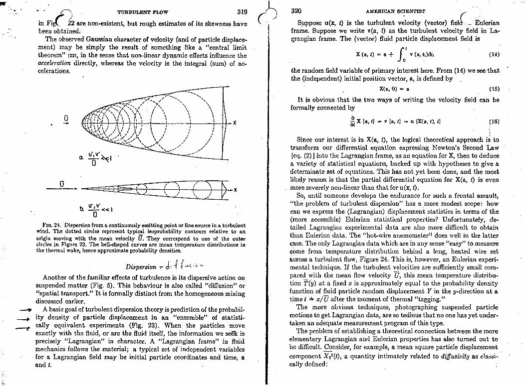
FIG. 24. Dispersion from a continuously emitting point or line source in a turbulent wind. The dotted circles represent typical isoprobability contours relative to an origin moving with the mean velocity 3. They correspond to one of the outer circles in Figure 23. The bell-shaped curves are mean temperature distributions in the thermal wake, hence approximate. probability densities.

Another of the familiar effects of turbulence is its dispersive action on suspended matter (Fig. 5). This behaviour is also called "diffusionJJ or "spatial transport." It is formally distinct from the homogeneous mixing discussed earlier.

4 A basic goal of turbulent dispersion theory is prediction of the probabil- - ity density of particle displacement in an "ensembleJ' of statisti-

-7 cally equivalent experiments (Fig. 23). When the particles move exactly with the fluid, or are the fluid itself, the information we s e a is precisely "Lagrangian" in character. A "Lagrangian frame" in fluid mechanics foIlows the material; a typical set of independent variables for a Lagrangian field may be initial particle coordinates and time, a and t.

320 AMERICAN SCIENTIST f Suppose u(x, t) is the turbulent velocity (vector) fiel&- -. Eulerian

frame. Suppose we write v(a, 2) as the turbulent velocity field in La- grangian frame. The (vector) fluid particle displacement field is

X (a, 1 ) = a + $: v (a, C M h (14)

the random field variable of primary interest here. From (14) we see that the (independent) initial position vector, a, is defined by .

I t is obvious that the two ways of writing the velocity field can be formally connected by

Since our interest is in X(a, t), the logical theoretical approach is to transform our differential equation expressing Kewton's Second Law [eq. (2)] into the Lagrangian frame, as an equation for X, then to deduce a variety of statistical equations, backed up with hypotheses to give a determinate set of equations. This has not yet been done, and the most likely reason is that the partial differential equation for X(a, t) is even more severely non-linear than that for u(x, t) .

So, until someone develops the endurance for such a frontal assault, "the problem of turbulent dispersion" has a more modest scope: how can we express the (Lagrangian) displacement statistics in terms of the (more accessible) Eulerian statistical properties? Unfortunately, de- tailed Lagrangian experimental data are also more difficult to obtain than Eulerian data. The "hot-wire anemometerlVoes well in the latter case. The only Lagrangian data which are in any sense "easy" to measure Qome from temperature distribution behind a long, heated wire set across a turbulent flow, Figure 24. This is, however, an Eulerian experi- mental technique. If the turbulent velocities are sufficiently small com- pared with the mean flow velocity u, this mean temperature distribu- tion T(y) a t a fixed x is approximately equal to the probability density function of fluid particle random displacement Y in the y-direction a t a time t A x/a after the moment of thermal "tagging."

The more obvious techniques, photographing suspended particle motions to get Lagrangian data, are so tedious that no one has yet under- taken an adequate measurement program of this type.

The problem of establishing a theoretical connection between the more elementary Lagrangian and Eulerian properties has also turned out to be difficult. Consider, for example, a mean square particle displacement component e(t), a quantity intimately related to digusioity as classi- cally defined :

TURBULENT FLOW

. . . . : 1 : I ; . . . . rtc. : I : I . Fro. 25. A few members of an infinite ensemble of realizations for a stationary random

variable 3(s), printed as D(') in the diagram.

From one component of equation (14)) Taylor (241 related this to a Lagrangian 'Lauto-correlation" function, &(a, 7, t ) =vz(a, t )v~(a + a, t + ~):[281

(where we choose a = 0, and have restricted to a single particle, a = 0). The overbar denotes alTerage value, "ensemble acerage" for theoretical sim- plicity. Equation (18) 1s restricted to statistically steady and homogene- ous turbulence. This relation was a big step forward because it showed precisely which Lagrangian velocity field function needs to be studied "

by people interested in diffusion. What kind of quantity is L ( 0 , T), viewed from our fixed (Eulerian) frame? We can write a formal expres- sion for i t in terms of the Eulerian component field uz(x, t) by referring to equation (1 6) :

Suppose the Eulerian correlation u4x, t)u2(x + €, t + 7). is known. This still doesn't enable us to calcuiate L2 because X is an unknown random trajectory through the random Eulerian velocity field. Up to now no one has found a unique connection between Eulerian and La- grangian correlation; in fact, i t can be shorn that a precise relation exists only a t the "functional" level, when we consider all the points together.

One aspect of the relation between the Lagrangian autocorrelation and the Eulerian field can be seen through the much simpler case of any single, scalar, stationary random variable 6(s), an abstract variable, not in a fluid flow.

Figure 25 represents the ensemble of realizations of this random vari- able by means of small segments of a few typical members. Let's think of this as an ensemble of Eulerian "fields." The classical autocorrelation function in this frame is gotten by the ensemble average, defined as folIows:

But suppose that the two-point separation length a, instead of being fixed, is made a random variable. As long as u is statistically independent- of r9., the correlation can be directly computed 1251. But suppose that the value of a to be used in each member of the ensemble depends analytically on the actual form of 6(s) in that member. Then the autocorrelation that results can be represented schematically by

The problem of this "self-dependent autocorrelation" in terms of the Eulerian statistical properties of 6(s) contains some of the flavor of our Euler 4' Lagrange problem.

Some Current Eflorts

Compared with some other branches of fluid mechanics, there is relatively little basic research going on in turbulence a t the moment, yet i t may be more than a t any time in the past. Probably not more than Mty people in the world are active in the field. This is in sharp contrast, for example, to the fascinating, fashionable and important new area of "magnetohydrodynamics" or "plasma dynamics," probably pursued by thousands.

Experimental basic research in turbulence is now aimed chiefly a t the following kinds of measurements:

1. The nature of laminar flow instability and the transition to turbu- lent flow.

" P TURBULENT FLOW 323

2. E .,,gy spectra a t higher Reynolds numbers. 3. Direct determination of the spectral transfer function. 4. Eulerian correlation functions for velocities a t points separated in

both space and time. 5. Details on the effects of turbulent motion in homogeneous mixing,

in dispersion and in sound scattering.

The next few years may see correlations and probability densities measured for three or four points in space-time. We shall want more in- formation on statistical properties of the velocity derivative fields, be- cause these seem more sensitive to the essential non-linearity of the phenomenon. Considerably more sophisticated Lagrangian data might be very stimulating, but are not too likely unless shortcuts can be de- vised, to avoid the tediousness of extracting data graphically from thousands of particle trajectory photographs.

Today's basic theoretical efforts are directed a t treating the triple Fourier component interactions which are a t the heart of the spectral transfer process. The older theories replace these essentially by double interactions, which cannot be correct in principle. Some encouraging anzlyses have already been published [ ~ G I .

The future of theoretical turbulence dynamics may depend on the successful use of "furctional analysis," although this path is still not clear. I t is also possible that theories for estimating Lagrangian func- tions in terms of Eulerian ones will need to make use of the same sort pf mathematical tools.

Sooner or later, serious prediction of probability density functions should be attempted.

In closing, we must certainly speculate on the future role of large computing n:achines in turbulence research. Valuable computations have already been made to illustrate the detailed predictions of exist- ing theories; these computations are doubtless too lengthy to have been undertaken by desk calculator. But a more exciting prospect lies in the use of very large machines to follow, directly, the consequences of the Savier-Stokes equations under random initial conditions. Primitive attempts were made some time ago, but the memory of even the latest generation of machines seems far too small for the job.

Imagine, for example, that we want to follow on a digital computer the details of decaying "turbulent flow" in a space of characteristic dimen- sion HI volume Ha. From experience we estimate an "average eddy size" L equal to roughly H/10. To simulate turbulence which has somede- gree of universality, we must insist on large Reynolds number, say RL = lo4 or larger. With this value it can be shown theoretically that the size of the "small eddie~" will be about

324 AMERICAN SCIENTIST

the "Kolmogorov microscale." This is the maximum allowab!e spacing for lattice points; actually there is significant flow structure which is smaller.

This requires 1012 points a t which three velocity components plus static pressure must be recorded in order to make each small time step. Further, if we want to resolve *50 different levels of each variable, es- sentially 4 X lOI4 points must be located by 'the memory. The number of "bits" of information is 2.7 X 1013, somewhat smaller because the level values of each quantity a t a point are mutually exclusive.

The foregoing estimate is enough to suggest the use of analog instead of digital computation; in particular, how about an analog consisting of a tank of water?

NOTES AND REFERENCES 1. The word "fluid" includes both gases and liquids. 2. For a recent t)iogr:rphical sketch, see Osborne Reynolds of Afanchester, Contribu-

tions of an Engineer to the Understanding of Cardiovascl~lar Sound, by V. A. McICusick and N. K. Wiskivtl, Btill. lfist. Med 5.9 (2), March/April, 1959.

4. This "shadomgraph" shows miex of refraction ~rregularities. I n the wake, these result from the irregularly distributed viscous dissipation (to interns1 energy) of the turbulent kinetic energy.

I. In this case the internal stack flow and the stack make also contribute to the turbulence.

5. See, for example, C. F. von Weizsacker, "The Evolution of Stars and Galazies," Astrophys. Jour., 114 (2), Sept. 1951.

6. This is the logical limit of a collection of simr~ltnneous total differential equations reprrsrnting Newton's Law for the collection of particles that makes up the rontinuum.

7. Inclrlding heat conduction. 8. This is expressed in the "Euleriun" frame (after the mathematician L. Euler).

An alternative fmme, in which we follow the material points of the continuum, is called "Lagrangian" (after J. Lagrange) and can give a linear form to the ac- relcrntion term; unfortunstelv, i t then yields a very complicated non-linear form for the force term in the simplest (Newtonian) viscous fluid.

9. This set of 3 equations is usually referred to as the Navier-Stokes equations. 10. Except possibly a t the level of "fnnctionals." See E. Hopf, Slatistical Hydro-

mechanics and Functional Culculus, Jour. Rat. Mech., 1 (I), 1952. 11. It is interesting to note that the dye concentration equation is formally linear:

I t shows some quasi-non-linear behaviour because the "forcing function" (the convective velocity field Ui) multiplies the dependent variable.

12. The A, B, C, D sequence is ordinary coflee and cream; the E, PI G, H sequence is molasses with "thick" white paint. The much higher latter viscosity yields a much lower Reynolds number, although characteristic size and speed are equal.

13. The theoretical concept of isotropic turbulence, the simplest type, was introduced by G. I. Taylor: "Statistical Theory of Turbulence," Proc. Roy. Soc., A, 161, p. 421 1193.5).

14. conEept d u e to A. N. Kolmogorov, "The Local Structure of,,Turbu[ence in In- compressible Viscous Fluid for Very Large Reynolds Numbers, C. R. Akad. Sci. U.R.S.S. (Doklady), $0, p. 301 (1941).

15. For example, L may be the integral of a spatial auto-correlation function of the turbulent velocity field.

16. Of course, the actual Fourier wave length is 2 r/k, but the 2 r factor is simply a constant, end there is no particular reason to use exactly the wave length. For instance, the characteristic width of monotonic shear is a quarter wave length.

17. For the most persuasive experimental confirmation, a t high enough Reynolds

TURBULENT FLOW

number, see H. L. Grant, A. Moilliet, and R. W. Stewart, " A ~ p k .m of Turbu- lence at Very High Reynolds Number," Ndure, 811, p. 808 (1959).

18. W. Heisenberg, "Zur Stalistwchen Thwric der Turbulenz," Zeils. Physik, I%$, p. 628 1194R\. --- \----,-

19. A. A. Townsend, "On the Fine-Scale Slrudurc of Turbulence." Proc. Rov. Soe.. A. . . $08, p. 534 (195i).

20. G. K. Batchelor, I'he Theory of Homogeneous Turbulence, Cambridge Univ. Presa, 1953 [page 1731.

21. G. I<. Batchelor,and A. A. Townsend, "The Nature of Turbulmf Motion at Large Wave-Numbers, Proc. Roy. Soc., A , 199, p. 238 (1949).

22. Central limit theorems are a class ~ r o v i n a that verv larae sums of small random "eventa" tend to become Gaussian' undeFcertain r&tri&ons, even when the in- dividual events ore not Gaussian.

23. See, for example, L. S. G. Kovasznay, "Turbulence hleasuremenb," Section F, Vol. I X , High Speed Aerodynamics and Jet Propulsion, Princeton Univ. Press, 1954.

24. G . I. Taylor, "Theory of Digusion by Continuous fovemenls," Proc. London Malh. Soc., $0, p. 196 (1921). T h e form in (18) is d f e t o J . Kamp6 de Feriet.

25. I t is just the probability-weighted integral of the "Eulerian" autocorrelntion. 26. See, for example, J. Proudman and W. H . Reid, "On the Decay of a Normally Dls-

tribufed and Homogeneous Turbulenl Velocity Field," Phil. Trans. Roy. Soc., A, 247, p. 926 (Nov. 1954); T. Tatsumi. "The Theory of Decay Process of Incom- presible Isotropic Turbulence," Proc. Roy. Soc., A, 239, p. 16 (1957); R. H . Kraich- nan, "The Structure of Isotropic Turbulence at Very Ifigh Reynolds Number," Jour. Fluid Mech., 6 (4), 1959.

27. 9 is just the inverse of the k* rn Figure 9. 28. Professor J . L. Lumley h m shown (private communication) that the two-parti-

cle Logrongian velocity correlation in a homogeneous, stationary turbulence must depend on time t as well as on time difference, 7.