83


ii
REPORT DOCUMENTATION PAGE
Form approved OMB No.
Public reporting for this collection of information is estimated to average 1 hour per response, including the time for reviewing instructions, searching existing data sources, gathering and
maintaining the data needed, and completing and reviewing the collection of information. Send comments regarding this burden estimate or any other aspect of this collection of information,
including suggestion for reducing this burden to Washington Headquarters Services, Directorate for Information Operations and Reports, 1215 Jefferson Davis Highway, Suite 1204, Arlington,
VA 22202-4302, and to the Office of Management and Budget, Paperwork Reduction Project (0704-1833), Washington, DC 20503
1. AGENCY USE ONLY (LEAVE BLANK)
2. REPORT DATE
12/2015
3. REPORT TYPE AND DATES COVERED
Final Report: 05/2014 – 12/2015
4. TITLE AND SUBTITLE
Transportation Life Cycle Assessment (LCA) Synthesis:
Life Cycle Assessment Learning Module Series
5. FUNDING NUMBERS
101412
6. AUTHOR(S)
Liv Haselbach, Associate Professor, Washington State University
Quinn Langfitt, PhD Student, Washington State University 7. PERFORMING ORGANIZATION NAME(S) AND ADDRESS(ES)
Department of Civil and Environmental Engineering
Washington State University
PO Box 642910
Pullman, WA 99164-2910
8. PERFORMING ORGANIZATION REPORT
NUMBER
9. SPONSORING/MONITORING AGENCY NAME(S) AND ADDRESS(ES)
Center for Environmentally Sustainable Transportation in Cold Climates
University of Alaska Fairbanks
Duckering Building Room 245
P.O. Box 755900
Fairbanks, AK 99775-5900
10. SPONSORING/MONITORING AGENCY REPORT NUMBER
11. SUPPLENMENTARY NOTES
12a. DISTRIBUTION / AVAILABILITY STATEMENT
No restrictions
12b. DISTRIBUTION CODE
13. ABSTRACT (Maximum 200 words) The Life Cycle Assessment Learning Module Series is a set of narrated, self-advancing slideshows on
various topics related to environmental life cycle assessment (LCA). This research project produced the first 27 of such modules, which
are freely available for download on the CESTiCC website http://cem.uaf.edu/cesticc/publications/lca.aspx. Each module is roughly 15-
20 minutes in length and is intended for various uses such as course components, as the main lecture material in a dedicated LCA
course, or for independent learning in support of research projects. The series is organized into four overall topical areas, each of which
contain a group of overview modules and a group of detailed modules. The A and α groups cover the international standards that define
LCA. The B and β groups focus on environmental impact categories. The G and γ groups identify software tools for LCA and provide
some tutorials for their use. The T and τ groups introduce topics of interest in the field of transportation LCA. This includes overviews
of how LCA is frequently applied in that sector, literature reviews, specific considerations, and software tutorials. Future modules in this
category will feature methodological developments and case studies specific to the transportation sector.
14- KEYWORDS : Please be sure they are searchable in the Transportation Research Thesaurus
http://trt.trb.org/trt.asp? Life cycle analysis, environmental impacts
15. NUMBER OF PAGES
74
16. PRICE CODE
N/A 17. SECURITY CLASSIFICATION OF
REPORT
Unclassified
18. SECURITY CLASSIFICATION
OF THIS PAGE
Unclassified
19. SECURITY CLASSIFICATION
OF ABSTRACT
Unclassified
20. LIMITATION OF ABSTRACT
N/A
NSN 7540-01-280-5500 STANDARD FORM 298 (Rev. 2-98) Prescribed by ANSI Std. 239-18 298-1

iii
Disclaimer
This document is disseminated under the sponsorship of the U.S. Department of Transportation
in the interest of information exchange. The U.S. Government assumes no liability for the use of
the information contained in this document. The U.S. Government does not endorse products or
manufacturers. Trademarks or manufacturers’ names appear in this report only because they are
considered essential to the objective of the document.
Opinions and conclusions expressed or implied in the report are those of the author(s). They are
not necessarily those of the funding agencies.

iv
METRIC (SI*) CONVERSION FACTORS APPROXIMATE CONVERSIONS TO SI UNITS APPROXIMATE CONVERSIONS FROM SI UNITS
Symbol When You Know Multiply By To Find Symbol Symbol When You Know Multiply To Find Symbol By
LENGTH
LENGTH
in inches 25.4 mm ft feet 0.3048 m
yd yards 0.914 m mi Miles (statute) 1.61 km
AREA
in2 square inches 645.2 millimeters squared cm2
ft2 square feet 0.0929 meters squared m2
yd2 square yards 0.836 meters squared m2
mi2 square miles 2.59 kilometers squared km2
ac acres 0.4046 hectares ha
MASS
(weight)
oz Ounces (avdp) 28.35 grams g
lb Pounds (avdp) 0.454 kilograms kg T Short tons (2000 lb) 0.907 megagrams mg
VOLUME
fl oz fluid ounces (US) 29.57 milliliters mL gal Gallons (liq) 3.785 liters liters
ft3 cubic feet 0.0283 meters cubed m3
yd3 cubic yards 0.765 meters cubed m3
Note: Volumes greater than 1000 L shall be shown in m3
TEMPERATURE
(exact)
oF Fahrenheit 5/9 (oF-32) Celsius oC
temperature temperature
ILLUMINATION
fc Foot-candles 10.76 lux lx
fl foot-lamberts 3.426 candela/m2 cd/cm2
FORCE and
PRESSURE or STRESS
lbf pound-force 4.45 newtons N psi pound-force per 6.89 kilopascals kPa
square inch
These factors conform to the requirement of FHWA Order 5190.1A *SI is the symbol for the International System of Measurements
mm millimeters 0.039 inches in m meters 3.28 feet ft
m meters 1.09 yards yd km kilometers 0.621 Miles (statute) mi
AREA
mm2 millimeters squared 0.0016 square inches in2 m2
meters squared 10.764 square feet ft2 km2
kilometers squared 0.39 square miles mi2 ha
hectares (10,000 m2) 2.471 acres ac
MASS
(weight)
g grams 0.0353 Ounces (avdp) oz
kg kilograms 2.205 Pounds (avdp) lb mg megagrams (1000 kg) 1.103 short tons T
VOLUME
mL milliliters 0.034 fluid ounces (US) fl oz
liters liters 0.264 Gallons (liq) gal m3 meters cubed 35.315 cubic feet ft3
m3 meters cubed 1.308 cubic yards yd3
TEMPERATURE
(exact)
oC Celsius temperature 9/5 oC+32 Fahrenheit oF
temperature
ILLUMINATION
lx lux 0.0929 foot-candles fc
cd/cm candela/m2 0.2919 foot-lamberts fl 2
FORCE and
PRESSURE or STRESS
N newtons 0.225 pound-force lbf
kPa kilopascals 0.145 pound-force per psi square inch
32 98.6 212oF
-40oF 0 40 80 120 160 200
-40oC -20 20 40 60 80
0 37 100oC

v
ACKNOWLEDGEMENTS
The authors would like to thank the Center for Environmentally Sustainable Transportation in
Cold Climates for funding this work. We would also like to thank the students at the Federal
University of Rio Grande do Sul in Porto Alegre, Brazil, and in engineering at Washington State
University for being the first to use these modules.

vi
TABLE OF CONTENTS
LIST OF FIGURES ................................................................................................................... viii
LIST OF TABLES ....................................................................................................................... ix
EXECUTIVE SUMMARY .......................................................................................................... 1
CHAPTER 1.0 INTRODUCTION ........................................................................................... 3
CHAPTER 2.0 GROUPS A AND α: ISO COMPLIANT LCA ............................................. 5
2.1 Module A1: Introduction to Life Cycle Assessment and International Standard ISO
14040 ........................................................................................................................................... 5
2.2 Module A2: LCA Requirements and Guidelines: ISO 14044............................................... 8
2.3 Module α1: Goal, Function, and Functional Unit ............................................................... 11
2.4 Module α2: System, System Boundary, and Allocation ..................................................... 13
2.5 Module α3: Life Cycle Stages ............................................................................................. 16
2.6 Module α4: LCIA Optional Elements: Grouping, Weighting, and Normalization ............. 19
2.7 Module α5: Data Types and Sources .................................................................................. 21
2.8 Module α6: Environmental Product Declarations ............................................................... 24
CHAPTER 3.0 GROUPS B AND β: ENVIRONMENTAL IMPACT
CATEGORIES ......................................................................................................................... 27
3.1 Module B1: Introduction to Impact Categories................................................................... 27
3.2 Module B2: Common Air Emissions Impact Categories .................................................... 29
3.3 Module B3: Other Common Emissions Impact Categories ................................................ 33
3.4 Module β1: Global Warming Potential ............................................................................... 35
3.5 Module β2: Acidification Potential ..................................................................................... 37
3.6 Module β3: Ozone Depletion Potential ............................................................................... 38
3.7 Module β4: Smog Creation Potential .................................................................................. 41
3.8 Module β5: Eutrophication Potential .................................................................................. 42
3.9 Module β6: Human Toxicity and Ecotoxicity Potentials .................................................... 44
3.10 Module β7: Human Health Particulate Matter Potential ................................................... 46
3.11 Module β9: Impact Assessment Methodologies ............................................................... 49
CHAPTER 4.0 GROUPS G AND γ: GENERAL LCA TOOLS.......................................... 51
4.1 Module G1: General Paid LCA Software Tools ................................................................. 51
4.2 Module G2: Free LCA Software Tools (Non-Transportation) ........................................... 53

vii
4.3 Module G3: Free LCA Software Tools (Non-Transportation) ........................................... 55
4.4 Module γ1: EIO-LCA Tutorial and Links to GaBi Tutorial ............................................... 57
4.5 Module γ2: Building LCA Software Tutorial (BIRDS, BEES) .......................................... 59
CHAPTER 5.0 GROUPS T AND τ: TRANSPORTATION LCA ....................................... 62
5.1 Module T1: Introduction to Transportation LCA and Literature Review ........................... 62
5.2 Module τ3: GREET Tutorial ............................................................................................... 63
5.3 Module τ4: Athena Impact Estimator for Highways Tutorial ............................................. 65
CHAPTER 6.0 SUMMARY .................................................................................................... 68
CHAPTER 7.0 REFERENCES .............................................................................................. 69

viii
LIST OF FIGURES
Figure 2.1 Phases of the LCA versus stages of the product life cycle ........................................... 6 Figure 2.2 Phases of a life cycle assessment .................................................................................. 7 Figure 2.3 Evolution of the ISO 14000 LCA standards ................................................................. 9 Figure 2.4 Mandatory elements of the LCIA phase ..................................................................... 10 Figure 2.5 Questions to be considered in a critical review .......................................................... 11 Figure 2.6 Example of how goal can influence subsequent methodological choices .................. 12 Figure 2.7 Process for converting inventory data to the functional unit basis ............................. 13 Figure 2.8 Fictitious system diagram for corn ethanol life cycle................................................. 14 Figure 2.9 System expansion by addition and subtraction .......................................................... 15 Figure 2.10 Open and closed loop recycling schemes ................................................................. 16 Figure 2.11 Products with varying impacts in the use phase ....................................................... 17 Figure 2.12 End-of-life scenarios for a plastic water bottle ......................................................... 18 Figure 2.13 Examples of grouping schemes for LCA impact categories .................................... 19 Figure 2.14 Comparison of internally and externally normalized results (data from
Scholand and Dillon 2012) ........................................................................................................... 20 Figure 2.15 Priority for increasing data quality of processes in an LCA (Simonen 2014) .......... 22 Figure 2.16 Overall categories of data sources ............................................................................ 23 Figure 2.17 ISO eco-labeling scheme .......................................................................................... 24 Figure 2.18 EPD development process ........................................................................................ 26 Figure 3.1 Exploration of potency of various global warming potential substances ................... 28 Figure 3.2 Impact category indicator examples ........................................................................... 29 Figure 3.3 Introduction to global warming potential ................................................................... 31 Figure 3.4 Global warming potential sources, substances, midpoint, and endpoint
summary ........................................................................................................................................ 32 Figure 3.5 Global warming potential example calculation .......................................................... 36 Figure 3.6 pH change tolerance of various aquatic species (U.S. EPA 2006) ............................. 37 Figure 3.7 Natural equilibrium reactions involving stratospheric ozone ..................................... 40 Figure 3.8 Simplified chemistry of smog formation with CO used in the HOx cycle ................. 41 Figure 3.9 Definitions of BOD and COD (*U.S. EPA 2012, **Eaton et al. 1995) ..................... 43 Figure 3.10 Typical limiting nutrients in fresh water, soil, and salt water environments............ 43 Figure 3.11 Definition of the comparative toxic unit in USEtox ................................................. 45 Figure 3.12 Sources of chemicals that cause human and ecological toxicity .............................. 46 Figure 3.13 Particulate matter formation pathways ..................................................................... 47 Figure 3.14 Illustration of the approximate maximum range of PM10 (top) and PM2.5
(bottom)......................................................................................................................................... 48 Figure 3.15 Summary of impact assessment methodologies and their schools of thought ......... 49 Figure 4.1 Screenshot of GaBi output .......................................................................................... 52 Figure 4.2 BEES Output by life cycle stage and by environmental flow .................................... 54 Figure 4.3 Greenhouse gases and regulated emissions ................................................................ 55 Figure 4.4 Well-to-pump diagram for conventional diesel fuel in GREET................................. 56

ix
Figure 4.5 Basis for calculating environmental impacts based on economic activity
generated ....................................................................................................................................... 57 Figure 4.6 Output of the EIO-LCA for asphalt paving mixture and block manufacture ............. 58 Figure 4.7 Output of BIRDS comparing global warming potential by varying study
period ............................................................................................................................................ 60 Figure 4.8 Selection of results output styles in BEES ................................................................. 61 Figure 5.1 Literature review sample table for pavement life cycle assessment ........................... 63 Figure 5.2 Selection of the functional unit in the GREET well-to-pump pane ........................... 64 Figure 5.3 Emissions of electric car operation quantified in GREET ......................................... 65 Figure 5.4 Roadway material/dimension input in Athena Impact Estimator for Highways ........ 66 Figure 5.5 Human health particulate matter potential of sample roadway .................................. 67
LIST OF TABLES
Table 3.1 Acidification potentials of selected substances in the TRACI 2.1 methodology ......... 38 Table 3.2 Classes of ozone depleting substances (selection) ....................................................... 39
1
EXECUTIVE SUMMARY
The Life Cycle Assessment Learning Module Series is a set of narrated, self-advancing
slideshows on various topics related to environmental life cycle assessment (LCA). This research
project produced the first 27 of such modules, which are freely available for download on the
CESTiCC website http://cem.uaf.edu/cesticc/publications/lca.aspx.
Each module is roughly 15–20 minutes in length and is intended for various uses such as
course components, the main lecture material in a dedicated LCA course, or for independent
learning in support of research projects. When used in a course, the lengths of the modules are
such that they can be followed by discussion and further review. The series is organized into four
topical areas, each of which contains a group of overview modules and a group of detailed
modules.
The A and α groups cover the international standards that define LCA, including
coverage of each ISO standard individually (ISO 14040 and ISO 14044) and further details on
specific goal and scoping elements, phases of the LCA process, stages of product life cycles,
methodological considerations, and communication of results through environmental product
declarations.
The focus of the B and β groups is on environmental impact categories of LCA. The
module series concentration is on emissions-based categories because these are most prevalent in
the current LCA literature. Categories covered include global warming, acidification,
eutrophication, ecotoxicity, human toxicity, human health particulate matter, ozone depletion,
and smog creation potentials. Each of these categories is defined, and information is given on
major sources, main substances, calculation of impacts, geographic scale of impacts, direct and

2
final effects on the environment, and other topics of interest individually (e.g., importance of
regional variation).
The G and γ groups identify software tools for LCA and provide tutorials for using some
of those tools. Software creators, sectors of focus, capabilities, database integration, and possible
outputs are among the topics discussed in these modules.
The T and τ groups introduce topics of interest in the field of transportation LCA,
including overviews of how LCA is frequently applied in that sector, literature reviews, specific
considerations, and software tutorials. Future modules in this category will feature
methodological developments and case studies specific to the transportation sector.

3
CHAPTER 1.0 INTRODUCTION
Life cycle assessment (LCA) by international standards is a methodology for assessing
environmental and resource impacts associated with products, processes, or systems such as
infrastructure systems (ISO 2006a). The Life Cycle Assessment Learning Module Series is a set
of free PowerPoint learning modules for LCA in general and for specific topics of interest to the
transportation sector. These modules, which contain text and graphics, are narrated so that when
presentation mode is entered, the modules play and advance automatically. This format is
intended to make the modules useful to instructors of all backgrounds; they may incorporate
some elements of LCA into courses or use the modules for a dedicated course. The format also
allows for a rich experience in learning independently, such as for research projects or for
assigned modules outside of class time.
The average module is 15–20 minutes in length. This makes a module ideal for inclusion
in a course as lecture material while allowing time for concept exploration through class
discussion. In 2015, this format was used in teaching a three-credit course at Washington State
University (WSU) on LCA and for a short course taught by the principle investigator at the
Federal University of Rio Grande do Sul, Porto Alegre, Brazil. Many transportation and other
research projects are being evaluated as course deliverables by the students
Modules, which are accessed by visiting http://cem.uaf.edu/cesticc/publications/lca.aspx,
may be downloaded by the user to view at any time, including when offline. Updates are made
periodically following suggestions for improvement, and each module is marked with the date of
last update so that anyone using a module can ensure that the version being viewed is the latest
available.

4
The module series is organized into four main topical areas. Within each area is a group
of overview modules and a group of detailed modules. The overview modules are intended to
give broad, basic information on topics relevant to that group. The detailed modules delve deeper
into specific topics. Overview modules are named with capital letters, and detailed modules are
named with Greek letters. The groups are as follows:
Group A: ISO Compliant LCA Overview Modules
Group α: ISO Compliant LCA Detailed Modules
Group B: Environmental Impact Categories Overview Modules
Group β: Environmental Impact Categories Detailed Modules
Group G: General LCA Tools Overview Modules
Group γ: General LCA Tools Detailed Modules
Group T: Transportation-Related LCA Overview Modules
Group τ: Transportation-Related LCA Detailed Modules
Overview modules are useful both as introductory background for those who plan to
continue onto detailed modules, or as standalone information for those who want to gain a basic
understanding of LCA concepts, but do not wish to examine the concepts in detail. Detailed
modules provide specific information that might be particularly useful to someone wishing to
carry out LCA or someone planning to interpret LCAs. Overview modules usually include an
interactive self-assessment quiz at the end, and most detailed modules include a few suggestions
for homework problems at the end. In total, 27 modules have been developed as of December
2015. The following sections outline the information presented in each module currently
available at the provided website.
5
CHAPTER 2.0 GROUPS A AND α: ISO COMPLIANT LCA
The focus of Groups A and α is technical description of what an LCA is and how an LCA is
carried out. Because LCA is internationally standardized and the standard is widely accepted,
this section is largely about the requirements and guidelines for carrying out LCA set forth in
ISO 14040:2006 and ISO 14044:2006 (ISO 2006 a,b). These documents are the focal points of
two overview modules, followed by more detail on various aspects of ISO-compliant LCA in the
α modules.
2.1 Module A1: Introduction to Life Cycle Assessment and International Standard ISO 14040
ISO 14040:2006 (ISO 2006a) is the international standard on LCA. Entitled “Environmental
management – Life cycle assessment – Principles and framework,” this document provides an
overview of LCA methodology. The module essentially follows the outline of the standard.
The beginning slides provide the definition of LCA as put forth in the ISO standard and
specify the differences in terminology between the portions of LCA procedures (termed phases)
and the portions of the life cycle of the product or process under study (termed stages), as shown
in Figure 2.1.

6
Figure 2.1 Phases of LCA versus stages of the product life cycle
Next, the general principles of LCA are defined. Life cycle assessment is described as
useful for guidance in product or process selection; it considers the entire life cycle of the
product or process, is defined in terms of the functional unit (a quantified amount of the
product/process function achieved), only considers environmental aspects, and is an iterative
process between the LCA phases. The life cycle assessment process should be comprehensive
and favor natural science concepts above social or economic science ones, minimizing the use of
value choices. The four main reasons to carry out an LCA are given, including the following:
To identify opportunities to improve environmental performance
To inform decision-makers
To select relevant indicators of environmental performance
For marketing, e.g., ecolabel
ISO 14040:2006 is introduced formally, including information on its having been
developed by the International Organization for Standardization in 1996 and updated in 2006.
Other ISO standards that are relevant to LCA are identified here. The structure of the standard,

7
which is also the structure for the remainder of the module, is laid out, starting with the phases of
LCA introduced in Figure 2.2.
Figure 2.2 Phases of a life cycle assessment
Subsequent slides cover the phases of LCA in more detail. Goal and Scope is introduced
where the goal must state (1) intended use, (2) reasons for study, (3), intended audience, and (4)
whether the study is comparative and disclosed to the public. All necessary scope elements are
listed, and it is stated that the scope “provides background information, details methodological
choices, and lays out report format.” The Life Cycle Inventory phase (“data collection”) is
described as well as the Life Cycle Impact Assessment phase (“conversion of inventory data into
environmental impact potentials”). Finally, the format of the interpretation phase as conclusions
and recommendations and the specific elements that must be included are discussed.
Life cycle assessment is a promising methodology; it goes beyond simple inventories of
emissions and brings a full life cycle perspective into play. However, LCA is not without some
significant limitations, including the following:
does not address every possible environmental impact type,

8
does not capture every single process and flow within an analyzed system,
does not have standardized and widely accepted methods for dealing with data
uncertainty, and
does not use a single model for characterizing environmental impacts.
Life cycle assessments that compare products or processes and will be released to the
public require an independent critical review. The module summarizes what a critical review is
and stipulates that it does not endorse the product(s) under study or validate the goals of the
study, it confirms that the standard was followed, which can improve the credibility of the study.
The module lists some of the features of an LCA largely based on the ISO 14040
standard; for example, that its functional unit basis makes it particularly useful for comparisons,
that it is amenable to data confidentiality needs, and that impacts identified in LCA are only
potential. The module ends by listing terminology in LCA standards (a few selected terms are
defined in the module itself) and providing a link to the ISO website where the definition of each
term can be viewed (https://www.iso.org/obp/ui/#iso:std:iso:14040:ed-2:v1:en).
2.2 Module A2: LCA Requirements and Guidelines: ISO 14044
In this module, the requirements for carrying out an LCA are covered in more detail than in
Module A1. The ISO 14044 standard (“Environmental management – Life cycle assessment –
Requirements and guidelines”), which forms the backbone of this module, is introduced. The
development of the standard is briefly addressed; it was formed alongside ISO 14040 by
combining previous documents that were separated by LCA phases, as shown in Figure 2.3.

9
Figure 2.3 Evolution of the ISO 14000 LCA standards
The remainder of the module is organized by each phase in the LCA process. The goal
statement is reintroduced as the first component of an LCA, and the scope elements, which were
previously only listed in Module A1, are further defined. Scope elements include function and
functional unit, system boundary, LCIA methodology, inventory data, data quality, comparisons
between systems, and critical review.
Coverage of the life cycle inventory (LCI) phase follows. Not only must the data itself be
collected and presented, but also the sources, time taken, quality, methods for collection, other
metadata indicators, and assignment to specific processes to prevent overlaps. The four data
classifications are (1) Energy inputs, raw material inputs, ancillary inputs, and other physical
inputs; (2) releases to air, water, and soil; (3) products, co-products, and waste; and (4) other
environmental aspects. A recommended procedure for data collection is presented.
The third phase, life cycle impact assessment (LCIA), is covered. In this process, “data
are converted into potential environmental impacts.” Listeners are advised to consider if the
quality of the data is appropriate for the assessment, if system boundaries and cut-off processes

10
are appropriate, and if other methodological choices are appropriate (have not significantly
biased results). The remainder of this phase is computational in nature and follows five
mandatory elements, starting with impact category selection and finishing with characterization,
as shown in Figure 2.4.
Figure 2.4 Mandatory elements of the LCIA phase
After an introduction of the five mandatory elements, a fictional example is shown which
follows the process through each element. Optional elements are covered briefly including
grouping, weighting, normalization, and additional data quality analysis. Comparative LCAs
(i.e., those that compare two or more products or processes) have specific additional rules to
limit the influence of optional elements (since they provide extra steps that could bias results),
and these are discussed before proceeding.
The last phase, interpretation, takes the form of conclusions and recommendations, which
is an analysis of various aspects of the assessment and results. In this phase, issues with data,
impact category selection, methodologies used, data sources used, value choices made,
limitations of the study, and the contributions from various life cycle stages should be discussed.

11
A critical review is once again covered, including the definition from the ISO 14044 standard
(2006b). In the last instructional slide of the module, the five core questions that are supposed to
be addressed in a critical review are presented (Figure 2.5).
Figure 2.5 Questions to be considered in a critical review
2.3 Module α1: Goal, Function, and Functional Unit
This module covers some of the mandatory items in an ISO-compliant LCA: the goal statement
and the functional unit scope element. The goal statement’s core needs are listed and further
detailed. An example goal statement from Geyer et al. (2013) is shown. This statement is color-
coded to show which portions cover each of the required elements of a goal statement.
Additionally, because the ISO 14044 standard repeatedly states that the goal statement guides
subsequent methodological choices, examples are given of what types of choices might be
informed by the goal statement and how they might be informed, as shown in Figure 2.6.

12
Figure 2.6 Example of how goal can influence subsequent methodological choices
Next, the module moves to examining the ideas of function and functional unit. The
function is “what the product(s) or process(es) is designed to do.” While often obvious, function
and functional unit should be defined in every study. In some cases, they are not intuitive, as
some product systems could have different functions in different contexts. Three basic examples
are given: a lightbulb’s function to generate light, a bus’s function to transport people, and a
dormitory’s function to house students. However, as pointed out, some lightbulbs might have a
heating function instead, a bus might have cargo functions, and a dormitory might have event
functions.
The functional unit is defined in the ISO 14040 and ISO 14044 standards as “quantified
performance of a product system for use as a reference unit” (ISO 2006a,b). A case study
comparing incandescent, CFL, and LED lightbulbs is used as an example to demonstrate that a
single bulb is not a functional unit, but rather a functional unit is something that describes the
lighting function, such as 20 million lumen hours. Specific elements that all functional units
should include are presented; for example, a functional unit must be “clearly defined and

13
measurable” (ISO 2006b), should ideally include quantity, quality, and duration indicators
(Simonen 2014), and should consider product lifetimes (Klöpffer and Grahl 2014).
To demonstrate the potential importance of functional unit choices, an example is shown
for a theoretical LCA comparing plastic, paper, and cloth grocery bags. The functional unit could
be based on volume or weight carried, and the choice could affect LCA results, so it must be
carefully considered and clearly defined.
The module finishes by presenting a numerical example of relating environmental data
collected for an LCA to the functional unit basis, following the process identified in Figure 2.7.
The theoretical example includes a very limited set of fictitious input and output data for
manufacture, use, and disposal of a car and proceeds through each step, ending with an inventory
of inputs and outputs in terms of the functional unit.
Figure 2.7 Process for converting inventory data to the functional unit basis
2.4 Module α2: System, System Boundary, and Allocation
This module begins by defining a process (a “set of interrelated or interacting activities that
transforms inputs into outputs”) and a unit process ( the “smallest element considered in the life
cycle inventory analysis for which input and output data are quantified”) (ISO 2006a). A brief
example with corn ethanol is provided. The concept of a product system is then introduced using
a system diagram for the life cycle of engine oil including processes and flows.

14
System boundary is introduced as the definition of which processes are to be included in
the product system under study. Ideally, these are elementary flows (i.e., flows to and from
nature directly), but practically must usually include flows to and from other systems. An
example of a system diagram for corn ethanol production, developed by the module authors, is
presented with a system boundary (Figure 2.8). This diagram illustrates how some processes
might be excluded, despite being in the actual system, in order to make LCA manageable.
Figure 2.8 Fictitious system diagram for corn ethanol life cycle
Cut-off criteria are introduced as the “specification of the amount of material or energy
flow or the level of environmental significance associated with unit processes or product systems
to be excluded from a study” (ISO 2006a). The usefulness of cutoff criteria, their basis units (i.e.,
mass, energy, or environmental significance), types, and requirements for use are presented.
Allocation is introduced as “partitioning the input or output flows of a process or a
product system between the product system under study and one or more other product systems”
(ISO 2006a). The main cases where allocation is needed are when a process has co-products or
when recycling/reuse is in the product life cycle. Sometimes allocation is necessary, but it is best

15
to avoid it when possible by expanding system boundaries or collecting more detailed data. An
allocation decision tree from Simonen (2014) and examples for allocation of situations with co-
products are presented. Additive system and subtractive system expansions (U.S. EPA 2006a,
Klöpffer and Grahl 2014) are shown as in Figure 2.9.
Figure 2.9 System expansion by addition and subtraction
Finally, the need for allocation in the case of recycling or reuse is examined, because the
final life cycle stage of the recycled product is the first life cycle stage of the new product made
from recycled material, and the impacts must not be counted for both products, especially for
open loop recycling. The difference between open and closed loop recycling is shown in Figure
2.10.

16
Figure 2.10 Open and closed loop recycling schemes
Various schemes for allocating open loop recycling include (1) end-of-life method, (2)
recycled content method, (3) equal parts method, and (4) process disaggregation method.
2.5 Module α3: Life Cycle Stages
This module begins by revisiting the difference between phases of the LCA procedure and stages
of the product life cycle (see diagram in Figure 2.1). The module then reinforces the concept of
what specifically the various stages of a product life cycle might be, using an example from the
literature of the stages of a building life cycle (WBCSD 2013). This example is used to
demonstrate the difference between cradle-to-gate (producing the product), cradle-to-site
(producing the product and transporting it to the customer), cradle-to-construction (cradle-to-site
and constructing the building), and cradle-to-grave (all stages, including disposal or reuse).
Bringing the module back to a transportation focus, an analogy is drawn to the life cycle of a
transportation fuel where cradle-to-gate is compared with well-to-pump, and cradle-to-grave is
compared with well-to-wheel. Reasons for organizing an LCA by life cycle stage are presented,
17
and an example is shown where two commercial software tools use the life cycle stages as a
major organizing principle of their input and output.
Next, common stages that most products and systems contain are covered. These include
raw materials and upstream processing, manufacture, use, and disposal/recycling/reuse, with
transportation processes in between. It is pointed out that manufacture may include assembly,
transportation between facilities, and packaging.
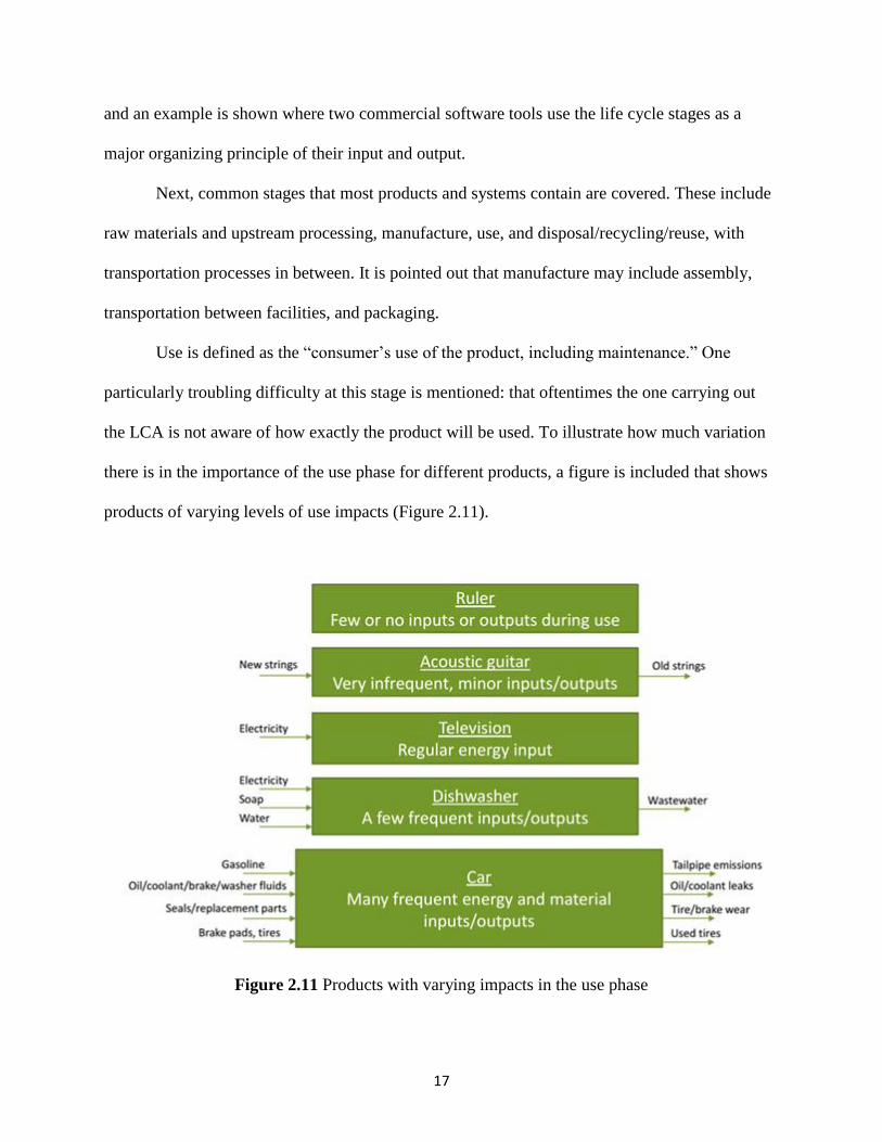
Use is defined as the “consumer’s use of the product, including maintenance.” One
particularly troubling difficulty at this stage is mentioned: that oftentimes the one carrying out
the LCA is not aware of how exactly the product will be used. To illustrate how much variation
there is in the importance of the use phase for different products, a figure is included that shows
products of varying levels of use impacts (Figure 2.11).
Figure 2.11 Products with varying impacts in the use phase

18
Disposal/recycling/reuse is defined as “getting rid of the product at the end of its life.” A
parallel to the use phase is drawn here, in that, again, there might be uncertainty about how a
given product is disposed of if the product is used by the public. In addition, recycling and reuse
can sometimes produce environmental impacts with negative magnitudes, meaning they provide
environmental benefits. An illustration of the disposal stage of a water bottle is shown as an
example of a product that may have different possible types of disposal. The illustration in
Figure 2.12 shows how the various end-of-life options can reenter a product’s life cycle in
different places (or not at all).
Figure 2.12 End-of-life scenarios for a plastic water bottle
Finally, the transportation stage of a product is covered. Transportation often occurs
between various other stages and usually happens multiple times throughout a product’s life
cycle. The transportation stage can be treated separately in the life cycle or simply grouped with
other life cycle stages. Some common modes of transportation are pointed out to demonstrate the
range of options including rail, containership, pipeline, cargo plane, truck, and multimodal
means.

19
2.6 Module α4: LCIA Optional Elements: Grouping, Weighting, and Normalization
This module begins by reinforcing the four phases of an LCA (Figure 2.2) to remind listeners
where the LCIA phase is within the LCA process. The module visits the four optional elements,
which include grouping, weighting, normalization, and additional data quality analysis.
Additional data quality analysis is not covered further in the module, but the other items are.
Grouping is discussed first, and examples of four possible grouping schemes for environmental
impact categories are presented as in Figure 2.13.
Figure 2.13 Examples of grouping schemes for LCA impact categories
An example of grouping by impact medium (air, water, soil, and resources) is given in
graphical format along with results from an LCA on lighting products by Scholand and Dillon
(2012). Next, an example of grouping by priority is shown, where the authors of the module
series group impact categories by high, medium, and low priority using data from Lippiatt
(2007).

20
Normalization is introduced as presenting “impacts as a relative magnitude to a reference
value.” Normalization is useful as both an interpretation aid and as an error-checking method,
but sometimes it results in unintended consequences. Internal normalization and external
normalization are differentiated: internal is normalizing by an alternative in the study, and
external is normalizing by an outside reference. A theoretical example is shown to demonstrate
this difference with a city transit bus and a school bus, normalized internally and then externally
to a United States daily per capita reference. Further examination of the pros and cons of each
normalization style is covered, and the suggestion to potentially use both styles is made. In the
next few slides, some sets of actual LCA data are shown, where the results are normalized
internally (Ally and Pryor 2007, Cooney 2005) and externally (Langfitt and Haselbach 2014) to
demonstrate how the type of normalization can affect results appearance and how even different
types of internal normalization are possible (at least by a baseline, by maximum, and by sum).
An example of this is shown in Figure 2.14. Source details for what the authors think is a fairly
comprehensive list of external normalization databases for the United States are presented (Bare
et al. 2006, Lautier et al. 2010, Laurent et al. 2011, Kim et al 2013, Ryberg et al. 2014).
Figure 2.14 Comparison of internally and externally normalized results (data from Scholand and
Dillon 2012)

21
The last topic in the module, weighting, is discussed. Weighting means applying a
valuation scheme to the impact categories such that categories more important to the decision-
maker receive more attention. There are various weighting schemes published in the literature,
and these are sometimes used to aggregate overall product scores. However, it is pointed out that
weighting adds subjectivity to LCA results, that characterized results must also be presented with
weighted results, and that weighting is not allowed in comparative studies. Three types of
weighting scheme development procedures are then outlined, including the panel method,
monetary valuation methods (see Ahlroth et al. 2011), and distance-to-target method. The
numerical values of four published weighting schemes from the literature are presented (Lippiat
2007, PE International 2012). Finally, a software tool that uses weighting in its output is shown:
Building for Economic and Environmental Sustainability (BEES).
2.7 Module α5: Data Types and Sources
Module α5 begins with a discussion on the importance of data in LCA. Because LCA is
essentially an accounting method, poor or missing data can significantly affect results through
bias or uncertainty, and no single database exists; thus, data for various studies are sourced and
collected from disparate locations. It is emphasized that processes contributing more to the
overall impact of a product are more important from a data- quality perspective, and this idea is
presented in Figure 2.15 (reprinted with permission from Simonen 2014).

22
Figure 2.15 Priority for increasing data quality of processes in an LCA (Simonen 2014)
Data types are covered next, which include primary data (directly measured by the
researchers) and secondary data (obtained from databases, literature, etc.). Proxy data are defined
as “data for a product or process that is assumed to be roughly equivalent to the product or
process of interest.” The remainder of the module focuses on data sources, and this is first
introduced by defining, at a high level, where data could come from and categorizing them as
primary, secondary, and estimated, as shown in Figure 2.16.

23
Figure 2.16 Overall categories of data sources
Some journals that commonly include LCA case studies that could be targeted for
secondary data collection are listed. Life cycle inventory databases are introduced next. These
databases are typically the easiest way to obtain large amounts of LCA data, can be integrated
into software programs, usually contain extensive documentation (metadata), and come in both
free and paid formats depending on the source. Some common LCI databases are presented, with
a focus on those including United States data. One to two slides are dedicated to each of these
databases and typically include information on who produced the data set, how many
products/processes are included and whether they are paid or free, what industry the
products/processes are focused on (if applicable), and how the dataset can be obtained. Finally,
the last instructional slide of the module contains database information for other countries
(Europe excluded). At the time of initial publication, this information includes only China and
India, but the intention is to add to this list as countries develop databases and the module
authors become aware of those developments.

24
2.8 Module α6: Environmental Product Declarations
Environmental product declarations (EPDs) are first defined using a definition from EPD
International (2015), which states that an EPD is “a verified document that reports environmental
data of products based on life cycle assessment (LCA) and other relevant information and in
accordance with the international standard ISO 14025 (Type III Environmental Declarations).”
The EPD is framed in the greater context of LCA, by explaining that LCA is a method and EPD
is a report (which typically uses the LCA method as an input) (Simonen and Haselbach 2012).
Environmental product declarations are placed within the ISO standards on eco-labeling as a
Type III label governed by ISO 14025. Each of these three types of labels is discussed using
Figure 2.17 as a guide.
Figure 2.17 ISO eco-labeling scheme
The overall objective of an EPD is to “drive the production and use of environmentally
sustainable products.” Four specific sub-objectives are defined as providing accurate
environmental information, giving purchasers the power to consider environmental information

25
in decisions on which products to purchase, encouraging the use of more environmentally
friendly products, and making data collection easier for large systems.
The required content of an EPD according to ISO 14025 is presented (ISO 2006c),
including information on the company producing the product, a description of the product, a
reference to the product category rule (PCR) used to develop the EPD, information on LCA
modeling choices, data sources used, LCI results, LCIA results, interpretation, etc. Optional
content for EPDs, such as social impacts and the recycled content used, is also covered.
At this point, it becomes necessary to introduce PCRs, which are defined as “‘rules’ on
what to include and how to compute inputs and outputs to enable ‘apples-to-apples’ comparisons
between products and enable the creation of EPDs’” (Simonen and Haselbach 2012). Further
description and a sample listing of some existing PCRs are provided. The required content of a
PCR is then presented and modules (from this module series) discussing concepts pertinent to
those requirements are cross-referenced. Which of these requirements need to be “identical” and
which need to be “equivalent” under ISO 14025 (ISO 2006c) are identified. The fact that
multiple groups are responsible for creating PCRs results in large inconsistencies between sets of
rules created for very similar product categories. A table from Subramanian et al. (2011) is
reprinted to demonstrate inconsistencies actually found when comparing various PCRs.
A sample listing of program operators (companies and organizations that produce PCRs)
is presented, with a separate United States-focused list and international list. As a transportation
example, the table of contents for an existing PCR for highways is reprinted, and content from
the PCR is summarized (International EPD System 2014).
Switching back to EPDs, a diagram representing the overall process for developing an
EPD is presented (Figure 2.18). Environmental product declarations are usually designed for

26
institutional buyers rather than for average consumers (Stevenson and Ingwersen 2012), so most
EPDs are marketed toward businesses and companies, though sometimes they are used as parts
of regulations.
Figure 2.18 EPD development process
A list of sources for finding many EPDs is presented, and it is noted that for an EPD, the
“concept is simple...implementation is not.”

27
CHAPTER 3.0 GROUPS B AND β: ENVIRONMENTAL IMPACT CATEGORIES
The modules in the B and β groups cover each of the most common environmental impact
categories in LCA. In this module series, the focus is put on emissions-based impact categories,
though some effort is dedicated to resource and other impact categories. This is roughly in line
with the prevalence of these impact categories in the LCA study literature.
3.1 Module B1: Introduction to Impact Categories
Module B1 begins by introducing what an environmental impact category is through the ISO
definition of a “class representing environmental issues of concern to which life cycle inventory
analysis results may be assigned” (ISO 2006a). The three overall classes of impact categories are
presented: human health, ecosystems, and resources. Next, the most common emissions-based
impact categories are listed, along with alternative names for those same impacts, and with
reference to the B module that covers each. These include the following:
Acidification Potential (AP)
Ecotoxicity Potential (ETP)
Eutrophication Potential (EP) (Also: Nutrification)
Global Warming Potential (GWP) (Also: Climate Change)
Human Toxicity Cancer Potential (HTCP) (Also: Human Health Cancer)
Human Toxicity Non-Cancer Potential (HTNCP) (Also: Human Health Non-Cancer)
Human Health Criteria Air Potential (HHCAP) (Also: Human Health Particulates)
Stratospheric Ozone Depletion Potential (OPD) (Also: Ozone Layer Depletion)
Smog Creation Potential (SCP) (Also: Photochemical Ozone Creation)

28
Other impact categories that are not emissions-based are briefly covered. These include
various types of resource depletion, energy use, land use, water use, landfill use, nuisance (odor,
sound), indoor air quality, and radiation.
The process for computing environmental impacts (the LCIA phase) is reintroduced
using Figure 2.4. The relationship between inventory flows (i.e., masses of emissions) and
environmental impacts is further examined using global warming and acidification potentials as
examples. Figure 3.1 is used to represent that while CO2 and CH4 both contribute to global
warming potential, 1 kg of CO2 has less of an effect than 1 kg of CH4.
Figure 3.1 Exploration of potency of various global warming potential substances
Since life cycle assessment is designed to assess the impacts of humans on the
environment, only anthropogenic (human caused) emissions are considered. However, some
natural sources of emissions contribute to these impact categories, such as volcanoes emitting
SO2, respiration of humans emitting CO2, and forests emitting volatile organic compounds
(VOCs). Each type of environmental impact could be considered to have different breadths of
geographic coverage. That is, some types of impact have local, regional, and global, or multiple
scales depending on the transport, deposition, and lifetimes of the emitted substances.
The terminology impact category indicator is then introduced by its ISO 14040 definition
of a “quantifiable representation of an impact category” (ISO 2006a). Examples are shown using

29
four impact categories and samples of indicators that could be used in those categories (Figure
3.2). Impact category indicators come in two basic types: midpoint (direct effects) and endpoint
(final effects). A flowchart shows the process from emissions to final impacts for ozone
depletion, with midpoint highlighted in this flow diagram as a process called “ozone depleted
based on substance’s reactivity/lifetime” and endpoint as “effects on human health, plants,
organisms, buildings, etc.” (Bare et al. 2002).
Figure 3.2 Impact category indicator examples
Finally, the concept that all impacts in LCA are “potential” is explained. This means that
impacts may or may not happen in the magnitudes predicted depending on mechanism modeling,
spatial and temporal considerations, data quality, assumptions, etc.
3.2 Module B2: Common Air Emissions Impact Categories
This module begins by introducing the main points from Module B1, including that impacts are
“potential,” that only anthropogenic emissions are included, that different substances contribute
different amounts to each impact category, and that impact categories have different geographic

30
scales of impact. A listing of emissions-based impact categories covered in the module series is
reintroduced, as well as a list of categories that are not covered in detail.
The remainder of the module uses two slides per each of the four impact categories
specifically addressed in this module (acidification potential, global warming potential, smog
creation potential, and stratospheric ozone depletion potential). The first slide is an introduction
to the category, including a brief description, the geographic scale of impact, units commonly
used as indicators, a figure representing the category, etc. The second slide for each impact
category presents the major sources (i.e., industries/sectors), major substances that contribute to
the impact category in the United States (based on Ryberg et al. 2014), a one-sentence statement
of the category midpoint, and a listing of possible category endpoints.
Acidification potential is defined as “emissions which increase the acidity (lower pH) of
water and soils.” Common deposition routes are stated, the scale of impacts is reported as local
and regional, the importance of regional variation is emphasized, and the common units used are
identified as kg SO2-eq and mol H+-eq. The major sources are fuel combustion for electricity and
transportation, and agriculture. The major substances are nitrogen oxides, sulfur oxides, and
ammonia. The midpoint is defined as “increased soil and water acidity,” and the endpoint is
identified as damage to organisms, plants, and buildings.
Global warming potential is described as the “increase in greenhouse gas concentrations,
resulting in potential increases in the global average surface temperature.” It is pointed out that
temperature increases happen as a result of the greenhouse effect, that biogenic sources of CO2
are often not included, that this impact category is usually based on a 100-year time scale, that
the geographic scale of impacts is global, and that in nearly every study the indicator used is kg
CO2-eq. Major sources of global warming potential are fuel combustion, agriculture, and
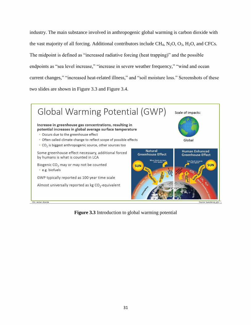
31
industry. The main substance involved in anthropogenic global warming is carbon dioxide with
the vast majority of all forcing. Additional contributors include CH4, N2O, O3, H2O, and CFCs.
The midpoint is defined as “increased radiative forcing (heat trapping)” and the possible
endpoints as “sea level increase,” “increase in severe weather frequency,” “wind and ocean
current changes,” “increased heat-related illness,” and “soil moisture loss.” Screenshots of these
two slides are shown in Figure 3.3 and Figure 3.4.
Figure 3.3 Introduction to global warming potential

32
Figure 3.4 Global warming potential sources, substances, midpoint, and endpoint summary
The next two categories covered are ozone depletion and smog creation. Because both
categories are based on change in ozone concentration, this gas is introduced. It is explained that
ozone near earth’s surface (in the troposphere) is considered “bad ozone,” and ozone high in the
atmosphere (in the stratosphere) is considered “good ozone.” Ozone depletion is discussed first
and defined as “reduction of ozone concentration in the stratosphere.” Ozone depletion is
primarily caused by chlorofluorocarbons (CFCs) and halons, has become much less of an issue
since the enactment of the Montreal Protocol in 1987, is almost universally expressed as kg
CFC-11-eq, and has a global scale of impacts. The major sources are manufacturing, fire
extinguishers, and refrigeration systems. The midpoint is “decrease in stratospheric ozone
concentration,” and potential endpoints include “skin cancer,” and “crop, materials, and marine
life damage.”
Finally, smog creation potential, defined as “increased formation of ground level ozone,”
is reviewed. Smog creation potential is formed by reactions of NOx, VOCs, and other pollutants

33
in the presence of sunlight. The effects of various substances that contribute to smog formation
vary based on air composition, sunlight, weather, geography, and exposed population. The scale
of impacts is local, and the three units typically used are kg O3-eq, kg C2H4-eq, and kg NOx-eq.
Major sources include cars and other vehicles, industrial processes, and energy production. The
midpoint is “increase in ground-level ozone concentration,” and the possible endpoints are
“reduced lung function,” “aggravated asthma,” “vegetation damage,” and “eye irritation.”
3.3 Module B3: Other Common Emissions Impact Categories
This module begins with the same introduction as Module B2 and uses the same two-slide
format per impact category. It covers in detail eutrophication, human toxicity, ecotoxicity, and
human health particulate potentials.
Eutrophication potential is defined as “excessive biological activity of organisms due to
over-nutrification.” Eutrophication can lead to oxygen deficiency and the death of aquatic
organisms, especially following algal blooms. The scale of impacts is local, and the four
common units used to express the category results are kg PO43—
eq, kg P-eq, kg NO3-eq, and kg
N-eq. Major sources are agricultural runoff, storms and wastewater, septic field seepage, and
fossil fuel combustion. The midpoint is defined as “excessive biological growth, especially of
algae,” and possible endpoints are defined as “death of aquatic life,” “loss of biodiversity,” and
“foul odor.”
Human toxicity potential is defined as “effects to individual human health that can lead to
disease or death.” Human toxicity is often differentiated by cancer and non-cancer effects,
includes both causing and aggravating conditions, is particularly uncertain in its characterization
of impacts, and is often characterized based on a system called USEtox. The scale of impacts
could be local, regional, or global, and common units used to express impacts are kg benzene-eq,

34
kg toluene-eq, and cases (equivalent to comparative toxic unit, CTU). Major sources of impacts
are mining, agriculture, manufacturing, and energy production. Main substances include dioxins,
chromium, arsenic, zinc, benzo(a)pyrene, and formaldehyde. The midpoint is defined as “general
health effects on humans,” and possible endpoints include asthma, cancer, heart disease, etc.
Ecotoxicity potential is defined as “impacts on whole ecosystems that can decrease
production and/or biodiversity.” This category is more focused on whole system impacts than on
individual impacts (unlike human toxicity), characterization is usually based on the USEtox
system (like human toxicity), and there is a great deal of uncertainty in much of the
characterization of substances in this impact category. The scale of impacts is local to regional,
and the units commonly used to express this category are kg 2,4-dichlorophenoxy-acetic acid and
“potentially affected fraction.” Major sources of ecotoxicity are mining, agriculture,
manufacturing, and energy production. Main substances include zinc, copper, and organic
chemicals. The midpoint is defined as “general degradation of ecosystems (no true midpoint),”
and possible endpoints include “decreased population” and “decreased biodiversity.”
Finally, the human health particulates impact category concerns “health issues related to
increased respiration of very small particles.” These particulates are both directly released from
systems and form in secondary reactions; they can cause cancer and cause or aggravate
respiratory disease, and they are usually more severe for certain high-risk individuals. The scale
of impacts is local, regional, and global, and the units generally used to express the category are
kg PM2.5-eq, kg PM10-eq, and disability adjusted life years (DALYs). Major sources of the
substances that cause particulate health impacts are fossil fuel combustion, wood burning, and
dust from roads and fields. The main substances include directly emitted particulate matter, SOx,
and NOx. The midpoint is defined as “increased human exposure to particulate matter,” and the

35
possible endpoints as “heart health effects,” “aggravated asthma,” “decreased lung function,” and
cancer.
3.4 Module β1: Global Warming Potential
Global warming potential (GWP) is defined, its relationship to the term climate change is
indicated, the greenhouse effect is identified as the underlying mechanism, and common
greenhouse gases (GHG) are identified. The greenhouse effect is then described in common
terms (acting “like a blanket”) and in technical terms (radiative forcing due to short- and long-
wave radiation differences). It is noted that the greenhouse effect is necessary for life on Earth,
but additional GWP from human activity is the basis of the impact category.
Possible endpoint effects are identified (U.S. EPA 2015a). A few of these effects include
stronger storms, rising sea level, and less ice, but the magnitudes of these endpoint effects are
uncertain. Quantitative observations of possible effects of global warming that have already been
observed are presented, including changes in temperature, sea ice extent, sea level, and
precipitation. The characterization equation is GWP= Σi (mi x GWPi) where, GWP=global
warming potential in kg CO2-eq of full inventory of GHG, mi = mass (in kg) of inventory flow
‘i’, and GWPi = kg of carbon dioxide with the same heat trapping potential as 1 kg of inventory
flow ‘i’.
The GWP characterization factors for various common substances are shown for 100-
year GWP in the TRACI 2.1 impact methodology (Bare et al. 2012). Major sources of each
substance and the approximate amounts emitted in the United States in 2013 are presented (U.S.
EPA 2015b). Major sources (fossil fuel combustion, manufacture of cement, land use change,
etc.) and sinks (ocean dissolution, photosynthesis, limestone, etc.) of GHG are identified.

36
The timescale of analysis is highly influential with GWP due to different residence times
of GHG in the atmosphere. This influence is demonstrated with a graph, showing the fraction of
various GHG remaining after time of release. More detail is provided on the residence time of
CO2, demonstrating the variation in estimates (Jacobson 2005, Hewitt and Jackson 2009, Stumm
and Morgan 1996, Archer and Brovkin 2008), and a figure is included that shows the sinks of
CO2 over time. Biogenic CO2 is defined as CO2 “released from recently living material.” Wood,
ethanol, and wastewater are given as examples. While it is common to assume that this release is
carbon neutral, reasons why this assumption may be poor in many cases is explained. Figure 3.5
is an example of 100-year GWP, also done for 20-year GWP.
Figure 3.5 Global warming potential example calculation
The results are later used to demonstrate how using different timescales can influence
results. The question of what time frame to use is posed and briefly explored.

37
3.5 Module β2: Acidification Potential
Acidification potential is defined, the major substances are outlined, the scale of impacts is stated
to be local and regional, and deposition routes (wet, dry, and cloud) are listed. These deposition
routes are illustrated in a graphic. Acidification is defined with respect to the pH scale (i.e., lower
pH=greater acidity), typical units used to express acidification are listed, and the potential
endpoint effects on animals, plants, and materials are listed. Here it is pointed out that different
aquatic species have different tolerances for acidity increase, demonstrated in a figure from the
U.S. EPA (2006b) and reprinted here as Figure 3.6.
Figure 3.6 pH change tolerance of various aquatic species (U.S. EPA 2006b)
The equation for acidification potential is given as the sum of each emission times its
acidification potential characterization factor. A listing of characterization factors for
acidification potential for a number of common substances from TRACI 2.1 is given (Table 3.1).
These factors are usually based on stoichiometry of moles H+ released.

38
Table 3.1 Acidification potentials of selected substances in the TRACI 2.1 methodology
Since sulfur oxides (SOx) and nitrogen oxides (NOx) are two of the largest contributors to
acidification and both come significantly from the transportation sector, inclusive species and
sources are identified. Sulfur oxides can form sulfurous acid when dissolved in water. Major
sources of SOx include power plants, industrial facilities, mobile sources, and industrial
processes. Nitrogen oxides can form nitric acid when dissolved in water. A major source of NOx
is fuel combustion.
The importance of regional variation is discussed, including differences in flora and
fauna, current pH balance, buffering capacity, and pollutant transport properties between regions.
One effort to account for this regional variation, regional characterization factors in the TRACI
impact methodology (Bare et al. 2002), is covered. An important point is made that this impact
category does not include acidification of oceans by CO2 dissolution. Finally, this module ends
with the same summary slide as that used for acidification potential in Module B1.
3.6 Module β3: Ozone Depletion Potential
This module begins by revisiting what ozone is. It is explained that while two impact categories
in LCA are concerned primarily with ozone, one is concerned with depletion and the other is
concerned with formation. The reason for this difference is that in the stratosphere, ozone creates
a natural protective layer from UV radiation, but in the troposphere, it can be breathed in and

39
negatively impact human health. A profile of ozone concentration from surface level to 35 km is
shown to demonstrate where local peaks are in ozone (i.e., in the ozone layer and near Earth’s
surface).
Ozone depletion potential (ODP) is specifically covered, noting the scale of impacts as
global, and identifying additional UV radiation from ozone depletion as having effects on
humans, crops, and the built environment. Ozone depletion potential covers both a general
decrease in concentration and more severe decreases in localized holes, and ODP is not a major
contributor to global warming. Next, the midpoint (“ozone depleted based on substance’s
reactivity/lifetime”) and endpoints (effects of increased UV) are identified using a diagram
depicting emissions to effects.
Major classes of substances are reviewed, including their abbreviation, name, general
severity (in causing ozone depletion), main uses, and specific examples. These classes include
halons, CFCs and HCFCs (Table 3.2.) Nitrous oxide may be a potential major contributor to
ozone depletion, also, due to reductions in traditional ozone depleting substances (Ravishankara
et al. 2009).
Table 3.2 Classes of ozone depleting substances (selection)

40
Ozone depletion potential chemistry is discussed at the overview level, including natural
equilibrium reactions (Figure 3.7) and chlorine/bromine catalyzed reactions (due to the presence
of ODP substances).
Figure 3.7 Natural equilibrium reactions involving stratospheric ozone
The equation for characterizing ozone depletion is shown alongside a table of
characterization factors from TRACI 2.1 for a selection of substances. Ozone holes are discussed
including that they usually form at the Arctic and Antarctic, with the latter location having the
larger hole, and that they mostly form due to polar stratospheric clouds (World Meteorological
Organization 2006). The Montreal Protocol is reviewed including that the international treaty
was agreed upon in 1987, universally ratified by the members of the United Nations, calls for
phase-outs and eventual replacement of ODP substances, and has been largely successful in
reducing ozone depletion (Fahey and Hegglin 2010). As a result, the U.S. Environmental
Protection Agency (U.S. EPA 2010) has predicted that the ozone hole will fully recover in about
50 years.

41
3.7 Module β4: Smog Creation Potential
Module β4 begins with the same overview of ozone as in Module β3. Ozone is formed mostly by
reactions of NOx and VOCs in the presence of sunlight, its effects vary based on regional factors,
and the geographic scale of impacts is local. The common units are given.
The term smog is a portmanteau of smoke and fog, but modern smog is actually mostly
ground-level ozone with other constituents including peroxyacetyl nitrates, aldehydes, and
remaining NOx and VOCs which have not converted to ozone (Klöpffer and Grahl 2014). Smog
can have negative impacts on human health (mostly respiratory-related), vegetation, and quality
of life (e.g., decreased visibility). Most effects are short-term, but some can be chronic.
Smog forms through reactions of NOx and VOCs/CO in the presence of solar radiation.
Vehicle emissions are major anthropogenic sources of these compounds; forests are a major
natural source of VOCs. A simplified chemistry of smog formation is presented, including both
the standard NOx cycle (does not create net ozone) and the NOx cycle augmented by VOCs (does
contribute net ozone) (see Figure 3.8).
Figure 3.8 Simplified chemistry of smog formation with CO used in the HOx cycle

42
The equation for characterizing smog creation potential is then given along with a sample
listing of some substances’ characterization factors in TRACI 2.1, and regional variation in
effects is covered in detail. Landscape features (like canyons) can trap pollutants, leading to
increased smog formation, and areas with more sun tend to have greater potential for ozone
formation. Pictures of Los Angeles and Mexico City under the cover of smog are shown. Pre-
existing NOx and VOC concentrations can significantly impact the effect of further emissions of
these gases on smog formation, with an ozone isopleth used to demonstrate this point. Usually,
these types of local variations are not accounted for in LCA, but a few attempts to use regional
characterization factors and more detailed models are identified (Bare et al. 2002, Alcamo et al.
1990, Shah and Ries 2009). The final slide is a summary of major sources, main substances, the
midpoint definition, and possible endpoints.
3.8 Module β5: Eutrophication Potential
This module begins with an introductory slide that defines eutrophication potential (EP) and its
largest forcers (nitrogen and phosphorus), and explains that these nutrients are needed to support
growth, but over-nutrification is a concern, and that local variation can be important. Nitrogen
and phosphorus compounds are the main substances of interest; these come mostly from
agriculture, storm water, wastewater, fossil fuel combustion, and household activities.
The equation for characterizing eutrophication potential along with a sample listing of
characterization factors for various substances in the TRACI 2.1 methodology are shown next.
Biochemical oxygen demand (BOD) and chemical oxygen demand (COD) are included (Figure
3.9) because they lead to the same endpoint effect (i.e., oxygen depletion) as EP.

43
Figure 3.9 Definitions of BOD and COD (*U.S. EPA 2012, **Eaton et al. 1995)
The concept of a limiting compound or element is covered. In a system with high levels
of nitrogen (compared with phosphorus), adding nitrogen would do little to increase biomass
growth; adding phosphorus would do more, and vice versa. Freshwater is typically phosphorus-
limited, and soil and saltwater systems are typically nitrogen-limited; however, depending on the
characterization model used, this may or may not be accounted for in LCA. These points and the
midpoint units typically used in each setting are shown in the module (see Figure 3.10).
Figure 3.10 Typical limiting nutrients in freshwater, soil, and saltwater environments

44
Deposition and transport, such as directly running off into soil or water or being emitted
to air then subsequently deposited, are important. Emitting a substance does not mean that it will
reach water or soil, and substances emitted in one location can travel far to reach another.
Endpoint effects of eutrophication potential are covered including “loss of biodiversity,”
“fish kills,” “shellfish poisoning,” “loss in tourism,” and direct toxic effects to humans in contact
with algae or drinking nitrates. Regional variation is discussed. If eutrophication is near the
“critical load,” adding nutrients may have a greater effect, and some impact methodologies have
attempted to consider this with regional characterization. A figure showing exceedance of
nutrient loading across Europe shows variation from the European Environment Agency (2013).
Finally, the major sources, main substances, midpoint definition, and possible endpoints are
given.
3.9 Module β6: Human Toxicity and Ecotoxicity Potentials
This module includes both human toxicity and ecotoxicity, because the way in which they are
characterized is similar. The first slide is an introduction to human toxicity potential, defined as
“effects to individual human health that can lead to disease and death.” This category is often
split between cancer and non-cancer, only considers direct toxic effects on human health (not
indirect ones like human health effects of climate change), is concerned with large-scale impacts,
and can have impacts on a local, regional, or global scale. Ecotoxicity potential is introduced,
describing it as more focused on whole ecosystem impacts (rather than the health of individuals),
as sometimes split between water and soil, and as having only a local scale of impact.
Differences between human and ecotoxicity are the scale of impact and focus on individuals
versus whole ecosystems. Similarities are that both are concerned with toxic effects.
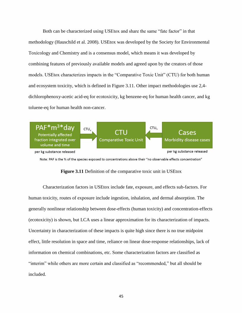
45
Both can be characterized using USEtox and share the same “fate factor” in that
methodology (Hauschild et al. 2008). USEtox was developed by the Society for Environmental
Toxicology and Chemistry and is a consensus model, which means it was developed by
combining features of previously available models and agreed upon by the creators of those
models. USEtox characterizes impacts in the “Comparative Toxic Unit” (CTU) for both human
and ecosystem toxicity, which is defined in Figure 3.11. Other impact methodologies use 2,4-
dichlorophenoxy-acetic acid-eq for ecotoxicity, kg benzene-eq for human health cancer, and kg
toluene-eq for human health non-cancer.
Figure 3.11 Definition of the comparative toxic unit in USEtox
Characterization factors in USEtox include fate, exposure, and effects sub-factors. For
human toxicity, routes of exposure include ingestion, inhalation, and dermal absorption. The
generally nonlinear relationship between dose-effects (human toxicity) and concentration-effects
(ecotoxicity) is shown, but LCA uses a linear approximation for its characterization of impacts.
Uncertainty in characterization of these impacts is quite high since there is no true midpoint
effect, little resolution in space and time, reliance on linear dose-response relationships, lack of
information on chemical combinations, etc. Some characterization factors are classified as
“interim” while others are more certain and classified as “recommended,” but all should be
included.

46
Sources include agriculture, mining, manufacturing, storm water, fuel combustion, and
waste combustion, as summarized in Figure 3.12. The equation for characterization and a
sampling of characterization factors for various substances for ecotoxicity, human health cancer,
and human health non-cancer, are provided separately. Summary slides cover major sources and
substances, midpoints, and possible endpoints for ecotoxicity and human health potential.
Figure 3.12 Sources of chemicals that cause human and ecological toxicity
3.10 Module β7: Human Health Particulate Matter Potential
Human health particulate matter potential is defined as “health issues related to increased
respiration of very small particles” and is sometimes called “criteria air pollutant potential.” The
scale of impacts is local, regional, and global. The particulates are both solids and liquid
droplets, and classifications based on hydraulic diameter are presented (coarse PM, PM10, PM2.5,
and ultrafine PM). Particulate matter is formed through primary and secondary pathways (Figure
3.13.) Primary means that the particulates are directly released such as in materials handling,
windblown dust, and combustion. Secondary particulate matter is that formed from reactions of

47
non-particulate emissions, such as SO2, NO2, NH4, and VOCs, and depends on atmospheric
conditions. Some are more likely to form in summer, while others are more likely to form in
winter.
Figure 3.13 Particulate matter formation pathways
Sources of particulate matter are discussed using a pie chart from the U.S. EPA (2005).
Both anthropogenic and natural sources are identified. Variation in the composition of particulate
matter by region reveals how various sources from different regions affect PM composition (e.g.,
high proportion of sulfates where coal-fired power plants are common).
Transport is important. Larger particulate matter cannot travel far due to settling out fast,
while the smaller particulate matter can stay airborne much longer, as shown in Figure 3.14.
Cities in the western United States tend to have a larger share of particulate matter from local
sources, whereas the opposite is so in the eastern United States.

48
Figure 3.14 Illustration of the approximate maximum range of PM10 (top) and PM2.5 (bottom)
Human health effects from particulate matter are mostly related to heart and lung
function and cancer, and various specific effects are identified in the module. Pope III et al.
(2002) identifies the increased risk of all-cause, cardiopulmonary, and lung cancer mortality due
to increases in PM2.5 concentration. Non-human health effects (on plants and visibility) are
briefly identified.
Concentrations of PM2.5 around the world and around the United States are presented in
satellite-derived, time-averaged maps (NASA 2010). The equation for characterization is
presented as well as a table of characterization factors in the TRACI 2.1 methodology, which
reveals that under that methodology PM2.5 is about 4–5 times as severe as PM10. Finally, major
sources and substances, the midpoint definition, and possible endpoints are summarized.

49
3.11 Module β9: Impact Assessment Methodologies
The life cycle impact assessment (LCIA) phase of LCA is revisited showing the various
mandatory steps. One of those steps is “characterization model selection,” and that is the focus of
this module. Characterization models come in many different types, have different geographic
relevance, have different time coverage, and may include different optional elements. A sample
procedure for calculating impacts in the LCIA phase is presented, with identification of how the
chosen impact assessment methodology could affect each step. The three schools of thought for
developing impact methodologies (distance-to-target, midpoint, and damage) are identified as
well as the average update frequency, recommendations for relevance based on age, and
criticism surrounding impact methodologies in general. A compiled listing is shown of most of
the impact assessment methodologies in existence, along with the school of thought used to
develop them and whether they are covered in the module (see Figure 3.15).
Figure 3.15 Summary of impact assessment methodologies and their schools of thought
The remainder of the module is dedicated to a discussion of impact methodologies listed
under “covered in this module” in Figure 3.15 with two slides each. The first slide is a summary
that usually identifies the full name (most of the names are acronyms), the creator, the date of

50
last update, geographic area of coverage, school of thought, a link to the methodology’s website,
and any optional data provided by the methodology (e.g., normalization references). The second
slide of each impact methodology lists the impact categories covered, and in many cases includes
a flow diagram to show how impacts are converted from inventories to final results.

51
CHAPTER 4.0 GROUPS G AND γ: GENERAL LCA TOOLS
Software can often be useful in carrying out an LCA. However, there are many different reasons
why software might be useful and many different options for software tools. The modules in
these groups cover software tools at both an overview level and a tutorial level (the latter only
for a smaller subset).
4.1 Module G1: General Paid LCA Software Tools
Reasons why software is frequently used in carrying out LCA include reduction in time and
effort, decreased errors, increased modeling capabilities, data organization, and automatic
creation of figures and tables. The cost, learning curve, and complexity of the tools vary. An LCI
for crude oil illustrates the data complexity involved (NREL 2015). Some common LCA-paid
software tools are listed including GaBi, SimaPro, Quantis Suite, and Umberto. Each software
tool is summarized in three slides.
GaBi integrates its own databases into the tool, though other databases can be integrated.
Users input processes and flows in graphical format, and GaBi calculates LCA results using
sequential modeling. The software operates on a one-license-per-computer principle. Output
defaults to bar graphs, showing impact-category indicator results split by process (Figure 4.1).
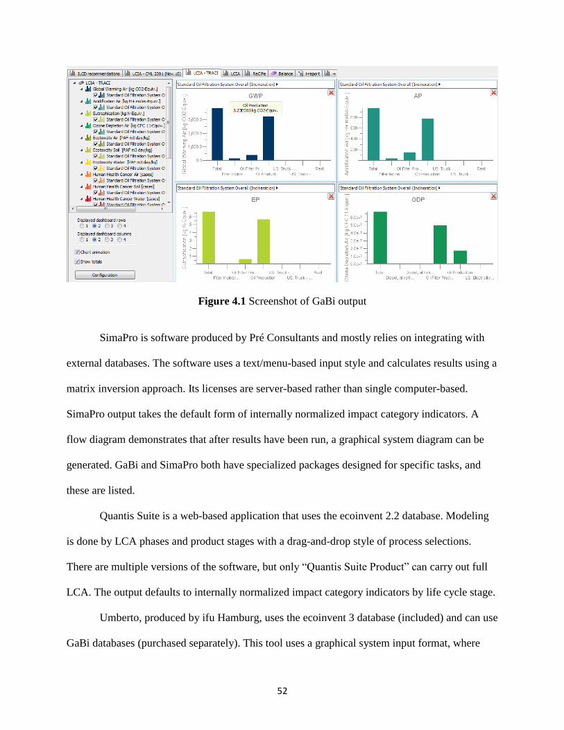
52
Figure 4.1 Screenshot of GaBi output
SimaPro is software produced by Pré Consultants and mostly relies on integrating with
external databases. The software uses a text/menu-based input style and calculates results using a
matrix inversion approach. Its licenses are server-based rather than single computer-based.
SimaPro output takes the default form of internally normalized impact category indicators. A
flow diagram demonstrates that after results have been run, a graphical system diagram can be
generated. GaBi and SimaPro both have specialized packages designed for specific tasks, and
these are listed.
Quantis Suite is a web-based application that uses the ecoinvent 2.2 database. Modeling
is done by LCA phases and product stages with a drag-and-drop style of process selections.
There are multiple versions of the software, but only “Quantis Suite Product” can carry out full
LCA. The output defaults to internally normalized impact category indicators by life cycle stage.
Umberto, produced by ifu Hamburg, uses the ecoinvent 3 database (included) and can use
GaBi databases (purchased separately). This tool uses a graphical system input format, where

53
processes are placed into specific life cycle stages. Umberto has multiple versions of the
software with “NXT LCA” and “NXT Universal” both able to carry out full LCA. The output of
Umberto defaults to showing impact category indicators and a bar diagram from each life cycle
stage.
All of the software tools have similar features, the major differences being mostly related
to the user interface. Links to free trial websites are included.
4.2 Module G2: Free LCA Software Tools (Non-Transportation)
There are many free software tools available for LCA. Some include only an interface (where
data must be input by the user or from a database); others are fully packaged and simplified (data
included and simpler inputs are made). The module summarizes OpenLCA, Building for
Environmental and Economic Sustainability (BEES), Athena Impact Estimator for Buildings,
and Economic Input-Output Life Cycle Assessment (EIO-LCA). Each tool has three slides,
consisting of an introduction, screenshots of input, and screenshots of output.
OpenLCA is produced by GreenDelta as an open-source software and an interface-only
style software. It has modeling capabilities similar to the paid software tools covered in Module
G1. Data must be input by manual entry, by connecting a free database, or by connecting a paid
database. Systems are built using a graphical interface of inserting processes and drawing flows.
Output can be shown in many forms such as graphs by flow contributions, by impact
contributions, and in Sankey diagrams with various impact methodologies.
Athena Impact Estimator allows for modeling of whole buildings based on a large set of
inputs, which include detailed building parameters (such as width, span, and live load of a floor
assembly) and the building location. Output from this tool is in the form of impact category

54
indicators in the TRACI 2.1 impact methodology, with the notable omission of human health
cancer, human health non-cancer, and ecotoxicity categories.
BEES is an online tool produced by the National Institute of Standards and Technology
(NIST) for analyzing environmental and economic aspects of building products. Nearly 200
products are included such as concrete, roofing, insulation, and paving. Input to the tool consists
of choosing an environmental impact category weighting scheme and products by a product
category hierarchy. Transportation distances can also be included. The output of BEES takes the
form of individual graphs for each impact category indicator by life cycle stage or by inventory
flow and a table with the numerical data using the TRACI impact methodology (Figure 4.2).
Figure 4.2 BEES output by life cycle stage and by environmental flow
The EIO-LCA is an online tool produced by Carnegie Mellon University. This tool
calculates environmental impacts using a methodology of relating economic activity to
environmental impacts to exploit preexisting economic models to estimate environmental
impacts of sectors. Therefore, the tool’s input consists of an economic value of product in any of

55
hundreds of sectors for either the United States, Canada, China, Germany, or Spain. The tool
outputs LCA results in the TRACI methodology using a spreadsheet format that shows how
much impact contribution comes from each sector that feeds into the sector of interest as well as
the overall impact in that sector to generate the input dollar value of economic activity in the
sector.
4.3 Module G3: Free LCA Software Tools (Non-Transportation)
Module G3 introduces various topics of interest in transportation LCA and points out that many
studies termed “LCA” in the transportation sector are actually only inventories of GHG and
regulated emissions (Figure 4.3), although some report impact category indicators.
Figure 4.3 Greenhouse gases and regulated emissions
Four free tools for LCA in the transportation sector are introduced: the Greenhouse
Gases, Regulated Emission, and Energy Use in Transportation Model (GREET), the Fuel and
Emissions Calculator (FEC), the Pavement Life-Cycle Assessment Tool for Environmental and
Economic Effects (PaLATE), and Athena Impact Estimator for Highways. A slide of
introductory material introduces each tool, and screenshots of input and output are shown.
Developed by Argonne National Laboratory, GREET performs environmental
assessment of transportation fuels used in passenger vehicles. Over 100 fuel-production
pathways and 50 vehicle types are included. The output is GHG and regulated emissions only,

56
not impact category indicators. The tool can be used to examine the production of materials and
fuels, and the use of fuels in vehicles. Examples are shown for selecting conventional diesel fuel
production (Figure 4.4) and a liquefied natural gas car.
Figure 4.4 Well-to-pump diagram for conventional diesel fuel in GREET
The FEC is produced by Georgia Tech and is spreadsheet-based. It is similar to GREET
in that it outputs GHG and regulated emissions inventories, but FEC is used for buses and rail,
and allows the user to input location and duty cycle. A screenshot of the input for a bus is shown
as well as a graph demonstrating duty cycle. Emissions are broken down into upstream fuel, on-
road, and per route.
PaLATE is produced by UC Berkeley and analyzes the environmental and economic
impacts of pavement. The tool is excel-based and can only be acquired by personal
communication with its creator. PaLATE output includes the inventory results of air emissions
and leachates, as well as GWP and human toxicity potential impact category indicators. The
input includes roadway design parameters, construction materials, maintenance materials, and
construction equipment.
Athena Impact Estimator for Highways is produced by the Athena Sustainable Materials
Institute. It analyzes initial paving materials, highway use, maintenance, and end of life in
Canada. A roadway is built based on roadway geometry, material, and location inputs, with the

57
ability to control factors like construction equipment used. The output can be impact category
indicators in many TRACI 2.1 impact categories (excluding human health cancer, human health
non-cancer, and ecotoxicity) or inventories of emissions and uses of energy and resources. These
outputs can be in graphical or tabular format and are split by life cycle stage.
4.4 Module γ1: EIO-LCA Tutorial and Links to GaBi Tutorial
This module begins by providing links to video tutorials on the GaBi software, since extensive
tutorial material is already available and the video format lends itself well to instruction.
The Economic Input-Output Life Cycle Assessment (EIO-LCA) is then detailed. It
calculates environmental impacts based on economic models, and various countries can be
modeled. The procedure used is explained. The environmental impact of producing a certain
dollar value of goods or services in a given sector is calculated by multiplying the environmental
impacts per dollar in each sector contributing to the sector of interest by the amount of economic
activity generated in each sector. Equations for this process are shown in Figure 4.5.
Figure 4.5 Basis for calculating environmental impacts based on economic activity generated

58
The website to access the tool is eiolca.net and the input process is followed in five steps.
In Step 1, the price model is chosen, which must be selected from a list of discrete combinations
of country, year, and either producer or purchaser pricing. In Step 2, the specific industry and
sector of interest is chosen using either a dropdown menu or a search box. In Step 3, the amount
of economic activity of interest in the sector chosen is input in millions of dollars. In Step 4, the
type of output is selected, which may be economic activity, various environmental flows, or
TRACI impact assessment. Step 5 displays information about the included activities in the sector
chosen and has a “run model” button. The output of the tool is shown for 1 million dollars of
economic activity for “asphalt paving materials and block manufacturing” (Figure 4.6).
Figure 4.6 Output of the EIO-LCA for asphalt paving mixture and block manufacture
Custom models allow the user to create a “sector” as a combination of existing sectors or
to alter the economic ties. A link to a tutorial is
(www.eiolca.net/tutorial/ScreencastTutorial/video3.swf).

59
4.5 Module γ2: Building LCA Software Tutorial (BIRDS, BEES)
This module covers two free tools for LCA of buildings—BIRDS and BEES—both produced by
NIST. BIRDS is used for environmental and economic analysis of new commercial buildings; it
is online-based and has a four-step input process consisting of simplistic selections.
Step 1 of BIRDS is to choose the building type from a list of various types of new
commercial buildings. Selection of the number of floors of interest is also part of this input. Step
2 is to select the location of the building, the energy standard followed, and the study period
(length of time). Completing this step provides both a “baseline” (the expected building) and
“alternatives” (other options considered) so that later comparisons can be made between baseline
and alternative selections. Step 3 is to select the environmental impact category weighting
schemes to be used in the study from a list of provided schemes or to create your own. The
module presents a screenshot of brief descriptions of each impact category from the tool. Step 4
consists of choosing the output format, and in the module, “environmental impact” is chosen for
the chart type. Various different baselines (building location, building energy standard, study
period, and impact category weighting scheme) and indicator units (kg eq substance/ft2, kg eq
substance, and change in either) are chosen as examples of the types of results output that can be
achieved.
Results are in the form of graphs with tables below, and a few examples of the results
output are shown. One such example is global warming potential, compared over different study
periods, using the indicator unit of kg CO2-eq, as shown in Figure 4.7.

60
Figure 4.7 Output of BIRDS, comparing global warming potential by varying study period
The focus of BEES is individual building materials. BEES has three input panes. The first
input pane is for selection of environmental impact category weighting schemes, the second is
for weighting between importance of environmental and economic performance, and the third is
for selection of the product of interest. The options for input in each of these three panes are
discussed individually. The distance that products are transported can be modified, and an option
for viewing life cycle inventory results is shown. The module covers the types of outputs that

61
BEES can provide, focusing on environmental impact category indicators, as shown in Figure
4.8. See Figure 4.2, also, where impacts can be viewed by life cycle stage or by substance.
Figure 4.8 Selection of results output styles in BEES

62
CHAPTER 5.0 GROUPS T AND τ: TRANSPORTATION LCA
The modules in these groups provide information that might be relevant only to those in the
transportation sector, whereas previous modules, with the exception of Module G3, which
summarizes some transportation LCA software tools, can be used for many sectors.
5.1 Module T1: Introduction to Transportation LCA and Literature Review
This module presents overview-level information on a few transportation LCA topics. Some
works in this sector are focused on only energy, GHG, and regulated emissions. Other works
include only a few impact categories, rather than a comprehensive set as required in the ISO
standards. Still, many are full LCAs with a large set of impact category indicators.
Four particular groups of transportation topics are covered in the remainder of the
module: pavement, vehicles, fuel, and other infrastructure. For each group, some pertinent
considerations are presented. For example, pavement considerations include “raw materials,
construction, pavement vehicle interaction, preservation, and removed materials.” A few relevant
software tools are listed. For pavement, these are The Pavement Life-Cycle Assessment Tool for
Environmental and Economic Effects, Athena Impact Estimator for Highways, and ECORCE.
For other infrastructure, no tools are listed, as none was found. Finally, there is a brief listing of
literature for each topic. Within each topic discussed, these studies are further grouped based on
their specific focus, such as shown in Figure 5.1.

63
Figure 5.1 Literature review sample table for pavement life cycle assessment
5.2 Module τ3: GREET Tutorial
GREET is the Greenhouse Gases, Regulated Emissions, and Energy Use in Transportation
Model. The outputs that GREET can provide include emissions (GHG and regulated emissions)
and resource use (various fossil and non-fossil energy sources, uranium ore, farming products,
etc.).
Use of the tool is the focus of the remainder of the module. The first slide discusses the
four panes of the software tool (well-to-pump, well-to-wheel, data editors, and simulation
parameters). The well-to-pump pane allows for analysis of producing materials and fuels that go
into cars. Selection is made from a pre-defined list, and various pathways of production are
available for many of these. An example is shown for producing compressed natural gas.
Expansion of individual processes in the production of that fuel is developed to show how data
and data sources may be viewed and, in some cases, edited. Next, selection of the functional unit
is demonstrated, as shown in Figure 5.2, and the results window is highlighted.

64
Figure 5.2 Selection of the functional unit in the GREET well-to-pump pane
The module covers the well-to-wheel pane, in which the operation of the vehicle is also
of interest. The selections are based on vehicle type, organized by the type of fuel used. An
example of analyzing a conventional gasoline car is shown. Methods for adjusting the model
year of cars, percentage of driving in the urban setting, and emissions factors are shown in case
the user desires to make those changes. Finally, results for an electric car is shown (Figure 5.3) to
demonstrate that, while the vehicle operation column does not have any fuel-related emissions,
the total column does because it includes upstream fuel production.

65
Figure 5.3 Emissions of electric car operation quantified in GREET
5.3 Module τ4: Athena Impact Estimator for Highways Tutorial
Use of the Athena Impact Estimator for Highways is covered in this module. The first topic in
this tutorial is starting a new project in the software, including input of a project name, number,
description, location, analysis lifespan, and distances between job sites. (Construction equipment
and material transportation tabs are only for advanced users.) The roadway operating energy
consumption page is shown next, where the user inputs electricity and various fuel type uses on
the highway during operation, if desired. The method for adding a roadway design is shown,
both the overall geometry and the specific element materials and dimensions. The overall design
includes defining the number of lanes, pavement lifts, granular layers, pavement type (flexible or
rigid), and shoulder. The specific element design area allows selection from a predefined list of
materials and the width and thickness of each element, as shown in Figure 5.4.

66
Figure 5.4 Roadway material/dimension input in Athena Impact Estimator for Highways
The rehabilitation schedule for the roadway is then defined including the maintenance
activity, years of lifespan, and geometry. Pavement-vehicle interaction (PVI) parameters are
input, where PVI quantifies the additional fuel used by vehicles to overcome friction and
deflection. This step includes inputting properties of the roadway surface and the vehicles
travelling over it.
Results may be calculated in tabular or graphical format, and can show either impact
category indicators or inventories of emissions and uses. One of these results is shown in the
module (Figure 5.5) as an example for human health particulates potential, where it can be seen
that the total is split between various life cycle stages and sources. The results in tabular format
are also shown. Finally, the last instructional slide shows how to select and view comparative
results if one has input multiple potential roadway designs. These results can be viewed as a
comparison of absolute values, per unit of selected roadway, and per a selected project baseline.

67
Figure 5.5 Human health particulate matter potential of sample roadway
68
CHAPTER 6.0 SUMMARY
The life cycle assessment (LCA) learning module series provides a wide array of information
both on LCA in general and on its specific application in the transportation sector. Modules
described in this document will be updated as more information on the topics becomes available.
It is planned that additional modules will be created on other topics, for LCA in general and for
those topics particularly pertinent to the transportation sector as part of continuing research on
LCA in transportation. This future research component is intended to further the use of these
modules by others in the Center in both research and teaching endeavors. The module series is
also intended to be an outlet for presentation of transportation-related LCA research case studies,
providing additional outreach for the Center and various departments of transportation.

69
CHAPTER 7.0 REFERENCES
Ahlroth et al. (2011) “Weighting and valuation in selected environmental systems analysis tools
– suggestions for further developments.” J. of Cleaner Production, 19, 145–156.
Alcamo, J., Shaw, R., Hordijk, L., Sweden, and International Institute for Applied Systems
Analysis (Eds.). (1990). The RAINS model of acidification: science and strategies in
Europe, Kluwer Academic Publishers, Dordrecht, Boston.
Ally, J., and Pryor, T. (2007). “Life-cycle assessment of diesel, natural gas and hydrogen fuel
cell bus transportation systems.” J. of Power Sources, 170(2), 401–411.
Archer, D., and Brovkin, V. (2008). “The millennial atmospheric lifetime of anthropogenic
CO2.” Climate Change, 90(3), 283–297.
Bare, J., Norris, G., Pennington, D., and McKone, T. (2002). “TRACI.” J. of Ind. Ecology,
6(3–4), 49–78.
Bare et al. (2006). “Development of the method and U.S. normalization database for life cycle
impact assessment and sustainability metrics.” Environ. Sci. Technol., 40(16), 5108–5115.
Bare, J., Young, D., and Hopton, M. (2012). “Tool for the Reduction and Assessment of
Chemical and other Environmental Impacts (TRACI).”
Cooney, G. A. (2005). “Life Cycle Assessment of Diesel and Electric Public Transportation
Buses.” Master’s Thesis, University of Pittsburg.
Eaton, A. D., Clesceri, L. S., Greenberg, A. E., and Franson, M. A. H. (1995). American Public
Health Association, American Water Works Association, and Water Environment
Federation. Standard methods for the examination of water and wastewater. American
Public Health Association, Washington, DC.

70
EPD International. (2015). “What is an EPD – Environmental Product Declarations.”
<http://environdec.com/en/What-is-an-EPD/#.Vl0XRnarSM9> (Dec. 1, 2015).
European Environment Agency. (2013). “Exposure of ecosystems to acidification,
eutrophication, and ozone.”
Fahey, D.W., and Hegglin, M.I. (2010). “20 Questions and Answers about the Ozone Layer:
2010 Update.”
Geyer, R., Kuczenski, B., Henderson, A., and Zink, T. (2013). “Life Cycle Assessment of Used
Oil Management in California.” DRRR-2013-1465, California Department of Resources
Recycling and Recovery.
Hauschild, M. Z., Huijbregts, M., Jolliet, O., Macleod, M., Margni, M., van de Meent, D.,
Rosenbaum, R. K., and McKone, T. E. (2008). “Building a model based on scientific
consensus for life cycle impact assessment of chemicals: The search for harmony and
parsimony.” Environ. Sci. Tech., 42(19), 7032–7037.
Hewitt, C. N., and Jackson, A. V. (2009). Atmospheric science for environmental scientists,
Wiley-Blackwell, Chichester, U.K.
International EPD System. (2014). “Highways (Except Elevated Highways), Streets, and Roads.”
UN CPC 53211.
ISO (International Organization for Standardization) (2006a). “Environmental management –
Life cycle assessment – Principles and framework.” ISO 14040, Geneva, Switzerland.
ISO (International Organization for Standardization) (2006b). “Environmental management –
Life cycle assessment – Requirements and guidelines.” ISO 14044, Geneva, Switzerland.

71
ISO (International Organization for Standardization) (2006c). “Environmental labels and
declarations – Type III environmental declarations – Principles and procedures.” ISO
14025, Geneva, Switzerland.
Jacobson, M. Z. (2005). “Correction to ‘Control of fossil-fuel particulate black carbon and
organic matter, possibly the most effective method of slowing global warming.’” J.
Geophys. Res.: Atmospheres, 110(D14).
Kim, J., Yang, Y., Bae, J., and Suh, S. (2013). “The importance of normalization references in
interpreting life cycle assessment results.” J. Indust. Ecology, 17(3), 385–395.
Klöpffer, W., and Grahl, B. (2014). Life cycle assessment (LCA), Wiley, Weinheim, Germany.
Langfitt, Q., and Haselbach, L. (2014). “Assessment of lube oil management and self-cleaning
oil filter feasibility in WSF vessels.” Report to PacTrans Region X.
Laurent, A., Lautier, A., Rosenbaum, R. K., Olsen, S. I., and Hauschild, M. Z. (2011).
“Normalization references for Europe and North America for application with USEtoxTM
characterization factors.” Int. J. of Life Cycle Assess., 16(8), 728–738.
Lautier, A., Rosenbaum, R. K., Margni, M., Bare, J., Roy, P.-O., and Deschênes, L. (2010).
“Development of normalization factors for Canada and the United States and comparison
with European factors.” Sci. of The Total Environ., 409(1), 33–42.
Lippiatt, B. C. (2007). “Building For Environmental and Economic Sustainability Technical
Manual and User Guide.” NISTIR 7423.
NASA. (2010). “New Map Offers a Global View of Health-Sapping Air Pollution.”
<http://www.nasa.gov/topics/earth/features/health-sapping.html> (Sep. 23, 2015).
NREL (National Renewable Energy Laboratory). (2015). “Life Cycle Inventory Database.”
<www.lcacommons.gov/nrel/search> (Feb. 12, 2015).

72
PE International. (2012). “PE LCIA Survey 2012 (Weighting).” <http://www.gabi-
software.com/america/support/gabi/gabi-lcia-documentation/pe-lcia-survey-2012-
weighting/> (Dec. 1, 2015)
Pope III, C. A., Burnett, R. T., Thun M. J., Calle, E. E., Krewski, D., Ito, K., and Thurston, G.
D. (2002). “Lung cancer, cardiopulmonary mortality, and long-term exposure to fine
particulate air pollution.” JAMA, 287(9), 1132–1141.
Ravishankara, A. R., Daniel, J. S., and Portmann, R. W. (2009). “Nitrous oxide (N2O): The
dominant ozone-depleting substance emitted in the 21st century.” Science, 326(5949), 123–
125.
Ryberg, M., Vieira, M. D. M., Zgola, M., Bare, J., and Rosenbaum, R. K. (2014). “Updated U.S.
and Canadian normalization factors for TRACI 2.1.” Clean Tech. and Environ. Policy,
16(2), 329–339.
Scholand, M. J., and Dillon, H. E. (2012). “Life-Cycle Assessment of Energy and
Environmental Impacts of LED Lighting Products.” U.S. Department of Energy.
Shah, V. P., and Ries, R. J. (2009). “A characterization model with spatial and temporal
resolution for life cycle impact assessment of photochemical precursors in the United
States.” Int. J. Life Cycle Assess., 14(4), 313–327.
Simonen, K. (2014). Life cycle assessment, Routledge, New York, NY.
Simonen, K., and Haselbach, L. (2012). “Environmental Product Declarations: U.S. Policy and
Market Drivers and Implications for the Concrete Industry.” Presentation at the NRMCA
Sustainability Conference, Seattle, WA.

73
Stevenson, M. J., and Ingwersen, W. W. (2012). “Environmental product claims and life cycle
assessment.” In M. A. Curran (Ed.), Life cycle assessment handbook, 475–490,
Wiley/Scrivener, Hoboken, NJ.
Stumm, W., and Morgan, J. J. (1996). “Aquatic chemistry: chemical equilibria and rates in
natural waters.” In Environmental science and technology, Wiley, New York, NY.
Subramanian, V., Ingwersen, W., Hensler, C., and Collie, H. (2011). “Comparing PCRs from
Different Programs: Learned Outcomes toward Global Alignment.” Presented at LCA XI.
U.S. EPA. (2005). “Understanding Particle Pollution.”
<www.epa.gov/airtrends/aqtrnd04/pmreport03/pmunderstand_2405.pdf> (Feb. 3, 2015).
U.S. EPA. (2006a). “Life Cycle Assessment: Principles and Practice.” Scientific Applications
International Corporation, Cincinnati, OH.
U.S. EPA. (2006b). “Effects of Acid Rain – Surface Waters and Aquatic Animals.”
<http://www3.epa.gov/acidrain/effects/surface_water.html> (Dec. 3, 2015).
U.S. EPA. (2010). “Ozone Science: The Facts Behind the Phaseout.”
<http://www.epa.gov/ozone/science/sc_fact.html> (Sep. 21, 2015).
U.S. EPA. (2012). “Dissolved Oxygen and Biochemical Oxygen Demand.”
<http://water.epa.gov/type/rsl/monitoring/vms52.cfm> (Sep. 25, 2015).
U.S. EPA. (2015a). “Clues of Climate Change.”
<http://www3.epa.gov/climatechange/kids/scientists/clues.html> (Dec. 3, 2015).
U.S. EPA. (2015b). “Inventory of US Greenhouse Gas Emissions and Sinks: 1990–2013.” EPA
430-R-15-004, Washington, DC.
WBCSD Cement Sustainability Initiative. (2013). “Product Category Rules: Concrete.” UN
CPC 375.

74
World Meteorological Organization (2006). “Scientific Assessment of Ozone Depletion.”
Global Ozone Research and Monitoring Project Report No. 50.


