Prepared for submission to JHEP

Scalar field as an intrinsic time measure in coupleddynamical matter-geometry systems.II. Electrically charged gravitational collapse

Anna Nakoniecznaa,b and Dong-han Yeomc

aInstitute of Physics, Maria Curie-Skłodowska University,Plac Marii Curie-Skłodowskiej 1, 20-031 Lublin, Poland

bInstitute of Agrophysics, Polish Academy of Sciences,Doświadczalna 4, 20-290 Lublin, Poland

cLeung Center for Cosmology and Particle Astrophysics, National Taiwan University,No. 1, Sec. 4, Roosevelt Road, Taipei 10617, Taiwan

E-mail: aborkow@kft.umcs.lublin.pl, innocent.yeom@gmail.com

Abstract: Investigating the dynamics of gravitational systems, especially in the regimeof quantum gravity, poses a problem of measuring time during the evolution. One of the ap-proaches to this issue is using one of the internal degrees of freedom as a time variable.The objective of our research was to check whether a scalar field or any other dynamicalquantity being a part of a coupled multi-component matter-geometry system can be treatedas a ‘clock’ during its evolution. We investigated a collapse of a self-gravitating electricallycharged scalar field in the Einstein and Brans-Dicke theories using the 2+2 formalism.Our findings concentrated on the spacetime region of high curvature existing in the vicinityof the emerging singularity, which is essential for the quantum gravity applications. We in-vestigated several values of the Brans-Dicke coupling constant and the coupling betweenthe Brans-Dicke and the electrically charged scalar fields. It turned out that both evolvingscalar fields and a function which measures the amount of electric charge within a sphereof a given radius can be used to quantify time nearby the singularity in the dynamicalspacetime part, in which the apparent horizon surrounding the singularity is spacelike. Us-ing them in this respect in the asymptotic spacetime region is possible only when bothfields are present in the system and, moreover, they are coupled to each other. The onlynonzero component of the Maxwell field four-potential cannot be used to quantify timeduring the considered process in the neighborhood of the whole central singularity. Noneof the investigated dynamical quantities is a good candidate for measuring time nearbythe Cauchy horizon, which is also singular due to the mass inflation phenomenon.

arX

iv:1

604.

0471

8v2

[gr

-qc]

2 J

un 2

016

Contents

1 Introduction 1

2 Gravitational evolution of an electrically charged scalar field 32.1 Covariant form of the equations of motion 32.2 Dynamics in double null coordinates 4

3 Details of computer simulations and results analysis 6

4 Einstein gravity 84.1 Spacetime structure 84.2 Dynamical quantities in the evolving spacetime 10

5 Brans-Dicke theory 105.1 Spacetime structures 10

5.1.1 Uncoupled Brans-Dicke and electrically charged scalar fields 105.1.2 Coupled Brans-Dicke and electrically charged scalar fields 125.1.3 Overall dependence on evolution parameters 15

5.2 Dynamical quantities in evolving spacetimes 165.2.1 Type IIA model 165.2.2 Type I and heterotic models 195.2.3 Overall dependence on evolution parameters 22

6 Conclusions 24

A Numerical computations 27

1 Introduction

Time measuring in dynamical gravitational systems is an important and demanding issue,especially when one considers investigating them within the quantized canonical formula-tions of the theory of gravity. Any general notion of a time measurer which could be trans-ferred from the classical to the quantum level has not yet been proposed. One of the ideasin this regard, which has been widely used in analyses within the fields of canonical gravityand cosmology, is to employ one of the internal degrees of freedom of a time-dependentsystem to act as a ‘clock’ [1]. However, arguments in favor of such a treatment are limitedto certain cases and thus detailed investigations are still required. The current researchaddresses the problem of time quantification with the use of scalar fields and also other dy-namical quantities present in evolving coupled multi-component matter-geometry systems.

– 1 –

The studied evolution was a gravitational collapse of an electrically charged scalar fieldin the Einstein and Brans-Dicke theories.

The gravitational collapse of a self-interacting electrically charged scalar field is a toy-model of a more realistic collapse, which produces the rotating and neutral Kerr black hole.It leads to the formation of a dynamical Reissner-Nordström spacetime, which possessesa spacelike central singularity surrounded by the null Cauchy and event horizons [2–5].The influence of pair creation in strong electric fields on the outcomes of the process wasdescribed in [6, 7]. Its course when the neutralization and the black hole evaporation due tothe Hawking radiation emission are taken into account was studied in [8, 9]. The evolutionof interest was also examined in the dilaton [10, 11], phantom [12] and Brans-Dicke [13, 14]theories of gravity. The course and results of the electrically charged gravitational collapseof a scalar field in the de Sitter spacetime were characterized in [15].

The current paper describes the continuation of the studies whose outcomes were pre-sented in [16], which from now on will be referred to as paper I. The performed analyses dealtwith the problem of a dynamical gravitational collapse of neutral coupled matter-geometrysystems in the context of performing time measurements intrinsically during the process.A broad discussion on the following topics can be found in paper I:

• the existing approaches to intrinsic time measurements in dynamical gravitationalsystems and their specific implementations in quantum gravity and cosmology,

• a discussion on the arguments in favor of the above propositions and the justificationof the undertaken studies in this context,

• a synopsis to the Brans-Dicke theory of gravity, its relations to experimental data,the Einstein theory of relativity and cosmology,

• a justification for choosing the Brans-Dicke setup for the conducted research and a briefsummary of previous numerical achievements within the theory,

• specific arguments for choosing the particular values of the free evolution parame-ters (the Brans-Dicke coupling constant ω and the coupling between the Brans-Dickeand scalar fields β), which were used during the analyses.

Thus, in order to get acquainted with the above-listed essential issues related to the back-ground and the core of our research, we refer the Reader to paper I.

As was pointed out at the beginning of the introduction, the issue of using a dynam-ical quantity present in the coupled matter-geometry system as an intrinsic ‘clock’ duringinspecting its evolution is crucial for the spacetime regions of high curvature. For this rea-son, the discussion on the results will mainly concentrate on the neighborhood of spacetimesingularities, which emerge during the gravitational collapse of matter. In order to treatthe particular quantity as a time measurer, its constancy hypersurfaces must fulfill twoconditions, at least within the spacetime regions of interest. First, the slices have to bespacelike in these areas. Second, their parametrization needs to remain monotonic duringthe whole evolution.

– 2 –

The current paper was constructed in the following way. Section 2 contains the de-scription of the theoretical formulation of the investigated problem. The necessary detailsof numerical computations and the results presentation are placed in section 3. The firstgeneral aim of our analyses was to investigate the potential of measuring time with the useof dynamical quantities during the collapse of a self-gravitating electrically charged scalarfield within the Einstein theory. The related results are presented in section 4. The secondgeneral goal was to address the above problem in the context of a dynamical gravitationalevolution in the Brans-Dicke theory. The obtained outcomes are elaborated in section 5.The overall conclusions are gathered in section 6, while appendix A contains a commenton the numerical computations and the code tests.

2 Gravitational evolution of an electrically charged scalar field

2.1 Covariant form of the equations of motion

The action which describes an electrically charged scalar field in the Brans-Dicke theory witha nontrivial exponential coupling between the two scalar fields present within the system is

SBD =

∫d4x√−g[

1

16π

(ΦR− ω

ΦΦ;µΦ;νg

µν)

+ ΦβLEM], (2.1)

where g denotes the determinant of the metric gµν , R is the Ricci scalar, Φ and ω arethe Brans-Dicke field function and coupling constant, respectively, while β is a constantwhich controls the coupling between the Brans-Dicke and electrically charged fields. The La-grangian of the latter field has the usual form

LEM = −1

2(φ;µ + ieAµφ)

(φ;ν − ieAν φ

)gµν − 1

16πFµνF

µν , (2.2)

in which the complex field φ is charged under a U(1) gauge field, whose four-potential isdenoted as Aµ and the coupling between the two is e. The quantity Fµν ≡ Aν;µ − Aµ;ν isthe strength tensor of the gauge field, while i is the imaginary unit.

The equations of motion of the gravitational field resulting from the above theoreticalsetup can be written as follows:

Gµν = 8π(TBDµν + Φβ−1TEMµν

)≡ 8πTµν . (2.3)

The components of the Einstein tensor Gµν are determined by the selected metric and theirform will be presented in the next section. The stress-energy tensors of the Brans-Dickeand electrically charged fields are

TBDµν =1

8πΦ(Φ;µν − gµνΦ;ρσg

ρσ) +ω

8πΦ2

(Φ;µΦ;ν −

1

2gµνΦ;ρΦ;σg

ρσ

), (2.4)

TEMµν =1

2

(φ;µφ;ν + φ;µφ;ν

)+

1

2

(φ;µieAνφ+ φ;νieAµφ− φ;µieAν φ− φ;νieAµφ

)+

+1

4πFµρF

ρν + e2AµAνφφ+ gµνL

EM . (2.5)

– 3 –

The covariant forms of the equations of motion of the Brans-Dicke field, the electricallycharged scalar field and its complex conjugate and the Maxwell field are the following:

Φ;µνgµν − 8πΦβ

3 + 2ω

(TEM − 2βLEM

)= 0, (2.6)

φ;µνgµν + ieAµ (2φ;µ + ieAµφ) + ieAµ;νg

µνφ+β

ΦΦ;µ (φ;ν + ieAνφ) gµν = 0, (2.7)

φ;µνgµν − ieAµ

(2φ;µ − ieAµφ

)− ieAµ;νg

µν φ+β

ΦΦ;µ

(φ;ν − ieAν φ

)gµν = 0, (2.8)

1

2π

(F νµ;ν +

β

ΦF νµΦ;ν

)− ieφ

(φ;µ − ieAµφ

)+ ieφ (φ;µ + ieAµφ) = 0, (2.9)

where TEM denotes the trace of (2.5).

2.2 Dynamics in double null coordinates

The evolution will be traced in double null coordinates (u, v, θ, ϕ), in which a sphericallysymmetric line element is

ds2 = −α (u, v)2 dudv + r (u, v)2 dΩ2, (2.10)

where u and v are retarded and advanced times, respectively, dΩ2 = dθ2 + sin2 θdϕ2 isthe line element of a unit sphere, while θ and ϕ denote angular coordinates. The arbitraryfunctions α and r depend on both the retarded and advanced time. Their dynamics reflectsthe evolution of spacetime in the investigated system.

The rescaling of the complex field function s ≡√

4πφ simplifies the form of the equa-tions of motion. The second-order differential equations were turned into the first-orderones via the substitutions

h =α,uα, d =

α,vα, f = r,u, g = r,v,

W = Φ,u, Z = Φ,v, w = s,u, z = s,v.(2.11)

The components of the Einstein tensor related to the line element (2.10) are

Guu = −2

r(f,u − 2fh) , (2.12)

Gvv = −2

r(g,v − 2gd) , (2.13)

Guv =1

2r2

(4rf,v + α2 + 4fg

), (2.14)

Gθθ = sin−2 θ Gϕϕ = −4r2

α2

(d,u +

f,vr

), (2.15)

while the elements of the stress-energy tensors of the considered theory (2.4) and (2.5) are

– 4 –

the following:

TBDuu =1

8πΦ(W,u − 2hW ) +

ω

8πΦ2W 2, (2.16)

TBDvv =1

8πΦ(Z,v − 2dZ) +

ω

8πΦ2Z2, (2.17)

TBDuv = − Z,u8πΦ

− gW + fZ

4πrΦ, (2.18)

TBDθθ = sin−2 θ TBDϕϕ =r2

2πα2ΦZ,u +

r

4πα2Φ(gW + fZ) +

ωr2

4πΦ2α2WZ, (2.19)

TEMuu =1

4π

[ww + ieAu (ws− ws) + e2A2

uss], (2.20)

TEMvv =1

4πzz, (2.21)

TEMuv =A2u,v

4πα2, (2.22)

TEMθθ = sin−2 θ TEMϕϕ =r2

4πα2

[wz + zw + ieAu (zs− zs) +

2A2u,v

α2

]. (2.23)

Due to the gauge freedom fixing, the only nonzero component of the electromagnetic four-potential is Au [5], which is a function of advanced and retarded times.

The θθ (or ϕϕ) and uv components of the Einstein equations (2.3) can be writtentogether with the equation of the Brans-Dicke field (2.6) in a matrix form1 1

r1Φ

0 1 r2Φ

0 0 r

d,uf,vZ,u

=

ABC

. (2.24)

The elements of the right-hand side vector are

A ≡ −2πα2

r2ΦTEMθθ − 1

2rΦ(gW + fZ)− ω

2Φ2WZ, (2.25)

B ≡ −α2

4r− fg

r+

4πr

ΦTEMuv − 1

Φ(gW + fZ) , (2.26)

C ≡ −fZ − gW − 2πrα2

3 + 2ω

(TEM − 2βLEM

), (2.27)

where Q ≡ ΦβQ for any quantity Q and

TEM = − 4

α2TEMuv +

2

r2TEMθθ , (2.28)

LEM =1

4πα2(wz + zw) +

ieAu4πα2

(zs− zs) +A2u,v

2πα4. (2.29)

An equivalent form of (2.24), appropriate for numerical computations, is d,u = h,vg,u = f,vZ,u = W,v

=1

r2

r2 −r − r2Φ

0 r2 − r2

2Φ

0 0 r

ABC

. (2.30)

– 5 –

The remaining of the Einstein equations (2.3), i.e., their uu and vv components, providethe constraints

f,u = 2fh− r

2Φ(W,u − 2hW )− rω

2Φ2W 2 − 4πr

ΦTEMuu , (2.31)

g,v = 2dg − r

2Φ(Z,v − 2dZ)− rω

2Φ2Z2 − 4πr

ΦTEMvv . (2.32)

The evolution of the complex scalar field described by (2.7) and (2.8) is governedby the equations

z,u = w,v = −fzr− gw

r− ieAuz −

ieAugs

r− ie

4r2α2qs− β

2Φ(Wz + Zw + iesAuZ) ,(2.33)

z,u = w,v = −fzr− gw

r+ ieAuz +

ieAugs

r+

ie

4r2α2qs− β

2Φ(Wz + Zw − iesAuZ) ,(2.34)

where the function reflecting the amount of electric charge contained within a sphere of a ra-dius r (u, v) was defined as [5]

q (u, v) =2r2Au,vα2

. (2.35)

The Maxwell field dynamics (2.9) is described by the relations

Au,v =α2q

2r2, (2.36)

q,v = − ier2

2(sz − sz)− βqZ

Φ. (2.37)

3 Details of computer simulations and results analysis

The dynamics of the system containing an electrically charged scalar field described by (2.2)coupled with the Brans-Dicke field according to (2.1) is governed in double null coordinatesby a set of equations (2.30), (2.33)–(2.37). The constraints, which were used to controlthe accuracy of numerical calculations, are provided by (2.31) and (2.32). The computa-tional domain, within which the evolution was traced, is shown in figure 1. It is presentedagainst the dynamical Schwarzschild and Reissner-Nordström spacetimes in the (vu)-plane.The respective diagrams are relevant to the cases, in which the Cauchy horizon does notand does form in the emerging spacetime. The only freely specifiable initial conditionsof the studied process were the profiles of the complex scalar and Brans-Dicke fields posedon an arbitrarily chosen u = const. hypersurface, which were the same as in paper I.The field functions were nonzero only within the interval v ∈ [0, 20] and thus the space-time region from within the specified range will be referred to as dynamical. The detailsof the numerical code and its consistency tests are presented in appendix A.

The investigated values of the evolution parameters (β and ω) and the justificationfor their choice were discussed in paper I. δ ∈ [0, 0.5] controls the character of the scalarfield, which is either real or complex when the parameter is equal and not equal to zero,respectively. Its value was constant in all computations of the current paper and equal to 0.5,

– 6 –

(a)

vu

S

i0

i−

i+

I−

I+

EH

(b)

Figure 1. The computational domain (marked gray) on the background of the Carter-Penrosediagram of the dynamical (a) Schwarzschild and (b) Reissner-Nordström spacetimes. The centralsingularity along r = 0, the event and Cauchy horizons are denoted as S, EH and CH, respectively.I ± and i± are null and timelike infinities, while i0 is a spacelike infinity.

because obtaining a charged field requires a complex scalar coupled to a U(1) gauge field.The electric coupling constant was arbitrarily set as e = 0.3 in all conducted simulations,as changing its value (provided that it was not equal to zero) did not influence the outcomesqualitatively, and thus also the ultimate conclusions. Spacetimes obtained in the caseof an uncoupled collapse, i.e., for e = 0, will be also presented for a convenient comparison.

The presentation of the results will be based on the Penrose spacetime diagrams(r = const. lines in the (vu)-plane) and plots of constancy hypersurfaces of adequatedynamical quantities (|φ|, Re φ, Im φ, Au and q), also within the (vu)-plane. The sin-gularities and future infinities are marked as thick black curves on the plots and signed,while the apparent horizons, situated along the hypersurfaces r,v = 0 and r,u = 0, aremarked as red and blue lines, respectively. The areas, in which the constancy hypersur-faces of the particular quantity are spacelike are blue, and the regions with their timelikecharacter are purple. In most cases, the constancy hypersurfaces were plotted only forthe real part of the complex scalar field. For explanations, we refer the Reader to paper I.In order to confirm the fact that real and imaginary parts of the complex field behaveanalogously and to check additional quantities, which may be of interest during time mea-suring, the constancy hypersurfaces of the field modulus, the u-component of the Maxwellfield four-potential and the charge function were plotted for selected cases. The modulusof the field function was calculated according to the definition from the values of its realand imaginary parts.

The values of the evolution parameters used to generate the particular outcome will bepresented above each diagram. The ranges of the plotted quantities and the steps betweenadjacent lines representing their constant values are the following.

• On the diagrams of spacetime structures r differs from r = 0 to r = 40, and the rangeis divided into 40 steps.

• On the plots presenting the constancy hypersurfaces of the real and imaginary parts

– 7 –

of the electrically charged scalar field, as well as its modulus, the ranges of Re φ, Im φ

and |φ| from −1.75 to 0.5 are divided into 75 steps.

• On the plots presenting the constancy hypersurfaces of the Brans-Dicke field, itsranges, divided into 100 steps in each case, depend on the values of ω and β as follows.

· For ω > −1.5 and β = 0, the range is from Φ = 0 to Φ = 1.

· For ω > −1.5 and β = 0.5 and 1, Φ ranges from 0 to 10.

· For ω < −1.5 and β = 0, Φ ranges from 1 to 20.9.

· For ω < −1.5 and β = 0.5 and 1, the range is from Φ = 0 to Φ = 2.

• The plots of the constancy hypersurfaces of the quantities related to the electromag-netic field present Au from −50 to 50 and q from 0 to 10, with both ranges dividedinto 100 steps.

4 Einstein gravity

The collapse of a self-gravitating electrically charged scalar field within the Einstein theorywas realized by setting the evolution parameters β and ω as equal to 0 and 1000, respectively,because the Einstein limit of the Brans-Dicke theory is obtained for ω → ∞. It was alsochecked that the results are consistent with the ones obtained when the Brans-Dicke field isabsent, i.e., the amplitude of its initial profile vanishes and the corresponding constants βand ω are equal to zero. The structure of a spacetime formed during the process of interest,as well as the plots of constant hypersurfaces of the modulus, the real and imaginary partsof the evolving field function, together with the u-component of the U(1) gauge field four-potential and the charge function, are presented in figure 2.

4.1 Spacetime structure

The formed spacetime contains a spacelike central singularity along r = 0 surroundedby a single apparent horizon at the hypersurface r,v = 0. The horizon is spacelike for smallvalues of advanced time, indicating the dynamical region of the spacetime, and becomesnull as v → ∞. It is situated along u = const. hypersurface there and specifies the lo-cation of the event horizon in the spacetime, which remains in its stationary state afterthe dynamical collapse. The lines of constant r settle along null u = const. hypersurfacesinside the apparent horizon. It means that there exists a Cauchy horizon in the spacetime,which is located at v = ∞ null hypersurface inside the event horizon (for clarification, seefigure 1(b)). It is located outside of the computational domain, whose ranges in both nulldirections are finite. The obtained outcome is consistent with the results of previous inves-tigations of the dynamical spacetimes emerging from the collapse of an electrically chargedscalar field [5, 8, 9, 17]. The described structure is also formed during the process runningin the presence of dark matter [18].

– 8 –

Im f

5

10

15

10 20 30 40 50

u

v

5

10

15

10 20 30 40 50

u

v

5

10

15

10 20 30 40 50

u

v

5

10

15

10 20 30 40 50

u

v

5

10

15

10 20 30 40 50

u

v

=0, =1000, e=0.3 r

5

10

15

10 20 30 40 50

u

v

|f|

Re f

Au

Figure 2. (color online) The diagram of r = const. lines in the (vu)-plane for spacetimes formedduring the gravitational evolution of an electrically charged scalar field in the Einstein theory.The constancy hypersurfaces of the modulus, the real and imaginary parts of the electrically chargedscalar field function (|φ|, Re φ and Im φ, respectively), as well as the u-component of the U(1) gaugefield four-potential (Au) and the charge function (q).

– 9 –

4.2 Dynamical quantities in the evolving spacetime

The dynamics of the complex scalar field is reflected in the behavior of the constancy hy-persurfaces of the real and imaginary parts, as well as the modulus of the field function.Their values change most considerably in the dynamical region of the spacetime and be-yond the horizon. Nearby the singularity of the former area, the constancy hypersurfacesof all the quantities characterizing the complex scalar field are spacelike and their changesare monotonic. Hence, they can be used as time measurers there. This result agrees withthe conclusion for a self-gravitating neutral scalar field [19]. However, in contrast to the un-charged scalar field, the electrically charged one cannot serve as a ‘clock’ in the asymptoticspacetime region of high curvature. The constancy hypersurfaces of the real and imaginaryparts and the modulus of the complex field function clearly have either spacelike or timelikecharacter in the vicinity of the central singularity at large values of v.

The dynamics of the u-component of the Maxwell field four-potential is the biggest nearthe apparent horizon at large values of advanced time, while the dynamics of the chargefunction is the same as in the case of the above-mentioned characteristics of the complexscalar field. The constancy hypersurfaces of the quantity Au are timelike along the wholesingularity. For this reason, it cannot be used to quantify time there. Similarly to the quan-tities |φ|, Re φ and Im φ described above, the function q can be employed as a ‘clock’in the dynamical spacetime region of high curvature, because its constancy hypersurfacesare spacelike there and the monotonicicty of their parametrization is preserved. It is nota good candidate for a time measurer nearby the singularity in the asymptotic region, as itsconstancy hypersurfaces change their character between spacelike and timelike.

The Cauchy horizon is situated at the null hypersurface v =∞ inside the event horizon.Although it exists outside of the computational domain, some conclusions can be drawnabout using the dynamical quantities to measure time in its neighborhood, which is alsoa region of high curvature due to the mass inflation effect [3, 4, 14, 20–24]. In the re-gion of large values of v beyond the event horizon, the constancy hypersurfaces of Re φ,Im φ and |φ| change their character between spacelike and timelike as u changes. The u-component of the U(1) gauge field four-potential is almost entirely timelike in the regionof interest and the behavior of the charge function is similar to the behavior of the quanti-ties characterizing the complex scalar field. For the above reasons, none of the dynamicalquantities can be used as a ‘clock’ in the vicinity the Cauchy horizon.

5 Brans-Dicke theory

5.1 Spacetime structures

The structures of spacetimes resulting from the gravitational collapse of an electricallycharged scalar field in the Brans-Dicke theory for β equal to 0, 0.5 and 1 are shown in fig-ures 3, 4 and 5, respectively.

5.1.1 Uncoupled Brans-Dicke and electrically charged scalar fields

When β equals 0, each spacetime emerging from the studied collapse contains a spacelikesingularity along r = 0, wholly surrounded by an apparent horizon r,v = 0. The horizon

– 10 –

β=0, ω=0, e=0.3

5

10

15

10 20 30 40 50

u

v

β=0, ω=0, e=0

5

10

15

10 20 30 40 50

u

vβ=0, ω=-1, e=0.3

5

10

15

10 20 30 40 50

u

v

β=0, ω=-1, e=0

5

10

15

10 20 30 40 50

u

vβ=0, ω=-1.4, e=0.3

5

10

15

10 20 30 40 50

u

v

β=0, ω=-1.4, e=0

5

10

15

10 20 30 40 50

u

vβ=0, ω=-1.6, e=0.3

5

10

15

10 20 30 40 50

u

v

β=0, ω=-1.6, e=0

5

10

15

10 20 30 40 50

u

v

β=0, ω=10, e=0.3

5

10

15

10 20 30 40 50

u

v

β=0, ω=10, e=0

5

10

15

10 20 30 40 50

u

v

singularity

r,v=0, apparent horizon

singularity

r,v=0, apparent horizon

singularity

r,v=0, apparent horizon

singularity

r,v=0, apparent horizon

singularity

r,v=0, apparent horizon

singularity

r,v=0, apparent horizon

singularity

r,v=0, apparent horizon

r,u=0 horizon

singularity

r,v=0, apparent horizon

r,u=0 horizon

singularity

r,v=0, apparent horizon

singularity

r,v=0, apparent horizon

r,u=0 horizon

r,u=0 horizon

Figure 3. (color online) The diagrams of r = const. lines in the (vu)-plane for spacetimes formedduring evolutions of a neutral complex scalar field (left column) and electrically charged scalar field(right column) in the Brans-Dicke theory for β = 0.

– 11 –

is spacelike in the dynamical region of the spacetime and becomes null and coincides withthe event horizon when the spacetime settles in its stationary state as v → ∞. For ωequal to −1.4 and −1.6, between the two stages there also exists a v-range within whichthe horizon is timelike. For all values of the Brans-Dicke coupling constant, additionalr,v = 0 apparent horizons are visible nearby the singularity. When ω equals 0, −1 and −1.4,also the hypersurfaces of the apparent horizons r,u = 0 exist in the spacetime for largeretarded times. In all the forming spacetimes, Cauchy horizons are present at v = ∞,what can be inferred from the fact that beyond the event horizon the r = const. linessettle along null u = const. hypersurfaces at large advanced times. This fact, together withthe existence of multiple apparent horizons at large u, distinguishes the collapse with e 6= 0

from the case of the vanishing e, which produces a typical Schwarzschild-type spacetime.Such a spacetime contains a central spacelike singularity surrounded by a single apparenthorizon r,v = 0, without a Cauchy horizon.

5.1.2 Coupled Brans-Dicke and electrically charged scalar fields

The spacetimes formed during the collapse of interest for β equal to 0.5 and 1 share manyproperties. For ω > −1.4, in each of them there exists a central spacelike singularity at r = 0

surrounded by a single apparent horizon r,v = 0. The horizon is spacelike in the dynamicalpart of the spacetime and tends towards a null direction as v increases, indicating the loca-tion of an event horizon. When the Brans-Dicke coupling constant is equal to −1 and −1.4,an intermediate part of the horizon hypersurface is timelike. The Cauchy horizon is absentin all spacetimes, analogously to the case with e = 0. A tendency towards the Cauchyhorizon formation can be seen for the Brans-Dicke coupling equal to 10, as this large ω casesignifies an approach to the Einstein limit of the theory.

A brief comment is required regarding a bump on the singularity in the case of β = 0.5,ω = −1.4, e = 0.3. This region, which appears as a black area on the respective plot, coversthe spacetime very close to the singularity, which remains spacelike, just as in the restof the spacetime. The fields are highly dynamical there and many horizons seem to befolded. Since it is an area of extremely high curvature, its physical meaning is limited forthe current studies, which are conducted within the scope of the classical theory of gravity.

Entirely distinct structures are observed for β 6= 0 and ω = −1.6. When β equals 0.5,the central spacelike singularity does not extend to large values of advanced time. It issurrounded by the r,v = 0 apparent horizon, which is spacelike and then timelike for largervalues of v. At the point of their coincidence another apparent horizon, i.e., r,u = 0 appearsand extends to infinity, initially in a spacelike, and then in a null direction. The future in-finity is situated beyond it. For β = 1, only the r,u = 0 apparent horizon, which is spacelikein the dynamical spacetime region and becomes null as v → ∞, is visible in the space-time. Again, the future infinity is located within it. Such exotic structures were observedpreviously [12, 13] and they can be formed during the collapse with ω = −1.6, becausein the ghost limit the weak cosmic censorship can be violated.

– 12 –

β=0.5, ω=0, e=0.3

5

10

15

10 20 30 40 50

u

v

β=0.5, ω=0, e=0

5

10

15

10 20 30 40 50

u

vβ=0.5, ω=-1, e=0.3

5

10

15

10 20 30 40 50

u

v

β=0.5, ω=-1, e=0

5

10

15

10 20 30 40 50

u

vβ=0.5, ω=-1.4, e=0.3

5

10

15

10 20 30 40 50

u

v

β=0.5, ω=-1.4, e=0

5

10

15

10 20 30 40 50

u

vβ=0.5, ω=-1.6, e=0.3

5

10

15

10 20 30 40 50

u

v

β=0.5, ω=-1.6, e=0

5

10

15

10 20 30 40 50

u

v

β=0.5, ω=10, e=0.3

5

10

15

10 20 30 40 50

u

v

β=0.5, ω=10, e=0

5

10

15

10 20 30 40 50

u

v

singularity

r,v=0, apparent horizon

singularity

r,v=0, apparent horizon

singularity

r,v=0, apparent horizon

singularity

r,v=0, apparent horizon

singularity

r,v=0, apparent horizon

singularity

r,v=0, apparent horizon

singularity

r,v=0, apparent horizon

singularity

r,v=0, apparent horizon

future infinity

r,v=0, apparent horizon

singularity

r,v=0, apparent horizon r,u=0 horizon

singularity

Figure 4. (color online) The diagrams of r = const. lines in the (vu)-plane for spacetimes formedduring evolutions of a neutral complex scalar field (left column) and electrically charged scalar field(right column) in the Brans-Dicke theory for β = 0.5.

– 13 –

β=1, ω=0, e=0.3

5

10

15

10 20 30 40 50

u

v

β=1, ω=0, e=0

5

10

15

10 20 30 40 50

u

vβ=1, ω=-1, e=0.3

5

10

15

10 20 30 40 50

u

v

β=1, ω=-1, e=0

5

10

15

10 20 30 40 50

u

vβ=1, ω=-1.4, e=0.3

5

10

15

10 20 30 40 50

u

v

β=1, ω=-1.4, e=0

5

10

15

10 20 30 40 50

u

vβ=1, ω=-1.6, e=0.3

5

10

15

10 20 30 40 50

u

v

β=1, ω=-1.6, e=0

5

10

15

10 20 30 40 50

u

v

β=1, ω=10, e=0.3

5

10

15

10 20 30 40 50

u

v

β=1, ω=10, e=0

5

10

15

10 20 30 40 50

u

v

singularity

r,v=0, apparent horizon

singularity

r,v=0, apparent horizon

singularity

r,v=0, apparent horizon

singularity

r,v=0, apparent horizon

singularity

r,v=0, apparent horizon

singularity

r,v=0, apparent horizon

singularity

r,v=0, apparent horizon

singularity

r,v=0, apparent horizon

future infinitysingularity

r,v=0, apparent horizon

r,u=0 horizon

Figure 5. (color online) The diagrams of r = const. lines in the (vu)-plane for spacetimes formedduring evolutions of a neutral complex scalar field (left column) and electrically charged scalar field(right column) in the Brans-Dicke theory for β = 1.

– 14 –

(a) (b) (c) (d)

(e) (f) (g) (h)

Figure 6. (color online) The Carter-Penrose diagrams of spacetimes formed during evolutionsof a scalar field in the Brans-Dicke theory, for the following sets of evolution parameters: (a) β = 0,ω = 10, (b) β = 0, ω = 0,−1, (c) β = 0, ω = −1.4, (d) β = 0, ω = −1.6, (e) β 6= 0, ω > 0,(f) β 6= 0, ω = −1,−1.4, (g) β = 0.5, ω = −1.6 and (h) β = 1, ω = −1.6. The central singularityalong r = 0, the event and Cauchy horizons, as well as the future infinity are denoted as S, EH,CH and FI, respectively.

5.1.3 Overall dependence on evolution parameters

Similarly to the case of an uncharged collapse studied in paper I, the variety and com-plexity of the emerging spacetime structures decrease as β increases. The exotic structuresformed for ω = −1.6 and β 6= 0 constitute an exception in this regard. It is worth em-phasizing that in none of the cases the collapse proceeds similarly to the process runningin the Einstein gravity, whose outcome was described in section 4.1. The Cauchy hori-zon forms when the Brans-Dicke field is not coupled with the complex scalar one and itsemergence is prevented for the remaining values of β. The existence of the Cauchy horizonis always accompanied by the presence of multiple apparent horizon hypersurfaces withinthe event horizon. Negative values of the parameter ω favor an existence of a timelikepart of the apparent horizon r,v = 0 between its spacelike and null sections. A summaryof causal structures of spacetimes obtained as a result of the examined process is presentedin figure 6 in the form of Carter-Penrose diagrams.

– 15 –

5.2 Dynamical quantities in evolving spacetimes

The evolution of the Brans-Dicke and electrically charged scalar fields (2.6)–(2.7) in doublenull coordinates is governed by the following equations:

Φ,uv = −fZ + gW

r+

Φββ q2α2

2r4 (3 + 2ω)− Φβ (1− β)

3 + 2ω

[wz + zw + ieAu (zs− zs)

], (5.1)

φ,uv = −fz + gw

r− ieAuz −

ieAugs

r− ie

4r2α2qs− β

2Φ(Wz + Zw + iesAuZ) . (5.2)

The evolution of the u-component of the U(1) gauge field four-potential and the chargefunction in the (vu)-plane is governed by equations (2.36) and (2.37), respectively. As maybe inferred from (5.1), the case of ω = −1.5 is a singular point of the evolution equation.

5.2.1 Type IIA model

The hypersurfaces of constant values of the Brans-Dicke field and the real part of the elec-trically charged scalar field for the evolutions proceeding with β = 0 are shown in figure 7.The Brans-Dicke and the electrically charged fields become more dynamical as the singular-ity is approached except the latter when ω equals −1.4, for which the opposite tendency isobserved. The Brans-Dicke field varies more substantially in the dynamical region of space-time as ω decreases, except the case of ω = −1.6, in which the changes of the field valuesare less considerable in comparison to, e.g., ω = −1.4. The Brans-Dicke parameter doesnot influence the tendencies in the dynamics of the electrically charged scalar field, whosevalues vary in a similar manner within the dynamical area for all the studied values of ω.

In all the emerging spacetimes the constancy hypersurfaces of the Brans-Dicke field arespacelike nearby the central singularity in its dynamical part. It means that the field isa good candidate for a time measurer in this area, also because its values change monoton-ically there. For larger values of advanced time, the character of the hypersurfaces changesin the vicinity of the singularity and they are either spacelike or timelike there. Hence,the Brans-Dicke field cannot be used a ‘clock’ in the asymptotic spacetime region. Thisresult is in general consistent with the outcomes obtained in paper I for the uncharged case.The only difference is that in the dynamical area, the Brans-Dicke field can be employedto quantify time further away from the singularity, as in the current case there are nonenonspacelike hypersurfaces reaching r = 0, even at single points.

The constancy hypersurfaces of the real part of the electrically charged scalar field arespacelike in the dynamical spacetime region of high curvature. They also change monoton-ically there and thus, the field is a potential time measurer in this area. On the contrary,similarly to the above-mentioned case of the Brans-Dicke field, when v increases to the valuesat which the apparent horizon settles along a null hypersurface, the constancy hypersur-faces are either spacelike or timelike near the singularity. For this reason, the electricallycharged scalar field cannot play a role of a ‘clock’ there. The conclusions are in agreementwith the neutral case of paper I.

The constancy hypersurfaces of the Brans-Dicke field, as well as the modulus, the realand imaginary parts of the electrically charged scalar field function for the sample evolution

– 16 –

Re f

5

10

15

10 20 30 40 50

u

v

=0, =0, e=0.3

5

10

15

10 20 30 40 50

u

v

5

10

15

10 20 30 40 50

u

v

=0, =-1, e=0.3

5

10

15

10 20 30 40 50

u

v

5

10

15

10 20 30 40 50

u

v

=0, =-1.4, e=0.3

5

10

15

10 20 30 40 50

u

v

5

10

15

10 20 30 40 50

u

v

=0, =-1.6, e=0.3

5

10

15

10 20 30 40 50

u

v

Re f

5

10

15

10 20 30 40 50

u

v

=0, =10, e=0.3

5

10

15

10 20 30 40 50

u

v

Re f

Re f

Re f

Figure 7. (color online) The constancy hypersurfaces of the Brans-Dicke field (left column)and the real part of the electrically charged scalar field function (right column) for evolutionsconducted within the Brans-Dicke theory for β = 0.

– 17 –

Im f

5

10

15

10 20 30 40 50

u

v

5

10

15

10 20 30 40 50

u

v

|f|

5

10

15

10 20 30 40 50

u

v

=0, =-1.4, e=0.3 Φ

5

10

15

10 20 30 40 50

u

vRe f

Figure 8. (color online) The constancy hypersurfaces of the Brans-Dicke field Φ, as well as the mod-ulus, the real and imaginary parts of the electrically charged scalar field function (|φ|, Re φ and Im φ,respectively) for the evolution described by the parameters β = 0 and ω = −1.4.

with β = 0 and ω = −1.4 are shown in figure 8. The behavior of the constancy hypersur-faces of the imaginary part of the complex field and its modulus is similar to their behaviorfor the real part of the field function. The field dynamics is most apparent in the dynamicalspacetime region and beyond the event horizon, where it decreases as the singularity is ap-proached. The constancy hypersurfaces are spacelike and change monotonically in the closeneighborhood of the singularity for small v, and their character is either spacelike or time-like as v → ∞. For these reasons, all the characteristics of the electrically charged scalarfield can be used as ‘clocks’ in the highly curved dynamical area and are excluded in thisregard for large values of advanced time.

Since none of the above quantities can be used to measure time along the whole centralsingularity at r = 0, the u-component of the U(1) gauge field four-potential and the chargefunction were also tested in this respect. Their constancy hypersurfaces for the sampleevolution with β = 0 and ω = −1.4 are shown in figure 9. The former is mostly dynamicalfor large advanced times in the vicinity of the event horizon. The constancy hypersurfacesof Au are timelike along the whole singularity, so it definitely cannot serve as a time quan-tifier in the regions of high curvature during the collapse. The values of the charge functionchange considerably in the dynamical region of the spacetime and the dynamics increasesfor all v when the singularity is approached. The nature of the constancy hypersurfacesof q is either spacelike or timelike nearby the singularity and for this reason this quantityis not a good candidate for a ‘clock’ during the examined process.

As may be inferred from figures 7 and 8, as the Cauchy horizon is approached the nature

– 18 –

q

5

10

15

10 20 30 40 50

u

v

=0, =-1.4, e=0.3 Au

5

10

15

10 20 30 40 50

u

v

Figure 9. (color online) The constancy hypersurfaces of the u-component of the U(1) gauge fieldfour-potential (Au) and the charge function (q) for the evolution described by the parameters β = 0

and ω = −1.4.

of the hypersurfaces of constant Re φ, Im φ and |φ| change between spacelike and timelikeas u changes. For this reason, these quantities cannot be used as time measurers nearbythe Cauchy horizon. As can be seen in figure 9, the u-component of the U(1) gauge field four-potential is timelike in almost the whole region of interest and the behavior of the chargefunction is similar to the behavior of the quantities characterizing the complex scalar field.Thus, Au and q are also excluded as time quantifiers as the Cauchy horizon is approached.This result obtained for the vicinity of the Cauchy horizon is the same as in the caseof the collapse proceeding in the Einstein gravity, described in section 4.2.

5.2.2 Type I and heterotic models

The constancy hypersurfaces of the Brans-Dicke field and the real part of the electricallycharged scalar field for the evolutions proceeding with β equal to 0.5 and 1 are shownin figures 10 and 11, respectively. The values of the Brans-Dicke field function vary moreand more considerably as the central singularity is approached along both null directions.Its dynamics in the dynamical spacetime region is less apparent and it increases as ωdecreases. In the case of ω = −1.6, the Brans-Dicke field function values change dynamicallynearby the point, at which the r,v = 0 and r,u = 0 apparent horizons meet the singularityand the future infinity. The electrically charged scalar field is most dynamical within the v-range, in which the r,v = 0 apparent horizon is spacelike. The values of the real part of itsfield function change significantly in the dynamical spacetime region and this behavior doesnot depend on the parameter ω. The field becomes more dynamical as the singularity isapproached and this phenomenon diminishes as ω decreases.

When both scalar fields present in the system are coupled, the constancy hypersurfacesof the Brans-Dicke field are spacelike nearby the whole singularity. The field function valuesvary monotonically in the region of high curvature. When β equals 0.5, there can exista single point at the singularity, at which a nonspacelike constancy hypersurface reaches it.However, as was explained in paper I, such isolated points do not exclude the field frombeing a time quantifier. For the above reasons, the Brans-Dicke field can be employedto measure time in the neighborhood of the singular r = 0. The above outcomes obtainedfor the charged scalar field collapse are different from the results achieved for the neutral

– 19 –

Re f

5

10

15

10 20 30 40 50

u

v

=0.5, =0, e=0.3

5

10

15

10 20 30 40 50

u

v

5

10

15

10 20 30 40 50

u

v

=0.5, =-1, e=0.3

5

10

15

10 20 30 40 50

u

v

5

10

15

10 20 30 40 50

u

v

=0.5, =-1.4, e=0.3

5

10

15

10 20 30 40 50

u

v

5

10

15

10 20 30 40 50

u

v

=0.5, =-1.6, e=0.3

5

10

15

10 20 30 40 50

u

v

Re f

5

10

15

10 20 30 40 50

u

v

=0.5, =10, e=0.3

5

10

15

10 20 30 40 50

u

v

Re f

Re f

Re f

Figure 10. (color online) The constancy hypersurfaces of the Brans-Dicke field (left column)and the real part of the electrically charged scalar field function (right column) for evolutionsconducted within the Brans-Dicke theory for β = 0.5.

– 20 –

Re f

5

10

15

10 20 30 40 50

u

v

=1, =0, e=0.3

5

10

15

10 20 30 40 50

u

v

5

10

15

10 20 30 40 50

u

v

=1, =-1, e=0.3

5

10

15

10 20 30 40 50

u

v

5

10

15

10 20 30 40 50

u

v

=1, =-1.4, e=0.3

5

10

15

10 20 30 40 50

u

v

5

10

15

10 20 30 40 50

u

v

=1, =-1.6, e=0.3

5

10

15

10 20 30 40 50

u

v

Re f

5

10

15

10 20 30 40 50

u

v

=1, =10, e=0.3

5

10

15

10 20 30 40 50

u

v

Re f

Re f

Re f

Figure 11. (color online) The constancy hypersurfaces of the Brans-Dicke field (left column)and the real part of the electrically charged scalar field function (right column) for evolutionsconducted within the Brans-Dicke theory for β = 1.

– 21 –

one in paper I. When a real or complex uncharged scalar field accompanied the Brans-Dickefield during the process, the latter could be a time measurer only in the dynamical spacetimeregion when β was equal to 0.5. Hence, the existence of electric charge in the spacetimeenables the Brans-Dicke field to become a good candidate for a ‘clock’ in the entire vicinityof the central singularity for both examined values of β 6= 0.

The hypersurfaces of constant values of the real part of the electrically charged scalarfield are spacelike along the singularities in all cases with a nonvanishing β, except ω = 10

and β = 1. There can only exist separated points, at which a nonspacelike hypersurface canreach the singularity. These points, as was mentioned above, do not prevent the quantityfrom being a ‘clock’ nearby the singularity. Moreover, the field function values changemonotonically when the singularity is approached. Hence, the charged scalar field can betreated as a time measurer along the central singularity for all the cases apart from ω = 10

with β = 1, for which timelike constancy hypersurfaces reach the singularity at large valuesof advanced time. This exceptional behavior probably signals an approach of the Einsteinlimit of the theory, which appears for large values of the Brans-Dicke coupling.

The hypersurfaces of constant values of the Brans-Dicke field, as well as the modulus,the real and imaginary parts of the electrically charged scalar field function for the evolutionwith β = 0.5 and ω = −1 are shown in figure 12. The same set of quantities for the collapserunning for β = 1 and ω = −1.4 is shown in figure 13. Both the imaginary part of the fieldfunction and its modulus behave analogously to the real part of the complex scalar field.They are spacelike nearby the central singularity and they change monotonically there.Although there can exist separated points, at which a nonspacelike hypersurface reachesthe singularity, both of the quantities can be treated as ‘clocks’ in the whole region of highcurvature. Since all the investigated field characteristics provide a time measure in the areaof interest, there does not exist the need for examining other quantities in this respect.

5.2.3 Overall dependence on evolution parameters

The dynamics of the Brans-Dicke field is most evident as the central singularity is ap-proached for all the investigated values of β and ω. The field function values changemore significantly for smaller retarded times as ω decreases, with one exception of β = 0

and ω = −1.6. The nature of the Brans-Dicke field constancy hypersurfaces strongly de-pends on whether the parameter β vanishes or not. Thus, it can be suspected that it ismainly related to the second term of the right-hand side of the equation (5.1). In the lattercase, the hypersurfaces are spacelike in the whole region of high curvature, while in the for-mer case they can be timelike nearby the singularity for large values of v. Whateverthe value of β and ω, the real part of the electrically charged scalar field is most dynamicalin the dynamical spacetime region and its values vary more significantly in the vicinityof the singularity, apart from β = 0 and ω = −1.4, in which the latter tendency is reversed.Similarly to the Brans-Dicke field function, Re φ is always spacelike in the neighborhoodof the singularity when β 6= 0 and can be timelike at large advanced times when β vanishes.

– 22 –

Im f

5

10

15

10 20 30 40 50

u

v

5

10

15

10 20 30 40 50

u

v

|f|

5

10

15

10 20 30 40 50

u

v

=0.5, =-1, e=0.3 Φ

5

10

15

10 20 30 40 50

u

vRe f

Figure 12. (color online) The constancy hypersurfaces of the Brans-Dicke field Φ, as wellas the modulus, the real and imaginary parts of the electrically charged scalar field function (|φ|,Re φ and Im φ, respectively) for the evolution described by the parameters β = 0.5 and ω = −1.

Im f

5

10

15

10 20 30 40 50

u

v

5

10

15

10 20 30 40 50

u

v

|f|

5

10

15

10 20 30 40 50

u

v

=1, =-1.4, e=0.3 Φ

5

10

15

10 20 30 40 50

u

vRe f

Figure 13. (color online) The constancy hypersurfaces of the Brans-Dicke field Φ, as wellas the modulus, the real and imaginary parts of the electrically charged scalar field function (|φ|,Re φ and Im φ, respectively) for the evolution described by the parameters β = 1 and ω = −1.4.

– 23 –

6 Conclusions

The dynamical collapse of a self-gravitating electrically charged scalar field was examinedwithin the frameworks of the Einstein gravity and the Brans-Dicke theory. In the lat-ter case, a set of values of the Brans-Dicke coupling constant and the coupling betweenthe Brans-Dicke and the electrically charged scalar fields was considered. The assumedvalues of ω allowed us to investigate the large ω, f(R), dilatonic, brane-world and ghostlimits of the theory. The chosen values of the β parameter were motivated by the type IIA,type I and heterotic string theory-inspired models.

Apart from the emerging spacetime structures, which were described in each of the in-vestigated cases, a possibility of measuring time with the use of dynamical quantities presentin the system was assessed. The current paper broadens the scope of [19] and comple-ments the analyses described in paper I, which referred to the neutral scalar field collapsein the general relativistic and Brans-Dicke regimes, respectively.

The outcome of the collapse of an electrically charged scalar field in the Einstein gravityis a dynamical Reissner-Nordström spacetime. The central spacelike singularity along r = 0

is surrounded by a single apparent horizon r,v = 0, which settles along the event horizonof the spacetime in the region, where v → ∞. The Cauchy horizon is situated at the nullhypersurface v =∞ beyond the event horizon.

The real and imaginary parts of the complex scalar field function, as well as its modulusand the charge function are most dynamical in the spacetime region, in which the appar-ent horizon is spacelike. Their values change more and more considerably as the singu-larity is approached. The variations of the values of the u-component of the Maxwellfield four-potential are most significant nearby the horizon at large values of advancedtime. Nearby the singularity, all the quantities characterizing the electrically chargedscalar field and the charge function can be employed as ‘clocks’ in the dynamical space-time region, because their constancy hypersurfaces are spacelike and their values changemonotonically in the area. For larger values of v, measuring time with their use in the re-gion of high curvature is impossible, because the character of the constancy hypersurfaceschanges between spacelike and timelike. The quantity Au cannot be used to quantify time,as the hypersurfaces of its constant values are timelike along the whole singularity. Noneof the above-mentioned quantities is a good candidate for a time measurer in the neigh-borhood of the Cauchy horizon, due to the possible timelike character of their constancyhypersurfaces as the horizon is approached.

In comparison to the neutral scalar field collapse described from the viewpoint of timequantification using a dynamical field in [19], the results obtained in the case of an elec-trically charged scalar field case support the conclusion that the evolving scalar field hasa potential for measuring time in the dynamical spacetime region nearby the singularity.On the contrary, the existence of electric charge in the spacetime excludes the possibilityof using the scalar field as a ‘clock’ in the asymptotic region of high curvature, i.e., for largevalues of advanced time in the vicinity of the singularity.

During the collapse proceeding in the Brans-Dicke theory, when β equals 0 each ofthe emerging spacetimes contains a central spacelike singularity surrounded by an apparent

– 24 –

horizon r,v = 0, which coincides with the event horizon as v tends to infinity. In the vicinityof the singular r = 0 line, there exist several additional hypersurfaces of r,v = 0 and r,u = 0.The Cauchy horizon is present in each spacetime within the event horizon at v = ∞.For the nonvanishing β parameter, each of the spacetimes forming during the collapsewith ω > −1 consists of a spacelike singularity along r = 0 surrounded by a single apparenthorizon r,v = 0, whose location for large values of advanced time indicates the event horizonposition in the spacetime. Neither additional apparent horizons nor the Cauchy horizonexist in the spacetimes. In the ghost limit of β 6= 0, i.e., for ω = −1.6, the future infinityis situated at large u and surrounded by an apparent horizon r,u = 0. Additionally, whenβ = 0.5, from the point of coincidence of the two a spacelike central singularity extendsalong r = 0 towards smaller values of v and larger retarded times. The singularity is fullysurrounded by an r,v = 0 apparent horizon.

The dynamics of both Brans-Dicke and electrically charged scalar fields becomes moresignificant when the singularity is approached, apart from the case of β = 0 and ω =

−1.4. The variations of the field functions values are also considerable in the dynami-cal area of the spacetime, which is more apparent in the case of a complex scalar field.The u-component of the electromagnetic field four-potential is most dynamical at large vnearby the event horizon, while the charge function dynamics is analogous to the complexscalar field behavior described above. In all the investigated cases, both the Brans-Dickeand the electrically charged scalar fields can act as time measurers in dynamical spacetimeregions of high curvature, as their constancy hypersurfaces are spacelike and their valueschanges are monotonic there. The existence of separated points, at which single nonspace-like hypersurfaces of constant field functions can reach the singularity does not spoil thispossibility. The feasibility of treating the dynamical quantities as ‘clocks’ in the asymptoticspacetime regions as the values of v increase mainly depends on the value of β. Whenthe parameter vanishes, the Brans-Dicke field, as well as the real and imaginary partsof the complex scalar field function, along with its modulus and the charge function, areeither spacelike or timelike near the singularity for all values of ω. Hence, all these quan-tities are excluded from being time quantifiers. Moreover, Au is timelike along the wholesingularity, so it also cannot be used to measure time there. On the opposite, when β 6= 0

the constancy hypersurfaces of Φ, Re φ, Im φ and |φ| are spacelike in the neighborhoodof the singular r = 0 and they change monotonically there, except the case of β = 1

and ω = 10. This means that all these quantities can be used as ‘clocks’ in the vicinityof the singularity as v →∞.

The conducted analyses revealed that there does not exist a good dynamical timemeasure in the spacetime region neighboring the Cauchy horizon, because all the examinedquantities may be timelike in this area. The conclusions regarding the Cauchy horizon,which is present in the spacetimes formed during the Einstein collapse and the Brans-Dicke collapse with β = 0, are similar to the ones drawn in the case of a neutral scalarfield collapse in the ghost regime with the vanishing β. In this case presented in paper I,measuring time with the use of dynamical quantities was also excluded nearby the emergingCauchy horizon.

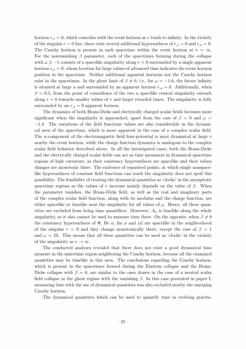
The dynamical quantities which can be used to quantify time in evolving gravita-

– 25 –

scalar field collapse in the Einstein theory

neutral [19] chargedD A D A

φ φ, q −

scalar field collapse in the Brans-Dicke theory

neutral [16] chargedD A D A

β = 0 Φ, φ (1) Φ, φ, q −β = 0.5 Φ, φ Φ, φ, qβ = 1 φ Φ, φ, q (2)

Table 1. Feasibility of using dynamical quantities of a coupled matter-geometry system to quantifytime nearby the singularity emerging during the gravitational evolution. The dynamical (v 6 20)and asymptotic (v → ∞) spacetime regions are denoted as D and A, respectively. The scalarand Brans-Dicke fields are φ and Φ, respectively, while q denotes the charge function (2.35).Notes: (1)except the vicinity of the Cauchy horizon for ω = −1.6, (2)except the asymptotic re-gion for ω = 10.

tional systems are gathered in table 1, which summarizes the investigations of potentialtime measurements nearby the singularities emerging during the collapse within the Ein-stein and Brans-Dicke theories. The outcomes of the research concerning the charged col-lapse in the Brans-Dicke theory support the conclusions about using dynamical quantitiesas time variables within the evolving spacetimes during dynamical gravitational evolutionsof coupled matter-geometry systems, which were formulated on the basis of investigatingthe neutral collapse in paper I. First, the spacelike character of the constancy hypersur-faces of the quantities and the monotonicity of their parametrization are not retained withinthe whole spacetime. Second, there does not exist a good time measure for the areas nearbythe Cauchy horizons. Third, in attempts to use dynamical quantities as ‘clocks’, specialattention should be paid to the values of the free evolution parameters, as they can stronglyinfluence this possibility.

In general, in comparison to the collapse of a neutral scalar field, the presence of the elec-tric charge in the spacetime modifies the feasibility of time quantification using the evolvingquantities in the following way. In the case of uncoupled Brans-Dicke and complex scalarfields, i.e., for β = 0, the charge spoils the possibility of measuring time with their use, whilewhen the fields are coupled, that is β is not equal to zero, the charge enhances it. In the stud-ied charged collapse, there also exist two more potential time measures, i.e., the chargefunction and the nonzero component of the Maxwell field four-potential. In the contextof time quantification, the former behaves analogously to the complex scalar field dynam-ical characteristics. On the other hand, the latter does not provide a good time measure,as its constancy hypersurfaces are timelike in the regions of high curvature.

During the gravitational collapse of an electrically charged scalar field, the mass infla-

– 26 –

tion phenomenon can appear in the spacetime. If so, a super-Planckian surface developsoutside the true singularity [9]. Within the region encompassed by it the spacetime curva-ture reaches values excluding the usage of a classical theory of gravity. Hence, quantizedgravity should be applied not around the singularity in this case, but around the massinflation super-Planckian surface. It is possible that in the vicinity of this hypersurface oneof the quantities discussed above or their combination could provide a good time measure.However, since the proposed construction depends on the cutoff of the super-Planckianregion, it requires more detailed studies on the region itself at first, as the determinationof its boundaries could be only arbitrary without any specific analyses. For this reason,we leave the announced topic for future researches.

Acknowledgments

A.N. was partially supported by the Polish National Science Center grant no. DEC-2014/15/B/ST2/00089. D.Y. is supported by Leung Center for Cosmology and Particle Astrophysics(LeCosPA) of National Taiwan University (103R4000).

A Numerical computations

The solution of the evolution equations (2.30), (2.33)–(2.37) was provided numerically withthe use of an enhanced version of the code prepared for the needs of paper I. The modulesgoverning the evolution of the gravitational, Brans-Dicke and scalar fields were modifiedin order to account for the presence of an electrically charged scalar field instead of a neutralone. The program was also supplied with a module governing the evolution of the Maxwellfield. The quantities Au and q were set as equal to zero along the initial v = 0 hypersurface,because due to the form of the evolving field, the center of the shell was not affected bymatter. The u-component of the electromagnetic field four-potential and the charge functionalong the initial u = 0 hypersurface were calculated according to (2.36) and (2.37).

The accuracy checks of the numerical code will be presented for a sample evolutionrunning for the parameters β = 0, ω = −1.4 and e = 0.3. The consistency of the computa-tions was monitored during all evolutions using the constraints (2.31) and (2.32). Figure 14presents the descendant quantities

Cons1 ≡2∣∣∣r,uu − 2fh+ r

2Φ (W,u − 2hW ) + rω2Φ2W

2 + 4πrΦ TEMuu

∣∣∣|r,uu|+

∣∣∣2fh− r2Φ (W,u − 2hW )− rω

2Φ2W 2 − 4πrΦ TEMuu

∣∣∣ , (A.1)

Cons2 ≡

∣∣∣r,vv − 2dg + r2Φ (Z,v − 2dZ) + rω

2Φ2Z2 + 4πr

Φ TEMvv

∣∣∣|r,vv|+

∣∣∣2dg − r2Φ (Z,v − 2dZ)− rω

2Φ2Z2 − 4πrΦ TEMvv

∣∣∣ , (A.2)

calculated along three arbitrary null hypersurfaces for the evolution with parameters spec-ified above. The values of Cons1 and Cons2 ought to be smaller than 2 in order to satisfythe constraints well (except the case when r,uu or r,vv vanishes). As can be inferred from

– 27 –

0 10 20 30 40 50 601E-6

1E-5

1E-4

1E-3

0.01

0.1

1

v

Cons1 u=5 Cons1 u=10 Cons1 u=15

Cons2 u=5 Cons2 u=10 Cons2 u=15

Figure 14. (color online) Monitoring of the constraints. The values of the equations (A.1) and (A.2)were calculated along three null hypersurfaces of constant u equal to 5, 10 and 15.

the plot, the error is less than 1% within almost the whole integration domain. Sincethe constraint equations are stable, the simulations are consistent.

The outcome of the convergence check of the numerical code for the sample evolutionis presented in figure 15. The values of a quantity constructed from the r function obtainedon two grids with a quotient of integration steps equal to 2 were calculated at three arbitraryu = const. hypersurfaces. An overlap between two profiles of the defined quantity at eachu = const. was obtained when the result from finer grids was multiplied by 4. Thus,the code displays a second order convergence. The discrepancy between each two profilesat each constant u hypersurface is less than 10−4% except a close vicinity of the singularity.

References

[1] B. S. DeWitt, Quantum theory of gravity. I. The canonical theory, Phys. Rev. 160 (1967)1113.

[2] S. Hod and T. Piran, Critical behavior and universality in gravitational collapse of a chargedscalar field, Phys. Rev. D 55 (1997) 3485.

[3] S. Hod and T. Piran, Mass inflation in dynamical gravitational collapse of a charged scalarfield, Phys. Rev. Lett. 81 (1998) 1554.

[4] S. Hod and T. Piran, The inner structure of black holes, Gen. Rel. Grav. 30 (1998) 1555.

[5] Y. Oren and T. Piran, Collapse of charged scalar fields, Phys. Rev. D 68 (2003) 044013.

[6] E. Sorkin and T. Piran, The effects of pair creation on charged gravitational collapse,Phys. Rev. D 63 (2001) 084006.

– 28 –

0 10 20 30 40 50 601E-12

1E-11

1E-10

1E-9

1E-8

1E-7

1E-6

1E-5

1E-4

1E-3

v

u=5, |r(0.5x0.5)-r(1x1)|/|r(0.5x0.5)|

u=5, 4|r(1x1)-r(2x2)|/|r(1x1)|

u=10, |r(0.5x0.5)-r(1x1)|/|r(0.5x0.5)|

u=10, 4|r(1x1)-r(2x2)|/|r(1x1)|

u=15, |r(0.5x0.5)-r(1x1)|/|r(0.5x0.5)|

u=15, 4|r(1x1)-r(2x2)|/|r(1x1)|

Figure 15. (color online) The convergence of the code presented through the prism of the valuesof the quantity |r(k×k) − r(2k×2k)|/|r(k×k)| with k = 0.5, 1 calculated at the same hypersurfacesof constant u as in figure 14. (k × k) denotes the resolution of the numerical grid, on whichthe computations were conducted.

[7] E. Sorkin and T. Piran, Formation and evaporation of charged black holes, Phys. Rev. D 63(2001) 124024.

[8] S. E. Hong, D. Hwang, E. D. Stewart, and D. Yeom, The causal structure of dynamicalcharged black holes, Class. Quant. Grav. 27 (2010) 045014.

[9] D. Hwang and D. Yeom, Internal structure of charged black holes, Phys. Rev. D 84 (2011)064020.

[10] A. Borkowska, M. Rogatko, and R. Moderski, Collapse of charged scalar field in dilatongravity, Phys. Rev. D 83 (2011) 084007.

[11] A. Nakonieczna and M. Rogatko, Dilatons and the dynamical collapse of charged scalar field,Gen. Rel. Grav. 44 (2012) 3175.

[12] A. Nakonieczna, M. Rogatko, and R. Moderski, Dynamical collapse of charged scalar fieldin phantom gravity, Phys. Rev. D 86 (2012) 044043.

[13] J. Hansen and D. Yeom, Charged black holes in string-inspired gravity: I. Causal structuresand responses of the Brans-Dicke field, JHEP 10 (2014) 040.

[14] J. Hansen and D. Yeom, Charged black holes in string-inspired gravity: II. Mass inflationand dependence on parameters and potentials, JCAP 09 (2015) 019.

[15] C.-Y. Zhang, S.-J. Zhang, D.-C. Zou, and B. Wang, Charged scalar gravitational collapse inde Sitter spacetime, Phys. Rev. D 93 (2016) 064036.

[16] A. Nakonieczna and D.-h. Yeom, Scalar field as an intrinsic time measure in coupleddynamical matter-geometry systems. I. Neutral gravitational collapse, Journal of High EnergyPhysics 02 (2016) 049.

– 29 –

[17] D. Hwang, H. Kim, and D. Yeom, Dynamical formation and evolution of (2+1)-dimensionalcharged black holes, Class. Quant. Grav. 298 (2012) 055003.

[18] A. Nakonieczna, M. Rogatko, and Ł. Nakonieczny, Dark sector impact on gravitationalcollapse of an electrically charged scalar field, Journal of High Energy Physics 11 (2015) 012.

[19] A. Nakonieczna and J. Lewandowski, Scalar field as a time variable during gravitationalevolution, Phys. Rev. D 92 (2015) 064031.

[20] E. Poisson and W. Israel, Internal structure of black holes, Phys. Rev. D 41 (1990) 1796.

[21] S. Hod and T. Piran, Late-time evolution of charged gravitational collapse and decay ofcharged scalar hair. I, Phys. Rev. D 58 (1998) 024017.

[22] S. Hod and T. Piran, Late-time evolution of charged gravitational collapse and decay ofcharged scalar hair. II, Phys. Rev. D 58 (1998) 024018.

[23] S. Hod and T. Piran, Late-time evolution of charged gravitational collapse and decay ofcharged scalar hair. III. Nonlinear analysis, Phys. Rev. D 58 (1998) 024019.

[24] D. Hwang, B. Lee, and D. Yeom, Mass inflation in f(R) gravity: A conjectureon the resolution of the mass inflation singularity, JCAP 1112 (2011) 006.

– 30 –