250
III. AFFECTED ENVIRONMENT

III. AFFECTED ENVIRONMENT


III.A. Affected Environment Gulf of Mexico
III-1
III. AFFECTED ENVIRONMENT
A. Gulf of Mexico
1. Geology The marine geology of the Gulf of Mexico region includes continental shelf, slope, borderlands (transitional continental to oceanic crust), and the abyssal plain areas. Detailed geologic reports of these planning areas are in U.S. Geological Survey (USGS) (1981), Jackson and Galloway (1984), Martin (1978), Gross (1993), and Geological Society of America (GSA) (2002). This section describes the geologic features and processes associated with seafloor instabilities. Seafloor instabilities can result in damage to offshore infrastructure that could result in environmental impacts. For information on general petroleum geology, refer to The Resource Evaluation Program Structure and Mission on the Outer Continental Shelf (Dellagiarino and Meekins, 1998). For additional information on the geologic and petroleum geology of the different Outer Continental Shelf (OCS) planning areas in the Gulf of Mexico Region, refer to Minerals Management Service (MMS) (2002a, 2003c). The MMS Environmental Studies Program has conducted studies in areas where more detailed geologic information was needed for management of the OCS minerals leasing program. These studies have provided assessments of operational constraints to oil and gas exploration and production. The data and mapped information are being used on a daily basis for tract evaluation, lease stipulation development and application, protection of sensitive areas such as the Flower Garden Banks, and reviewing exploration, development, pipeline, and structure decommissioning applications. Seafloor stability and movements are often influenced by oceanographic processes acting either at the sea surface through ocean-atmosphere interactions that occur during extreme weather events, such as hurricanes and frontal cyclones, or at depth in association with currents involved in the circulation of the Gulf of Mexico, such as the Loop Current and associated eddies. The sections that follow on meteorology and physical oceanography provide more information on the interactions between the atmosphere-ocean system and geologic hazards.
a. Physiography The Gulf of Mexico is composed of two broad physiographic regional provinces: the continental margin and the ocean-basin floor. The continental margin includes two sub-provinces; the continental shelf and continental slope. The continental shelf is the submarine extension of the coastal plain deposits from the shoreline to about the 200-meter (m) water depth and is characterized by a gentle slope of a few meters per kilometer (less than one degree). In the eastern part of the Gulf, the adjacent continental slope extends from the shelf edge to the Sigsbee and Florida Escarpments, in about 2,000- to 3,000-m water depths. In the northwestern Gulf, the continental slope consists of two parts: the gently sloping upper slope with its characteristic hummocky topography due to diapiric salt structures, and the relatively steep topography of the lower slope. The transitional zone between the continental shelf and slope is an area of potential geologic hazards due to differences in seafloor stability (MMS, 2002a; USGS, 1981). The deep ocean-basin floor includes the continental rise and the abyssal plain provinces. The continental rise is a gently sloping depositional feature that extends from the base of the continental slope to the abyssal plain. The sediments comprising the continental slope were transported from the continents by bottom currents, gravitational creep, and turbid flow down submarine canyons. That

III.A. Affected Environment Gulf of Mexico
III-2
abyssal plain is an essentially flat-lying sequence of thick sediments deposited in a deep-ocean environment where water depths are more than 3,350 m (MMS, 2002a; USGS, 1981).
b. General Environmental Geology and Geologic Hazards Within the Gulf of Mexico Region, naturally-occurring processes and other surface and subsurface geologic features could cause seafloor instabilities that may become major geologic hazards to oil and gas development. Thick sequences of sediments have been deposited on the continental margin and ocean basin via bottom currents, gravitational creep, slumps, and turbidity or debris flows. Within the Gulf of Mexico, these naturally-occurring processes may become major geologic hazards to oil and gas development. Seafloor instability is considered the principle engineering constraint to the emplacement of bottom-founded structures, including pipelines, drilling rigs, and production platforms. A description of the major geologic processes that could result in seafloor instability follows. Bed Form Migration: Several types of bed forms are present in the Gulf of Mexico ranging from giant bed forms to small-scale ripples and sand waves. Bed form migration is of particular significance in the eastern Gulf of Mexico. The structural integrity of offshore facilities could be affected by the movement of these bed forms. The size, shape, and orientation of bed forms are affected by the oceanographic processes that form them. Megafurrows: Recent surveys conducted by Texas A&M University on the lower continental slope of the Gulf of Mexico have confirmed that deepwater processes have produced megafurrows parallel to the bathymetric contour lines southward of the Sigsbee Escarpment. These large bed forms, 20-30 m wide and as deep as 10 m, occur along the base of the Sigsbee Escarpment and extend to a distance of 20 kilometers (km) south of the escarpment. These megafurrows suggest swift bottom currents in water depths of over 3,000 m along the base of the escarpment (Bryant and Liu, 2000). Shallow Waterflow: Shallow waterflow, also known as geopressured sands, is the uncontrolled flow of sand and water that can create sediment accumulation at the wellhead. This process is the result of compaction, disequilibrium, or differential compaction and usually occurs at 360-530 m below the seafloor. It is more likely to occur on the upper and middle slope and less likely to occur above the salt nappe, the tabular salt blocking the escape of overpressures from below (MMS, 2000). Slope Stability: Two factors control the near-surface submarine slope stability of the continental margins offshore from Texas and Louisiana: (1) interplay between episodes of rapid shelf edge progradation and contemporaneous modification of the depositional sequence by diapirism, and (2) mass movement processes. Sediment instability is more likely to occur on the continental slope because of the relatively steep gradients. In addition, rapid deposition of sediment at the shelf edge, cyclic loading of storm waves, faulting, and vertical migration of shallow salt create further instabilities. These local high rates of deposition of unconsolidated sediments on the continental shelf edge form unstable slopes that lead to intensive soil movements such as slumping, gravitational creep, turbidity or debris flows, and mudslides. Many slope sediments have been uplifted, folded, fractured, and faulted by diapiric action creating oversteepened slopes that also lead to slope failures. Some intraslope basins contain fill sequences of repeated and stacked chaotic units that are interpreted as the products of massive failures. These deposits likely originated at or near the shelf edge during periods of lowered sea level and failed during the sediment loading process. Oversteepening on the basin flanks and resulting mass movements have created highly overconsolidated sediments underlying extremely weak pelagic sediments (MMS, 2000).

III.A. Affected Environment Gulf of Mexico
III-3
A wide range of failure features results from the mass movements of sediment, from massive shelf edge evacuation features (Winker and Edwards, 1983 as cited in Louisiana State University, Coastal Marine Institute [LSU CMI], 2001) to small-scale slumps along fault faces and on the sides of diapirs. Depending on scale, massive volumes of sediment can be transported downslope in association with subaqueous mass movement processes (Coleman et al. 1986 as cited in LSU CMI, 2001). The principal types of sediment mass movements that occur along the Gulf of Mexico shelf are surface mudflows and slumps. Surface mudflows most typically develop in the Mississippi Delta area off the mouths of the principal passes that empty into the Gulf. Downslope advance of these features is characterized by glacierlike flow of soft soil over the seafloor that may be either continuous or intermittent. These features are usually less than 15 m thick and form noses or scarps at their leading edges up to 15 m in height. Slumps typically occur within the upper 15 m of sediment and subparallel to the bathymetric contours. They are characterized stairstep-like faulting that decrease in steepness with depth (USGS, 1981). The upper continental slope is subdivided into several areas based on the various types of seafloor and slope instability (MMS, 1989a, b; 1990a, b; and 1991a). These areas are depicted and described in Figure III-1. Active Faulting: Faulting occurs on many scales along the continental slope, from major growth faults that cut across thousands of meters of sedimentary section to much smaller faults related primarily to salt movement in the shallow subsurface (LSU CMI, 2001). Faults are most common (1) in areas of rapid deposition, such as the Mississippi Delta, (2) in areas that are rapidly subsiding due to withdrawal of formation fluids such as water and oil, (3) along steep slopes where stress due to sediment loading is relieved by sudden faulting, (4) along the shelf edge where slope steepening (increased gradient) occurs at the edge of the continental shelf as it merges with the continental slope, and (5) on active diapers on the upper slope (USGS, 1981). The large regional systems of growth faults are associated with massive sediment accumulation. They formed contemporaneously with sedimentation, resulting in throws of thousands of feet that increase with depth (Jackson and Galloway, 1984). The growth faults are found mostly on the upper continental slope and on the continental shelf where sediment accumulation is the thickest. They parallel the coastline and penetrate into the Cenozoic units beneath coastal Texas and Louisiana and the adjacent shelf. Growth faults and smaller-scale faults are responsible for offsetting the seafloor and creating local steep slopes that can lead to various forms of mass movement. Surface and subsurface convex faults are similar in nature to the growth faults (above) in that they may posses subsurface offsets of 6 m (20 ft) or more, and may extend to depths of more than 152 m (500 ft) below the mudline. They typically extend to or very near the surface where scarps may form. Faulting associated with active diapirism create small escarpments on the seafloor. This type of faulting, which is common in the Gulf of Mexico, can be active within the lifetime of oil and gas fields (USGS, 1981). In addition, faults are responsible for numerous constructional seafloor features related to the vertical flux of fluids and gases and expulsion of these products at the ocean bottom. At one end of the feature spectrum are large mud volcanoes (Neurauter and Bryant, 1990; Neurauter and Roberts, 1994 as cited in LSU CMI, 2001) formed by fine-grained sediment forced up along the faults. At the other end of the spectrum, vertical flux of gases and fluids may be very slow. Shallow Gas: Gas seeps and shallow gas accumulations in the near-surface sediments commonly occur in the shelf-depth areas of the northern Gulf. Decomposition of trapped organic matter within the upper few tens of meters of sediment is the primary source of biogenic gas. Thermogenic gas, originating in deeply buried source rocks, can migrate upward, especially along fault planes and also become trapped in shallow sediments. Typically, most seeps are ephemeral, existing only long enough to relieve an overpressured accumulation; however, seeps rising along faults from deeper

III.A. Affected Environment Gulf of Mexico
III-4
reservoirs may be semi-permanent (MMS, 1989a, b; 1990a, b; and March 1991a). Along the Texas-Louisiana shelf, shallow gas accumulations are most common in old channel systems as well as areas affected by salt uplift where numerous faults form passageways to near-surface sediments forming small gas pockets sealed in thin clay layers. Along the Mississippi Delta, shallow gas is predominantly biogenic (USGS, 1981). The occurrence of gas of either origin (biogenic or thermogenic) may be hazardous under certain conditions. Violent blowouts have resulted from drilling into high-pressure accumulations only a few hundred meters below the mudline. Drilling into areas of rapid deposition with associated biogenic gas, such as active deltas, can pose problems since a large amount of gas can lower the density of the mud and can contribute to seafloor instability and slope failure. This occurs when methane is generated in sediment pore waters that exceed saturation such that gas bubbles form resulting in increased pore pressure that may lower sediment shear strengths to the point of failure. This process is believed to have contributed to past pipeline ruptures and platform failures around the Mississippi Delta (MMS, 1989a, b; 1990a, b; and 1991a). Natural Gas Hydrates: Formation of gas hydrates, ice-like crystalline solids formed by low-molecular-weight hydrocarbon gas molecules (mostly methane), in deepwater operations is a well-recognized and potentially hazardous operational problem in water depths greater than 300 m. Seabed conditions of high pressure and low temperature become conducive to gas hydrate formation in deep water. Because of the strong fault-related vertical flux of both gas and water to the seafloor (described above), gas hydrates are able to exist at or near the sea floor in water depths greater than about 500 m. The process of vertical flux of water and gas up faults produces mound-like accumulations; however, hydrates most commonly occur below the surface with an overlying and insulating layer of fine-grained sediment (MMS, 2002a; LSU CMI, 2001). The primary gas hydrate hazards issues include drilling difficulties caused by sediments that may contain hydrates, hydrate blockages inside pipes, pressure build up inside pipes, the risk of blowouts, and seafloor stability issues associated with loss of soil strength when hydrates become dissociated (Boatman and Peterson, 2000).
2. Meteorology and Air Quality a. Climate The Gulf of Mexico is influenced by a maritime subtropical climate controlled mainly by the clockwise wind circulation around a semipermanent, high barometric pressure area alternating between the Azores and Bermuda Islands. The circulation, around the western edge of the high pressure cell results in the predominance of moist southeasterly wind flow in the region. During the winter months, December through March, cold fronts associated with outbreaks of cold, dry continental air masses influence mainly the northern coastal areas of the Gulf of Mexico. Tropical cyclones may develop or migrate into the Gulf of Mexico during the warmer season, especially in the months of August through October. In coastal areas, the land-sea breeze is frequently the primary circulation feature in the months of May through October. In the warmest month in the summer, average temperatures in the Gulf coastal areas range from about 26 to 28 degrees Celsius (°C) (79 to 82 degrees Fahrenheit [°F]). During the warm months, there is little diurnal, daily or spatial variation in temperature. Average temperatures for the coldest month in winter range from about 10 °C (50 °F) in the northern coastal areas to about 21 °C (70 °F) in the

III.A. Affected Environment Gulf of Mexico
III-5
southernmost locations in Texas and Florida. In the colder months, there is more variability in temperature, mainly in the more northern areas. Air temperatures over the open Gulf exhibit smaller daily and seasonal variations due to the moderating effects of large bodies of water. The average temperature over the center of the Gulf is about 29 °C (84 °F) in the summer and between 17 and 23 °C (63° and 73 °F) in the winter. The relative humidity over the Gulf and the coastal areas is high, especially during the warmer months. Lower humidities in the winter season are associated with outbreaks of cool, dry, continental air from the interior. Winds are generally southeasterly to southerly in the summer season, but are more variable in the coastal regions because of effects of the land-sea breeze circulation systems. Winds are more changeable in the winter season because of changing atmospheric pressure patterns and frontal passages. Precipitation is frequent and abundant throughout the year, but tends to peak in the summer months. Mean annual rainfall ranges from about 77 centimeters (cm) (30 inches) along parts of the Texas Gulf Coast to 155 cm (60 inches) in the Florida Panhandle. Rainfall in the warmer months is usually associated with convective cloud systems that produce showers and thunderstorms. Winter rains are associated with the passage of frontal systems through the area. Fog occurs occasionally in the cooler season as a result of warm, moist Gulf air blowing over cool land or water surfaces. The poorest visibility conditions occur from November through April. During air stagnation, industrial pollution and agricultural burning also can impact visibility. Atmospheric stability and mixing height provide a measure of the amount of vertical mixing of pollutants. Over water, the atmosphere tends to be neutral to slightly unstable since there is usually a positive heat and moisture flux. Over land, the atmospheric stability is more variable, being unstable during the daytime, especially in the summer months due to rapid surface heating, and stable at night, especially under clear conditions in the cooler season. The mixing height over water typically ranges between 500 m and 1,000 m with a slight diurnal variation. Mixing height over land can be 1,500 m or greater during the afternoon in the summertime and near zero during clear, calm conditions at night in the wintertime. Tropical cyclones affecting the Gulf originate over the tropical portions of the Atlantic Ocean, the Caribbean Sea, and the Gulf of Mexico and occur most frequently between June and September. On average, about 10 tropical cyclones occur in the Atlantic Basin, 5 of which become major hurricanes. About 3.7 tropical cyclones per year will affect the Gulf of Mexico (MMS, 1988b). Tropical storms cause damage to physical, economic, biological, and social systems in the Gulf, but the severest effects tend to be highly localized. The Gulf of Mexico is also periodically affected by wintertime, extratropical cyclones generated when continental, cold air outbreaks interact with the warm Gulf waters. These storms can produce gale force winds and high seas, and are hazardous to shipping due to their sudden and rapid formation. For effects of hurricanes and severe storms on OCS oil operations in the Gulf, see the 5-Year Final Environmental Impact Statement for the Outer Continental Shelf Oil & Gas Leasing Program: 2002-2007 (MMS, 2002c: sec. 4.1.4.5).
b. Air Quality Air quality of the coastal areas bordering the Gulf of Mexico can be described by comparing measured ambient concentrations of pollutants against the national ambient air quality standards (NAAQS) established by the U.S. Environmental Protection Agency (USEPA) under the Clean Air Act. The NAAQS have been established for the so-called criteria pollutants, which are nitrogen dioxide (NO2), sulfur dioxide (SO2), particulate matter less than 10 microns in diameter (PM10), fine particulates less

III.A. Affected Environment Gulf of Mexico
III-6
than 2.5 microns in diameter (PM2.5), carbon monoxide (CO), and ozone (O3). Any individual State may adopt a more stringent set of standards. The State of Florida has ambient standards for SO2 that are somewhat more stringent than the NAAQS. All of the Gulf coastal counties meet the NAAQS for NO2, SO2, CO, PM10, and PM2.5. However, the O3 standard is exceeded in a number of counties in Texas and Louisiana. Figure III-2 shows the areas that are classified nonattainment for O3. There are ten counties in the Houston, Galveston, Beaumont, and Port Arthur metropolitan areas in southeastern Texas that do not meet the Federal standards for O3. The USEPA has established four categories of O3 nonattainment areas: marginal, moderate, serious, and severe. The seven counties around Houston and Galveston are classified severe. The three counties in the Beaumont and Port Arthur areas are classified serious. During the monitoring period of 2002 through 2004, the highest 1-hour average O3 concentration in Houston was 230 parts per billion (ppb). There was an average of about 7 days per year when the O3 standard was exceeded in the Houston metropolitan area. In the Beaumont-Port Arthur area, there were no exceedances of the 1-hour O3 standard in the 2002 through 2004 period. On June 15, 2004, the USEPA issued their list of area designations with respect to the new 8-hour average O3 standard. The Houston-Galveston metropolitan area was designated nonattainment with a moderate severity rating. The Beaumont-Port Arthur area was classified nonattainment with a marginal rating. In Louisiana, five parishes in the Baton Rouge area are classified nonattainment for O3. The five Baton Rouge parishes are classified in the serious category. In the 2002-2004 monitoring period, the highest 1-hour average O3 concentration was 160 ppb. There is an average of about 2-3 days per year when the Federal O3 standard is exceeded. The Baton Rouge area is a marginal nonattainment area with respect to the 8-hour O3 standard. Coastal areas of Mississippi, Alabama, and Florida are classified attainment for O3. The largest sources of nitrogen oxide (NOx) emissions are vehicles and electric utilities. Other important sources are nonroad engines and vehicles and industrial plants. In southeastern Texas and southern Louisiana, petroleum refining and chemical plants provide a substantial contribution to volatile organic compound (VOC) emissions. Other important sources are solvents (industrial solvents, paints, consumer solvents, dry cleaning), vehicles, nonroad engines and vehicles, and petroleum storage and transport. Class I Federal areas have been designated for mandatory Prevention of Significant Deterioration (PSD) of air quality, including such air-quality-related values as visibility. The PSD Class I areas are located in two of the five Gulf Coast States: Louisiana and Florida. In Louisiana there is one Class I area, and Florida has three. The Class I area offshore Louisiana is comprised of the Breton Wildlife Refuges, located on Breton Island and on many of the Chandeleur Islands. Figure III-3 shows the locations of the Class I areas in the Gulf coastal zones.
3. Physical Oceanography The Gulf of Mexico is connected to the Caribbean Sea and the Atlantic Ocean via the Yucatan Channel and the Florida Straits, respectively. The Loop Current, the dominant circulation feature in the Gulf, enters through the Yucatan Channel and exits through the Florida Straits (Fig. III-4). The sill depth at the Florida Straits is about 800 m. Because the sill depth at the Yucatan Channel is less than

III.A. Affected Environment Gulf of Mexico
III-7
1,800 m, water masses in the Atlantic Ocean and Caribbean Sea that occur at depths exceeding this cannot enter the Gulf of Mexico. The Loop Current dominates circulation in the Gulf of Mexico. A typical location is presented in Figure III-4. The extent of intrusions of the Loop Current into the Gulf of Mexico varies and may be related to the location of the current on Campeche Bank at the time it separates from the bank. Filaments of the Loop Current have been observed to intrude onto the continental slope east of the Mississippi River Delta. Another Loop Current associated circulation feature is anticyclonic Loop Current eddies, which are closed, clockwise rotating rings of water that separate from the Loop Current. Major Loop Current eddies have diameters on the order of 300-400 km and may extend vertically to a depth of about 1,000 m. Once these eddies are free from the Loop, they travel into the western Gulf along various paths to a region between 25o N. to 28o N. latitude and 93o to 96o W. longitude. It is thought that separation of these eddies from the Loop Current occurs aperiodically. Eddies can have lifetimes exceeding 1 year (Elliott, 1982). Currents associated with the Loop Current and its eddies can have surface speeds of 150-200 centimeters per second (cm/s) or more; speeds of 300 cm/s have been observed. At depth of 500 m, speeds of 10 cm/s can occur (Cooper et al., 1990). Exchange of surface and deep water occurs with descent of surface water beneath the Loop Current in the eastern Gulf of Mexico, and with the ascent of deep water in the northwestern Gulf of Mexico where Loop Current eddies spin down (Welsh and Inoue, 2002). In addition to currents associated with the Loop Current and associated mesoscale eddies, there are two other significant circulation features in the Gulf of Mexico (Fig. III-4). One is a permanent anticyclonic (clockwise rotating) feature oriented about ENE-WSW with its western extent near 24° N. latitude off Mexico. The causal mechanism for this anticyclonic circulation and the associated western boundary current along the coast of Mexico is debatable (Sturges and Blaha, 1975; Elliott, 1979, 1982; Blaha and Sturges, 1981; Sturges, 1993) but is suspected to be wind-driven (Oey, 1995). The second feature is a cyclonic gyre centered in the Bay of Campeche near 20.8° N. latitude, 94.5° W. longitude (Vazquez de la Cerda, 1993). This circulation feature is also thought to be wind-driven (Nowlin et al., 2000). Shelf circulation is complicated because of the large number of forces and seasonality of driving forces. Cochrane and Kelly (1986) examined the prevailing circulation on the Texas-Louisiana continental shelf. With the exception of July-August, there appears to be a cyclonic (rotating counter-clockwise) gyre present over this part of the northern Gulf of Mexico continental shelf in response to prevailing wind stress (Fig. III-4). On the inner shelf, currents flow down the coast (west-southwestward). A corresponding countercurrent, which completes the gyre system, occurs along the shelf break. At the southwestern end of the gyre, the convergence migrates seasonally with the direction of the prevailing wind, ranging from a point south of the Rio Grande in the fall to the Cameron area by July. In July, the cyclonic system is replaced by an anticyclone (rotating clockwise) offshore Louisiana, which has formed in response to the up-the-coast component of the wind. In August and September, the direction of the prevailing winds change to down the coast, and the cyclonic gyre is reestablished. Circulation on the Mississippi-Alabama shelf is dynamic because a number of factors are involved, including the Loop Current and associated intrusions, tides, winds, and freshwater inflow. Kelly (1991) reported results from current meter moorings that agreed with a mean cyclonic circulation cell as suggested by Dinnel (1988), and stating that the wind-driven flow on the inner shelf was westward and that the return eastward flow occurred over the mid- and outer shelf (Fig. III-4). Three types of intrusions have been identified: (1) Loop Currents push up the axis or east side of De Soto Canyon, (2) frictional entrainment of outer shelf water into the outer periphery of the Loop Current or an eddy

III.A. Affected Environment Gulf of Mexico
III-8
filament derived from the Loop Current, and (3) direct intrusion of diluted Loop Current water onto the shelf. These phenomena can markedly alter the general wind-driven circulation of the continental shelf. Because the intrusions are random, frequent, strong, and have variable areal coverage, they are an important influence on the circulation in this region. The flow structure on the west Florida continental shelf consists of three regimes: the outer shelf, the mid-shelf, and the coastal boundary layer. The Loop Current and eddy-like perturbations more strongly affect the circulation on the outer shelf. During Loop intrusion events, upwelling of colder, nutrient-rich waters has been observed. In water depth less than 30 m, the wind-driven flow is mostly alongshore and parallel to the isobaths. A weak mean flow is directed southward in the surface layer. In the coastal boundary layer, longshore currents driven by winds, tides, and density gradients predominate over the cross-shelf component (Science Applications International Corporation, 1986). Deepwater circulation is influenced by the Loop Current, eddies, permanent gyres, and several additional types of currents. Loop Current eddies and their interaction with the shelf can cause the formation of deep eddies (Frolov et al., 2004). A cyclonic deep mean flow exists around the edges of the entire Gulf at about a 2000-m depth (Sturges et al., 2004). There are deep barotropic currents; subsurface-intensified, high-speed jets; and a class of deep currents that was detected by documenting their effects in producing long, deep, linear furrows in the bottom sediments near the Sigsbee Escarpment. In deep water, barotropic (depth independent) currents have been observed to extend from depths near 1,000 m to the bottom. Barotropic currents have been observed with maximum speeds near 70 cm/s and lasting for periods of weeks (Hamilton et al., 2003). Very high-speed, subsurface-intensified currents lasting of the order of a day have been observed at locations over the upper continental slopes (DiMarco et al., 2004). These currents may have vertical extents of less than 100 m, with maxima observed generally within the depth range of 100-300 m, and maximum speeds exceeding 150 cm/s. In early 1999, previously unexplored bed forms were discovered just offshore of the Sigsbee Escarpment in the northwestern Gulf of Mexico by Dr. William Bryant of Texas A&M University. These consisted of large, megafurrows eroded into the seafloor, oriented nearly along depth contours, and having depths of 5-10 m and widths of several tens of meters. They are spaced on the order of 100 m apart, and extend unbroken for distances of tens of kilometers or more. The presence of these megafurrows suggests the presence of bottom currents that have along-isobath components and increase in strength toward the escarpment. These currents might be sporadic or quasi-permanent, and near-bottom speeds might be 50 cm/s or even in excess of 100 cm/s.
4. Water Quality The definition of water quality in this environmental impact statement is the ability of a water body to maintain the ecosystems it supports or influences under natural conditions. This definition includes human uses of water for recreation, food harvest, and industrial and domestic uses. This description divides the analysis area into coastal and marine waters. Coastal waters include all the bays and estuaries from the Rio Grande River to the Florida Bay. Marine water includes both State offshore water and Federal OCS waters extending from outside the barrier islands to the Exclusive Economic Zone. The inland extent is defined by the Coastal Zone Management Act. A further subdivision within the marine water areas is between continental shelf water and deep water. In general, coastal water quality is influenced by the rivers that drain into the area, the quantity and composition of wet and dry atmospheric deposition, and the influx of constituents from sediments.

III.A. Affected Environment Gulf of Mexico
III-9
Human activities influence the waters closest to the land. Circulation or mixing of the water may either improve the water through flushing or degrade the quality by introducing factors that contribute to water quality decline. Marine water composition in the Gulf of Mexico has two primary influences. These are the configuration of the Gulf of Mexico Basin, which controls the oceanic waters that enter and leave the Gulf, and runoff from the land masses, which controls the quantity of freshwater input into the Gulf. The Gulf of Mexico receives oceanic water from the Caribbean Sea through the Yucatan Channel, and freshwater from major continental drainage systems such as the Mississippi River system. The large amount of freshwater runoff mixes into the Gulf surface water, producing a composition on the continental shelf that is different from the open ocean.
a. Coastal Waters The Gulf Coast contains one of the most extensive estuary systems in the world. This system extends from the Rio Grande River in Texas eastward to Florida Bay in Florida. Estuaries are semienclosed basins within which the freshwater of rivers and the higher salinity waters offshore mix. Estuaries are influenced by both freshwater and sediment influx from rivers and the tidal actions of the oceans. The primary variables that influence coastal water quality are water temperature, total dissolved solids (salinity), suspended solids (turbidity), and nutrients. An estuary’s salinity and temperature structure is determined by hydrodynamic mechanisms governed by the interaction of marine and terrestrial influences. Hydrodynamic influences include tides, nearshore circulation, freshwater discharges from rivers, and local precipitation. Tidal mixing within Gulf estuaries is limited by the small tidal ranges that occur along the Gulf of Mexico coast. The shallowness of most Gulf estuaries, however, tends to amplify the mixing effect of the small tidal range. Gulf Coast estuaries exhibit a general east to west trend in selected attributes of water quality associated with changes in regional geology, sediment loading, and freshwater inflow. For example, the estuarine waters in Florida generally have greater clarity and lower nutrient concentrations than those in the central and western areas of the Gulf Coast. The primary factors that affect estuarine water quality include upstream withdrawals of water for agricultural, industrial, and domestic purposes; contamination by industrial and sewage discharges; agricultural runoff carrying fertilizer, pesticides and herbicides; upstream land use; and habitat alterations (e.g., construction and dredge and fill operations). Because drainage from more than 55 percent of the conterminous United States enters the Gulf of Mexico primarily from the Mississippi Rive, a large area of the nation contributes to coastal water quality conditions in the Gulf. Population growth results in additional clearing of the land, excavation, construction, expansion of paved surface areas, and drainage controls. These activities alter the quantity, quality, and timing of freshwater runoff. Storm water runoff which flows across impervious surfaces is more likely to transport contaminants associated with urbanization including suspended solids, heavy metals and pesticides, oil and grease, and nutrients (U.S. Commission on Ocean Policy, 2004). Additional information on factors that contribute to coastal water quality can be found in the Sociocultural Systems section of this chapter. Coastal water quality is also affected by the loss of wetlands which is discussed in detail in the Coastal Habitats section of this chapter. Wetlands improve water quality through filtration of runoff water and provision of valuable habitat. Suspended particulate material is trapped and removed from the water resulting in greater water clarity. Nutrients may also be incorporated into vegetation and removed from the water that passes through the wetlands.

III.A. Affected Environment Gulf of Mexico
III-10
Current Status of Gulf of Mexico Coastal Water Quality: The first USEPA National Coastal Condition Report summarized coastal conditions with data collected from 1990-1996 (USEPA, 2001). The USEPA has updated this information in a second report (USEPA, 2004a). The Gulf of Mexico coastal area was rated fair to poor in the first report. The primary reasons for this rating were the areal extent of contaminated sediments, wetland losses, poor benthic conditions, and the high expression of eutrophic condition. The ranking method was changed between reports, so comparisons are difficult. The second report ranked the water quality index and the overall condition fair. The ranking used five factors: (1) dissolved oxygen, (2) dissolved inorganic nitrogen (3) dissolved inorganic phosphorus, (4) chlorophyll a, and (5) water clarity. Estuaries with a poor water-quality rating comprised 9 percent of the Gulf Coast estuaries while those ranked fair to poor comprised 51 percent. In Texas and Louisiana, the estuaries that received a poor water-quality rating in the report had low water clarity and high dissolved inorganic phosphorus levels in comparison to those expected for that region. The factors that contributed to a poor water-quality rating in Florida and Mississippi estuaries were low water clarity and high chlorophyll relative to expected levels. Chlorophyll is one of several symptoms of eutrophic conditions. Dissolved oxygen levels in Gulf Coast estuaries are good, and less than 1 percent of bottom waters exhibit hypoxia (dissolved oxygen level below 2 milligrams per liter (mg/L)). Sediments can serve as a sink for contaminants that were originally transported via water in either dissolved or particulate form or via atmospheric deposition. Sediments may contain pesticides, metals, and organics. The sediments of Gulf Coast estuaries were ranked as fair. Metals were the type of sediment contamination found to most frequently exceed toxicity guidance. Some species of estuarine and marine fish contain mercury. Although very small amounts of mercury enter the coastal environment from a range of sources, mercury concentrates in the tissue of predatory fish species. State and Federal Agencies publish guidance which describes the species of fish that should be eaten in limited quantities. The USEPA merged both State and Federal mercury data into the Gulfwide Mercury in Tissue Database to characterize the occurrence of mercury in fishery resources (Ache, 2000). The reports found that all Gulf Coast States have published fish consumption advisories for large king mackerel. A gulfwide coordinated sampling program is underway to characterize mercury levels for additional estuarine and marine species.
b. Marine Waters Within the Gulf of Mexico, marine waters occur in three regions: (1) the continental shelf west of the Mississippi River, (2) the continental shelf east of the Mississippi River, and (3) deep water (>305 m).
(1) Continental Shelf West of the Mississippi River The Mississippi and Atchafalaya Rivers are the primary sources of freshwater, sediment, and pollutants to the continental shelf west of the Mississippi (Murray, 1997). The Mississippi–Atchafalaya River Basin drains about 41 percent of the conterminous United States (Committee on Environment and Natural Resources, 2000). While the average river discharge from the Mississippi River exceeds the input of all other rivers along the Texas-Louisiana coast by a factor of 10, during low-flow periods, the Mississippi River can have a flow less than all the other rivers combined (Nowlin et al., 1998). The water quality in this area is highly influenced by input of sediment and nutrients from the Mississippi and Atchafalaya Rivers. A turbid surface layer of suspended particles is associated with the freshwater plume from these rivers. The river system supplies nitrate, phosphate, and silicate to the shelf. During summer months, the low-salinity water from the Mississippi River

III.A. Affected Environment Gulf of Mexico
III-11
spreads out over the shelf, resulting in a stratified water column. While surface oxygen concentrations are at or near saturation, hypoxia, defined as oxygen concentrations less than 2 mg/L, is observed in bottom waters during the summer months (Fig. III-5). The Hypoxic Zone: The hypoxia zone on the Louisiana-Texas shelf is one of the largest of the 150 oxygen deprived zones that occur throughout the world (United Nations Environment Programme, GlobalEnvironmentOutlook, GEOYearbook 2002––http://www.unep.org/geo/yearbook/089.htm). From 1985-1995 and 1993-1999, the area of hypoxia covered 8,000-9,000 square kilometers (km2) and 16,000-20,000 km2, respectively (Committee on Environment and Natural Resources, 2000). Three phenomena are occurring within the drainage basin that are related to the appearance and growth of the hypoxic zone: (1) landscape alteration through deforestation and artificial agricultural drainage, (2) river channelization and (3) increased use of fertilizer. The oxygen-depleted bottom waters occur seasonally and are affected by the timing of the Mississippi and Atchafalaya Rivers’ peak discharges that carry nutrients to the surface waters. This, in turn, increases the carbon flux to the bottom, which, under stratified conditions, results in hypoxic oxygen depletion (oxygen concentration <2 mg/L). The variables that control the timing of the event include stratification, weather patterns, temperature, and precipitation in the Gulf and in the drainage basin. The hypoxic conditions persist until local wind-driven circulation mixes the water again. Organic Pollutants: Analysis of shelf waters and sediments off the coast of Louisiana will occasionally detect trace organic pollutants including polynuclear aromatic hydrocarbons (PAH), herbicides such as Atrazine, chlorinated pesticides, and polychlorinated biphenyls (PCB), and trace inorganic (metals) pollutants, for example, mercury. The concentrations of chlorinated pesticides and PCB’s, which are associated with suspended particulates and sediment, continue to decline since their use has been discontinued. The source of these contaminants is the river water that feeds into the area. In sediment cores collected in water from 10-100 m off of the southwest pass of the Mississippi River, the detection of organochlorine pesticides and PAH’s increased in sediments dated post-1940’s. The river was identified as the source of both organochlorine and the pyrogenic PAH’s (Turner et al., 2003).
(2) Continental Shelf East of the Mississippi River Water quality on the continental shelf from the Mississippi River Delta to Tampa Bay is influenced by river discharge, runoff from the coast, and eddies from the Loop Current. The Mississippi River accounts for 72 percent of the total discharge onto the shelf (SUSIO [State University System of Florida Institute of Oceanography], 1975). The outflow of the Mississippi River generally extends only 75 km (45 miles) to the east of the river mouth (Vittor and Associates, Inc., 1985) except under extreme flow conditions. The Loop Current intrudes in irregular intervals onto the shelf, and the water column can change from well mixed to highly stratified very rapidly. Discharges from the Mississippi River can be easily entrained in the Loop Current. The flood of 1993 provided an infusion of fresh water to the entire northeastern Gulf of Mexico shelf with some Mississippi River water transported to the Atlantic Ocean through the Florida Straits (Dowgiallo, 1994). Hypoxia is rarely observed on the Mississippi-Alabama shelf, although low dissolved oxygen values of 2.93-2.99 mg/l were observed during the MAMES cruises (Brooks, 1991). The Mississippi-Alabama shelf sediments are strongly influenced by fine sediments discharged from the Mississippi River. The shelf area is characterized by a bottom nepheloid layer and surface lenses of suspended particulates that originate from river outflow. The West Florida Shelf receives very little

III.A. Affected Environment Gulf of Mexico
III-12
sediment input. The water clarity is higher towards Florida, where the influence of the Mississippi River outflow is rarely observed. Red Tides: Red tides, which are blooms of single-cell algae that produce potent toxins harmful to marine organisms and humans and are a natural phenomenon in the Gulf of Mexico, occur primarily off southwestern Florida and Mexico. These algal blooms can result in severe economic and public health problems, and are responsible for fish kills and invertebrate mortalities. There are ongoing studies to determine whether human induced nutrient loadings contribute to the frequency and intensity of these red tides. Baseline Conditions: A 3-year, large-scale marine environmental baseline study conducted from 1974 to 1977 in the eastern Gulf of Mexico resulted in an overview of the Mississippi, Alabama, and Florida (MAFLA) OCS environment out to 200 m (SUSIO, 1977; Dames and Moore, 1979). Analysis of water, sediments, and biota for hydrocarbons indicated that the MAFLA area is pristine, with some influence of anthropogenic and petrogenic hydrocarbons from river sources. Analysis of trace metal contamination for the nine trace metals analyzed (barium, cadmium, chromium, copper, iron, lead, nickel, vanadium, and zinc) also indicated no contamination. A decade later, the continental shelf off Mississippi and Alabama was revisited (Brooks, 1991). Bottom sediments were analyzed for high-molecular-weight hydrocarbons and heavy metals. High-molecular-weight hydrocarbons can come from natural petroleum seeps at the seafloor or recent biological production as well as input from anthropogenic sources. In the case of the Mississippi-Alabama shelf, the source of petroleum hydrocarbons and terrestrial plant material is the Mississippi River. Higher levels of hydrocarbons were observed in the late spring, coinciding with increased river influx. The sediments, however, are washed away later in the year, as evidenced by low hydrocarbon values in winter months. Contamination from trace metals was not observed (Brooks, 1991). Information about water quality on the shelf from DeSoto Canyon to Tarpon Springs and from the coast to a 200-m water depth was summarized in Science Applications International Corporation (1997). Several small rivers and the Loop Current are the primary influences on water quality in this region. Because there is very little onshore development in this area, the waters and surface sediments are uncontaminated. The Loop Current flushes the area with clear, low-nutrient water. More recent investigations of the continental shelf east of the Mississippi River confirm previous observations that the area is highly influenced by river input of sediment and nutrients (Jochens et al., 2002) including the Mississippi River, Mobile Bay, and several smaller rivers east of the Mississippi River including the Apalachicola and Suwannee Rivers. Hypoxia was not observed on the shelf during the 3 years of the study.
(3) Deep Water Limited information is available on the deepwater environment. Water at depths greater than 1,400 m is relatively homogeneous with respect to temperature, salinity, and oxygen (Nowlin, 1972; Pequegnat, 1983; Gallaway et al., 1988). Pequegnat (1983) has pointed out the importance of the flushing time of the Gulf of Mexico. Investigations of historical oxygen data for the Gulf of Mexico and modeling of the distribution indicte that oxygen levels in the deep Gulf would suffer only localized impacts from activities, but basinwide decrease in oxygen would not occur (Jochens et al., 2005). Limited analyses of trace metals and hydrocarbons for the water column and sediments exist (Trefry, 1981; Gallaway et al., 1988). Seeps are extensive throughout the continental slope and contribute

III.A. Affected Environment Gulf of Mexico
III-13
hydrocarbons to the surface sediments and water column, especially in the Central Gulf of Mexico (Sassen et al., 1993a and b). MacDonald et al. (1993) observed 63 individual seeps using remote sensing and submarine observations. Estimates of the total volume of seeping oil vary widely from 29,000 barrels per year (bbl/yr) (MacDonald, 1998) to 520,000 bbl/yr (Mitchell et al., 1999). These estimates used satellite data and an assumed slick thickness. In addition to hydrocarbon seeps, other fluids leak from the underlying sediments into the bottom water along the slope. These fluids have three origins: (1) seawater trapped during the settling of sediments, (2) dissolution of underlying salt diapirs, and (3) deep-seated formation waters (Fu and Aharon, 1998; Aharon et al., 2001). The first two fluids are the source of authigenic carbonate deposits while the third is rich in barium and is the source of barite deposits such as chimneys.
c. Effects of Hurricanes Katrina and Rita on Water Quality Hurricanes Katrina and Rita resulted in a number of short-term impacts to water quality of the Gulf of Mexico as a result of storm damage to pipelines, refineries, manufacturing and storage facilities, sewage treatment facilities, and other facilities and infrastructure. For example, Katrina damaged 100 pipelines which resulted in approximately 211 minor pollution reports to MMS, while Rita damaged 83 pipelines resulting in 207 minor pollution reports (MMS, 2006a). Flood waters pumped into Lake Pontchartrain contained a mixture of contaminants, including sewage, bacteria, heavy metals, pesticides and other toxic chemicals, and as much as 6.5 million gallons of oil. Sources of these contaminants includes damaged sewage treatment plants, refineries, manufacturing and storage facilities, and other industrial and agricultural facilities and infrastructure (Congressional Research Service, 2005). In addition, the heavy rainfall associated with Katrina increased agricultural runoff of nutrients into the Gulf. The release of contaminated Lake Pontchartrain waters into the Gulf, as well as releases from damaged pipelines, would have impacted water quality in the Gulf. Tidal action and normal current patterns in the Gulf would have resulted in the dilution and dispersal of any heavily contaminated waters, potentially limiting any long-term effects to Gulf water quality. The effect of the increased contaminant and nutrient loading into the Gulf because of Katrina on the hypoxic zone in the Gulf is unknown. Because the hypoxic zone was beginning to break apart at the time that Katrina entered the Gulf and the zone did not reform, and dilution and dispersal would have occurred, the increased nutrient and contaminant loading due to the storm may not affect the size and magnitude of the hypoxic zone in 2006. However, the deposition of excess nutrients and contaminants may contribute to the hypoxic zone in 2006 (Congressional Research Service, 2005).
5. Acoustic Environment (This section implements the “tiering” process (outlined in 40 Code of Federal Regulations [CFR] 1502.20) from an environmental document, eliminating repetitive discussion of the same issue. By use of tiering from the “Geological and Geophysical Exploration for Mineral Resources on the Gulf of Mexico Outer Continental Shelf: Final Programmatic Environmental Assessment” (MMS, 2004b), and by referencing related environmental documents, this section concentrates on specific issues related to the acoustic environs). Ambient noise is defined as typical or persistent environmental background noise, lacking a single source or point. Ambient noise has both horizontal and vertical directionality. In the ocean, there are numerous sources of ambient noise, both natural and manmade, which are variable with respect to season, location, time of day, and noise characteristics (e.g., frequency). Generally, the ambient noise spectral level is about 140 dB re 1 µPa2 per Hz at 1 Hz and decreases at the rate of 5 to 10 dB per octave to a level of approximately 20 dB re 1 µPa2 per Hz at 100 kHz (Office of Naval Research,

III.A. Affected Environment Gulf of Mexico
III-14
1999). (Note: dB – decibel, Hz – hertz, µPa – micro Pascal, kHz – kilohertz, and µPa-m – micro Pascal at 1 meter.) Higher frequencies are attenuated with distance from the source more rapidly than lower frequencies. Due to its importance to the sensitivity of instrumentation for research and military applications, ambient noise has been of considerable interest to oceanographers and naval forces. Recent concerns over potential impacts of strong sources of sound from scientific and military activities have driven considerable public and political interest in the issue of noise in the marine environment (National Research Council [NRC], 1994, 2000, 2003a; Richardson et al., 1995; Office of Naval Research, 1999). Natural sources of ambient noise include wind and waves and surf noise, produced by waves breaking on shore. Volcanic and tectonic noise generated by earthquakes on land or in water propagates as low frequency, locally generated “T-phase” waves, with energy levels generally below 100 Hz (Richardson et al., 1995). Biological noises from fishes, certain shrimps (Myrberg, 1978; Dahlheim, 1987; Cato, 1992), and marine mammals can produce sounds at frequencies ranging from approximately 12 to over 100,000 Hz (Richardson et al., 1995). Sources of ambient noise in the Gulf of Mexico include wind and wave activity, including surf noise near the land-sea interface; precipitation noise from rain and hail; lightning; biological noise from marine mammals, fishes, and crustaceans; and distant shipping traffic (Richardson et al., 1995). Several of these sources may contribute significantly to the total ambient noise at any one place and time, though ambient noise levels above 500 Hz are usually dominated by wind and wave noise. Consequently, ambient noise levels at a given frequency and location may vary widely on a daily basis. A wider range of ambient noise levels occurs in water depths less than 200 m (shallow water) than in deeper water. Ambient noise levels in shallow waters are directly related to wind speed and indirectly to sea state (Wille and Geyer, 1984). Bottom conditions also have a strong effect on shallow-water ambient noise, with generally higher levels of ambient noise where the bottom is very reflective and low or levels where it is absorptive (Urick, 1983). Ship traffic is a major source of low-frequency ambient noise in the deep ocean, generally dominating frequencies below 500 Hz (frequencies from 10 to 200 Hz). Table III-1 summarizes the various types of manmade noises in the ocean. Sources include transportation, dredging, construction, hydrocarbon and mineral exploration, geophysical surveys, sonars, explosions, and ocean science studies. Noise levels from most human activities are greatest at relatively low frequencies (< 500 Hz). Several manmade noise sources may contribute to the total noise at any one place and time (Richardson et al., 1995). Within the Gulf of Mexico, transportation-derived noise sources include aircraft (both helicopters and fixed-wing aircraft), and surface and subsurface vessels. Underwater sounds from aircraft are transient. The primary sources of aircraft noise are their engine(s) (either reciprocating or turbine) and rotating rotors or propellers. Sound levels from both helicopters and fixed-wing aircraft are at relatively low frequencies (usually below 500 Hz) and are dominated by harmonics associated with the rotating propellers and rotors (M.J.T. Smith, 1989; Hubbard, 1995). The propagation and levels of underwater noise from passing aircraft are influenced by the altitude and incident angle of the aircraft, water depth, sound receiver depth, bottom conditions, source duration, and aircraft size and type. Peak received noise level in the water, as an aircraft passes overhead, decreases with increasing altitude and increasing receiver depth. At incident angles greater than 13 degrees from the vertical, much of the incident noise from passing aircraft is reflected and does not penetrate the water (Urick, 1972). As mentioned previously, bottom type may strongly affect the reflectivity or absorption of sound. The duration of sound from a passing aircraft is variable,

III.A. Affected Environment Gulf of Mexico
III-15
depending on the aircraft type, direction of travel, receiver depth, and altitude of the source (Greene, 1985). Large, multi-engine aircraft tend to be noisier than small aircraft. A four-engine P-3 Orion with multi-bladed propellers has estimated source levels of 160-162 dB re 1 µPa-m in the 56-80 Hz range and 148-158 dB re 1 µPa-m in the 890-1,120 Hz band. A twin-engine Twin Otter generates source levels of 147 to 150 dB re 1 µPa-m at 82 Hz. Helicopters are typically noisier and produce a larger number of acoustic tones and higher broadband noise levels than do fixed-wing aircraft of similar size. Estimated source levels for a Bell 212 helicopter are 149 -151 dB re 1 µPa-m (Richardson et al., 1995). Vessels are the greatest contributors to overall noise in the sea. Sound levels and frequency characteristics of vessel noises underwater are generally related to vessel size and speed. Larger vessels generally emit more sound than smaller vessels do, and those underway with a full load, or those pushing or towing a load, are noisier than unladen vessels. The primary sources of sounds from all machine-powered vessels are related to their machinery and rotating propellers. The frequency of propeller sounds is inversely related to their size. Propeller cavitation is usually the dominant underwater noise source of many vessels (Ross, 1976). Propeller “singing,” typically a result of resonant vibration of the propeller blade(s), is an additional source of propeller noise. Noise from propulsion machinery is generated by engines, transmissions, rotating propeller shafts, and mechanical friction. These sources reach the water through the vessel hull. Other sources of vessel noise include a diverse array of auxiliary machinery, flow noise from water dragging along a vessel’s hull, and bubbles breaking in the vessel’s wake. In shallow water, shipping traffic located more than 10 km away from a receiver generally contributes only to background noise. However, in deep water, traffic noise up to 4,000 km away may contribute to background noise levels (Richardson et al., 1995). Shipping traffic is most significant at frequencies from 20 to 300 Hz. Source levels from a freighter can be 172 dB re 1 µPa-m in the dominant tone of 41 Hz. Large vessels such as tankers, bulk carriers, and containerships can generate 169-181 dB re 1 µPa-m, while a very large containership generates as much as 181-198 dB re 1 µPa-m. Supertankers generate peak sources levels of 185-190 dB re 1 µPa-m at about 7 Hz. At frequencies of 20-60 Hz, supertankers generate a source level of 160 dB re 1 µPa-m (Richardson et al., 1995). Coastal commercial shipping traffic is also a source of noise, producing noise of 150-170 dB re 1 µPa-m at frequencies below 1,000 Hz. A tug pulling a barge generates 164 dB re 1 µPa-m when empty and 170 dB re 1 µPa-m when loaded. A tug and barge underway at 18 km/h can generate broadband source levels of 171 dB re 1 µPa-m. A small crew boat produces 156 dB re 1 µPa-m at 90 Hz. A small boat with an outboard engine generates 156 dB re 1 µPa-m at 630 Hz, while an inflatable boat with a 25-hp outboard engine produces 152 dB re 1 µPa-m at 6,300 Hz (Richardson et al., 1995). Fishing in coastal regions also contributes sound to the overall ambient noise. Sound produced by these smaller boats is typically at a higher frequency, around 300 Hz. A 12-m long fishing boat, underway at 7 knots, generates 151 dB re 1 µPa-m in the 250-1,000 Hz range. Trawlers generate source levels of 158 dB re 1 µPa-m at 100 Hz (Richardson et al., 1995). Marine dredging and construction activities are common within the coastal waters of the Gulf of Mexico. Underwater noises from dredge vessels are typically continuous in duration (for periods of days or weeks at a time) and strongest at low frequencies. Marine dredging sound levels vary greatly, depending upon the type of dredge (Greene, 1985, 1987). Source levels from marine dredging operations range from 150 to 180 dB re 1 µPa-m between 10 and 1,000 Hz. A clamshell dredge generates broadband source levels of ~167 dB re 1 µPa-m while pulling a loaded clamshell back to the

III.A. Affected Environment Gulf of Mexico
III-16
surface. Sounds from various onshore construction activities vary greatly in levels and characteristics. These sounds are most likely within shallow waters. Onshore construction activities may also propagate into coastal waters, depending upon the source and ground material (Richardson et al., 1995). Offshore drilling and production involves a variety of activities that produce underwater noises. Noises emanating from drilling activities from fixed, metal-legged platforms are considered not very intense and generally are at very low frequencies, near 5 Hz. Gales (1982) reported received levels of 119 to 127 dB re 1 µPa-m at near-field measurements. Noises from semisubmersible platforms also show rather low sound source levels. Drillships show somewhat higher noise levels than semisubmersibles as a result of mechanical noises generated through the drillship hull. The drillship Canmar Explorer II generated broadband source levels of 174 dB re 1 µPa-m. Noises associated with offshore oil and gas production are generally weak and typically at very low frequencies (~4.5 to 38 Hz) (Gales, 1982). The specialized ice-strengthened floating platform Kulluck produced broadband (10-10,000 Hz) source levels of 191 dB re 1 µPa-m while drilling and 179 dB re 1 µPa-m while tripping. Support activity associated with oil and gas operations such as supply/anchor handling and crew boats and helicopters also contribute to the noise from offshore activity. Marine geophysical (seismic) surveys are commonly conducted to delineate oil and gas reservoirs below the surface of the land and seafloor. These operations direct high-intensity, low-frequency sound waves through layers of subsurface rock, which are reflected at boundaries between geological layers with different physical and chemical properties. The reflected sound waves are recorded and processed to provide information about the structure and composition of subsurface geological formations (McCauley, 1994). In an offshore seismic survey, a high-energy sound source is towed at a slow speed behind a survey vessel. The sound source typically used is an airgun, a pneumatic device that produces acoustic output through the rapid release of a volume of compressed air. The airgun is designed to direct the high-energy bursts of low-frequency sound (termed a “shot”) downward towards the seafloor. Airguns are usually used in sets, or arrays, rather than singly (McCauley, 1994). Reflected sounds from below the seafloor are received by an array of sensitive hydrophones on cables (collectively termed “streamers”) that are either towed behind a survey vessel or attached to cables placed on or anchored to the seafloor. Sounds produced by seismic pulses can be detected by mysticetes and odontocetes at 10-100 km from the source (Greene and Richardson, 1988; Bowles et al., 1994; Richardson et al., 1995). Airgun arrays are the most common source of seismic survey noise. A typical full-scale array produces a source level of 248-255 dB re 1 µPa-m, zero-to-peak (Barger and Hamblen, 1980; Johnston and Cain, 1981). Typical seismic arrays being used in the Gulf produce source levels (sound pressure levels) of approximately 240 dB re 1 µPa. While the seismic airgun pulses are directed towards the ocean bottom, sound propagates horizontally for several kilometers (Greene and Richardson, 1988; Hall et al., 1994). In waters 25-50 m deep, sound produced by airguns can be detected 50-75 km away, and these detection ranges can exceed 100 km in deeper water (Richardson et al., 1995). Active sonars are used for the detection of objects underwater. These range from depth-finding sonars (fathometers), found on most ships and boats, to powerful and sophisticated units used by the military. Sonars emit transient, and often intense, sounds that vary widely in intensity and frequency. Unlike most other manmade noises, sonar sounds are mainly at moderate to high frequencies that attenuate much more rapidly than lower frequencies (Richardson et al., 1995). Acoustic pingers used for locating and positioning of oceanographic and geophysical equipment also generate noise at high frequencies.

III.A. Affected Environment Gulf of Mexico
III-17
Underwater explosions in open waters are the strongest point sources of anthropogenic sound in the Gulf of Mexico. Sources of explosions include both military testing and nonmilitary activities, such as offshore structure removals. Explosives produce rapid onset pulses (shock waves) that change to conventional acoustic pulses as they propagate. Even a small 0.5-kilogram charge of TNT generates broadband source levels of 267 dB re 1 µPa-m, while a 20-kilogram charge of TNT produces 279 dB re 1 µPa-m. Detonation of very large charges during ship shock tests produces source levels of more than 294 dB re 1 µPa-m (Richardson et al., 1995).
6. Marine Mammals Twenty-nine species of marine mammals occur in the Gulf of Mexico (Davis et al., 2000). The Gulf of Mexico’s marine mammals are represented by members of the taxonomic order Cetacea, which is divided into the suborders Mysticeti (i.e., baleen whales) and Odontoceti (i.e., toothed whales), as well as the order Sirenia, which includes the manatee and dugong. Within the Gulf of Mexico, there are 28 species of cetaceans (7 mysticete and 21 odontocete species) and 1 sirenian species, the manatee (Jefferson et al., 1992) (See Table III-2).
a. Threatened or Endangered Species Five baleen whales (the northern right, blue, fin, sei, and humpback), one toothed whale (the sperm whale), and one sirenian (the West Indian manatee) occur in the Gulf of Mexico and are listed as endangered under the Endangered Species Act (ESA). The sperm whale is common in oceanic waters of the northern Gulf of Mexico and may be a resident species, while the baleen whales are considered rare or extralimital in the Gulf (Würsig et al., 2000). The West Indian manatee (Trichechus manatus) inhabits only coastal marine, brackish, and freshwater areas.
(1) Cetaceans—Mysticetes The species of endangered and threatened mysticetes reported in the Gulf of Mexico Region are the northern right whale, blue whale, fin whale, sei whale, and humpback whale. The northern right whale (Eubalaena glacialis) inhabits primarily temperate and subpolar waters. Right whales forage primarily on subsurface concentrations of zooplankton (Watkins and Schevill, 1976; Leatherwood and Reeves, 1983; Jefferson et al., 1993). Northern right whales range from wintering and calving grounds in coastal waters of the southeastern United States to summer feeding, nursery, and mating grounds in New England waters and northward to the Bay of Fundy and the Scotian Shelf. Five major congregation areas have been identified for the western North Atlantic right whale (southeastern U.S. coastal waters, Great South Channel, Cape Cod Bay, Bay of Fundy, and Scotian Shelf). This species is extralimital in the Gulf of Mexico (Würsig et al., 2000), and confirmed records in the Gulf of Mexico consist of a single stranding in Texas in 1972 (Schmidly et al., 1972), a sighting off Sarasota County, Florida in 1963 (Moore and Clark, 1963; Schmidly, 1981), and sightings of a female and calf in April, 2004, and January 2006. There are no abundance estimates for the northern right whale in the Gulf of Mexico. The blue whale (Balaenoptera musculus) is the largest of all marine mammals. The blue whale occurs in all major oceans of the world; some blue whales are resident, some are migratory (Jefferson et al., 1993; National Marine Fisheries Service [NMFS], 1998a). Those that migrate move to feeding grounds in polar waters during spring and summer after wintering in subtropical and tropical waters (Yochem and Leatherwood, 1985). They feed almost exclusively on concentrations of zooplankton

III.A. Affected Environment Gulf of Mexico
III-18
(Yochem and Leatherwood, 1985; Jefferson et al., 1993). They are considered extralimital in the Gulf of Mexico (Würsig et al., 2000), with the only records consisting of two strandings on the Texas coast (Lowery, 1974). There are no abundance estimates for the blue whale in the Gulf of Mexico. The fin whale (Balaenoptera physalus) is an oceanic species that occurs worldwide and is most commonly sighted where deep water approaches the coast (Jefferson et al., 1993). Fin whales feed on concentrations of zooplankton, fishes, and cephalopods (Leatherwood and Reeves, 1983; Jefferson et al., 1993). The fin whale makes seasonal migrations between temperate waters, where it mates and calves, and polar feeding grounds that are occupied during summer months. Fin whale presence in the northern Gulf of Mexico is considered rare (Würsig et al., 2000). There are only seven reliable reports of fin whales in the northern Gulf of Mexico, indicating that fin whales are not abundant in the Gulf of Mexico (Jefferson and Schiro, 1997). The sei whale (Balaenoptera borealis) is an oceanic species that occurs in tropic to polar regions, and is more common in the mid-latitude temperate zones. It is not often seen close to shore (Jefferson et al., 1993). Sei whales feed on concentrations of zooplankton, small fishes, and cephalopods (Gambell, 1985a; Jefferson et al., 1993). They are considered rare in the Gulf of Mexico (Würsig et al., 2000), based on records of one stranding in the Florida Panhandle and three in eastern Louisiana (Jefferson and Schiro, 1997). There are no abundance estimates for the sei whale in the Gulf of Mexico. The humpback whale (Megaptera novaeangliae) occurs in all oceans, feeding in higher latitudes during spring, summer, and autumn, and migrating to a winter range over shallow tropical banks, where they breed and calve (Jefferson et al., 1993). Humpback whales feed on concentrations of zooplankton and fishes using a variety of techniques that concentrate prey for easier feeding (Winn and Reichley, 1985; Jefferson et al., 1993). Humpback whales are considered rare in the Gulf of Mexico (Würsig et al., 2000) based on a few confirmed sightings and one stranding event. There are no abundance estimates for the humpback whale in the Gulf of Mexico.
(2) Cetaceans—Odontocetes The sperm whale (Physeter macrocephalus) is found worldwide in deep waters between approximately 60° N. and 60° S. latitudes (Whitehead, 2002), although generally only large males venture to the extreme northern and southern portions of their range (Jefferson et al., 1993). As deep divers, sperm whales generally inhabit oceanic waters, but they do come close to shore where submarine canyons or other geophysical features bring deep water near the coast (Jefferson et al., 1993). Sperm whales prey on cephalopods, demersal fishes, and benthic invertebrates (Rice, 1989; Jefferson et al., 1993). The sperm whale is the only great whale that is considered common in the northern Gulf of Mexico (Fritts et al., 1983b; Mullin et al., 1991; Davis and Fargion, 1996; Jefferson and Schiro, 1997). Aggregations of sperm whales are commonly found in waters over the shelf edge in the vicinity of the Mississippi River Delta in waters that are 500-2,000 m (1,641-6,562 ft) in depth (Mullin et al., 1994a; Davis and Fargion, 1996; Davis et al., 2000). They are often concentrated along the continental slope in or near cyclones and zones of confluence between cyclones and anticyclones (Davis et al., 2000). Consistent sightings and satellite tracking results indicate that sperm whales occupy the northern Gulf of Mexico throughout all seasons (Mullin et al., 1994a; Davis and Fargion, 1996; Sparks et al., 1996; Jefferson and Schiro, 1997; Davis et al., 2000. Jochens et al, 2006). For management purposes, sperm whales in the Gulf of Mexico are provisionally considered a separate stock from those in the Atlantic and Caribbean (Waring et al., 1997). Estimated abundance for sperm whales in the northern Gulf of Mexico is 1,349 individuals (Waring et al., 2004).

III.A. Affected Environment Gulf of Mexico
III-19
(3) Sirenians The West Indian manatee (Trichechus manatus) is the only sirenian occurring in tropical and subtropical coastal waters of the southeastern United States, the Gulf of Mexico, and the Caribbean Sea (Reeves et al., 1992; Jefferson et al., 1993; O’Shea et al., 1995). There are two subspecies of the West Indian manatee: the Florida manatee (T. m. latirostris), which ranges from the northern Gulf of Mexico to Virginia; and the Antillean manatee (T. m. manatus), which ranges from northern Mexico to eastern Brazil, including the islands of the Caribbean Sea. Manatees are herbivores that feed opportunistically on a wide variety of submerged, floating, and emergent vegetation (Fish and Wildlife Service [FWS], 2001a). Manatees primarily use open coastal (shallow nearshore) areas, and estuaries, and they are also found far up in freshwater tributaries. Shallow grassbeds with access to deep channels are their preferred feeding areas in coastal and riverine habitats (near the mouths of coastal rivers and sloughs are used for feeding, resting, mating, and calving (FWS, 2001a). During warmer months, manatees are common along the Gulf Coast of Florida from the Everglades National Park northward to the Suwannee River in northwestern Florida, and are less common farther westward. In winter, the Gulf of Mexico subpopulations move southward to warmer waters. The winter range is restricted to waters at the southern tip of Florida and to waters near localized warm-water sources, such as power plant outfalls and natural springs in west-central Florida. Crystal River in Citrus County is typically the northern limit of the manatee’s winter range on the Gulf Coast. Manatees are uncommon west of the Suwannee River in Florida and are infrequently found as far west as Texas (Powell and Rathbun, 1984; Rathbun et al., 1990; Schiro et al., 1998). The Florida Gulf Coast population of manatees is estimated to be approximately 1,520 individuals (FWS, 2001a).
b. Nonendangered Species (1) Cetaceans—Mysticetes Nonendangered mysticetes species found in the Gulf of Mexico are the Bryde’s whale and minke whale. The Bryde’s whale (Balaenoptera edeni) is found in tropical and subtropical waters throughout the world. The Bryde’s whale feeds on small pelagic fishes and invertebrates (Leatherwood and Reeves, 1983; Cummings, 1985; Jefferson et al., 1993). Bryde’s whales in the northern Gulf of Mexico, with few exceptions, have been sighted along a narrow corridor near the 100-m (328-ft) isobath (Davis and Fargion, 1996; Davis et al., 2000). Most sightings have been made in the DeSoto Canyon region and off western Florida, although there have been some in the west-central portion of the northeastern Gulf of Mexico. The best estimate of abundance for Bryde’s whales in the northern Gulf of Mexico is 40 individuals (Waring et al., 2004). The minke whale (Balaenoptera acutorostrata) is the second smallest baleen whale and is found in all the world’s oceans. They feed on a variety of marine invertebrates (copepods, squid) and fishes (Jefferson et al., 1993). At least three geographically isolated populations are recognized: North Pacific, North Atlantic, and Southern Hemisphere. The North Atlantic population migrates southward during the winter months to the Florida Keys and the Caribbean Sea. Minke whales are considered rare in the Gulf of Mexico, with the only confirmed records coming from stranding information (Würsig et al., 2000). Most records from the Gulf of Mexico have come from the Florida Keys, although strandings in western and northern Florida, Louisiana, and Texas have been reported

III.A. Affected Environment Gulf of Mexico
III-20
(Jefferson and Schiro, 1997). There are no abundance estimates for minke whales in the Gulf of Mexico.
(2) Cetaceans — Odontocetes (Family Kogiidae) The species of this family of cetaceans found in the Gulf of Mexico are the pygmy and dwarf sperm whales. The pygmy sperm whale (Kogia breviceps) has a worldwide distribution in temperate to tropical waters (Caldwell and Caldwell, 1989). They feed mainly on squid, but will also eat crab, shrimp, and smaller fishes (Würsig et al., 2000). In the Gulf of Mexico, they occur primarily along the continental shelf edge and in deeper waters off the continental shelf (Mullin et al., 1991). The dwarf sperm whale (Kogia sima) can also be found worldwide in temperate to tropical waters (Caldwell and Caldwell, 1989). It is believed that they feed on squid, fishes, and crustaceans (Würsig et al., 2000). In the Gulf of Mexico, they are found primarily along the continental shelf edge and over deeper waters off the continental shelf (Mullin et al., 1991). At sea, it is difficult to differentiate dwarf from pygmy sperm whales (Kogia breviceps), and sightings are often grouped together as “Kogia spp.” The best estimate of abundance for dwarf and pygmy sperm whales combined in the northern Gulf of Mexico is 742 individuals (Waring et al., 2004).
(3) Beaked Whales (Family Ziphiidae) Beaked whales in the Gulf of Mexico are identified either as Cuvier’s beaked whales or are grouped into an undifferentiated complex (Mesoplodon spp. and Ziphius spp.) due to the difficulty of at-sea identification. In the northern Gulf of Mexico, they are broadly distributed in waters greater than 1,000 m over lower slope and abyssal landscapes (Davis et al., 1998a and 2000). The abundance estimate for the Curvier’s beaked whale is 95 animals, and for the undifferentiated beaked whale complex in the northern Gulf of Mexico, it is 106 individuals (Waring et al., 2004). The Sowerby’s beaked whale (Mesoplodon bidens) occurs in cold temperate to subarctic waters of the North Atlantic and feeds on squid and small fishes (Würsig et al., 2000). It is represented in the Gulf of Mexico by only a single record, a stranding in Florida; this record is considered extralimital since this species normally occurs much farther north in the North Atlantic (Jefferson and Schiro, 1997). There are no abundance estimates for the Gulf of Mexico. The Gervais’ beaked whale (Mesoplodon europaeus) appears to be widely but sparsely distributed worldwide in temperate to tropical waters (Leatherwood and Reeves 1983). Little is known about their life history, but it is believed that they feed on squid (Würsig et al., 2000). Stranding records suggest that this is probably the most common mesoplodont in the northern Gulf of Mexico (Jefferson and Schiro, 1997). The Blainville’s beaked whale (Mesoplodon densirostris) is distributed throughout temperate and tropical waters worldwide, but is not considered common (Würsig et al., 2000). Little life history is known about this secretive whale, but it is known to feed on squid and fish. Cuvier’s beaked whale (Ziphius cavirorostris) is widely (but sparsely) distributed throughout temperate and tropical waters worldwide (Würsig et al., 2000). Their diet consists of squid, fishes,

III.A. Affected Environment Gulf of Mexico
III-21
crabs, and starfish. Sightings data indicate that Cuvier’s beaked whale is probably the most common beaked whale in the Gulf of Mexico (Jefferson and Schiro, 1997; Davis et al., 1998a and 2000).
(4) Dolphins (Family Delphinidae) The species of Delphinidae found in the Gulf of Mexico are Atlantic spotted dolphin, bottlenose dolphin, clymene dolphin, Fraser’s dolphin, pantropical spotted dolphin, Risso’s dolphin, rough-toothed dolphin, short-finned spinner dolphin, striped dolphin, false killer whale, killer whale, melon-headed whale, pygmy killer whale, and pilot whale. The Atlantic spotted dolphin (Stenella frontalis) is endemic to the Atlantic Ocean in tropical to temperate waters (Perrin et al. 1987, 1994a). They are known to feed on a wide variety of fishes, cephalopods, and benthic invertebrates (Leatherwood and Reeves, 1983; Jefferson et al., 1993; Perrin et al., 1994a). In the Gulf of Mexico they are commonly found in continental shelf waters less than 200 meters in depth, primarily from 10 m on the shelf to up to 500 m on the slope. The abundance estimate for Atlantic spotted dolphins is 30,947 individuals (Waring et al., 2004). The bottlenose dolphin (Tursiops truncates) is a common inhabitant of the continental shelf and upper slope waters of the northern Gulf of Mexico. Bottlenose dolphins are opportunistic feeders, taking a wide variety of fishes, cephalopods, and shrimp (Davis and Fargion, 1996; Jefferson and Schiro, 1997; Wells and Scott, 1999). There appears to be two ecotypes of bottlenose dolphins, a coastal form and an offshore form (Hersh and Duffield, 1990; Mead and Potter, 1990). The coastal or inshore stock(s) is genetically isolated from the offshore stock (Curry and Smith, 1997). In the northern Gulf of Mexico, bottlenose dolphins appear to have an almost bimodal distribution: a shallow water (16-67 m) and a shelf break (about 250 m) region. These regions may represent the individual depth preferences of the coastal and offshore forms (Baumgartner, 1995). The best estimate of abundance for the northern Gulf of Mexico oceanic stock and the continental shelf stock of bottlenose dolphins in the Gulf of Mexico is 27,559 individuals (Waring et al., 2004). The Clymene dolphin (Stenella clymene) is endemic to tropical and sub-tropical waters of the Atlantic Ocean (Perrin and Mead, 1994). This species is thought to feed on fishes and cephalopods (Leatherwood and Reeves, 1983; Jefferson et al., 1993; Mullin et al., 1994c). Data suggest that Clymene dolphins are widespread within deeper Gulf of Mexico waters (i.e., shelf edge and slope) (Davis et al., 2000; Würsig et al., 2000). The abundance estimate for the Clymene dolphin in the northern Gulf of Mexico is 17,355 individuals (Waring et al., 2004). The Fraser’s dolphin (Lagenodelphis hosei) has a worldwide distribution in tropical waters (Perrin et al., 1994b). Fraser’s dolphins feed on fishes, cephalopods, and crustaceans (Leatherwood and Reeves, 1983; Jefferson et al., 1993; Jefferson and Schiro, 1997). In the Gulf of Mexico, they occur in deeper waters off the continental shelf. The abundance estimate for this species in the northern Gulf of Mexico is 726 individuals (Waring et al., 2004). The pantropical spotted dolphin (Stenella attenuata) is distributed in tropical and subtropical waters worldwide (Perrin and Hohn, 1994). It feeds on epipelagic fishes and cephalopods (Leatherwood and Reeves, 1983; Jefferson et al., 1993). It is the most common cetacean in the oceanic northern Gulf of Mexico (Mullin et al., 1994) and is found in the deeper waters off the continental shelf (Mullin et al., 1994c; Davis et al., 1998a and 2000). The abundance estimate for the pantropical spotted dolphin in the northern Gulf of Mexico is 91,321 individuals (Waring et al., 2004).

III.A. Affected Environment Gulf of Mexico
III-22
The Risso’s dolphin (Grampus griseus) is distributed worldwide in tropical to warm temperate waters (Leatherwood and Reeves, 1983). They feed primarily on squid, and secondarily on fishes and crustaceans (Leatherwood and Reeves, 1983; Jefferson et al., 1993). In the Gulf of Mexico they occur primarily along the continental shelf and continental slope (Mullin and Fulling, 2004). The abundance estimate for the Risso’s dolphin in the northern Gulf of Mexico is 2,169 individuals (Waring et al., 2004). The rough-toothed dolphin (Steno bredanensis) occurs in tropical to warm temperate waters worldwide (Miyazaki and Perrin, 1994). This species feeds on cephalopods and fishes (Leatherwood and Reeves, 1983; Jefferson et al., 1993). In the Gulf of Mexico, they occur primarily over the deeper waters off the continental shelf (Mullin and Fulling, 2004). The abundance estimate for the rough-toothed dolphin in the northern Gulf of Mexico (both oceanic waters and the outer continental shelf) is 2,223 individuals (Waring et al., 2004). The spinner dolphin (Stenella longirostris) occurs worldwide in tropical and warm temperate waters (Perrin and Gilpatrick, 1994; Jefferson and Schiro, 1997), primarily in offshore, deepwater environments. They feed on mesopelagic fishes and squid (Würsig et al., 2000). In the northern Gulf of Mexico, they occur in deeper waters off the continental shelf (Mullin and Fulling, 2004). The abundance estimated for the spinner dolphin in the northern Gulf of Mexico is 11,971 individuals (Waring et al., 2004). The striped dolphin (Stenella coeruleoalba) occurs in tropical to temperate oceanic waters (Perrin et al., 1994c). They feed primarily on small, mid-water squid and fishes, especially lanternfish (myctophid). In the Gulf of Mexico, they occur in the deeper waters off the continental shelf (Mullin and Fulling, 2004). The abundance estimate for the striped dolphin in the northern Gulf of Mexico is 6,505 individuals (Waring et al., 2004). The false killer whale (Pseudorca crassidens) occurs worldwide in tropical and temperate oceanic waters (Odell and McClune, 1999). False killer whales primarily eat fish and cephalopods, but they have been known to attack other toothed whales (Leatherwood and Reeves, 1983; Jefferson et al., 1993). In the Gulf of Mexico, most sightings occur in deeper waters off the continental shelf (Davis and Fargion, 1996). The abundance estimate for the false killer whale in the northern Gulf of Mexico is 1,038 individuals (Waring et al., 2004). The killer whale (Orcinus orca) has a worldwide distribution from tropical to polar waters. (Dahlheim and Heyning, 1999). They feed on marine mammals, marine birds, sea turtles, cartilaginous and bony fishes, and cephalopods (Leatherwood and Reeves, 1983; Jefferson et al., 1993). In the Gulf of Mexico they occur primarily in the deeper waters off the continental shelf (Davis and Fargion, 1996). The abundance estimate for the killer whale in the northern Gulf of Mexico is 133 individuals (Waring et al., 2004). The melon-headed whale (Peponocephala electra) has a worldwide distribution in sub-tropical to tropical waters (Jefferson et al., 1992), feeding on cephalopods and fishes (Mullin et al., 1994a; Jefferson and Schiro, 1997). In the Gulf of Mexico, they occur in the deeper waters off the continental shelf (Mullin et al., 1994b). The abundance estimated for the melon-headed whale in the northern Gulf of Mexico is 3,451 individuals (Waring et al., 2004). The pygmy killer whale (Feresa attenuata) occurs worldwide in tropical and subtropical waters (Ross and Leatherwood, 1994). It’s diet includes cephalopods and fishes, though reports of attacks on other dolphins have been reported (Leatherwood and Reeves, 1983; Jefferson et al., 1993). In the Gulf of

III.A. Affected Environment Gulf of Mexico
III-23
Mexico they occur primarily in deeper waters off the continental shelf (Mullin and Fulling, 2004). The abundance estimate for the pygmy killer whale in the northern Gulf of Mexico is 408 individuals (Waring et al., 2004). The short-finned pilot whale (Globicephala macrorhynchus) is distributed worldwide in tropical to temperate waters (Leatherwood and Reeves, 1983). They feed predominately on squid, with fishes being consumed occasionally (Würsig et al., 2000). In the Gulf of Mexico they are most freuqntly sighted along the continental shelf and continental slope. The abundance estimatee for the northern Gulf of Mexico is 2,388 individuals (Waring et al., 2004).
c. Factors Influencing Cetacean Distribution and Abundance The distribution and abundance of cetaceans within the northern Gulf of Mexico is strongly influenced by various mesoscale oceanographic circulation patterns. These patterns are primarily driven by river discharge (primarily the Mississippi/Atchafalaya Rivers), wind stress, and the Loop Current and its derived circulation phenomena (see Fig. III-4). Circulation on the continental shelf is largely wind-driven, with localized effects from freshwater (i.e., river) discharge. Beyond the shelf, mesoscale circulation is largely driven by the Loop Current in the eastern Gulf. Approximately once or twice a year, the Loop Current sheds anticyclonic eddies (also called warm-core rings). Anticyclones are long-lived, dynamic features that generally migrate westward and transport large quantities of high-salinity, nutrient-poor water across the near-surface waters of the northern Gulf. These anticyclones, in turn, spawn cyclonic eddies (also called cold-core rings) during interaction with one another and upon contact with topographic features of the continental slope and shelf edge. These cyclones contain and maintain high concentrations of nutrients and stimulate localized production (Davis et al., 2000). In the north-central Gulf of Mexico, the relatively narrow continental shelf south of the Mississippi River Delta may be an additional factor affecting cetacean distribution (Davis et al., 2000). Outflow from the Mississippi River mouth transports large volumes of low salinity, nutrient-rich water southward across the continental shelf and over the slope. River outflow also may be entrained within the confluence of a cyclone-anticyclone eddy pair and transported beyond the continental slope. In either case, this input of nutrient-rich water leads to a localized deepwater environment with enhanced productivity, and may explain the persistent presence of aggregations of sperm whales within 50 km of the Mississippi River Delta in the vicinity of the Mississippi Canyon.
7. Marine and Coastal Birds The waters and adjacent coastal landforms of the northern Gulf of Mexico are inhabited by a diverse assemblage of resident and migratory birds (Lowery, 1955; Imhof, 1976; Clapp et al., 1982a, b, and c; Kale and Maehr, 1990; Rappole and Blacklock, 1994; National Geographic Society, 1999). The aquatic and semiaquatic species may be roughly categorized into four groups: seabirds, shorebirds, wetland birds, and waterfowl. The Gulf of Mexico is also seasonally traversed by a taxonomically diverse and abundant migrant terrestrial bird fauna.
a. Threatened or Endangered Species Several species of endangered or threatened coastal species of birds populate the northern Gulf of Mexico during at least part of the year. In gulf waters, habitats include offshore areas, coastal beaches, and contiguous wetlands (MMS, 2002a). Species or species of concern (i.e., a candidate for Federal

III.A. Affected Environment Gulf of Mexico
III-24
listing under the ESA) that have been identified by the FWS as potentially sensitive to OCS activities within the Gulf of Mexico are briefly described below. The southern bald eagle (Haliaeetus leucocephalus leucocephalus) is a terrestrial raptor that is widely distributed across the southern United States, including coastal habitats along the Gulf of Mexico. The Gulf coast is inhabited by both wintering migrant and resident bald eagles (Johnsgard, 1990; Ehrlich et al., 1992). Although populations of southern bald eagles have increased in recent years as a result of the ban on the pesticide, dichlorodiphenyldichloroethylene (DDT), and the efforts of intense recovery programs, it is currently listed as threatened in the lower 48 States. Critical habitat has not been designated for this species. The eastern brown pelican (Pelicanus occidentalis carolinensis) is one of two pelican species occurring in North America. It inhabits coastal habitats and forages within coastal waters and waters of the inner continental shelf, typically less than 32 km from the coast. Subsequent to the ban of DDT, it has been listed as endangered over its entire range except for the U.S. Atlantic Coast, Florida, and Alabama. No critical habitat has been designated for this species. The Eskimo curlew (Nominees borealis) is a migrant shorebird. This species currently remains listed as endangered over its entire range, though it may be extinct primarily as a result of extensive hunting pressure (Ehrlich et al., 1992). It may nest in wetlands of open tundra within the high arctic (Alaska and northern Canada). It may overwinter within southern South America, primarily Argentina. Most sightings of this species over the last century have been along the Texas coast during the spring (National Geographic Society, 1999). No critical habitat has been designated for this species. The piping plover (Charadrius melodus) is a shorebird that inhabits coastal sandy beaches and mudflats. This species is currently in decline and listed as endangered in the Great Lakes watershed and as threatened in the remainder of its range. It is listed as a result of historic hunting pressure, and loss and degradation of habitat (Ehrlich et al., 1992). Critical habitat has been established on the Gulf Coast for piping plover (66 Federal Register [FR] 36038-36079). The southeastern snowy plover (Charadrius alexandrinus tenuirostris) is a shorebird that nests within such Gulf of Mexico coastal habitats as dry sandy beaches between the storm tide line and the primary dune line (Gore and Chase, 1989). It is listed as a species of concern by the FWS because of population declines resulting from habitat loss and degradation (Ehrlich et al., 1992). The roseate tern (Sterna dougallii dougallii) is a seabird that commonly ventures into oceanic waters; however, its western Atlantic population is known to only approach the far southeastern Gulf to breed in scattered colonies along the Florida Keys (Ehrlich et al., 1992). It is currently listed as endangered for populations along the U.S. Atlantic Coast from Maine to North Carolina, Canada and Bermuda; it is listed as threatened in Florida, Puerto Rico, the Virgin Islands, and the remaining Western Hemisphere and adjacent oceans. It historically has ranged along the Atlantic tropical and temperate coasts south to North Carolina; in Newfoundland, Nova Scotia, and Quebec, Canada; and in Bermuda. No critical habitat has been designated for this species. The whooping crane (Grus americana) is a migrant wetland bird that nests within western Canada and the north-central United States, and overwinters on salt flats and wetland habitats along the Aransas National Wildlife Refuge on the Texas Coast (Johnsgard, 1983; Ehrlich et al., 1992). It is currently listed as endangered over its entire range, except where listed as an experimental population. It is endangered because of historic hunting pressure and habitat loss and degradation (Doughty,

III.A. Affected Environment Gulf of Mexico
III-25
1989). Critical habitat has been designated for this species in certain terrestrial roosting, rearing and wintering grounds (see 43 FR 20938-20942). The wood stork (Mycteria americana) is the only stork (Family Ciconiidae) that regularly inhabits North America. This wading bird is a year-round resident of Florida and Georgia, though sightings occur within other Gulf Coast States. Wood storks frequent freshwater and brackish coastal wetland habitats (Ehrlich et al., 1992), and they are currently listed as endangered in Alabama, Florida, Georgia, and South Carolina. No critical habitat has been designated for this species.
b. Nonendangered Species There are four groups of birds that inhabit the Gulf of Mexico region for at least some portion of their life cycle. These groups include: seabirds, shorebirds, wetland birds, and waterfowl. A listing of Gulf of Mexico bird species can be found in Table III-3. Five taxonomic orders of seabirds (broadly defined as those species that spend a large portion of their lives on or over seawater) are found in both offshore and coastal waters of the Gulf of Mexico. Some species of seabirds inhabit only pelagic habitats in the Gulf (e.g., boobies, petrels and shearwaters). Most Gulf seabird species, however, inhabit waters of the continental shelf and adjacent coastal and inshore habitats (Clapp et al., 1982a; Harrison, 1983, 1996; Bent, 1986; Warham, 1990; Peake et al., 1995; Olsen and Larsson, 1995, 1997; National Geographic Society, 1999). Gulf of Mexico seabirds were categorized by Fritts and Reynolds (1981) as follows:
•
•
•
•
Summer migrants: These pelagic species are present in the Gulf during the summer but breed primarily elsewhere. Examples include black terns, boobies, shearwaters, storm-petrels, and tropic birds. Summer residents: These birds are present in the Gulf during summer months but also breed in the Gulf. Examples include least terns, sandwich terns, and sooty terns. Wintering marine birds: These species are found in the Gulf only during winter months. Examples of wintering species include herring gulls, jaegers, and northern gannets. Permanent residents: These species are found in the Gulf year-round. Examples of permanent residents include bridled terns, laughing gulls, magnificent frigate birds, and royal terns.
Shorebirds include members of the Order Charadriiformes that, outside of their migratory cycles, are generally restricted to coastline margins. Shorebirds are among the world’s greatest migratory animals. Many North American shorebirds seasonally traverse between the high arctic and South America, and occasionally spill over into Asia and Europe (Bent, 1962a, b; Hayman et al., 1986). Certain coastal and adjacent inland wetland habitats of the Gulf of Mexico serve as vital overwintering habitats and temporary “staging” habitats for shorebirds. Staging birds (those migrant species that reside temporarily along the Gulf Coast) forage within coastal habitats in an effort to accumulate energy reserves necessary for the completion of their migratory efforts (Hayman et al., 1986). Many shorebird species typically aggregate in large numbers within Gulf of Mexico coastal habitats. However, in the summer these birds do not breed colonially, possibly because their food resources are not as patchy as for the offshore seabirds, which often nest colonially. Such seabird species may employ a few individual breeders to identify offshore patchy prey for consequent congregated predation by whole colonies or flocks of breeders. Alternatively, breeding shorebirds may be less susceptible to predators than offshore-breeding seabirds so a few individuals (rather than large numbers in a nesting colony) can keep predators away from the nests.

III.A. Affected Environment Gulf of Mexico
III-26
In addition, may of the overwintering shorebird species remain within specific areas throughout the season and exhibit between-year wintering site tenacity, at least when not disturbed by humans. These species may be especially susceptible to localized impacts resulting in habitat loss or degradation unless they move to more favorable habitats when disturbed by man. The wetland bird group includes a diverse array of birds that typically inhabit most Gulf Coast aquatic habitats ranging from freshwater swamps and waterways to brackish and saltwater wetlands and embayments. Many wetland birds are commonly year-round residents on the Gulf of Mexico coastal areas. They exhibit diverse feeding strategies, both in terms of methods (and thus selected prey) and period (including both diurnal and crepuscular feeders) (Krebs, 1978; Kushlan, 1978; Hancock and Kushlan, 1984; Bildstein, 1993; Taylor, 1998; Weller, 1999). Waterfowl are members of the Order Anseriformes and inhabit freshwater and marine aquatic habitats. Many of these birds are migrant species that, primarily during winter months, inhabit coastal waters, beaches, flats, sandbars, and wetland habitats along the Gulf of Mexico (Madge and Burns, 1988; Weller, 1988). The Gulf of Mexico is an important pathway for migratory birds, including many coastal and marine species, and large numbers of terrestrial species. Most of the migrant birds (especially passerines or perching birds) that overwinter in the neotropics (tropical south Florida, Mexico, the Caribbean, Central America, and South America) and breed in eastern North America either directly cross the Gulf of Mexico (trans-Gulf migration) or move north or south by traversing the Gulf Coast or the Florida Peninsula (Berthold, 1993; DeGraaf and Rappole, 1995; Rappole, 1995; Stotz et al., 1996; Russell, 2005). Florida migrants then either remain in place, cross to the Bahamas Archipelago, or travel directly across the Florida Straits and into the Antilles (Hagan and Johnston, 1992). Recent studies indicate that the flight pathways of the majority of the trans-Gulf migrant birds during spring are directed toward the coastlines of Louisiana and eastern Texas. As many as 300 million birds may cross the Gulf of Mexico each spring (Russell, 2005). During overwater flights, migrant birds (other than seabirds) sometimes use offshore oil and gas production platforms for rest stops or as temporary shelter from inclement weather. Thus, these platforms serve as artificial islands for these species during their migrations (Russell, 2005).
c. Effects of Hurricanes Katrina and Rita Hurricanes Katrina and Rita have impacted avian habitats throughout the Gulf. Large areas of coastal wetlands have been converted to open-water habitat, potentially affecting avian species that utilized the wetlands for foraging, nesting, and as stopover points during migration (Congressional Research Service, 2005). Impacts to these habitats have the potential to result in population-level effects affecting both abundance and distribution of some species. For example, the coastal habitats that were significantly impacted in southeastern Louisiana and the Galveston Bay area of Texas support nesting by up to 15 percent of the worlds brown pelicans and 30 percent of the world’s sandwich terns (FWS, 2006). Impacts to these habitats could reduce future nesting success and affect overall population levels of these species. Impacts to bottomland forest habitat along the Louisiana and Mississippi coasts represent further loss of avian habitat affecting many different species, while up to 70 percent of the cavity trees used by the endangered red-cockaded woodpecker at Big Branch March National Wildlife Refuge were destroyed (FWS, 2006). The long-term effects of avian habitat loss due to these hurricanes is not known, and Agencies such as the FWS and USGS are implementing numerous studies and monitoring programs to determine the extent and magnitude of impacts to affected avian populations.

III.A. Affected Environment Gulf of Mexico
III-27
8. Terrestrial Mammals This section focuses on endangered terrestrial mammals likely to be present in coastal habitats of the northern Gulf of Mexico, though numerous other terrestrial mammals may be present in coastal habitats at any given time. Four endangered Gulf coast “beach mice” subspecies, including the Alabama, Perdido Key, Choctawhatchee, and St. Andrew forms, occupy restricted habitats within mature coastal dune habitats of northwestern Florida and Alabama from Mobile Point in the Fort Morgan Area to the Orange Beach and the Gulf. These beach mice are recognized subspecies of the old-field mouse (Peromyscus polionotus) (Bowen, 1968; FWS, 1987; Holler, 1992). Their distributions are shown in Figure III-6. The Alabama beach mouse (ABM) (Peromyscus polionotus ammobates) is a narrow endemic that is found along the coastline of the Gulf of Mexico in Alabama. In particular, the ABM appears to be the dominant small mammal in the dune and scrub habitats on the Fort Morgan peninsula. Recent surveys and habitat analyses (Lynn 2000; Sneckenberger 2001; Swilling et al., 1998) provide overwhelming evidence that beach mice also forage and burrow in areas beyond the frontal dunes, including the escarpment and interior scrub. In November 2003, the Service completed mapping of existing ABM habitat in Baldwin County and identified 2,697 acres (1091 hectares [ha]) of habitat, including 110 acres (44.5 ha) at Gulf State Park. The Perdido Key beach mouse (PKBM) (Peromyscus polionotus trissyllepsis) has been extirpated from Alabama but may be found in Escambia County, Florida (Humphrey and Barbour, 1981). Historically, PKBM were thought to occur in coastal dune habitat between Perdido Bay, Alabama and Pensacola Bay, Florida (Bowen, 1968). The effects of Hurricane Frederic (in 1979), coupled with increased habitat fragmentation due to human development, led to the extirpation of all but one population of PKBM. The less than 30 individuals at Gulf State Park (at the westernmost end of Perdido Key) were once the only known existing population of PKBM (Holler et al., 1989). Beach mice from this site were used to reestablish PKBM at Gulf Islands National Seashore (GINS) during 1986-1988 (Holler et al., 1989). In 2000, ten PKBM (5 pairs) were relocated from GINS-Perdido Key Area to Perdido Key State Park. In February of 2001, this relocation was supplemented with an additional 32 PKBM (16 pairs). The PKBM were released on both north and south sides of Highway 292 in suitable habitat. After two years of quarterly survey trapping, indications were that the relocations of PKBM to Perdido Key State Park have been successful and could now be considered an established population (FWS, 2004b). Presently, PKBM exist on public lands in areas along 8.4 miles of coastline on Perdido Key at GINS and Perdido Key State Park. PKBM were also trapped on private lands between GINS and Perdido Key State Park in 2004, increasing documentation of current occurrences of the mouse. Through tracking and trapping efforts since Hurricane Ivan (September 2004), PKBM sign has been documented at Perdido Key State Park and GINS (Florida Fish and Wildlife Conservation Commission, 2005). While presence has been documented, population status and densities of PKBM are unknown at this time. Choctawhatchee beach mice (CBM) (Peromyscus polionotus allophrys) were once present along the coastal dunes between Choctawhatchee Bay and St. Andrew Bay. Four disjunct populations of CBM currently exist: 1) Topsail Hill Preserve State Park (and adjacent eastern and western private lands); 2) St. Andrew State Park (includes Shell Island, Tyndall Air Force Base, and private lands); 3) Grayton Beach (and adjacent eastern private lands); and 4) West Crooked Island (Tyndall AFB). Approximately 96 percent of the lands known to be occupied by CBM are public lands. Translocations to establish a fifth population of CBM on private lands at Camp Creek/WaterSound in

III.A. Affected Environment Gulf of Mexico
III-28
Walton County, Florida began in March of 2003, and the population was supplemented in March 2005 (FWS, 2003; 2005a). Topsail Hill Preserve State Park served as the source for the translocations (total of 36 CBM, 18 pairs). Since Hurricane Ivan, trapping sessions have indicated healthy populations at Topsail Hill Preserve State Park. The viability of populations elsewhere is unknown at this time The St. Andrew subspecies is the easternmost of the four Gulf Coast subspecies, with its current range limited to Florida. The geographic range of St. Andrew beach mice (SABM) is identified as St. Joseph spit in Gulf County to the east entrance of St. Andrew Bay in Bay County (James, 1992). The St. Andrew beach mouse currently consists of two disjunct populations, East Crooked Island (Tyndall AFB) and St. Joseph Peninsula State Park. The current population at East Crooked Island is a result of translocations of beach mice from St. Joseph State Park to Crooked Island (1997-1998). Since Hurricane Ivan, tracking and trapping sessions have documented mice on East Crooked Island and St. Joseph Peninsula Sate Park (Florida Fish and Wildlife Conservation Commission, 2005). While presence has been documented, population status and densities of SABM are unknown at this time. Beach mouse habitat is restricted to mature coastal barrier sand dunes. The inland extent of the habitat may vary depending on the configuration of the sand dune system and the vegetation present. Along the Gulf Coast, there are commonly several rows of dunes paralleling the shoreline; within these rows, there are generally three types of microhabitat. Beach mice dig burrows mainly on the lee side of the primary dunes and in other secondary and interior dunes where the vegetation provides suitable cover (Blair, 1951). The mice may also use ghost crab (Ocypoda quadratus) burrows. Beach mice typically feed nocturnally in the dunes and remain in burrows during the day. Their diets vary seasonally but consist mainly of seeds, fruits, and insects (Moyers, 1996). They disperse seeds of dune plants that hold dune sand together. This process is important for plant recolonization of dunes after vegetation is extirpated by hurricanes. All four beach mouse subspecies are federally listed as endangered as a result of the loss and degradation of the aforementioned habitat. The combination of coastal dune habitat loss and fragmentation resulting from beachfront development, the subsequent isolation of remaining habitat fragments and beach mouse populations, and destruction of these remaining habitats by hurricanes has increased the threat of extinction of these subspecies (Moyers, 1996; Holler et al., 1999). Conservation measures have resulted in the identification of several key areas as critical habitats for the Alabama, Choctawhatchee, and Perdido Key forms. The Florida salt marsh vole (Microtus pennsylvanicus dukecampbelli) is a small (less than 20 cm) rodent that is closely related to the meadow vole (Woods et al., 1982). It is known only from one site at Waccasassa Bay in Levy County, Florida, where it appears to exist in low numbers (Fig. III-6). Its habitat is a Gulf Coast salt marsh where it probably feeds mainly on green plant materials, especially grasses. The Florida salt marsh vole appears to be most common in areas vegetated by saltgrass (Distichlis spicata). It is believed to survive high tides and storm flooding by swimming and climbing vegetation. Due to the very restricted range of this subspecies, any natural or human-caused adverse impact could result in its extinction. No critical habitat has been designated for this species.
9. Fish Resources and Essential Fish Habitat The Gulf of Mexico’s marine habitats, ranging from coastal marshes to the deep-sea abyssal plain, support a varied and abundant fish fauna, including threatened and endangered species, non-listed species, and fishes important to commercial and recreational fisheries. Given the diversity of fish species and habitats, several state and Federal agencies are involved in the management of fish resources in the Gulf. The National Oceanic and Atmospheric Administration (NOAA) Fisheries

III.A. Affected Environment Gulf of Mexico
III-29
Service manages commercial and recreational fisheries within Federal waters under the Magnusen-Stevens Fishery Conservation and Management Act (FCMA; 16 U.S.C. 1801-1883), and under Section 303(a)(7) of the Act, designates Essential Fish Habitat (EFH) to help conserve Gulf fishery resources. The NOAA Fisheries Service also shares joint responsibility with the U.S. Fish and Wildlife Service over threatened and endangered anadramous fish species in the Gulf, including the Gulf sturgeon and smalltooth sawfish. In addition, State fish and wildlife agencies assist in the management of fish species in State waters. There also exists several areas of special concern (see Chapter III.A.13), including national parks, refuges, sanctuaries and estuaries, within the Gulf ecosystem that afford fish resources extra protection and management.
(1) Threatened or Endangered Species (a) Gulf Sturgeon After a review by NOAA in 2003, critical habitat for Gulf sturgeon (Acipenser oxiyrinchus desotoi) was designated in a final rulemaking (68 FR 13370-13495, 2003). The Gulf Sturgeon (Acipenser oxyrinchus desotoi) is a geographic subspecies of the Atlantic sturgeon. The disjunct distribution of the Atlantic sturgeon is due to zoogeographic and life-history patterns. Sturgeons require freshwater rivers for spawning. Because there are no adequate riverine habitats in southern Florida, this portion of the peninsula acts as a barrier to interchange between the Atlantic and Gulf of Mexico stocks (Bowen and Avise, 1990). The Gulf sturgeon is an anadromous fish that migrates from the sea upstream into coastal rivers to spawn in freshwater. Historically, it ranged from the Mississippi River to Charlotte Harbor, Florida; today, this range has contracted to encompass major rivers and inner shelf waters from the Mississippi River to the Suwannee River, Florida. Populations have been depleted or driven to localized extinction throughout this range by fishing, shoreline development, dam construction, declining water quality, and other factors (Barkuloo, 1988). These declines prompted the listing of the Gulf sturgeon as a threatened species in 1991. Subsequently, a recovery plan was developed to ensure the preservation and protection of Gulf sturgeon spawning habitat (FWS and Gulf States Marine Fisheries Commission, 1995). The best known populations occur in the Apalachicola and Suwannee Rivers in Florida (Carr, 1996; Sulak and Clugston, 1998), the Choctawhatchee River in Alabama (Fox et al., 2000), and the Pearl River in Mississippi/Louisiana (Morrow et al., 1998). The largest existing population is thought to be in Florida's Suwannee River (Gilbert, 1992). Genetic studies show that the populations among different rivers are fairly distinct and that the Gulf sturgeon may even be river specific (Stabile et al., 1996). Inner shelf areas and river systems where Gulf sturgeon occurs are illustrated in Figure III-7. Most of the relevant ecological information on Gulf sturgeon comes from studies conducted on the Suwannee River population. Spawning occurs from March to May with a peak in April (Huff, 1975; Sulak and Clugston, 1998; Fox et al., 2000). Females lay large numbers of eggs (> 3 million) in freshwater reaches of rivers, usually in deep areas or holes with hard bottoms and where some current is present (Sulak and Clugston, 1998; Fox et al., 2000). Eggs are adhesive and will attach to rocks, vegetation, or other objects. These eggs hatch in about 1 week depending upon the temperature of the water. The young fish remain in freshwater reaches of the rivers for about 2 years then begin to migrate back downstream to feed in estuarine and marine waters. The adults spend March through October in the rivers and November through February in estuarine or shelf waters. Upstream and downstream migrations appear to be triggered by changes in water temperature. While in the riverine environment, the young feed upon larger planktonic organisms (crustaceans and insect larvae), and adults feed on clams and snails. Near the river mouths and on the inner continental shelf, adults continue to feed upon clams and snails but include other items in their diet such as crabs, shrimps,

III.A. Affected Environment Gulf of Mexico
III-30
worms, brachiopods, amphipods, isopods, and small fishes (Gilbert, 1992). The Gulf sturgeon grows to 240 cm in length and can attain an age of 42 years, with adult females being larger than males. Females reach sexual maturity between 8 and 17 years, whereas males reach sexual maturity between 7 and 21 years (Huff, 1975). These life history attributes, particularly slow growth and late age of maturity, contribute to the Gulf sturgeon's vulnerability (Huff, 1975).
(b) Smalltooth Sawfish After a review by the NOAA Fisheries Service on April 1, 2003, the smalltooth sawfish (Pristis pectinata) was approved for status as an endangered species in a final rulemaking (68 FR 15674-15680, 2003). Sawfish, like sharks, skates and rays, belong to a class of fish called elasmobranchs, possessing skeletons made of cartilage. Sawfish are actually modified rays with a shark-like body and gill slits on their ventral side. Sawfish get their name from their "saws"; long, flat snouts edged with a row of paired teeth used for slashing or rooting. Their diet includes mostly fish but also some crustaceans. Bigelow and Schroeder (1953) report that sawfish in general subsist chiefly on whatever small schooling fish may be abundant locally, such as mullets and the smaller members of the herring family. Bigelow and Schroeder also reported that they feed to some extent on crustaceans and other bottom dwelling inhabitants. The smalltooth sawfish is noted as often being seen “stirring the mud with its saw” to locate its prey. Bigelow and Schroeder noted the smalltooth sawfish has been reported to attack schools of small fishes by slashing sideways with its saw and then eating the wounded fish. The smalltooth sawfish is one of two species of sawfishes that inhabit U.S. waters. Little is known about the life history of these fish, but they may mature after about 10 years and live 25-30 years. Like many elasmobranchs, the smalltooth sawfish is ovoviviparous, meaning the mother holds the eggs internally until the young are ready to be born, usually in litters of 15-20 pups. In the United States, the smalltooth sawfish is generally an inhabitant of inshore bars, mangrove edges, and seagrass beds, but may be occasionally found in deeper neritic waters. The lack of smalltooth sawfish records since 1984 from the area west of peninsular Florida is a clear indication of decline of the species abundance in the northwestern Gulf. Peninsular Florida has been the U.S. region with the largest numbers of capture records of smalltooth sawfish and apparently is the only area that historically hosted the species year round. Quantitative data are not available to conduct a formal stock assessment for smalltooth sawfish.
(2) Nonendangered Species (a) Other Fish Resources–Continental Shelf Distinctive fish assemblages can be recognized within broad habitat classes for the continental shelf and oceanic waters (Table III-4) as follows: soft-bottom fishes, hard-bottom fishes, and coastal pelagic fishes on the continental shelf; and epipelagic fishes, midwater fishes, and deep-water demersal fishes in oceanic waters (> 200-m water depths). Soft-Bottom Fishes: The bottom-oriented or demersal shelf fish fauna can be generally characterized by substrate composition and water depth. Chittenden and McEachran (1976); Darnell et al. (1983); and Darnell and Kleypas (1987) have described this fauna in detail. From the Rio Grande to the Florida Keys, a total of 372 demersal fishes were recorded (Darnell and Kleypas, 1987). Of these,

III.A. Affected Environment Gulf of Mexico
III-31
164 occurred in the northwestern Gulf and 347 in the northeastern Gulf. While some species are widespread, the number of species is much higher in the northeastern Gulf of Mexico. Sediment composition, rainfall, river discharge, and isolation all contribute to these observed patterns. Coastal estuaries may also play a significant role in the promotion of high species diversity (Cunningham and Saigo, 1999). They are significant “nurseries” and provide diverse habitat for juvenile fish and crustaceans. As with the common shrimp species of the Gulf, soft-bottom fishes generally prefer certain types of sediments over others. This tendency led to the naming of three primary fish assemblages by the dominant shrimp species found in similar sediment/depth regime. These assemblages are as follows:
• • •
pink shrimp assemblage (carbonate sediments, east of De Soto Canyon/10-41 m); white shrimp assemblage (fine sediments, west of De Soto Canyon/3.5-22 m); and brown shrimp assemblage (coarse sediments, west of De Soto Canyon/22-91 m).
Common members of the pink shrimp assemblage include Atlantic bumper, sand perch, silver jenny, dusky flounder, and pigfish. This assemblage occurs on the west Florida shelf. Longspine porgy, leopard sea robin, horned sea robin, and dwarf goatfish characterize the brown shrimp assemblage. Most of these species spend their entire life cycle in marine waters. The white shrimp assemblage consists of species such as Atlantic croaker, star drum, Atlantic cutlassfish, sand sea trout, silver sea trout, Atlantic threadfin, and hardhead catfish. Most of these species spawn in shelf waters and spend their early life stages in estuarine waters. In some areas offshore west Florida, particularly the Big Bend area and Florida Bay, soft-bottom areas are vegetated with seagrasses and macroalgae. These vegetated bottoms support numerous fishes including red drum, pinfish, spotted sea trout, filefishes, and spot. Both adults and juveniles of these species utilize the vegetated habitats (Gulf of Mexico Fishery Management Council, [GMFMC], 1998). Hard-Bottom Fishes: Another important habitat for fishes on the continental shelf is the hard bottom. The term hard bottom generally refers to exposed rock, but can refer to other substrata such as coral and clay, or even artificial structures. The estimated areal extent of natural hard bottom in the Gulf of Mexico is 4,772,600 ha, and 94 percent of this exists on the west Florida shelf from the Dry Tortugas to Pensacola (GMFMC, 1998). Outside of the Florida shelf, hard bottom occurs on the Mississippi-Alabama shelf, the Texas-Louisiana shelf, and the south Texas shelf. Colonized by stony corals, sea whips, sponges, tunicates, and algae, these structures provide shelter, food, and spawning sites for fishes. Fishes found over hard-bottom habitats in middle (50-100 m) and outer (100-200 m) shelf waters include reef and coastal pelagic forms. Reef fishes such as snappers, groupers, grunts, porgies, squirrelfishes, angelfishes, damselfishes, butterflyfishes, surgeonfishes, parrotfishes, and wrasses inhabit hard-bottom habitats in the Gulf of Mexico (Dennis and Bright, 1988). In water depths exceeding 50 m, a distinctive deep-reef assemblage mixes with depth-tolerant members of the shallow-reef assemblages. Deep-reef species in the Gulf of Mexico include roughtongue bass, yellowtail reeffish, short bigeye, and wrasse bass. Deep-reef fishes occur on hard-bottom features in water depths of 50-105 m off southwest Florida, the Mississippi-Alabama Pinnacle trend (Brooks, 1991), the Texas-Louisiana shelf edge, and the south Texas carbonate banks (GMFMC, 1998). Some species utilize the hard-bottom habitat as adults and juveniles, whereas others undergo ontogenetic migrations from adjacent habitats such as seagrass meadows. Some species, such as gag grouper, aggregate to spawn on hard-bottom sites that may be used by the population for many generations (GMFMC, 1998). Other species deposit demersal eggs on the substrate, whereas other

III.A. Affected Environment Gulf of Mexico
III-32
species shed eggs and sperm into the water column where they are fertilized and then transported to other areas often many kilometers from the spawning site. Artificial hard-bottom sites, including sunken vessels, oil and gas platforms, and other debris, represent 1.3 percent of all hard bottoms in the Gulf of Mexico (GMFMC, 1998). Nevertheless, these structures support abundant fish populations in the shelf waters of all Gulf Coast States (GMFMC, 1998). Single offshore platforms of average size have been found to provide habitat for an average number of 10,000 to 30,000 fish within 50 m of the structure (Stanley and Wilson, 2000). Coastal Pelagic Fishes: The basic pelagic fish assemblage found in Gulf of Mexico shelf waters are usually termed coastal pelagic. The major coastal pelagic families occurring in the Gulf are requiem sharks, ladyfish, anchovies, herrings, mackerels and tunas, jacks, mullets, bluefish, and cobia. Coastal pelagic species traverse shelf waters of the region throughout the year. Some species form large schools (e.g., Spanish mackerel), while others travel singly or in smaller groups (e.g., cobia). The distribution of most species depends upon the water column structure, which varies spatially and seasonally. King mackerel exist in two populations in the Gulf of Mexico, an eastern group and a western group. The eastern population migrates from near the Mississippi Delta eastward, then southward around the Florida Peninsula, wintering off southeastern Florida (Sutter et al., 1991). The western population travels to waters off the Yucatan Peninsula during winter. In summer, both populations migrate to the northern Gulf of Mexico, where they intermix to an unknown extent (Johnson et al., 1994b). Spanish mackerel, cobia, bluefish, crevalle jack, and coastal sharks (Carcharhinus spp.) are migratory, but their routes have not been studied. Spanish mackerel, bluefish, and crevalle jack generally migrate westward along the shelf in warm months and back eastward towards Florida during cold months (Barry A. Vittor & Associates, Inc., 1985). All of these species are predatory, feeding upon a range of fishes and invertebrates. Coastal pelagic fishes can be divided into two ecological groups. The first group includes larger predatory species such as king and Spanish mackerels, bluefish, cobia, dolphin, jacks, and little tunny. These species typically form schools, undergo migrations, grow rapidly, mature early, and exhibit high fecundity. Each of these species is important to some extent to regional fisheries. Some of these larger predatory species (particularly bluefish, Spanish mackerel, and blue runner) may be attracted to large concentrations of anchovies, herrings, and silversides that congregate in nearshore areas. The second group exhibits similar life history characteristics, but the species are smaller in body size and are planktivorous. This group is composed of Gulf menhaden, Atlantic thread herring, Spanish sardine, round scad, and anchovies (Saloman and Naughton 1983, 1984; MMS, 1999).
(b) Fish Resources – Deep Water Gulf of Mexico deepwater habitats support various fish types: epipelagic fishes, midwater fishes (mesopelagic and bathypelagic), and deepwater demersal fishes. Epipelagic Fishes: Epipelagic fishes inhabit the upper 200 m of the water column in oceanic waters beyond the continental shelf edge (Bond, 1996). This group includes several shark species (mako, silky, oceanic whitetip, whale shark), billfishes (marlins, sailfish, and swordfish), herrings, flyingfishes, halfbeaks, opahs, oarfishes, bluefish, scads, jacks, pilotfishes, dolphin, remoras, pomfrets, tunas, butterfishes, and tetraodontiform fishes (molas and triggerfishes). A number of these species such as dolphin, sailfish, white marlin, blue marlin, and tunas are important to commercial and recreational fisheries (NMFS, 1999). Many of these species such as bluefin tuna and swordfish spawn

III.A. Affected Environment Gulf of Mexico
III-33
in the eastern Gulf of Mexico in relation to the Loop Current boundary (MMS, 1999) (Fig. III-4). All of the epipelagic species are migratory, but specific patterns are not well understood. Many of the oceanic species associate with flotsam, which provides forage areas and/or nursery refuges. Floating seaweed (Sargassum), jellyfishes, siphonophores, and driftwood attract juvenile and adult epipelagic fishes. Larger predators forage around flotsam. As many as 54 fish species are closely associated with floating Sargassum at some point in their life cycle, but only 2 spend their entire lives there: the sargassum fish and the sargassum pipefish (MMS, 1999). Most fish associated with Sargassum are temporary residents, such as juveniles of species that reside in shelf or coastal waters as adults (MMS, 1999). However, several larger species of recreational or commercial importance including dolphinfish, yellowfin tuna, blackfin tuna, skipjack tuna, Atlantic bonito, little tunny, and wahoo feed on the small fishes and invertebrates attracted to Sargassum (Morgan et al., 1985; MMS, 1999). Midwater Fishes: Below the epipelagic zone, the water column may be layered into mesopelagic (200-1,000 m) and bathypelagic (>1,000 m) zones. Taken together, these two zones and their inhabitants may be referred to as midwater. In the mesopelagic zone of the Gulf of Mexico, fish assemblages are numerically dominated by lanternfishes, bristlemouths, and hatchetfishes (MMS, 1999). Lanternfishes are small silvery fishes that can be extremely abundant, often responsible for the deep scattering layer in sonar images of the deep sea. Lanternfishes and other mesopelagic fishes spend the daytime in depths of 200-1,000 m, but migrate vertically at night into food-rich, nearsurface waters. Mesopelagic fishes, while less commonly known, are important ecologically because they transfer significant amounts of energy between mesopelagic and epipelagic zones over each daily cycle. The lanternfishes are important prey for meso- and epipelagic predators (e.g., tunas), and particularly the mesopelagic dragonfishes (Hopkins et al., 1997). Deeper dwelling bathypelagic fishes inhabit the water column at depths greater than 1,000 m. This group is composed of strange, little known species such as snipe eels, slickheads, deep-sea anglers, bigscales, and whalefishes (McEachran and Fechhelm, 1998). Most species are capable of producing and emitting light (bioluminescence) to aid communication in an environment devoid of sunlight. Little scientific information is available on bathypelagic fishes of the Gulf of Mexico. Deepwater Demersal Fishes: Demersal fishes are those that are either in direct contact with the substrate or hover above it from the shelf-slope transition down to the abyssal plain. The deep-sea demersal fish fauna in the Gulf of Mexico includes about 300 species. The most diverse group is the cod-like fishes such as hakes and grenadiers, followed by eels, cusk-eels, sharks, and flatfishes. Members of these groups were collected during MMS-sponsored demersal sampling programs (Pequegnat, 1983; Gallaway and Kennicutt, 1988). In general, fish species diversity decreases with increasing water depth. The highest diversity and density of demersal fishes was found along the continental slope in the eastern Gulf. Deep-sea demersal fishes consume a wide range of organisms including fishes and epifaunal, infaunal, meiofaunal, and planktonic invertebrates. In general, most fishes lay demersal eggs (Bond, 1996). They may be adhesive and deposited in clumps or stick together through the incubation period, or they may be attached singly to some substrate.
(3) Essential Fish Habitat Section 303(a)(7) of the FCMA mandates that any fishery management plan (FMP) prepared by any Council or the Secretary of Commerce with respect to any fishery shall: (1) describe and identify EFH for the fishery based on the guidelines established under section 305(b)(1)(A); (2) minimize to the extent practicable adverse effects on such habitat caused by fishing; and (3) identify other actions to

III.A. Affected Environment Gulf of Mexico
III-34
encourage the conservation and enhancement of such habitat (Appendix E). The Interim Final Rule (50 CFR Part 600) defines EFH as the water and substrate necessary for fish spawning, breeding, feeding, and growth to maturity (Appendix 3-E). The Act also requires Federal Agencies to consult on activities that may adversely affect EFH’s designated in the FMP’s. The activities may have direct or indirect effects on the EFH and be site-specific or habitat-wide. The adverse effects must be evaluated individually and cumulatively. The fish species selected for EFH designation account for approximately one-third of the species managed by the GMFMC. They are considered ecologically representative of the remaining species within their Fisheries Management Units and are found in all estuarine and marine waters of the Gulf of Mexico falling under an EFH designation. There was also sufficient information available to document their habitat associations and use. The GMFMC Generic Amendment for addressing EFH in the Gulf of Mexico and the FMP for Atlantic tunas, swordfish and sharks were consulted to gather information on EFH for the Federal waters of the Gulf of Mexico. Tables III-5 through III-7 list those species and life stages whose EFH occur within the Federal waters of interest. For each species, the tables also indicate whether the habitat for the appropriate life stage is pelagic (oceanic or coastal) or benthic (soft bottom or hard bottom). In some cases, such as with corals and several shark and reeffish species, there was insufficient information available to accurately describe EFH. Table III-5 presents invertebrate and reeffish species managed by the GMFMC for which EFH has been identified. Corals were not included in the table since there are many soft and hard coral species in the Gulf, and formal EFH descriptions have yet to be made by the GMFMC. Table III-6 presents EFH information for managed coastal pelagic species and red drum. Table III-7 gives EFH for highly migratory species such as swordfish, tunas, and sharks managed by the NMFS. Although billfish, sailfish, (Istiophorus platypterus), blue marlin (Makaira nigricans), white marlin (Tetrapterus albidus), and longbill spearfish (T. pfluegeri) are now considered highly migratory species, there were no EFH designations in NMFS (1999). An amendment to the FMP for coral and coral reefs of the Gulf of Mexico included coral reef communities or solitary specimens existing throughout the Gulf of Mexico. In the Gulf of Mexico, corals are concentrated primarily at the East and West Flower Garden Banks, the Florida Middle Ground, and the extreme southwestern tip of the Florida Reef Tract. Coral are suspension feeders, and their prey is predominantly planktonic organisms carried in the water column. Reef-building species (hermatypic) also harbor dinoflagellate algae that benefit the coral’s physiology through products resulting from photosynthesis. Habitat Areas of Particular Concern: Within the EFH Final Rule, the NMFS recommended that FMP’s identify habitat areas of particular concern (HAPC’s) in EFH. In response to this recommendation three general types of HAPC have been identified for all FMP-managed species (GMFMC, 1998):
•
•
nearshore areas of intertidal and estuarine habitats with emergent and submerged vegetation, sand and mud flats, shell and oyster reefs, and other substrates that may provide food and rearing for juvenile fish and shellfish; migration routes for adult and juvenile fish and shellfish; and areas sensitive to human-induced developmental activities; offshore areas with substrates of high habitat value and diversity or vertical relief that serve as cover for fish and shellfish; and

III.A. Affected Environment Gulf of Mexico
III-35
• marine and estuarine habitat used for migration, spawning, and rearing of fish and shellfish, especially in areas adjacent to intensive human-induced developmental activities.
The GMFMC has designated nine HAPC’s to date. Although most are not located within the leasing program areas, most of these HAPC’s are important with respect to corals and coral reefs, and provide habitats for reef species such as snappers, groupers, and spiny lobster. The Flower Garden Banks National Marine Sanctuary is an HAPC. It is located 161 km off the coasts of Texas and Louisiana, and is located within the Western Gulf of Mexico Planning Area in the vicinity of proposed or past OCS lease sales (Fig. III-12). The Weeks Bay National Estuarine Research Reserve is located off U.S. Highway 98 between Mobile, Alabama, and Pensacola, Florida. Grand Bay, Mississippi, is located in southeast Jackson County. It includes approximately 6,070 ha of estuarine tidal marsh, shallow-water open bay, wet pine savannah, and coastal swamp habitats. Approximately 3,900 ha are State-owned estuarine marsh and shallow-bay bottoms that are currently recognized as the Grand Bay Estuarine Reserve.
10. Sea Turtles Five species of sea turtles, the green, hawksbill, Kemp’s ridley, leatherback, and loggerhead, are known to inhabit the Gulf of Mexico (Table III-8) (Pritchard, 1997). All five are listed as either endangered or threatened species under the ESA (Pritchard, 1997). The life history of sea turtles includes four developmental stages: embryo, hatchling, juvenile, and adult. Habitat utilization and migrations of sea turtles vary depending upon these specific developmental stages and result in differential distributions (Marquez, 1990; Ackerman, 1997; Hirth, 1997; Musick and Limpus, 1997). Consequently, the degree of sea turtle vulnerability to specific human impacts may also vary between developmental stages. Sea turtle eggs deposited in excavated nests on sandy beaches are especially vulnerable to coastal impacts. After hatching and swimming offshore, hatchling turtles move immediately from these nests to the sea. Most species ultimately move into areas of current convergence or to mats of floating Sargassum, where they undergo primarily passive migration within oceanic gyre systems (Carr and Meylan, 1980). The passive nature of hatchling turtles, along with their small size, makes them vulnerable in open-ocean environments. After a period of years most juvenile turtles (defined as those which have commenced feeding but have not attained sexual maturity) actively recruit to nearshore developmental habitats within tropical and temperate zones. Juvenile turtles in some temperate zones also make seasonal migrations to foraging habitats at higher latitudes in summer months. The movements of turtles in tropical areas are typically more localized. When approaching sexual maturity, juvenile turtles move into adult foraging habitats. Thus, both juvenile and adult sea turtles may be vulnerable to impacts in both open-ocean and near-coastal environments but (unlike hatchlings) may actively avoid or escape certain impact producing factors. Near the onset of nesting season, adult turtles move between foraging habitats and nesting beaches. Mating may occur directly off the nesting beaches or remotely, depending on the species and population. During the nesting season, females become resident in the vicinity of the nesting beaches and may be more vulnerable to impacts within these near coastal waters and on nesting beaches. Sea turtles nest along the entire northern Gulf of Mexico coast. Although, most nesting occurs along the northwest Florida coast and consists of primarily loggerheads, green, leatherback, and a few Kemp’s ridley turtles (1-2 reported nests). There are reports of recent nesting in Alabama (loggerhead and green turtles) along Dauphin Island and the Gulf Islands National Seashore; Mississippi

III.A. Affected Environment Gulf of Mexico
III-36
(loggerhead turtles) along the Gulf Islands National Seashore; and Louisiana (loggerhead turtles) within the Breton National Wildlife Refuge. Sea turtles also nest along areas of the Texas coast (Padre Island National Seashore), including loggerhead, green, and Kemp’s ridley turtles (S. MacPherson, FWS, pers. commun., 2000). Hatchling turtles found in the offshore waters of the northern Gulf of Mexico may have originated from these nesting beaches or adjacent areas such as the southern Gulf of Mexico and Caribbean Sea. Juvenile turtles may move into shallow water developmental habitats across the entire northern Gulf. In some species or populations, adult foraging habitats may be geographically distinct from their developmental habitats (Musick and Limpus, 1997). There are no designated critical habitats or migratory routes for sea turtles in the northern Gulf of Mexico. The NMFS does recognize many coastal areas of the Gulf as preferred habitat (i.e., important sensitive habitats that are essential for the species within a specific geographic area), for example, seagrass beds in Texas lagoons and other nearshore or inshore areas (including jetties) for green turtles, and bays and lakes, especially in Louisiana and Texas, for ridleys. Sargassum mats are also recognized as preferred habitat for hatchlings (Carr and Meylan, 1980). The green sea turtle (Chelonia mydas) is found throughout the Gulf of Mexico. They occur in small numbers over seagrass beds along the south Texas coast and the Florida Gulf coast. Reports of green turtles nesting along the Gulf of Mexico coast are infrequent, and the closest important nesting aggregations are along the east coast of Florida and the Yucatan Peninsula (NMFS and FWS, 1991b). The hawksbill sea turtle (Eretmochelys imbricate) has been recorded in all the Gulf of Mexico States (NMFS and FWS, 1993). However, sightings north of Florida are rare. The hawksbill is the least common sea turtle in the Gulf of Mexico (Marquez, 1990; Hildebrand, 1995). Hawksbill nesting within the continental United States is limited to southeastern Florida and the Florida Keys. The Kemp’s ridley sea turtle (Lepidochelys kempi) is the smallest of sea turtles. Survey data from the Gulf of Mexico suggest that Kemp’s ridley turtles occur mainly on the continental shelf. Juvenile and adult Kemp’s ridleys are typically found in shallow coastal areas and especially in areas of seagrass habitat (Marquez, 1990; NMFS and FWS, 1992b; Ernst et al., 1994). The major nesting area for this species is near Rancho Nuevo, along the northeastern coast of Mexico (Tamaulipas), although scattered nesting has also been reported in other areas of Mexico and Texas, Colombia, Florida, and South Carolina (Ernst et al., 1994). Adult Kemp’s ridleys exhibit extensive inter-nesting movements. They appear to also travel near the coast and are especially common within shallow waters along the Louisiana coast. The leatherback sea turtle (Dermochelys coriacea) is the most abundant turtle on the northern Gulf of Mexico continental slope (Davis et al., 2000). It is the most pelagic and wide-ranging sea turtle, undertaking extensive migrations from the tropics to boreal waters. Leatherback nesting within the continental United States is limited to eastern Florida (NMFS and FWS, 1992a; Ernst et al., 1994; Meylan et al., 1995). Leatherbacks appear to spatially use both continental shelf and slope habitats in the Gulf of Mexico (Fritts et al., 1983a, b; Collard, 1990; Davis and Fargion, 1996). Results of MMS-sponsored surveys (i.e., GulfCet I and II) suggest that the region from Mississippi Canyon to De Soto Canyon, especially near the shelf edge, appears to be an important habitat for leatherbacks (Davis et al., 2000). Temporal variability in leatherback distribution and abundance suggest that specific areas may be important to this species, either seasonally or for short periods of time. During the GulfCet I and II programs, leatherbacks were sighted frequently during both summer and winter (Davis et al., 2000).

III.A. Affected Environment Gulf of Mexico
III-37
The loggerhead sea turtle (Caretta caretta) is the most abundant sea turtle in the Gulf of Mexico (Dodd, 1988). Loggerhead nesting along the Gulf Coast occurs primarily along the Florida Panhandle, although some nesting has also been reported from Texas through Alabama (NMFS and FWS, 1991a). Loggerhead turtles have been primarily sighted on the continental shelf, although many sightings of this species have also been made in the deeper slope waters at depths of greater than 1,000 m. Sightings of loggerheads on the continental slope suggest that they may be in transit through these waters to distant foraging sites or while seeking warmer waters during winter. Although loggerheads were widely distributed across the shelf during both summer and winter, their abundance on the slope was greater during the winter (Davis et al., 2000). The recent hurricanes that hit the Gulf coast have adversely affected sea turtle habitats. Some nesting sites (approximately 50 nests) for Kemp’s ridley sea turtle were destroyed along the Alabama coast (Congressional Research Service, 2005; FWS, 2006), and the loss of beaches through the affected coastal areas has probably affected other existing nests and nesting habitats of this species as well as the loggerhead turtle. Similarly, impacts to seagrass beds may affect the local distribution and abundance species that use these habitats, such as the green sea turtle and the Kemp’s ridley sea turtle.
11. Coastal Habitats a. Coastal Barrier Beaches and Dunes Coastal barrier landforms of the Gulf of Mexico consist of islands, spits, and beaches that extend in an irregular arch from south of Naples, Florida, westward to the U.S./Mexico border in Cameron County, Texas (Fig. III-8). These elongated, narrow landforms are composed of sand and other unconsolidated sediments that have been transported to their present locations by rivers, waves, currents, storm surges, and winds. Coastal landforms are transitory in nature and are constantly being sculpted and modified by the same forces that led to their original deposition. Barrier islands and sand spits protect the low-energy coastal habitats located behind them from the direct impacts of the open ocean. By separating coastal waters from the open ocean, these landforms contribute to and increase the amount of available estuarine habitat. They also provide protection for the coastal wetlands, which provide habitat to a large number of bird and other animal species, including several species that are endangered or threatened. Barrier islands and beaches are also prime tourist and recreation areas. Sea-level rise since the end of the last glacial period, approximately 10,000 years ago, has greatly affected the coastal landforms seen in the Gulf today. Present barrier landforms are relatively young, having been formed between 5,000 and 6,000 years ago when the main continental ice sheets melted and sea-level rise began to stabilize. Barrier landforms (i.e., barrier islands, major bars, sand spits) in the Gulf of Mexico fall into six groups based on the following locations: (1) Southwest Florida; (2) Northwest Florida (Panhandle); (3) Mississippi Sound; (4) Mississippi Delta; (5) Chenier Plain; and (6) Texas. Figure III-8 identifies the general location of these landform complexes. In addition, the Florida Keys to the south of Florida Bay occur as unique coastal features not seen elsewhere along the U.S. Gulf of Mexico coast. They form a line of cemented limestone islands, which provide unique habitats for a variety of flora and fauna (MMS, 1996a).

III.A. Affected Environment Gulf of Mexico
III-38
Along the southwest Florida coastline, barrier-island-type landforms first appear in Collier County, north of Florida Bay and the Everglades. Barrier islands and sandy beaches occur from Collier County northward through the Anclote Key area of Pasco County. North of Anclote Key, throughout the Big Bend area east of Cape San Blas, the coast curves inward, away from the Gulf proper. This stretch of coastline,being one of the lowest energy coastlines in the world, is devoid of typical barrier islands and beaches. Because of the low energy and minimal erosive forces, forested wetlands occur down to the water’s edge. With the exception of the Cedar Keys and the islands near the mouth of the Suwannee River, coastal islands and beaches are not seen throughout the Florida Big Bend area. Barrier islands and sand beaches reappear on the western side of Apalachee Bay (west of Alligator Harbor) and continue on around Cape San Blas and throughout the Florida Panhandle. The barrier islands and mainland beaches of the Florida Panhandle typically are stable, with broad, high-profile beaches backed by high dunes. To the west, the Mississippi Sound barrier islands have formed over the last 3,000 to 4,000 years as a result of westward sand migration resulting in shoal and sand bar growth (Otvos, 1980). Geologically, these features are quite young. The islands are separated from each other by fairly wide, deep channels, and are offset from the coast by as much as 10 miles. Ebb and flood tide deltas and shoals are associated with these channels and contribute to the sediment budget and sand transfer processes characteristic of this system. All islands within this setting are generally regressive (advancing seaward) or stable features with high beach ridges and prominent sand dunes. They are well vegetated, showing a southern maritime forest climax community of pine and palmetto. Although some of these islands may experience washover during significant storms, washover channels are not common. Most of these islands show no trend toward erosion or thinning, although they do migrate westward in response to the westward moving longshore current. Dauphin Island is an exception to this generality in that the western end of this island is a long, narrow, transgressive sand deposit, which is frequently overwashed by storms. This portion of the island is apparently migrating toward the mainland. The Mississippi River Delta in Louisiana has the most rapidly retreating beaches on the continent. The Statewide average for 1956-1978 was 8.29 meters per year (m/yr) (van Beek and Meyer-Arendt, 1982). More recent analyses reveal that Louisiana shorelines are retreating at an average rate of 4.2 m/yr and range from a gain of 3.4 m/yr to a loss of 26.3 m/yr (USGS, 1988). In comparison, the average shoreline retreat rates for the Gulf of Mexico, Atlantic seaboard, and Pacific seaboard were reported at 1.8, 0.8, and 0.0 m/yr, respectively. The highest reported rates of Louisiana's coastal retreat have occurred along the coastal plain of the Mississippi River. As an example, the sand beach formed between the Gulf and Bay Marchand retreated landward at rates of 18-23 m/yr between 1887 and 1978 (Penland and Suter, 1988). The average retreat rates for Fourchon Beach between the 1880's and 1980's have ranged from 10 to 20 m/yr (Boyd and Penland, 1988). The Isles Dernieres retreated landward at an average rate of 16.8 m/yr during the period of 1890 and 1988 (Williams et al., 1992). The coast of Chenier Plain is composed of sand beaches and coastal mudflats. The extensive mudflats are the result of mud and fine particles transported from the Mississippi and the Atchafalaya Rivers by westward prevailing currents. In some cases, this fluid-saturated mud extends several hundred meters seaward from the edge of the salt marsh communities found along the shore, absorbing wave energy and helping to protect these coastal wetland communities. Beaches in the Chenier Plain area are thin sand deposits present along the seaward edge of the marsh. The coastline of the Chenier Plain is relatively stable at this time. The coast inshore extending from the Texas-Louisiana border to Bolivar Peninsula, just north of Galveston Bay is a continuation of the Chenier Plain. The shoreline is in a state of transgression

III.A. Affected Environment Gulf of Mexico
III-39
(moving landward). Thin accumulations of sand, shell, and caliche nodules form beaches that are migrating landward over tidal marshes. These beaches have poorly developed dunes and numerous washover channels. From Galveston Bay southward to the Mexican border, the coast of Texas consists mainly of barrier islands. Barrier islands and sand spits present in this region along the Texas coast were formed from sediments supplied by three major deltaic headlands, including Trinity River delta (in the Galveston Bay area), the Brazos-Colorado-San Bernard Rivers delta complex (in Matagorda County, Texas), and the Rio Grand delta complex (in Cameron County, Texas). The barrier islands in this region are arranged symmetrically around old, eroding delta headlands. Such islands tend to be narrow and sparsely vegetated, exhibiting a low profile with numerous washover channels. Of particular interest to barrier island stability is the possible effects of new pipeline landfalls and navigational channel dredging on the islands. These activities, by potentially changing longshore current and sediment movement patterns, could alter the prevailing landform stability or exacerbate the erosion of the island. Several studies have documented that new techniques of pipeline construction result in minimal impacts to barrier features at and near landfall locations (Wicker et al., 1989; LeBlanc, 1985; Mendelssohn and Hester, 1988). Modern techniques used for navigation channel dredging and maintenance use the dredged sediments to nourish adjacent coastal landforms minimizing potential erosion impacts. A number of coastal habitat protection and restoration projects have been initiated along the Gulf Coast in recent years to address the issue of erosion and land losses. Many of these projects have focused on the rebuilding of barrier islands and coastal beaches for shoreline maintenance as well as protection of coastal salt marshes. The MMS, in cooperation with State and local agencies, has been involved in the development of habitat restoration projects using OCS sand resources. For example, in 2002 the MMS provided over 4,200,000 cubic yards (yd3) of OCS sand for two projects in Louisiana (MMS, 2005a). In Louisiana alone, about 60 million yd3 of OCS sand has been estimated to be needed for barrier island and shoreline restoration projects by 2009 (U.S. Army Corps of Engineers [COE], 2004; MMS, 2005), where it would be used for beach nourishment, coastal restoration, and wetlands protection. The MMS is currently working with the USEPA to provide OCS sand for barrier island rebuilding at Whiskey Island. Ongoing studies by the MMS are also evaluating the use of OCS sand along the Texas and Alabama coastlines, and 1 million yd3 of OCS sand is expected to be used for a beach nourishment project in Collier County, Florida, beginning in late 2005.
b. Wetlands Wetland habitats along the coast of the Gulf of Mexico consist of seagrass beds; mangroves; fresh, brackish, and salt marshes; mudflats; forested wetlands of hardwoods; and cypress-tupelo swamps. Wetland habitats may occupy only narrow bands along the shore, or they may cover vast expanses of the coastline. Seagrass beds, if present, are seen offshore in shallow water, while mangroves and marshes interface between marine and terrestrial habitats, and forested wetlands are found inshore, away from direct contact with the water. High organic productivity, including detritus, and extensive nutrient recycling characterize coastal wetlands. The wetlands environment provides habitat for a vast number of invertebrate, fish, reptile, bird, and mammal species. Two-thirds of the high-value fishes caught in the Gulf of Mexico spend at least some portion of their life cycle in the nearshore seagrass beds or salt marshes (MMS, 1990d).

III.A. Affected Environment Gulf of Mexico
III-40
Along the southwest Florida coast, there is a large stretch of coastal wetlands including those in the Florida Everglades and Everglades National Park, stretching from Cape Sable northward to Cape Romano (Fig. III-9). This area is primarily a mangrove swamp community where it fronts on the open Gulf. North of Anclote Key throughout the Florida Big Bend area, the coastal habitat consists of mud flats, oyster bars, and salt marsh habitats along the coast grading into coastal hammocks and maritime hardwoods farther inland. Most mainland marshes behind Mississippi Sound occur as discontinuous wetlands associated with estuarine environments. In Alabama, most of the wetlands are located in Mobile Bay and along the northern side of Mississippi Sound. The more extensive coastal wetland areas in Mississippi are seen in the eastern part of the State, near the mouth of the Pearl River and in Pascagoula Bay. The marshes in Mississippi are more stable than those of either Alabama (to the east) or Louisiana (to the west), reflecting a more stable substrate and continued active sedimentation in the marsh areas. Major causes of marsh loss in Alabama have included industrial development, navigational dredging, natural succession, and erosion-subsidence (Roach et al., 1987). Most of the coastal wetlands present in the Gulf of Mexico are found in Louisiana, where they occur in two physiographic provinces: the Mississippi River Deltaic Plain and the Chenier Plain (Fig. III-9). Existing wetlands in the Mississippi Deltaic Plain have formed over the last 6,000 years atop a series of overlapping riverine deltas. These wetlands developed in shallow areas that received flow and sediments from the Mississippi River. The effects of sea-level rise and high, natural subsidence of these organically rich sediments are continually impacting these wetlands (van Beek and Meyer-Arendt, 1982). The Chenier Plain, located to the west of Atchafalaya Bay, is a series of sand and shell ridges formed as sand dunes during the last ice age. These ridges are now separated by progradational mud flats, marshes, and open water. Localized sedimentation conditions have favored deposition in the Chenier Plain area. The Texas coast from the Louisiana border to the Bolivar Peninsula (just north of Galveston Bay) is physiographically part of the Chenier Plain. Estuarine marshes along the rest of the Texas coast occur in discontinuous bands around the bays and lagoons, on the inner sides of the barrier islands, and in the tidal reaches of rivers. Salt marshes, composed primarily of smooth cordgrass, are evident nearest to the mouths of bays and lagoons, in areas of higher salinities. Brackish water marshes are seen farther inland, and freshwater marshes occur along the major rivers and tributaries (White et al., 1986). Losses of coastal wetlands have been occurring along the Gulf Coast for decades. Coastal landloss is a particular problem in Louisiana. From 1990 to 2000, the net land loss rate for Louisiana was 23.9 square miles per year (mi2/yr), for a total net loss of 239 mi2 (Johnston 2003; COE 2004). The net land loss rate has declined, however, from previous years. From 1978 to 1990, the net loss rate was 34.9 mi2/yr (Barras et al., 1994). Although the net land loss rate is expected to continue to decline during 2000 to 2050, averaging 10.3 mi2/yr, Louisiana can be expected to lose about 513 mi2 of coastal wetlands over that time period, in spite of predicted gains from natural processes and current restoration projects (Johnston, 2003; Louisiana Coastal Wetlands Conservation and Restoration Task Force [LCWCRTF], 2003; COE, 2004). Under the Coastal Wetlands Planning, Protection, and Restoration Act (CWPPRA, or Breaux Act) program, which annually allocates approximately $50 million for coastal restoration projects, 68 projects were completed through 2003 to create, restore, or protect 111 mi2 of wetlands in Louisiana (LCWCRTF, 2003). Also, through 2003, 142 CWPPRA projects were authorized, which are designed to restore, create, or protect 219 mi2 of coastal wetlands. The predicted land gain between 2000 and 2050 from current and expected

III.A. Affected Environment Gulf of Mexico
III-41
CWPPRA projects is 54 mi2, and the total gain from all sources, including natural delta building and current river diversion projects, is 161 mi2 (Johnston, 2003). Projects to be undertaken through the CWPPRA program (LCWCRTF, 2003), Coast 2050 plan (LCWCRTF, 1998), and Louisiana Coastal Area plan (COE, 2004) are designed to contribute to ecosystem-scale restoration and sustainability, with a strong focus on preventing future wetland losses; these projects include, for example, large-scale river diversions, barrier island restoration, and sediment dredging for marsh creation. Land losses along the Louisiana coast result from numerous factors, some of which are relatively recent in origin, while others have been ongoing for many years. Coastal wetlands are lost due to the effects of large storm events, and erosion of barrier islands reduces wetlands protection (LCWCRTF, 2001). In addition, hydrologic alterations have resulted in changes in salinity and inundation, causing a dieback of marsh vegetation and a subsequent loss of substrate (LCWCRTF 2001). The sediment load of the Mississippi River has been reduced by about 50 percent since the 1950’s as a result of upstream tributary dam construction and reduced soil erosion in the watershed. Furthermore, levees constructed along the Mississippi River have, for many years, prevented seasonal overbank flooding and the sediment deposition in coastal marshes. The Louisiana coastal marshes require an adequate addition of sediment annually to continue building vertically in pace with ongoing subsidence and sea level change (LCWCRTF, 1998, 2003; COE, 2004). As a result, coastal marshes are being converted to open water. Subsidence is a natural process resulting from the compaction of highly organic sediment deposits underlying the coastal marshes, and has been occurring for centuries. The rate of subsidence is 0.15-1.31 m per century in the delta area and 0.08-0.61 m per century on the western Louisiana Coast (COE, 2004). The rise in sea level is attributed to the melting of ice sheets and glaciers, and increased ocean temperatures, induced by global climate change. Sea levels have risen 0.12 cm/yr over the past century, and may rise as much as 20 cm by 2050 (LCWCRTF, 1998, 2001; COE, 2004). Relative sea-level rise is a combination of the rise in sea level and local subsidence, and the average rate is currently estimated to be 1.03 to 1.19 m per century along the Louisiana Coast (COE, 2004). The rate of relative sea-level rise on the deltaic plain is occurring at a higher rate than in most coastal areas, and the rapid rise in relative sea level exacerbates the effects of reduced sedimentation in the wetlands. Construction of ring levees has allowed the drainage and development of vast wetland acreages, and development activities in low areas outside of levees have caused wetlands to be filled in. Numerous canals have been constructed within the coastal marshes for navigation and shoreline access and, because of widening over time, contribute to the breakup of marsh (LCWCRTF, 2003). Spoil banks along the canals cover fill wetland areas and also prevent the effective draining of adjacent areas, resulting in higher water levels or more prolonged tidal inundation. Canals also create a means for salt water intrusion into brackish and freshwater wetlands and increased tidal processes, resulting in shifts in species composition, habitat deterioration, erosion, and wetland loss (LCWCRTF, 1998, 2003). Relatively recent causes of marsh loss in Louisiana include a phenomenon known as brown marsh. Large areas of coastal marsh vegetation have died, resulting in conversion of marsh in many areas to open mudflats, and erosion of substrates from these mudflats may result in conversion of the previous marsh area to open water (USGS, 2001a). Brown marsh is suspected to be caused by a combination of factors, including extensive drought conditions combined with a lack of freshwater flows due to flood control efforts. Herbivority by nutria, a large non-native rodent has also caused the loss of marsh vegetation over large areas, and in some locations, the subsequent erosion of the now exposed substrates has resulted in marsh loss (LCWCRTF, 1998, 2001). Induced subsidence and fault reactivation attributed to oil and
III.A. Affected Environment Gulf of Mexico
III-42
gas extraction below the coastal marshes have also been identified as causes of coastal wetland loss in some locations of Louisiana (USGS, 2001b; Morton et al., 2002, 2003). Large-volume extraction of hydrocarbon fluids and formation water has likely caused compaction of the overlying rock strata and downward displacement along nearby faults, resulting in land surface subsidence and conversion of marsh to open water, particularly during the years of high petroleum production.
c. Seagrass Three million hectares of submerged seagrass beds are estimated to exist in exposed, shallow coastal waters of the northern Gulf of Mexico. An additional 166,000 ha are found in protected, natural embayments and are not considered exposed to OCS impacts. The area off Florida, in the Eastern Planning Area, contains approximately 98.5 percent of all coastal seagrasses in the northern Gulf of Mexico; Texas and Louisiana contain approximately 0.5 percent. Mississippi and Alabama have the remaining 1 percent of seagrass beds. Seagrass beds grow in shallow, relatively clear and protected waters with predominantly sand bottoms. Their distribution depends on an interrelationship among a number of environmental factors that include temperature, water depth, turbidity, salinity, turbulence, and substrate suitability. Primarily because of low salinity and high turbidity, robust seagrass beds and the accompanying high diversity of marine species are found only within a few scattered, protected locations in the Western and Central Gulf of Mexico. Inshore seagrasses provide important habitat for immature shrimp, black drum, spotted sea trout, juvenile southern flounder, and several other fish species; and they provide a food source for several species of wintering waterfowl. Seagrasses in the WPA are widely scattered beds in shallow, high-salinity coastal lagoons and bays. The most extensive seagrass beds are found in both the Upper and Lower Laguna Madre along the Texas coast, as well as Baffin Bay. In the Texas Laguna Madre, seagrass meadows are the most common submerged habitat type. Although permanent meadows of perennial species occur in nearly all bay systems along the Texas Gulf Coast, most of the State’s seagrass cover (79%) is found in the Laguna Madre (Pulich, 1998), with seagrasses currently covering about 243 km2 in the upper portion of the Laguna Madre (Quammen and Onuf, 1993). Seagrasses are largely excluded from bays north of Pass Cavallo where rainfall and inflows are high and salinity’s average less than 20 parts per thousand, as well as the upper, fresher portions of most estuaries. Seagrasses in the Laguna Madre constitute a unique resource that cannot be duplicated elsewhere on the Texas coast (Withers, 2001). Lower-salinity, submerged beds of aquatic vegetation are found inland and discontinuously in coastal lakes, rivers, and the most inland portions of some coastal bays. The turbid waters and soft, highly organic sediments of Louisiana’s estuaries and offshore areas limit widespread distribution of higher salinity seagrass beds. Consequently, only a few areas in offshore Louisiana, mostly in Chandeleur Sound, support seagrass beds. In Mississippi and Alabama, seagrasses occur within the Mississippi Sound. The distribution of seagrass beds in coastal waters of the Western and Central Gulf have diminished during recent decades. Primary factors believed to be responsible include dredging, dredged material disposal, trawling, water quality degradation, hurricanes, a combination of flood protection levees that have directed freshwater away from wetlands, saltwater intrusion that moved growing conditions closer inland, and infrequent freshwater diversions from the Mississippi River into coastal areas during flood stage.

III.A. Affected Environment Gulf of Mexico
III-43
d. Effects of Hurricanes Katrina and Rita on Coastal Habitats The storm surges, winds, and flooding that occurred with Hurricanes Katrina and Rita resulted in substantial impacts to coastal habitats along the Gulf of Mexico. Impacts to coastal habitats attributed to Katrina include large areas of sand erosion on coastal barrier islands, erosion of beaches and coastal dunes, damage or loss of seagrass beds, and loss of wetlands (Congressional Research Service, 2005). For example, up to 100 square miles or more of coastal wetlands in Louisiana may have been transformed from marsh habitat to open water as a result of Katrina and Rita, while up to 150,000 acres of coastal wetlands and bottomland forests were damaged on national wildlife refuges along the Gulf (FWS, 2006). The extent and magnitude of impacts incurred by coastal habitats is not yet fully known or characterized. It is also not known which impacts may be long-term, nor how quickly affected habitats might naturally recover, if at all. The NOAA, USFWS, USGS, and numerous State natural resource agencies are currently implementing surveys throughout the Gulf to characterize the nature and magnitude of impacts incurred by natural resources by these hurricanes.
12. Seafloor Habitats The major benthic habitat of the northern Gulf of Mexico consists of a soft muddy bottom, dominated by polychaetes. Other important seafloor habitats on the continental shelf of the northern Gulf that are more at risk to potential impacts from oil and gas operations include topographic features and live bottom areas (including the pinnacle trend), submerged seagrass beds, and chemosynthetic communities. Important features on the continental slope include chemosynthetic (seep) communities and deepwater coral habitats. These and other benthic communities of the shelf and slope are discussed below.
a. Topographic Features Topographic features (or banks) with associated hard-bottom communities occur on the continental shelf and shelf edge in the western and central Gulf of Mexico (Fig. III-10). The major topographic features of the central and western Gulf of Mexico are listed in Table III-9. These features are elevated above the surrounding seafloor and are characterized as either midshelf bedrock banks or outer shelf bedrock banks with carbonate caps (Rezak et al., 1983). Although these topographic features are small, the hard-bottom faunal assemblages associated with them often have high diversity, species richness, and biomass; they also provide habitat for important commercial and recreational fish species. The East and West Flower Garden Banks are two of the most prominent topographic features in the Gulf of Mexico, covering approximately 50 km2 and 74 km2, respectively. These features rise from surrounding water depths greater than 100 m to a depth of 20 m at the crests. The banks formed over salt domes or diapirs, which forced the overlying bedrock upward, providing substrate for the colonization and growth of reef organisms. The crests of these features are carbonate rock formed by reef-building corals, coralline algae, and other lime-secreting creatures. The dominant community on these banks at water depths less than 36 m is composed of hermatypic corals including approximately 20 species, with an average percent cover of more than 50 percent (Bright et al., 1984; Dokken et al., 1999). Additionally, more than 80 species of algae, approximately 250 species of macroinvertebrates, and more than 120 species of fishes are associated with these features (Dokken et al., 1999). Seven benthic zones have been described for the topographic features by Rezak et al. (1983) and are detailed in Table III-10. The zones have been classified into four major categories based upon amount
III.A. Affected Environment Gulf of Mexico
III-44
of reef-building activity and primary production (Rezak et al., 1983; Rezak et al., 1985). The Diploria-Montastrea-Porites Zone, the Madracis and Leafy Algae Zone, the Stephanocoenia-Millepora Zone, and the Algal-Sponge Zone all fall within the zone of major reef-building activity and primary production. The Millepora-Sponge Zone falls within the zone of minor reef-building activity; the Antipatharian Zone falls in the transitional zone with minor to negligible reef-building activity; and the Nepheloid Zone falls in the zone of no reef-building activity.
b. Live Bottom Areas Live bottoms are high productivity communities generally characterized by a high diversity of epibiota on rock or firm substrate. The sessile epibiota typically found in live bottom areas may include macroalgae, seagrasses, sponges, hydroids, octocorals, antipatharians, hard corals, bryozoans, and ascidians. In the Gulf of Mexico, these communities are found across the length of the west Florida shelf and in more restricted locations off Alabama, Mississippi, and Louisiana. Parker et al. (1983) estimated the amount of reef habitat or hard bottom on the Gulf of Mexico continental shelf at water depths between 18 and 91 m by lowering a camera system to the bottom at randomly selected locations. Between Key West and Pensacola, Florida, it was estimated that 38 percent of the seafloor consisted of hard-bottom/reef habitat. From Pensacola west to Pass Cavallo, Texas, only about 3 percent of the seafloor consisted of reef habitat. The live bottom communities on the west Florida shelf are tropical to temperate in nature, with the number of tropical species decreasing to the north. The live bottom communities are predominantly algal/sponge/coral assemblages, with the shallow-water octocorals and the hard corals significantly decreasing in abundance at depths greater than about 40 m. Most of the hard bottom on the west Florida shelf is low relief (< 1 m), with a thin sand veneer often covering underlying rock (Woodward-Clyde Consultants and Continental Shelf Associates, Inc., 1983, 1985; Continental Shelf Associates, Inc., 1987). Despite the relatively small amount of actual exposed rock outcrops across this shelf, dense sessile epifaunal assemblages are common. The Florida Middle Ground (Fig. III-10), an area of high-relief, hard-bottom features located approximately 160 km northwest of Tampa Bay, Florida, has generally been accepted as the northerly limit of significant coral communities in the eastern Gulf of Mexico (Grimm and Hopkins, 1977). These reef features rise from the seafloor at a 40-m water depth and crest at 23 m. The coral assemblage is relatively low in diversity due to its location at the northern range of hermatypic corals. Live bottom communities on the shelf in the northeastern Gulf of Mexico are typically composed of small areas of low relief rock in primarily sandy bottom areas. The hard bottom, found in water depths of 20 to 36 m, ranges from low-relief exposed rock in shallow depressions to rock outcrops with a few meters of vertical relief. The dominant biota include coralline algae, hydroids, sponges, octocorals, solitary hard corals, bryozoans, and ascidians (Schroeder et al., 1989; Continental Shelf Associates, Inc., 1992a, 1994; Thompson et al., 1999). Shipp and Hopkins (1978) conducted submersible surveys along the northwestern rim of the De Soto Canyon and reported a block-like limestone substrate with a relief of up to 10 m at 50- to 60-m water depths. Subsequent mapping and monitoring surveys have been conducted in this area by Continental Shelf Associates, Inc. (1989, 1992a, 1994) and Barry A. Vittor & Associates, Inc. (1996). The variable-relief, hard-bottom substrates of this feature are primarily colonized by sponges, octocorals, antipatharians, bryozoans, and calcareous algae.
III.A. Affected Environment Gulf of Mexico
III-45
c. Pinnacle Trend Ludwick and Walton (1957) described a region of discontinuous carbonate reef structures along the shelf edge between the Mississippi River Delta and De Soto Canyon (Fig. III-10). Subsequent MMS-sponsored studies (Brooks, 1991; Continental Shelf Associates, Inc., 1992b; Continental Shelf Associates, Inc., and Texas A&M University, Geochemical and Environmental Research Group, 1999) have provided further information about these features. Thousands of carbonate mounds ranging in size from less than a few meters in diameter to nearly a kilometer have been mapped and fall primarily in two parallel bands along isobaths. The larger “pinnacle” features are found between depths of 74-82 m and 105-120 m, and have vertical relief ranging from 2 to 20 m. Linear ridges paralleling the isobaths were also mapped in the shallower depth zone. These ridges are typically about 20 m wide (up to 250 m) and over 1 km long with relief up to 8 m. They appear to be biogenic features formed during periods of lower sea levels during the last deglaciation (Sager et al., 1992). Although the Pinnacle Trend is considered a specific region, features occurring there are also considered as a category of live bottom. The pinnacle features provide a significant amount of hard substrate for colonization by suspension-feeding invertebrates, and support relatively rich live bottom and fish communities. At the tops of the shallowest features in water depths of less than approximately 70 m, assemblages of coralline algae, sponges, octocorals, crinoids, bryozoans, and fishes are present. On the deeper features, as well as along the sides of these shallower pinnacles, ahermatypic corals may be locally abundant, along with octocorals, crinoids, and basket stars. The diversity and abundance of the associated species appear to be related to the size and complexity of the features, with the low-relief rock outcrops (< 1 m height) typically having low faunal densities, and higher relief features having the more diverse faunal communities.
d. Submerged Seagrass Beds Seagrass beds (also considered as a category of live bottom) are extremely productive marine habitats that support a tremendously complex ecosystem. They provide nursery grounds for vast numbers of commercially and recreationally important fisheries species, including shrimps, black drum, snappers, groupers, spotted sea trout, southern flounder, and many others. Seagrasses generally grow on sand bottoms in shallow, relatively clear water in areas with low wave energy. There are over 3 million ha of seagrass in the Gulf of Mexico. Approximately 98.5 percent of the seagrass beds in the Gulf of Mexico are located in the eastern Gulf, off the coast of Florida (MMS, 1996a). In addition to this submerged aquatic vegetation, the Big Bend, northern Everglades, and Florida Bay all have extensive coastal wetland communities that front directly on the open waters of the Gulf (Continental Shelf Associates, Inc, and Martel Laboratories, Inc., 1986; Continental Shelf Associates, Inc., 1990, 1991). Inshore of the Central and Western Gulf of Mexico Planning Areas, the coastal waters of Mississippi and Alabama contain approximately 30,000 ha of seagrass growing along the inner edges of the barrier islands of Mississippi Sound and along the shorelines of prominent bays. To the west, Texas nearshore waters contain approximately 15,000 ha of seagrass beds, most of which are located in the Laguna Madre and the Copano-Aransas Bay complex (Shew et al., 1981; MMS, 2002a). Seagrass distributions inshore of the Eastern, Central, and Western Gulf of Mexico Planning Areas have declined over the last several decades due to a number of natural and manmade factors, including recent hurricanes, trawling, dredging, dredge material disposal, housing development, water quality degradation, and levee construction, which has diverted freshwater away from wetlands.

III.A. Affected Environment Gulf of Mexico
III-46
e. Chemosynthetic (Seep) Communities Chemosynthetic communities, including vestimentiferan tube worms, seep mussels, vesicomyid and lucinid clams, and specialized polychaete worms, are associated with hydrocarbon seeps in the northern Gulf of Mexico at water depths ranging from less than 300 m to greater than 2,700 m. The chemosynthesis process is used by various bacterial groups that are able to oxidize hydrogen sulfide or methane to produce basic organic compounds. In deepwater areas where oil and natural gas compounds seep up through the sediments from deep reservoirs, these compounds are broken down near the sediment-water interface by microbes that remove the available oxygen and reduce seawater sulfate to hydrogen sulfide. The hydrogen sulfide can then be used by organisms possessing chemosynthetic bacteria. In the case of mussels, methane is used as the energy source (although there are some types that use sulfide). The chemosynthetic bacteria form symbiotic relationships with the host organisms, with the bacteria inhabiting specialized cells in the host. The host organism provides oxygen and chemosynthetic compounds such as hydrogen sulfide or methane to the bacteria, and the bacteria provide organic compounds to the host. Evidence indicates that vestimentiferan worms can be extremely slow-growing, less than 1 cm per year, and long-lived, with age estimates of greater than 200 years (Fisher et al., 1997; MacDonald, 2000). The seep mussels also exhibit slow growth rates, with adults surviving up to 40 years (Nix et al., 1995; MacDonald, 2000). One of the best known seep communities, termed Bush Hill, consists of dense communities of vestimentiferan tube worms and mytilid mussels on an area of petroleum and gas seeps (MacDonald et al., 1989). The community is located on a 300-m by 500-m mound extending 40 m above the surrounding bottom in Green Canyon Area Block 185 at a depth of 570 m. Shallow gas hydrates have been identified in corings of the mound (Brooks et al., 1986) and have been directly observed extruding from the sediments at the crest of the mound (MacDonald et al., 1994). Chemosynthetic communities are distributed through much of the northern Gulf of Mexico (MacDonald, 1992). Figure III-11 shows known chemosynthetic community locations as reported by MacDonald (2000). Sassen et al. (1993a) showed that where data were available, most significant oil fields in the deepwater Gulf had associated chemosynthetic communities. Since there is extensive natural oil and gas seepage in the Gulf of Mexico, extensive habitat is thought to be available for these types of communities, although small in individual areal extent. In addition, chemosynthetic communities not associated with oil and gas seepage have been found at the base of the Florida Escarpment at a water depth of about 3,200 m (Paull et al., 1984; Hecker, 1985). This site is a continental margin brine seep (or cold seep), where brines enriched in sulfides (and possibly methane) are formed by dissolution of the Florida Platform limestone. Vestimentiferan tube worms and mussels were found at this brine seep (Paull et al., 1985; Cavanaugh et al., 1987).
f. Other Benthic Habitats Other benthic habitats exist in the Gulf of Mexico continental shelf, continental slope, and deep sea.
(1) Continental Shelf The continental shelf in the Gulf of Mexico extends from the coastline out to the shelf break at water depths ranging about 118m to 150 m. Continental shelf soft-bottom communities in the Gulf of Mexico are described in numerous studies, including Lyons and Collard (1974); Defenbaugh (1976); Pequegnat et al. (1976); Dames and Moore (1979); Flint and Rabalais (1980); Bedinger (1981); Woodward-Clyde Consultants and Continental Shelf Associates, Inc. (1983, 1985); Continental Shelf
III.A. Affected Environment Gulf of Mexico
III-47
Associates, Inc. (1987); and Brooks (1991). Based on size classifications developed by Rowe and Haedrich (1979) and Pequegnat (1983), shelf organisms and their associated communities are generally grouped as follows: (1) microfauna, less than 63 micrometers (µm) in size including bacteria and protists; (2) meiofauna, those animals living within the sediments with a size ranging from 63 to 500 µm; (3) macrofauna (or infauna), ranging in size from 500 µm up to an easily visible size; and (4) megafauna, those animals large enough to be easily visible. Continental shelf soft-bottom communities are made up of various assemblages of animals comprising a large number of species. Species composition and abundance are determined by a variety of environmental conditions and population parameters. In addition to many biological influences, factors critical to the composition and distribution of the fauna in these communities include substrate, temperature, salinity, water depth, currents, oxygen, nutrient availability, and turbidity. Infaunal communities on the Gulf of Mexico continental shelf are generally dominated, in both number of species and individuals, by polychaete worms, followed by crustaceans and mollusks (Dames and Moore, 1979; Woodward–Clyde Consultants and Continental Shelf Associates, Inc., 1983, 1985; Continental Shelf Associates, Inc., 1987, 1992a, 1996; Brooks, 1991). These animals are typically distributed based upon water depth and sediment composition or grain size, with seasonal components also present in shallower water areas. Based upon trawl specimens collected along the Gulf of Mexico continental shelf from Mexico to just east of the De Soto Canyon, Defenbaugh (1976) divided the shelf megafaunal or epibiotal assemblages into eastern and western assemblages with inner, middle, and outer shelf components. The major factor influencing the megafaunal distributions appeared to be the differing substrates, with primarily carbonate sediments found east of De Soto Canyon and along the west Florida shelf, and more terrigenous muds found to the west. Studies on the southwest Florida shelf in the early 1980's found soft-bottom megafaunal community zonation related to water depth or its correlates, including light, temperature, nutrient concentrations, or intensity of sedimentation and scour (Phillips et al., 1990).
(2) Continental Slope and Deep Sea Due to the water depths, remoteness, and difficulty in sampling these regions, the continental slope and deep-sea areas of the Gulf of Mexico have not been as well-studied as the continental shelf. The continental slope is a broad transition zone between the shelf and the central deep abyssal region of the Gulf of Mexico. The slope begins at the shelf break in depths ranging from approximately 118 to 150 m, and continues down to the continental rise at a depth of about 2,700 m. The continental rise then grades down to the abyssal plain, which ranges in depth from about 3,400 m to 3,850 m. Very little of the Gulf of Mexico abyssal plain lies in U.S. waters. As with the shelf communities, water depth and sediment composition may be the more important environmental factors influencing the benthic communities of the deep Gulf. Salinity and temperature, which may vary significantly across the shelf, are generally very stable at depths below that of the upper continental slope and, thus, would be expected to have minimal impacts on the faunal distributions. From 1964 through 1973, samples were collected from 264 deep-sea stations throughout the Gulf of Mexico at depths of up to more than 3,800 m, as reported by Pequegnat (1983). These samples, which were collected with various types of cores, grabs, dredges, trawls, and cameras, were identified to provide a large database for describing the slope and deep-sea benthic communities of the Gulf of Mexico from the De Soto Canyon west. From 1983 to 1985, benthic surveys were completed along transects on the northern Gulf of Mexico continental slope by LGL Ecological Research Associates and Texas A&M University (Gallaway, 1988). Stations were sampled on transects off Texas,

III.A. Affected Environment Gulf of Mexico
III-48
Louisiana, and Florida at depths ranging from 300 to 2,900 m using box corers, trawls, and still cameras. Pequegnat et al. (1990) summarized deepwater studies relative to the northern Gulf of Mexico continental slope. Sampling efforts in the deepwater portions of the Gulf continue today. For example, the MMS-funded Northern Gulf of Mexico Continental Slope Habitats and Benthic Ecology Study involves the sampling of the water column and sediments at stations positioned along transects extending from the edge of the shelf to depths of over 3,000 m. Results from this multi-year, multidicliplinary study will be available as an MMS publication in 2006. The deepwater megafauna of the Gulf of Mexico have been grouped into five or six faunal assemblages based upon the first study cited in the previous paragraph (Pequegnat, 1983). Fishes, crustaceans, and echinoderms were the most common megafaunal groups collected during these studies and were the basis for the delineation of the five zones, defined in Table III-11. Within the Shelf/Slope Transition Zone, large numbers of fishes, brachyurans, and asteroids are present. The Upper Archibenthal Zone has fewer fish species, more species of asteroids, and larger numbers of galatheid crabs, while the Lower Archibenthal Zone shows a further decrease in fish species as well as in asteroids and echinoids. The Upper Abyssal Zone is characterized by a large increase in the number of large sea cucumbers and galatheid crabs, along with a further decrease in the number of species of brachyuran crabs. In the Mesoabyssal Zone, fishes are relatively rare, and in the Lower Abyssal Zone, the sea star Dytaster insignis is the most common species. Gallaway (1988) noted a general decrease in meiofaunal and macrofaunal abundance with increasing depth from the continental slope to the abyssal areas in the Gulf of Mexico. There was a threefold decrease in meiofauna and a twofold decrease in macrofauna densities observed between 300 m and approximately 3,000 m. The LGL study concluded that the multiple zones described by Pequegnat (1983) were not supported. Gallaway (1988) and Gallaway et al. (2003) concluded that the general pattern of faunal change on the upper continental slope is that of a non-repeating sequence of species arrayed along the depth gradient rather than three distinct and homogeneous megafaunal assemblages. The ecological zones will be further refined in the final report from the current MMS slope study.
13. Areas of Special Concern Executive Order 13158 on Marine Protected Areas was signed on May 26, 2000, and directs the Departments of Commerce and Interior, in consultation with other departments, to strengthen and enhance the Nation's system of marine protected areas (MPA’s). Through existing authorities, current sites will be augmented, and new sites will be established or recommended, as appropriate. A Federal Advisory Committee was established to provide guidance on the framework for the national system, stewardship of MPA’s and coordination of interested parties. The National Marine Protected Areas Center, administered by NOAA, provides coordination for the Committee, manages the website (www.mpa.gov), and provides technical assistance and training. Currently, there are national marine sanctuaries, parks, wildlife refuges, estuarine research reserves, and estuaries within the proposed action area in the Gulf of Mexico. While the MPA listings have yet to be finalized, it is likely that some of these protected areas will be candidates for MPA-listing.
a. Marine Sanctuaries Two national marine sanctuaries have been established in the Gulf of Mexico–the Florida Keys National Marine Sanctuary (FKNMS) in south Florida and the Flower Garden Banks National Marine

III.A. Affected Environment Gulf of Mexico
III-49
Sanctuary (FGBNMS) located off the coast of Texas/Louisiana (Fig. III-12). The FKNMS, designated in November 1990, was established to allow management and protection of the marine ecosystems around the Florida Keys. The boundaries of the sanctuary include various types of coral reef areas, seagrass beds, mangrove shorelines, and sand flats. The reefs and surrounding environments contain high-diversity biological communities that are easily impacted by the activities of man. To better allow the protection and management of the sanctuary, special restriction zones were established to protect the sensitive habitat within these areas. These zones include wildlife management areas, ecological reserves, sanctuary preservation areas, existing management areas, and special-use areas. The FGBNMS, designated in 1992, is located about 175 km southeast of Galveston, Texas, and represents the northernmost coral reef system in the United States. The area containing both the East and West Banks covers 124 km2 in size and contains 142 ha of reef crest. In October 1996, Congress expanded the sanctuary by adding a small third bank, Stetson Bank, also a salt dome, which measures about 800 m long and 300 m wide and is located about 70 miles south of Galveston, Texas. Environmental conditions at Stetson Bank do not support the growth of reef forming corals like those found at the East and West Flower Garden Banks. Stetson Bank is capped by uplifted layers of claystone and sandstone which have eroded at unequal rates to create a strange "moonscape" appearance and are home to many species of invertebrates and fish. The shallower reef areas of the FGBNMS are dominated by the hermatypic corals Montastrea annularis, Diploria strigosa, Porites astreoides, and Montastrea cavernosa, along with associated fishes and invertebrates. The MMS has protected the biological resources of the FGBNMS from potential damage due to oil and gas exploration by establishing a “No Activity Zone” and by other operational restrictions in the vicinity of the banks. By designating the area as a national marine sanctuary, other protective measures have been provided by regulating the following activities:
•
• • • •
•
injuring, removing, possessing, or attempting to injure or remove living or nonliving sanctuary resources; feeding fishes and certain methods of taking fishes; vessel anchoring and mooring; discharging or depositing polluting materials within the sanctuary; discharging or depositing polluting materials outside the sanctuary boundaries that subsequently enter the sanctuary and injure a sanctuary resource or quality; and altering the seabed or constructing, placing, or abandoning any structure or material on the seabed.
A long-term ecological monitoring program has been ongoing at the FGBNMS since 1989. The most recent report shows that, by all growth measures applied, the East and West Banks coral communities appear to be healthy and growing (Dokken et al., 2003). The report indicates that, through the 1998-2001 sample periods, these banks appeared to be healthy and productive. No impact from oil and gas activity in the area has been documented before or after sanctuary designation, and recreational activities have not been demonstrated to have a negative impact on the coral communities. No significant upward or downward trends in growth rates were evident and no correlations of growth to environmental parameters could be ascertained. Rates of coral growth at the FGBNMS were in the mid- to upper range of growth rates of corals at various Caribbean Sea reefs.
b. National Park System The National Park System assures protection and interpretation of some of the finest examples of this country’s natural, cultural, and recreational resources. Examples found along the coast or in coastal

III.A. Affected Environment Gulf of Mexico
III-50
areas of the Gulf of Mexico include the Padre Island National Seashore (PINS), Jean Lafitte National Historic Park, Gulf Islands National Seashore (GINS), DeSoto National Memorial, Big Cypress National Preserve (BCNP), Everglades National Park (ENP), and Dry Tortugas National Park (DTNP). More than 177 km of coastal beaches and barrier islands in Texas, Mississippi, and Florida serve millions of visitors each year at PINS and GINS (Fig. III-12). The more than 890,340 ha within south Florida’s ENP and BCNP contain extensive areas of marshes, wetlands, and estuaries providing habitat for unique temperate and tropical flora and fauna. The DTNP contains Fort Jefferson, originally built to guard the major sea lane between the Caribbean and the Gulf of Mexico. The park also contains some of the most pristine coral reefs in the Florida reef tract.
c. National Wildlife Refuges The National Wildlife Refuge System is a network of U.S. lands and waters managed specifically for the enhancement of wildlife. There are 30 national wildlife refuges located along the coastline or within the coastal areas of the Gulf of Mexico from Texas through Florida (Table III-12). Most refuges along the Gulf coastline were established to provide wintering areas for ducks, geese, coots, and other migratory waterfowl and shorebirds. Threatened and endangered species including the bald eagle, brown pelican, alligator, and manatee also use the refuges along the Gulf of Mexico. Established in 1904, the Breton National Wildlife Refuge (BNWR; see Fig. III-12) is the second oldest refuge in the National Wildlife Refuge System. It is managed primarily as a sanctuary for nesting and wintering seabirds. Brown pelicans, peregrine falcons, and sea turtles are some of the endangered species known to frequent the refuge. About 2,025 ha of the refuge are designated as part of the National Wilderness Preservation System. Another approximately 800 ha are comprised of non-wilderness, State-owned islands and gas facilities on Federal land, all managed as part of the refuge. The refuge objectives of the BNWR are to: (1) protect and preserve the wilderness character of the islands and (2) provide sandy barrier beach habitat for a variety of wildlife species.
d. National Estuarine Research Reserves The National Estuarine Research Reserve Program was established by the Coastal Zone Management Act of 1972 and is administered by the Sanctuaries and Reserves Division, National Ocean Service, NOAA. One of the primary objectives for establishing this program was to provide research information to be utilized by coastal managers and the fishing industry to help assure the continued productivity of estuarine ecosystems. Three estuarine research reserves have been established in the Gulf of Mexico area, as detailed below.
•
•
•
Weeks Bay National Estuarine Research Reserve in coastal Alabama includes a small estuary covering approximately 1,225 ha. The reserve is composed of open shallow waters, with an average depth of less than 1.5 m and extensive vegetated wetland areas. Freshwater enters from the Fish and Magnolia Rivers, and the reserve connects with Mobile Bay through a narrow opening. The Rookery Bay National Estuarine Research Reserve, south of Naples, Florida, covers approximately 5,060 ha and includes mangroves, open bays, creeks, pine flats, hardwood hammocks, oyster reefs, and seagrass beds. A marine laboratory is located within the reserve, with management of the reserve provided by the Florida Department of Environmental Protection, the Nature Conservancy, and the National Audubon Society. The Apalachicola National Estuarine Research Reserve, southeast of Panama City, Florida, covers approximately 78,500 ha that consists of forested flood plains, salt and freshwater

III.A. Affected Environment Gulf of Mexico
III-51
marshes, barrier islands, and open bays. A Federal refuge and a State park are within the reserve boundaries. An oyster fishery is the prime business of the adjacent Apalachicola area.
e. National Estuary Program In 1987, an amendment to the Clean Water Act, known as the Water Quality Act (P.L. 100-4), established the National Estuary Program. The purposes of the program are to identify nationally significant estuaries, to protect and improve their water quality, and to enhance their living resources. Under the administration of the USEPA, comprehensive administration plans are generated to protect and enhance environmental resources of estuaries designated to be of national importance. The governor of a State may nominate an estuary for the program and may request that a Comprehensive Conservation and Management Plan be developed. Over a 5-year period, representatives from Federal, State, and interstate agencies; academic and scientific institutions; and industry and citizens groups work to define objectives for protecting the estuary, select the chief problems to be addressed in the plan, and ratify a pollution control and resource management strategy to meet each objective. The Gulf of Mexico estuaries currently falling within the National Estuary Program include the following: Corpus Christi Bay, Galveston Bay, Barataria-Terrebonne Estuarine Complex, Mobile Bay, Tampa Bay, Sarasota Bay, and Charlotte Harbor.
f. Effects of Hurricanes on Areas of Special Concern Recent hurricane events (i.e., Ivan, Katrina, and Rita) have severely impacted numerous areas of special concern in the Gulf, including national parks, NWR’s, marine sanctuaries, and national estuaries. For example, in 2004, Hurricane Ivan caused considerable damage to 10 National Wildlife Refuges in Alabama, Mississippi, Louisiana, and the Florida panhandle (FWS, 2004d). More recently, Hurricane Katrina affected sixteen coastal NWR’s in Alabama, Mississippi, Louisiana, temporarily closing all of them and resulting in initial damage estimates exceeding $94 million (FWS, 2005c). Impacts included damages to beaches, dunes, vegetation, and infrastructure. The BNWR in Louisiana, which is part of the Chandeleur Islands, was reduced to about half its pre-Katrina size (13,000 acres to about 6,500 acres). Many of the affected refuges remain impacted by tons of debris and large amounts of hazardous liquids deposited by the storm. For example, Sabine National Wildlife Refuge remains closed to the public, with an estimated 9 million cubic yards of debris and between 115,000 to 350,000 gallons of hazardous liquids and gases spread over 1,770 acres of marsh (Hall, 2006). Both characterization, monitoring, and cleanup activities are underway, and will likely continue for several years or more.
14. Population, Employment, and Regional Income Offshore waters of the Western, Central, and Eastern Gulf of Mexico Planning Areas lie adjacent to coastal Texas, Louisiana, Mississippi, Alabama, and Florida. In this description of the socioeconomic environment, sets of counties (and parishes in Louisiana) have been grouped on the basis of intercounty commuting patterns. The Labor Market Areas (LMA’s) identified by this grouping are commuting zones, as identified by Tolbert and Sizer (1996). In their research, Tolbert and Sizer (1996) used journey-to-work data from the 1990 census to construct matrices of commuting flows from county to county. A statistical procedure known as hierarchical cluster analysis was employed to identify counties that were strongly linked by commuting flows. The researchers identified 741 of these commuting zones for the United States. Twenty-three of these LMA areas span the Gulf Coast,
III.A. Affected Environment Gulf of Mexico
III-52
from the southern tip of Texas to Miami and the Florida Keys, and comprise the 13 MMS-defined Economic Impact Areas (EIA’s) for the Gulf. Table III-13 and Figure III-13 illustrate the counties that comprise the LMA’s and EIA’s. The LMA’s adjacent to the Western Gulf of Mexico Planning Area are all within Texas and include Brownsville, Corpus Christi, Victoria, Brazoria, Houston-Galveston, and Beaumont-Port Arthur. The LMA’s adjacent to the Central Gulf of Mexico Planning Area include Lake Charles, Lafayette, Baton Rouge, Houma, and New Orleans, Louisiana; Biloxi-Gulfport, Mississippi; and Mobile, Alabama. The LMA’s adjacent to the Eastern Planning Area are all within Florida and include Pensacola, Panama City, Tallahassee, Lake City, Gainesville, Ocala, Tampa-St. Petersburg, Sarasota, Ft. Myers, and Miami. Use of the LMA geography brings together not only counties immediately adjacent to the Gulf of Mexico, but also counties tied to coastal counties as parts of functional economic areas. An analysis that encompasses where people live as well as where they work permits a more meaningful assessment of the impact of offshore oil and gas activities.
a. The Structure of Regional Population and Employment Table III-14 provides an overview of the Gulf Coast LMA population since 1980, arranged by State. The population data were constructed using data from Woods & Poole Economics, Inc. (2004). Each of the planning areas has one or two large population anchors; nevertheless, all Gulf Coast LMA’s encompass small to medium-sized urban agglomerations. Table III-15 displays components of population and employment in the Gulf of Mexico coastal region. The area’s population increased by 17 percent between 1980 and 1990, and 19 percent between 1990 and 2000. The region’s current total population is 22.4 million. In the United States, population age structures typically reflect the presence of the baby boom generation. This scenario is manifested in the Gulf Coast region by the relative decline in lower age cohorts over time. More distinctive is the changing race and ethnic composition of the region, which has a longstanding tradition of cultural heterogeneity (Gramling, 1994). While the African-American population has remained relatively constant since 1980, the Hispanic population has nearly doubled (13 percent in 1980 versus 24 percent in 2003), and the white population has declined from 68 percent to 55 percent. In terms of education, the region has exhibited a steady upgrading of skill levels. For example, the percentage of persons having attended or graduated from college increased from 16 percent in 1980 to 22 percent in 2000. Based on employment, the largest industry sectors in the Gulf Coast region are services and retail trade. The most notable changes in the occupation distribution have been the decreased share in manufacturing (declining from 12 percent in 1980 to 7 percent in 2003) and the increased share in services (rising from 22 percent in 1980 to 34 percent in 2003). These overall trends vary from one Gulf Coast State to another and from one LMA to another. In general, the States adjacent to the three Gulf of Mexico Planning Areas exhibit a mix of similar and distinctive demographic and employment characteristics. However, the aggregated data mask even more local variations. Tables III-16 and III-17 present county business pattern data on employment in the oil and gas industry by LMA, EIA, and State total for the Gulf Coast region for 2002 (U.S. Census Bureau, 2002a). The State total estimates are considered more reliable than the individual county estimates (and thus LMA and EIA estimates) due to survey response issues in collecting the data. Texas, with approximately 2,981 establishments employing roughly 37,016 people, represents nearly 75 percent of the industry employment in the Gulf States. Louisiana is second with 489 establishments employing

III.A. Affected Environment Gulf of Mexico
III-53
10,633 people. The Houston LMA, which is part of EIA TX-3, has by far the largest employment (569 establishments employing roughly 14,485 people) followed by the New Orleans LMA, which is part of EIA LA-4 (82 establishments employing roughly 4,283 people).
b. Population and Labor Force Projections Table III-18 presents population trends and projections for the Gulf Coast commuting zone from 1980 to 2030. The area is projected to realize increases in population throughout the period, with a considerable shift in age structure. Until 2015 (including the 2007-2012 period being considered in this analysis) when the baby boomers retire, the fastest growing age group will continue to be the 35-64 year olds. After 2010, the proportion in this age group, as well as the younger age groups, begins to decline. Meanwhile, the age structure of the region will shift toward the more elderly. Population growth will moderate at about 6.5 percent every 5 years after 2010. Differences in age structure, as well as net migration, among the coastal commuting zone areas could create variations in population growth. The highest rates of growth are expected adjacent to the Western Gulf of Mexico Planning Area, and the lowest adjacent to the Central Planning Area. Southern Florida and western Texas areas are projected to have the highest growth rates, exceeding those expected for Louisiana and Mississippi. The lowest population growth rates are expected in the coastal Louisiana commuting zones. Population growth rates are all projected to decline throughout the first two decades of the 21st century. Table III-19 shows labor force projections for the region from 2005 to 2030. The overall growth in labor force of nearly 46 percent is primarily driven by services growth (71 percent). While the farming labor force is expected to remain somewhat constant over the period, related activities in agricultural services are projected to realize nearly a 40-percent increase in employment over the 25-year period. Total employment in the mining industry is expected to increase by 31 percent, from 167, 000 to 220,000.
c. Regional Income Projected changes in regional income are determined by expected shifts in wages within industries (Table III-20) and by the employment growth patterns shown in Table III-19. For coastal areas, projected growth in wages (in 1996 constant dollars) increases by nearly 83 percent between 2005 and 2030. Services, which are projected to increase aggregate earnings by more than 130 percent during this 25-year time period, account for more of this increase than any other industry. In other industries, such as manufacturing, rapid growth in projected average wages compensate for moderate employment growth, making these industries strong contributors to overall regional income.
d. Effects of Hurricanes Hurricanes Katrina and Rita resulted in major socioeconomic changes throughout the Gulf region, affecting population, employment, and regional income. For example, Katrina-related flooding affected 49 counties in Alabama, Louisiana, and Mississippi, and damages associated with this flooding have been estimated at more than $155 billion (Burton and Hicks, 2005), while privately insured losses could exceed $30 billion (Congressional Budget Office, 2005). Damage or loss of hundreds of thousands of homes throughout the region have resulted in the out-migration of hundreds of thousands of individuals from the region, with varying levels of long-term population displacement. Estimated declines in employment due to hurricane damage and population displacement have ranged from 150,000 to 500,000, although employment is expected to increase as reconstruction of impacted

III.A. Affected Environment Gulf of Mexico
III-54
areas proceeds (Congressional Budget Office, 2005). Estimated declines in the 2005 total annual personal income in the Gulf States due to Hurricanes Katrina, Rita, and Wilma range from $10 million in Texas to more than $18 million in Louisiana (Bureau of Economic Analysis, 2006). The full extent, magnitude, and duration of hurricane-related impacts to the socioeconomics of the Gulf are still being evaluated.
15. Sociocultural Systems The U.S. Gulf of Mexico contains a large and heterogeneous mix of cultures, subcultural groups, and populations. While the effects of the offshore oil and gas industry are global, within the Gulf of Mexico Region, they are most directly and concretely experienced by coastal populations and communities where industry support sectors are located. (See Figs. III-14 through III-16 for onshore infrastructure locations.) Coastal cultures and populations include the Hispanic enclaves of south Texas, the Acadian “French Triangle” of south Louisiana, Amerindian peoples such as the Houma of Louisiana, the Vietnamese communities of coastal Louisiana and Mississippi, and the Greek residents of Florida’s Tarpon Springs. The State of Louisiana alone contains numerous cultural groups of Native American, African, European, Asian, Latin American, and Middle Eastern origins (White, 1998). Since World War II, coastal populations have been involved in the oil and gas industry to varying degrees. Within the Gulf coastal region, the most heavily affected areas are in the States of Texas and Louisiana where both upstream and downstream activities are concentrated. Most research has focused on the state of Louisiana where offshore industry labor demands and work requirements have affected the ethnic composition, self-identity, and cultural persistence of groups in the area. From the early 1930’s on, the oil industry has brought new workers from Texas, Oklahoma and Arkansas into the area, contributing to the already rich ethic mix found there (Pitre, 1987; Schrag-James, 2002). In a recent study of four Louisiana coastal communities (Morgan City, Houma, New Iberia, and Port Fourchon), Donato found that the different sociocultural backgrounds of both foreign-born migrants as well as that of their receiving communities was an important variable affecting processes of cultural assimilation and adjustment (Donato, 2004: v-x). The ethic identity of existing groups has also been shaped by industry activities. According to Henry et al. (2002: 100-104), the nature of blue collar jobs in the oil and gas industry has been instrumental in the formation and persistence of Cajun culture in South Louisiana. While offshore work has contributed to the maintenance of the culture at large, it has altered features within it such as the French language which was perceived as a liability on rigs and supply boats (Austin et al., 2002). Effects of offshore oil and gas on sociocultural systems have varied throughout the Gulf of Mexico Region. Predicting the sociocultural effects of industry activities at the regional level of analysis is problematic for the following reasons. First, it is hard to predict where onshore effects of industry activities will occur. Numerous support sector activities are carried out in different onshore locations such as shipyards, heliports, fabrication yards, etc. In addition, the nature of onshore effects can vary from one location to the next. And finally, establishing a baseline for determining cumulative effects on sociocultural systems is difficult due to the long-term presence of both onshore and offshore activities in the Gulf of Mexico region. These issues have been addressed at a 2004 MMS Workshop on Socioeconomic Research issues for the Gulf of Mexico Region (McKay and Nides, 2005). New MMS research has investigated the complex nature of sociocultural effects by associating offshore industry resource needs and activities with onshore community effects. In a recent study of southern Louisiana, Austin et al. (2002) and others examined industry sector effects on workers, their families, and communities. The industry sectors examined include: drilling, production, fabrication,

III.A. Affected Environment Gulf of Mexico
III-55
diving and underwater construction, transportation, and trucking companies. Within each of these sectors the authors compare variability in job characteristics and demands such as demand on workers, training and pay, scheduling, and personal risk and safety. At the 2004 MMS Workshop on Socioeconomic Research issues for the Gulf of Mexico Region, current and future trends in offshore operations were identified as important in affecting baseline cultural effects (McKay and Nides, 2005). These include: (1) the move to deepwater as a response to royalty relief; (2) the increase in sophisticated technology and educational backgrounds of the worker population; (3) the shorter lifecycle of projects, but the longer duration of technical experts working offshore; (4) the globalization of the industry with operations in Qatar, Nigeria, Brazil, Trinidad, etc.; (5) the importation of equipment and supplies from international firms; (6) toyalty relief for shallow-water, deep gas operations; and, (7) liquefied natural gas operations in the Gulf. The impacts from these trends will most likely effect similar features of culture across the Gulf including subsistence technologies, economic organization, and social structure.
16. Environmental Justice Environmental justice is defined by the USEPA as “The fair treatment and meaningful involvement of all people regardless of race, color, national origin, or income with respect to the development, implementation, and enforcement of environmental laws, regulations, and policies. Fair treatment means that no group of people, including racial, ethnic, or socioeconomic group should bear a disproportionate share of the negative environmental consequences resulting from industrial, municipal, and commercial operations or the execution of federal, state, local, and tribal programs and policies.” Environmental Justice policy, based on Executive Order 12898 (dated February 11, 1994) requires Federal Agencies to determine whether their proposed actions will result in disproportionately high and adverse environmental effects on minority and low-income populations. Minority populations, as designated by the Council on Environmental Quality (CEQ), include: American Indian or Alaskan Native; Asian or Pacific Islander; Black, not of Hispanic origin; or Hispanic (CEQ 1997:25). Low income populations for this analysis were determined based on the U.S. Census Bureau 1999 poverty thresholds (U.S. Census Bureau, 1999). The U.S. Gulf of Mexico Region is an area of environmental justice concern with high populations of Hispanics in the States of Texas and Florida, and African Americans heavily concentrated in the States of Louisiana and Mississippi. (See Tables III-21 through III-25). According to Income, Poverty, and Health Insurance Coverage in the United States: 2003, Current Population Reports, the South as a region continues to have the highest poverty rate in the United States (U.S. Census Bureau, 2004:11). All four categories of the minority groups identified by the CEQ, as well as low-income populations, are dispersed throughout the coastal communities of the five Gulf States where offshore support sectors are located (Figs. III-17 through III-22). Conducting environmental justice assessments in the Gulf of Mexico has been problematic for the following reasons. First, the U.S Gulf of Mexico is a geopolitical area containing a large number of potentially affected minority and low income populations. Second, the nature of the OCS Leasing Program makes it hard to predict where the onshore effects of offshore lease sales will occur. Third, each industry sector is associated with particular impacts which are often cumulative based on the mix of activities occurring in each geographic location. See Just Oil? The Distribution of Environmental and Social Impacts of Oil Production and Consumption for a description of potential impacts associated with both upstream and downstream sectors (O’Rourke, Dara, and Connolly, Sarah, 2003). Based on recommendations from the MMS Workshop on Socioeconomic Research issues for the Gulf

III.A. Affected Environment Gulf of Mexico
III-56
of Mexico Region, MMS staff have designed a regional approach that identifies areas of environmental justice concern using industry sectors (infrastructure) as the primary units of analysis (McKay and Nides, 2005). A recent MMS study describes the existing OCS-related infrastructure for 13 major categories: platform fabrication yards, port facilities, shipyards, shipbuilding yards, support facilities, transport facilities, waste management facilities, pipelines, pipe coating yards, natural gas processing facilities, natural gas storage facilities, refineries, and petrochemical facilities (The Louis Berger Group, Inc., 2004). Figures III-14 through III-16 illustrate the distribution of the facilities identified throughout the western, central, and eastern Gulf of Mexico Region. There are 81 counties that contain facilities, with 5 being the median number of facilities across these counties. The 39 counties that contain more than 5 facilities are defined as having a concentrated level of infrastructure. These are further divided into three levels of concentration: low (6-15 facilities); medium (16-49 facilities); and high (50 or more facilities). As shown in Table III-26, all but one of the counties considered to have a high concentration of infrastructure are located in Louisiana (5 parishes) or Texas (4 counties). Most of the counties considered to have low and medium concentration are also located in these two States. Figures III-17 through III-22 display the location of oil-related infrastructure and the distribution of low income and minority residents across Gulf of Mexico counties. These maps illustrate possible disproportionate effects on low income or minority groups in the region. Ten counties (or parishes in Louisiana) are considered to have a high concentration of oil-related infrastructure (Table III-26). Of these 10 counties, 5 have higher minority percentages than their respective State average. These counties include Mobile, Alabama; St. Mary, Louisiana; and Galveston, Harris, and Jefferson, Texas. Only 2 of the 10 high infrastructure concentration counties also have higher poverty rates than their respective State rate. Both St. Mary Parish, Louisiana, and Jefferson, Texas, have higher poverty rates than the mean poverty rate in their States. Fifteen counties (or parishes in Louisiana) are considered to have a medium concentration of oil-related infrastructure (Table III-26). Five of these counties have a higher poverty rate than the mean rate in their States: Iberia, Orleans, and Vermillion, Louisiana; and Nueces and San Patricio, Texas. Eight of the 15 medium concentration counties also have higher minority populations than their State average. These counties include Hillsborough, Florida; East Baton Rouge, Iberia, Orleans, and St. James, Louisiana; and Calhoun, Nueces and San Patricio, Texas. Due to the concentration of OCS-related facilities and high poverty and/or minority rates, these communities are critical when determining potential effects of industry activities on low-income or minority populations. The MMS has recently investigated an area of potential environmental justice concern in Lafourche Parish, Louisiana (Hemmerling and Colten, 2003). Five different classes of relevant OCS activities exist in the region including: transportation corridors, oil and natural gas pipelines, petroleum bulk storage facilities, shipyards, and a natural gas processing plant. The majority of OCS-related infrastructure is located in south Lafourche Parish where the Houma Indian population is clustered. According to the MMS investigation (Hemmerling and Colten, 2003:90), south Lafourche Parish still provides valuable habitat land for traditional subsistence activities such as hunting, fishing, and trapping practiced by the Houma and other groups in the area. Minority populations in this area could sustain disproportionate effects should an accident occur. A similar MMS study entitled Environmental Justice: A Comparative Perspective in Louisiana (GM -92-42-106) is currently being conducted in Jefferson and St. Bernard Parishes. As with the Lafourche

III.A. Affected Environment Gulf of Mexico
III-57
study, it is using GIS-based techniques to identify and assess impacts from different sectors of the oil extraction and processing industry.
17. Archaeological Resources a. Prehistoric Resources At the height of the late Wisconsinan glacial advance (approximately 19,000 years ago) global (eustatic) sea level was approximately 120 m lower than present. During this time, large expanses of what is now the OCS were exposed as dry land. According to the sea-level curve proposed for the northern Gulf of Mexico by Coastal Environments, Inc. (CEI, 1982), sea level would have been approximately 45 m lower than present at 12,000 B.P. (Before Present), the earliest date prehistoric human populations are known to have been in the Gulf Coast region (Aten, 1983). The location of the 12,000 B.P. shoreline is roughly approximated by the 45-m bathymetric contour. The continental shelf shoreward of this contour would have potential for prehistoric sites dating subsequent to 12,000 B.P. Since known prehistoric sites on land usually occur in association with certain types of geographic features, prehistoric sites should be found in association with those same types of features now submerged and buried on the continental shelf. Geographic features that have a high potential for associated prehistoric sites in the western and central Gulf (from Texas to Alabama) include barrier islands and back barrier embayments, river channels and associated floodplains, terraces, levees and point bars, and salt dome features. In the Tertiary karst region of the eastern Gulf of Mexico, off the coast of Florida, additional features such as solution caverns, sinkholes, and flint or chert outcrops also have potential for associated prehistoric sites. Remote sensing surveys, which have been required on leases shoreward of the 45-m contour, have been very successful in identifying these types of geographic features that have a high probability for associated prehistoric sites. Regional geologic mapping studies by the MMS have provided a geologic framework to aid in the interpretation of lease block survey data. This regional framework allows interpretations to go beyond identification of relict geomorphic features to an assessment of their archaeological potential in terms of their general age, the type of system to which they belong, and the geologic processes that formed and modified them. In addition to identifying areas with a high probability for site occurrence, the potential for site preservation must also be considered. In general, sites covered by sediments in a low-energy environment (i.e., floodplains, bays, lagoons, river terraces, and subsiding deltas) prior to the sea's transgression of the area will have a high degree of preservation. Other protected areas (i.e., depressions, ponds, lakes, and sinkholes) and areas subjected only to low wave energy also would favor site preservation. In 1986, the MMS funded a study to test the adequacy of the existing methods and technology to locate prehistoric archaeological sites on the OCS. The study area was the buried ancient Sabine-Calcasieu River Valley offshore southwestern Louisiana and southeastern Texas (CEI, 1986). Existing high-resolution seismic and borehole data were reviewed to identify specific geomorphic features such as individual channels and terraces in association with the river valley that would have a high potential for prehistoric archaeological sites. Additional high-resolution seismic data were then collected to further detail the most promising areas. The areas identified from the seismic data as having the highest potential for prehistoric sites were then physically sampled using a series of
III.A. Affected Environment Gulf of Mexico
III-58
vibracores. The study attempted site identification through laboratory analysis of the core material. These sedimentary analyses suggest the presence of at least two archaeological sites buried 4.5-6.5 m below the seafloor at the locations tested (CEI, 1986). In 1999, the MMS completed a study of archaeological materials recovered from McFaddin Beach, Texas, a 32-km-long stretch of the southeast Texas coastline just onshore from the ancient Sabine River Valley (Stright, et al. 1999). The study concluded that the artifacts were eroding out of the shoreface just offshore the present coastline. Since the coastline has been rapidly eroding for many years, the implication is that the basal portions of many archaeological sites may still be lying just offshore this coastal area. Archaeological investigations in the Apalachee Bay region of Florida have produced 17 inundated prehistoric sites (Dunbar, et al., 1989). The majority of the identified sites have been within State waters. However, human cultural debris (a possible secondary retouch flake) was discovered at Ray Hole Spring, a karst sinkhole, located in Gainesville Area, Block 177, approximately 37 km south of Jefferson County, Florida, on the Federal OCS (Anuskiewicz and Dunbar, 1993).
b. Historic Resources Although most historic archaeological resources on the OCS are shipwrecks, other types of historic sites such as the Ship Shoal Lighthouse may occur in Federal waters. A literature search for reported ship losses and known shipwrecks was conducted as part of the archaeological resources baseline study for the northern Gulf of Mexico (CEI, 1977). This study indicated that less than 2 percent of pre-20th century ships reported lost in the Gulf and less than 10 percent of all ships reported lost between 1500 and 1945 have known locations (110 out of 1,589). Considering the problems with inaccurate wreck reporting, drift and breakup of wrecks, and ships that have been lost but never reported, it becomes apparent that very little is really known about the locations of historic shipwrecks in the Gulf. To deal with the management problems of this largely unlocated resource base, a high-probability zone for shipwreck occurrence (Zone 1) was proposed by the baseline study (CEI, 1977). This zone was initially delineated by using geographic factors (such as approaches to seaports, straits, shoals, reefs, and historic shipping routes) as indicators of high shipwreck potential. In 1989, Texas A&M University completed a study for the MMS that updated and expanded the list of historic shipwrecks developed by CEI (Garrison et al., 1989). This investigation identified over 4,000 potential shipwreck locations in the Gulf, nearly 1,500 of which occur on the OCS. The study also investigated the relationship between factors such as ocean currents, storm tracks, natural navigational hazards, the economic history of port development and usage, and the distribution of shipwreck patterns. The results of these analyses indicate that many of the shipwrecks on the OCS occur in clustered patterns related mainly to navigation hazards and port entrances. As a result of this study and ongoing ground-truthing investigations by the MMS Gulf of Mexico regional archaeologists, the high-probability areas for the occurrence of shipwrecks continue to be refined (Fig. III-23). In 2003, the MMS completed a new study to: (1) further update and expand the MMS shipwreck database for the Gulf of Mexico Region; (2) develop a revised predictive model for historic shipwrecks in the Gulf of Mexico; and (3) review new survey instrumentation and strategies to optimize our ability to locate historic shipwrecks (Pearson et al., 2003). The study identified over 2,100 potential shipwreck locations in Federal waters (shipwreck sites known to lie in State waters were not included in this database), and assigned a reliability rating of 1 through 4 to each vessel’s

III.A. Affected Environment Gulf of Mexico
III-59
location (where 1 is most accurate, and 4 is least). Of the total number of wrecks identified, 233 of these have a location reliability of 1. Shipwreck “high-probability areas” were delineated using the densities of reported shipwrecks and the reliability rating of the shipwreck location. Broad high-probability zones were delineated where shipwreck densities were 25 or more within 0.5–degree (lat./long.) areas. Shipwrecks with unknown locations or locations with very poor reliability were not used in determining the high-probability zones. Additionally, all OCS lease blocks containing a shipwreck assessed as having a good-to-high reliability of location and the eight lease blocks adjacent to them were designated as “high-probability lease blocks.” There have been several recent discoveries of deepwater historic shipwrecks in the Gulf of Mexico as a result of OCS oil and gas activities. The majority of these deepwater shipwreck discoveries are of the World War II era. Although there were historical records of these ships having been sunk in the Gulf of Mexico, their exact locations had not been known previously. Two earlier shipwrecks apparently dating from the eighteenth or nineteenth century were discovered in water depths of 2,600 to 4,000 feet. The MMS had no knowledge of these two shipwrecks, and their identities are still unknown. Once a ship goes down, the spatial distribution of site materials (integrity/preservation of the site) is governed by sea state, water depth, type of bottom, nature of the adjacent coast, strength and direction of storm currents and waves, and the size and type of the vessel. Garrison et al. (1989) investigated how these variables affect shipwreck preservation potential. This. study concluded that preservation potential throughout the northwestern Gulf is expected to be moderate to high. The major factor that would affect the integrity of shipwreck sites in the north-central Gulf is the Holocene deltaic sediments, which have been deposited by the Mississippi River. A thick blanket of unconsolidated, organic-rich sediments would protect site components as they settled. Due to differences in sedimentation rates across the north-central Gulf, it is expected that preservation potential in the eastern part of this area (off Mississippi/Alabama) will be higher than the preservation potential in the western part (off Louisiana). The Pearson et al., 2003, study built on the findings of the 1989 Garrison et al. study, and included an evaluation of shipwreck preservation potential in deep water. Though only a few wrecks have been confirmed in deep water, the preservation on these wrecks has been outstanding. High concentrations of shipwrecks occur off Florida's west coast from Pensacola to the Apalachicola/ Cape San Blas areas. In general, higher numbers of shipwrecks were reported throughout the planning area than were previously realized (Garrison et al., 1989). The major factors that would affect the integrity of wreck sites in this area are the broad, gently sloping shelf, the relatively low wave energy, and the carbonate sands on the seafloor. Ships that sank in this area are not considered to have a high potential for preservation because of the low sedimentation rates that occur here. Shipwrecks on the seabed would be exposed to decay and deterioration in the oxygenated bottom waters and to strong currents from the occasional tropical storm that traverses the area. Exceptions to low preservation potential would be in localized coastal areas where active sand deposition was occurring. Although little data currently exist to test this hypothesis, it is reasonable to expect that much of this area will be characterized by poor preservation of historic shipwrecks.

III.A. Affected Environment Gulf of Mexico
III-60
18. Land Use and Existing Infrastructure The 23 coastal LMA’s of the Gulf of Mexico Region constitute a rich, natural mix of bays, estuaries, wetlands, barrier islands, and beaches (Fig. III-13). Though accessibility is sometimes quite limited, these areas are very popular for recreation and tourism. Land use is a heterogenous mix of settlements; recreation areas; tourist attractions; and manufacturing, marine, shipping, agricultural, and oil and gas activities. It is important to note that every LMA encompasses one or more Metropolitan Statistical Areas (MSA’s); urbanized areas are well established in each area, and a complexity of land use associated with urbanization can be found in each of these LMA’s. The 23 LMA’s are composed of 67 metropolitan counties (i.e., designated as MSA’s) and 65 rural counties. The U.S. Department of Agriculture’s Economic Research Service (ERS) classifies counties into economic types that indicate primary land-use patterns (ERS, 2004). Most notably, only 5 of the 132 counties are classified by ERS as farming dependent. Nine counties are defined as mining dependent, suggesting the importance of oil and gas development to these local economies. Manufacturing dependence is noted for another 27 of the counties. Local school districts and public facilities, such as hospitals and prisons are often the largest employers in sparsely populated rural areas. Thus, it is not surprising that 16 rural counties and 14 metropolitan counties are classified as government employment centers. Another 21 of the counties have economies tied to service employment. The ERS also classifies counties in terms of their status as a retirement destination; 39 of the 132 counties are considered major retirement destinations, and 7 of the rural counties are classified as recreation dependent. The varied land-use patterns are displayed in Figure III-24. The Western and Central Gulf of Mexico Planning Areas (offshore Texas, Louisiana, Mississippi, and Alabama) are two of the most active offshore oil and gas areas in the world (Gramling, 1994). Only limited offshore activities (i.e., exploratory activities, single major project) have occurred in the Eastern Gulf of Mexico Planning Area, and there is very little infrastructure in place to support exploration and development of offshore oil and gas off the Gulf Coast of Florida. Most of the equipment and facilities supporting offshore Gulf of Mexico oil and gas operations are located inshore of the Western and Central Gulf of Mexico Planning Areas. A recent MMS study describes the existing OCS-related infrastructure for 13 major categories: platform fabrication yards, port facilities, shipyards and shipbuilding yards, support and transport facilities, waste management facilities, pipelines, pipe coating yards, natural gas processing facilities, natural gas storage facilities, refineries, and petrochemical facilities (The Louis Berger Group, Inc., 2004). Figures III-14 through III-16 illustrate the distribution of the facilities identified throughout the Western, Central, and Eastern Gulf of Mexico Region. There are 81 counties that contain facilities, with 5 being the median number of facilities across these counties. The 39 counties that contain more than 5 facilities are defined as having a concentrated level of infrastructure. These are further divided into three levels of concentration: low (6-15 facilities); medium (16-49 facilities); and high (50 or more facilities). As shown in Table III-26, all but one of the counties considered to have a high concentration of infrastructure are located in Louisiana (5 parishes) or Texas (4 counties). Most of the counties considered to have low and medium concentration are also located in these two States. Deepwater development is important in terms of infrastructure. Construction and servicing of remote deepwater facilities require deeper ports than nearshore operations. There are only a few ports with deepwater access along the Gulf Coast (such as Port Fourchon, Lake Charles, and Galveston), and this concentrates deepwater development activities in these few places.

III.A. Affected Environment Gulf of Mexico
III-61
19. Tourism and Recreation The northern Gulf of Mexico coastal zone is one of the major recreational regions of the United States, particularly in connection with marine fishing and beach-related activities. The shorefronts along the Gulf coasts of Florida, Alabama, Mississippi, Louisiana, and Texas offer a diversity of natural and developed landscapes and seascapes. The coastal beaches, barrier islands, estuarine bays and sounds, river deltas, and tidal marches are extensively and intensively utilized for recreational activity by residents of the Gulf South and tourists from throughout the Nation, as well as from foreign countries. Publicly owned and administered areas (such as national seashores, parks, beaches, and wildlife lands), as well as specially designated preservation areas (such as historic and natural sites and landmarks, wilderness areas, wildlife sanctuaries, and scenic rivers), attract residents and visitors throughout the year. Commercial and private recreational facilities and establishments (such as resorts, marinas, amusement parks, and ornamental gardens) also serve as primary interest areas and support services for people who seek enjoyment from the recreational resources associated with the Gulf of Mexico. Recreation and tourism are major sources of employment along the Gulf Coast. To estimate travel/tourism related industries, a review of the 2002 county business patterns data was conducted (U.S. Census Bureau, 2002a). Employment data were derived from various travel-related industries including food and beverage stores, gas stations, general merchandise stores, passenger air transportation, transit and ground passenger transportation, scenic and sightseeing transportation, passenger car rental, travel arrangement and reservation services, arts/entertainment/recreation, and accommodation and food services. The employment in these industries was calculated for the 13 MMS-defined EIA’s (Table III-27) and the 23 LMA’s (Table III-28) that comprise them. The greatest concentration of tourism-related employment occurs in Florida, particularly in EIA’s FL-3 and FL-4. Within these impact areas, tourism-related employment is concentrated in the Miami and Tampa-St. Petersburg LMA’s. The Houston-Galveston and New Orleans LMA’s (EIA’s TX-3 and LA-4, respectively) also have a relatively high amount of tourism-related employment. The 1999-2000 National Survey on Recreation and the Environment (NSRE) is the first national survey to include a broad assessment of the Nation’s participation in marine recreation (NOAA, 2005a). Marine recreation is defined as coastal and ocean participation plus the Great Lakes participation in at least one of nineteen activities / settings. Participation is the number of people that did the activity in each State and includes people that may live in any State. According to NSRE 2000, Florida was the number one destination for marine recreation. Over 22 million participated in some form of marine recreation in Florida. Texas ranked fifth, with a little under 6.2 million participants. Participation is less in Alabama, Louisiana, and Mississippi (2.5 million, 2.2 million, and 1.8 million, respectively) but still significant. The number one activity / setting for marine recreation was visiting beaches. Beaches are a major recreational resource that attracts tourists and residents to the Gulf of Mexico coast for fishing, swimming, shelling, beachcombing, camping, picnicking, bird watching, and other activities. The scenic and aesthetic value of Gulf of Mexico coast beaches plays an important role in attracting visitors to the coastal zone. According to NSRE 2000 data on beach visitation by state in which the beach is located, Florida ranks number one with 15.2 million participants. Florida has the nation’s second largest coast, some 8,400 miles of tidally influenced shoreline. Two distinct waterfronts – the Atlantic Ocean and Gulf of Mexico – have approximately 825 miles of sandy beach.

III.A. Affected Environment Gulf of Mexico
III-62
The USEPA reports 408 beaches in 22 coastal counties on the Gulf (USEPA, 2004b). Tourism has been Florida’s major source of income for many years. Although it initially attracted visitors from the Northeastern states during the winter months, it is now a year-round vacationland visited by tourists from every state, Latin America, and also from Canada and other foreign countries. Tourists visiting Florida’s beaches in 2000 spent approximately $21.9 billion, resulting in an indirect economic effect of $19.7 billion and a total economic impact of $41.6 billion (Florida Sea Grant, 2005). Texas has 624 miles of coastline on the Gulf of Mexico, about 480 miles of which are beach (National Research Defense Council, 2004). The USEPA reports 166 beaches in fourteen counties (USEPA, 2004b). Virtually all of the Texas coast is bordered by a barrier island system that separates the Gulf of Mexico from the bays. Although fishing activity is heavy in the bay systems, most swimming occurs on the Gulf beaches. According to NSRE 2000 data on beach visitation, Texas ranks fifth with 3.9 million participants. Most Coastal travel occurs in Harris, Nueces, Cameron, and Galveston counties. According to the Alabama Department of Environmental Management, the State has approximately 50 miles of Gulf Beach (32 miles in Baldwin County and 16 miles on Dauphin Island) and an estimated 65 to 70 miles of bay beaches, including Mobile Bay, Mississippi Sound, Perdido Bay, and Wolf Bay (Alabama Department of Environmental Management, 2005). The USEPA reports a total of 95 coastal beaches in Alabama, 90 of which are in Baldwin County (USEPA, 2004b). In 2003, Baldwin County had a travel-related economic impact on Alabama totaling more than $1.8 billion (Economic Development Partnership of Alabama, 2005). According to NSRE 2000 data on beach visitation, over 1.2 million participants visited Alabama beaches. Mississippi’s coastline on the Gulf of Mexico has a total length, including all bays, inlets, and promontories, of 359 miles. The coastline is extremely irregular. Offshore lies a series of low barrier islands, of which the largest are Cat, Ship, Horn, and Petit Bois Islands. The USEPA reports 21 coastal beaches in all three counties along Mississippi’s Gulf Coast: 3 in Hancock, 12 in Harrison, and 6 in Jackson (USEPA, 2004b). According to NSRE 2000 data on beach visitation, over 1.0 million participants visited Mississippi beaches. Although there are a variety of beach activities along the Gulf Coast, the growth of casinos in Mississippi has attracted many visitors since the 1990s. Mississippi is the third largest casino market in the United States, behind Las Vegas and Atlantic City. There are 29 casinos in Mississippi that generate nearly $2.7 billion in annual revenue. Approximately $331.7 million is generated in tax revenues. The taxes are allocated among housing, education, transportation, health care services, and youth counseling programs. It is estimated that Mississippi casinos admitted over 54.8 million people in 2003 (American Gaming Association, 2003). There are 12 casinos in Mississippi’s Gulf Coast area – one in Bay St. Louis, two in Gulfport, and nine in Biloxi. Gulf Coast casinos generated $1.15 billion in 2001. Biloxi casinos accounted for $887 million (77%). The Gulf Coast casinos employ nearly 17,000 people (Garrett, 2003). Louisiana has about 397 miles of general coastline and 7,721 miles of tidal shoreline, behind only Alaska and Florida in length of marine shore. Louisiana’s coastline is primarily wetlands, and much of the state’s 7,656 square miles of estuarine water is largely inaccessible to swimmers. The USEPA reports 16 coastal beaches in seven counties along the Gulf, half of which are in Cameron County (USEPA, 2004b). Louisiana beaches are primarily used by local and state residents, and use is highest during the spring and summer seasons (Louisiana Department of Health and Hospitals, Office of Public Health, 2005). The NSRE 2000 data on beach visitation estimates over 600,000 participants visited Louisiana beaches.

III.A. Affected Environment Gulf of Mexico
III-63
Although beach visitation in Louisiana is low compared to other Gulf States, gambling is one of the most popular activities for non-resident visitors to Louisiana. In 2003, approximately 23% of non-resident visitors gambled on their trip to the state (Travel Industry Association of America, 2004). There are 16 casinos in Louisiana (14 riverboats, 1 land-based, 1 racetrack), several of which are located along Louisiana’s coast in Lake Charles, Houma, and the New Orleans area. The casinos generate nearly $2 billion in gaming revenues and approximately $414.2 million in tax revenues. The taxes are allocated among the general fund, the city of New Orleans, public retirement systems, State Capitol improvements, and a rainy day fund. It is estimated that Louisiana casinos admitted 37.5 million visitors and employed approximately 18,329 workers in 2003 (American Gaming Association, 2003). There is substantial recreational activity associated with the presence of oil and gas structures in the Gulf of Mexico from Alabama through Texas, and these activities have a considerable economic impact. A recent MMS study estimated that a total of 980,264 fishing trips were taken within 300 feet of an oil or gas structure or an artificial reef created from such structures during 1999 out of a total 4.48 million marine recreational fishing trips in the Gulf from Alabama through Texas (Hiett and Milon, 2002). In addition, the study found that there were 83,780 dive trips near oil and gas structures out of a total 89,464 dive trips taken. Overall, the study estimated a total of $172.9 million in trip related costs for fishing and diving near oil and gas structures, with $13.2 million in trip expenditures for diving and $159.7 million associated with trip expenses for recreational fishing. Table III-29 presents data from the 2001 National Survey of Fishing, Hunting, and Wildlife-Associated Recreation for the 5 Gulf States (FWS and U.S. Census Bureau, 2001). In 2001, there were 2.5 million residents and nonresidents 16 years old and older who hunted in the Gulf States. These hunters spent approximately $3.4 billion, with $1.1 billion being spent on trip-related expenses such as food, lodging, and transportation and $2.3 billion being spent on equipment. Texas was the leading hunting state, accounting for 47 percent (1.2 million) of the total number of hunters and 45 percent ($1.5 billion) of the total expenditures. State resident hunters numbered 2.1 million, accounting for 84 percent of the total, while 400,000 non-residents hunted in these States. Nine million U.S. residents 16 years old or older fed, observed, or photographed wildlife in the Gulf States in 2001. These participants spent roughly $3.9 billion, with $1 billion being spent on trip-related expenses such as food, lodging, and transportation and $2.9 billion being spent on equipment. Approximately 66 percent of participants (5.9 million) enjoyed their activities close to home and are called “residential” participants. Those persons who enjoyed wildlife at least 1 mile from home are referred to as “nonresidential” participants. Texas and Florida were the leading wildlife watching States, each accounting for 36 percent (3.2 million participants) of the total number of participants in the Gulf. The previous discussions describe the tourism and recreation baseline for the Gulf of Mexico prior to the impacts of Hurricanes Katrina and Rita. Both of these storms caused extensive adverse impact to the tourism and recreation throughout the Gulf. These storms destroyed recreational beaches, public peers, hotels, casinos, marinas, recreational pleasure craft and charter boats, and numerous other recreational infrastructure. For example, it has been estimated that almost 70 percent of the recreational fishing assets in Mississippi alone were damaged by Katrina (Posadas, 2005). Of the 13 casino-barge structures present along the Mississippi coast prior to Katrina, most suffered severe external damage, seven broke completely free of their moorings, two partially broke free and damaged adjoining structures, one sank, and one was deposited inland by the storm surge (National Institute of Standards and Technology, draft). The full extent of impacts to the tourism and recreation by the

III.A. Affected Environment Gulf of Mexico
III-64
hurricanes has yet to be fully quantified, but it will likely take years for tourism and recreation to return to pre-hurricane levels.
20. Fisheries a. Commercial Fisheries Commercial fisheries are very important to the economies of the Gulf Coast States (Browder et al., 1991). The Gulf of Mexico leads all other U.S. regions in fishery production. In 2002, commercial fishery landings in the Gulf of Mexico, which includes western Florida, Alabama, Mississippi, Louisiana, and Texas, exceeded 782,000 metric tons (t), worth over $704 million (NMFS, 2002). Of the individual States, Louisiana led in total landings and value in 2002 with 591,839 t landed, worth $306 million. Mississippi was second with landings exceeding 98,869 t, worth $47 million, followed by Texas (42,211 t, $173 million), Florida’s west coast (37,072 t, $144 million), and Alabama (10,702 t, $36 million). Many species are caught and landed in Gulf of Mexico commercial fisheries. Browder et al. (1991) stated that the Gulf of Mexico commercial fishery includes at least 97 species from 33 families. They considered the most important species groups to be oceanic pelagic (epipelagic) fishes, reef (hard bottom) fishes, coastal pelagic species, and estuarine-dependent species. The primary estuarine dependent species targeted are menhaden, penaeid shrimps (brown, white, and pink), and blue crab. (Oysters are important, but not considered here because they are harvested exclusively in inshore waters.) Targeted species from the other groups include yellowfin tuna and swordfish (epipelagic); king and Spanish mackerels (coastal pelagic); and spiny lobster, red snapper, red grouper, and gag (reef/hard bottom). Each species or species group is caught using various methods and gear types. Shrimps are taken by bottom trawling, menhaden are caught in purse nets, yellowfin tuna are caught on surface longlines, and snapper and grouper are caught by hook and line; pots and traps are used for crab, spiny lobster and some fish species. Generally, Gulf of Mexico fishing activities with the highest potential for interactions (or conflicts) with OCS oil and gas operations are bottom trawling (potential for snagging on pipelines and debris) and surface longlining (potential for space-use conflicts with seismic survey vessels and possible entanglement with thrusters on dynamically positioned drillships). Two penaeid shrimp species (i.e., brown and white) were the most valuable species landed in 2002. Other invertebrates such as blue crab, spiny lobster, stone crab, and rock shrimp contributed significantly to the landings value. Valuable finfish (over $5 million in value) landed in 2002 were menhaden, yellowfin tuna, red snapper, red grouper, gag, and striped mullet. In terms of pounds landed in 2002, menhaden, a small coastal pelagic species, contributed the highest proportion (74.5%) of the landings. Shrimps and blue crab were also important, collectively representing about 17 percent of the total 2002 landings by weight. Other species contributing significant pounds landed to the list included reef fishes (red snapper and red grouper), epipelagic fishes (yellowfin tuna), demersal soft-bottom fishes (black drum), and coastal pelagic fishes (mullets and sharks).

III.A. Affected Environment Gulf of Mexico
III-65
b. Recreational Fisheries The primary source for marine recreational fisheries data in U.S. waters is the Marine Recreational Fisheries Statistics Survey (MRFSS) conducted by the NMFS (NMFS, 2005a). This survey combines random telephone interviews and on-site intercept surveys of anglers to estimate recreational catch and effort for inland, State, and Federal waters. In the Gulf of Mexico, surveys are conducted in western Florida, Alabama, Mississippi, and Louisiana. In addition, Texas conducts its own survey of recreational fishing fishing (see Anderson and Ditton, 2004), and these data, which are for state fiscal year 2001, are included when available. Additional information on recreational fishing is available in Hiett and Milon (2002). Tables III-30 and II-31 show the MRFSS Gulf of Mexico data for 2003. Over 6 million people engaged in some form of recreation fishing in these States. Of the four States, western Florida had the highest number of anglers and fishing trips in 2003, followed (in descending order by number of trips) by Louisiana, Alabama, and Mississippi. The mode of fishing that was most common in all Gulf of Mexico States was private/rental boats, comprising over 50 percent of the trips in each State. This was followed closely by fishing from shore and distantly by fishing from charter vessels. In 2003, the percentage of effort expended in inland, State, and Federal waters varied by State. In Mississippi and Louisiana, over 90 percent of trips were made in inland waters as opposed to State and Federal ocean waters. In Florida and Alabama, the percentage of trips made in State ocean waters (45.4% and 38.2%, respectively) was much higher than in the other two States. In FY 2001, a total of 1,382,015 Texas resident fishing licenses were purchased (Anderson and Ditton, 2004). It is estimated that 1,160,893 (or 84 percent) of these license holders actually fished one or more days in Texas during the year. Of those who fished, 82 percent participated in freshwater fishing, and 52 percent participated in saltwater fishing. Freshwater anglers fished an average of 26 days, with 10 (or 38 percent) of these days involving fishing lakes and reservoirs from a boat while saltwater anglers fished an average of 18 days, with 8 (or 44 percent) of these days involving fishing saltwater bays from a boat (Anderson and Ditton, 2004). Fishing in State and offshore waters often occurs around artificial structures. Off Alabama, Mississippi, Louisiana, and Texas, these structures include oil and gas platforms. A recent MMS study estimated that during 1999 there were 980,264 fishing trips taken within 300 feet of an oil or gas structure or an artificial reef created from such structures (Hiett and Milon, 2002). This represented approximately 22 percent of the total (4.4 million) marine recreational fishing trips taken that year in the Gulf from Alabama through Texas. The study found that approximately $159.7 million in direct expenditures were associated with these visits. The top species commonly caught by recreational fishers in the MRFSS Gulf Coast States are illustrated in Table III-32. Herrings and spotted sea trout, both inland species, were the most common fish caught by recreational anglers in the Gulf of Mexico during 2003. The estimated catch for herrings was over 36 million fish, while over 28 million spotted sea trout were caught. Other important inland species include saltwater catfishes, red drum, and sheepshead. In offshore oceanic waters of the Gulf of Mexico, the most important species in terms of pound caught were red snapper, mycteroperca grouper, king mackerel, dolphin, and great amberjack. When freshwater anglers were asked to name the fish they prefer to catch in Texas, 40 percent indicated a first-choice preference for black basses, with an additional 13 percent indicating largemouth bass (Anderson and Ditton, 2004). Other species preferred by freshwater anglers included catfishes, crappie, and temperate basses (white bass, striped bass, and hybrid striped bass). Most

III.A. Affected Environment Gulf of Mexico
III-66
saltwater anglers in Texas (38 percent) indicated a first-choice preference for red drum, followed by speckled trout, the drum family, and flounder (Anderson and Ditton, 2004).

III.B. Affected Environment Alaska
III-67
B. Alaska
1. Geology For information discussing general petroleum geology refer to Dellagiarino and Meekins (1998: 4-6). For additional information regarding the specific nature of the geologic and petroleum geology of the planning areas in the South Alaska Subregion refer to the MMS report on undiscovered oil and gas resources offshore Alaska (MMS, 1998b).
a. Arctic Subregion The Arctic Subregion of offshore Alaska includes the continental shelf, slope, borderlands (transitional continental to oceanic crust) and abyssal plain of the Arctic Ocean contained within the Beaufort and Chukchi Seas and Hope Basin (Fig. III-25). The Beaufort Sea area of the Alaska continental shelf is relatively narrow. The abyssal plain bounds the Beaufort continental shelf on the north from the Alaska-Yukon border to the east to the Barrow Canyon on the west. The distance from shore to the shelf break along the Beaufort Sea ranges from 55-110 km (33-66 mi). Barrier islands and shoals are common on the Beaufort shelf. The origin of these features results from sediment deposition at river mouths, erosional remnants of the coastal plain sediments, and constructional islands. These islands are frequently overridden by storm surges and many are migrating landward and to the west due to longshore marine currents (MMS, 1985a). The Chukchi Sea area is a broad, shallow embayment of the Arctic Ocean. Most of the Chukchi Sea Planning Area is located on the continental shelf, but a continental borderland juts out into the abyssal plain area north of about 73o N. latitude. The floor of the Chukchi Sea is a broad, northerly inclined, continental shelf in water depths generally less than 61 m (200 ft). The heads of three subsea valleys lie north and west of Point Barrow. The northern shelf is underlain by Pleistocene sediments that have been extensively channeled and subsequently filled (MMS, 1987a). General Environmental Geology and Geologic Hazards: Within the Arctic Subregion, naturally occurring processes and other surface and subsurface geologic features could cause seafloor instability that may pose geologic hazards to oil and gas development. Geologic hazards are any geologic features or processes that can inhibit the exploration and development of petroleum resources. Sea-ice hazards and seafloor instability are considered the principle engineering constraints to the emplacement of bottom-founded structures, including pipelines, drilling rigs, and production platforms.
(1) Ice Sea-ice gouging is a dominant process affecting the seafloor of the Beaufort and Chukchi shelves. It is one of the most important agents of sediment reworking and is especially prevalent in the mid-shelf and inner shelf water depths. On the mid-shelf and stamukhi ice zone, ice ridges or icebergs with deep keels intensely scour the sea bottom as they move across the shelf potentially disrupting buried pipelines and bottom founded structures. Gouge depths in the sediments measure 5.5 m (18 ft) (Reimnitz and Barnes, 1974 as cited in MMS, 2003a), and scour of the seafloor has been observed to a maximum water depth of 61 m (200 ft). Shoreward of the stamukhi zone, ice gouging is less severe, and ice gouges that form are generally shallow (<1 m) and are often modified by currents and sedimentation. Furthermore, nearshore sediments are typically coarser-grained, which permits ice gouges to degrade more easily than the finer-grained, more cohesive sediments characteristic of deeper

III.B. Affected Environment Alaska
III-68
water depths (Barnes and Reimnitz, 1979 as cited in MMS, 1985a). Seaward of the stamukhi zone, water depths increase and the number of ice keels large enough to reach bottom decrease. Although ice gouging in this zone has been observed (above), it is a rare occurrence (MMS, 1985a, 1987b, 2003a). On islands and coastal regions throughout the Beaufort and Chukchi Seas, ice push and ice override events erode and transport significant amounts of sediment. Ice push is the forcing of ice blocks onto shore by strong winds or currents. Sediments from the coast are transported in front of these blocks farther inland and deposited in ridges. Ice push is a particularly important phenomenon to consider for the outer barrier islands and man-made structures along the coast (MMS, 1987b, 2003a). Pipeline placement in arctic waters requires special consideration be given to ice gouging, which can disturb the seafloor. Ice gouging is the most severe environmental hazard for underwater structures on the Arctic Alaska OCS (COE, 1999). Subsea pipelines in these areas must be buried to sufficient depths to prevent exposure of the pipeline to an ice event, and require routing to create minimal exposure to ice events. Sea-ice forecasting and ice observations are used to produce maps showing the various ice types, ages, concentrations, and directions of movement. These forecasts may allow time for the well to be shut in safely if weather and ice conditions threaten operations. Ice breakers and icebreaking supply boats can, in some circumstances, perform ice management tasks to minimize hazards from sea ice during routine operations.
(2) Currents and Current Scour On the Beaufort shelf, wind-driven marine currents responsible for longshore sediment transport along barrier islands and coastal promontories are highly controlled by ice cover and wind (Trefry et al., 2004; http://www.mms.gov/alaska/reports/2004Reports/2004_032.pdf). Thus, due to the short open-water season along the Beaufort shelf, longshore currents are not significant agents of bottom scouring but are responsible for transport of suspended sediment off the shelf into deeper water and for resuspension of deposited sediment (Trefry et al., 2004; http://www.mms.gov/alaska/reports/ 2004Reports/2004_032.pdf). However, on the Chukchi shelf, northeastward-flowing longshore currents erode and transport significant amounts of sediment and are important agents of bottom scouring and/or sedimentation that can modify seafloor topography. In shoal areas of the Chukchi Sea, currents carry sediments resuspended by ice scour leaving a lag of coarser material (Toimil and Grantz, 1976 as cited in MMS 1987a). Bottom scouring of sediments by marine currents (tidal or other) along the Beaufort shelf can be important where water flow is restricted by bottom-fast ice or by narrow passages between barrier islands and shoals (MMS, 1985a, 2003a).
(3) Waves and Coastal Erosion During the open-water season along the Beaufort shelf, storm waves can become effective agents of erosion to the barrier islands. Wind-induced storm surges can raise sea level and force ice and water onshore (Hopkins and Hartz, 1978 as cited in MMS, 1985a). During the most extreme storm surges, these islands can become completely submerged causing rapid and major changes in their size and shape (Reimnitz and Maurer, 1978 as cited in MMS, 1985a, 2002b: figs. VI.C-2 and 3, p. 165). Also during the open-water season along the Beaufort shelf, wave action coupled with the melting of coastal permafrost causes significant rates of coastal erosion ranging from 1.5 to 4.7 m per year, with the highest rates concentrated along coastal promontories (Hopkins and Hartz, 1978 as cited in MMS, 1985a). Along the Chukchi shelf, coastal erosion is lower, most likely because the bluffs of the Chukchi coastal promontories are higher and composed of coarser-grained material than those of the Beaufort (Hopkins and Hartz, 1978 as cited in MMS, 1985a, 1987b).

III.B. Affected Environment Alaska
III-69
(4) Barrier Island and Bedform Migration Barrier islands along the Beaufort shelf consist of dynamic constructional islands and remnants of the Arctic Coastal Plain. As the barrier islands along the Beaufort shelf are migrating westward and landward due to erosion and redeposition by waves and currents, they are generally becoming narrower and break up into smaller segments (Hopkins and Hartz, 1978 as cited in MMS, 1985a, 2003a). During the open-water season, longshore drift, storm surges, and ice push contribute to the erosion, migration, and breakup of these islands, which may permanently affect their size and influence on coastal processes (MMS, 1985a , 2003a). Along the Chukchi shelf, asymmetrical bedform features, including small sand waves, larger shore-parallel shoals, and the grouped features of the Blossom shoals, occur in water depths ranging from less than 15 m (50 ft) to approximately 60 m (200 ft) and extend distances of up to 160 km (100 mi) from the coastline (MMS, 1987b). The migration of sand waves and other bedforms can cause problems to offshore installations by undermining or burying fixed structures, anchors, moorings for submersibles, and pipelines which can rupture repeatedly (USGS, 1986).
(5) Strudel Scouring Strudel scouring on the seafloor occurs near the mouths of rivers during spring flood periods. Strudel scour occurs when water inundates the landfast sea ice, sometimes reaching depths up to a meter or more. This water finds and then flows rapidly through holes or cracks in the ice, scouring the seafloor up to depths of several meters (MMS, 1985a, 2003a). Pipeline placement in arctic waters requires special consideration be given to strudel scour, which can disturb the seafloor. Strudel scour can create deeper depressions in the seafloor than ice gouging (INTEC, 1999). Subsea pipelines in areas with these ice events must be buried to sufficient depths to prevent exposure of the pipeline to an ice event, and require routing of the pipeline to create minimal exposure to ice events.
(6) Permafrost Bonded permafrost formed on the Beaufort shelf during the Pleistocene lowstands of sea level to several hundred meters below the exposed shelf (Wang et al., 1982; Hunter and Hobson, 1974 as cited in MMS, 1985a, 2003a). During the subsequent highstands of sea level, melting of the permafrost occurred, in part, due to geothermal heating and saline advection of seawater into the sediments (MMS, 1985a, 2003a). Currently, permafrost is known to be present onshore and is inferred to be present offshore in the Beaufort Sea Planning Area (MMS, 1985a). Subsea permafrost has not been identified beneath the Chukchi Sea shelf (MMS, 1987b). Depths to the subsea permafrost in the Beaufort shelf are highly variable, and the thickness of the permafrost is unknown (MMS, 1985a). There is a transition from bonded permafrost on land that is unstable when thawed to generally thaw-stable materials offshore. Thaw subsidence and frost heave associated with permafrost in the Arctic can create potential hazards to oil and gas operations. Activities that disrupt the thermal balance of permafrost may result in thaw subsidence. These activities include drilling through permafrost layers; building and maintaining crude oil pipelines; placement and operation of bottom-founded structures; and construction of artificial islands, causeways, and berms. Subsea permafrost that contains trapped gas may melt during the drilling of wells or the subsequent production activities in areas surrounding the borehole. This could cause subsidence and rupture of the well casings, leading to loss of well control. Subsea permafrost on the Beaufort Sea continental shelf may contain trapped gas as discussed further below.

III.B. Affected Environment Alaska
III-70
Mitigation of these hazards associated with permafrost includes the use of drilling muds, drilling rates, cementing techniques, and casings designed for permafrost conditions. Pipeline movement caused by thaw subsidence may cause fracture or complete separation of the pipe. Insulation and refrigeration of the pipeline, and variations in pipeline diameter and depth of cover can reduce thaw subsidence associated with pipelines (COE, 1999). Pipeline routes that avoid thaw areas or unstable permafrost, particularly at transitions from subsea buried pipe to onshore aboveground pipe, can also lessen the potential hazards of operation in permafrost dominated regions. Artificial islands and causeways are also designed with seasonal freeze-thaw cycles and permafrost conditions taken into account. Structures are generally elevated and positioned on gravel thick enough to provide insulation to underlying permafrost.
(7) Natural Gas Hydrates Natural gas hydrates are solids consisting of light gases trapped in the interstices of an expanded ice crystal lattice (frozen gas and water). Natural gas hydrates commonly occur in deepwater areas of continental margins under low-temperature, high-pressure regimes (MacLeod, 1982 as cited in MMS, 1985a). Beneath the Beaufort shelf, gas hydrates may occur at shallow depths in the inner shelf areas underlain by permafrost (Sellmann et al., 1981 as cited in MMS, 1985a, 2003a; Collett and Dallimore, 2000). Beneath the Beaufort continental slope, the location of a gas-hydrate horizon was identified in water depths exceeding 300 m (Grantz et al., 1982b as cited in MMS, 1985a; Collett et al., 1994 as cited in MMS, 2003a). Hazards associated with gas hydrates and gassy sediments include reduced slope strength that may cause liquefaction and other sediment mass movements. No evidence exists for gas hydrate occurrence in the Chukchi Sea, but poorly explored areas in the northern planning area where water depths and the thickness of Quaternary sediments are greater may contain them.
(8) Shallow Gas Along the Beaufort shelf, shallow gas is most likely to occur as isolated pockets beneath the permafrost, in association with faults, and as isolated pockets in Pleistocene coastal plain sediments (Grantz et al., 1982b as cited in MMS, 1985a). In the northern Chukchi Sea, biogenic or thermogenic gas may exist in the Tertiary and Cretaceous strata on the basis of acoustic anomalies. These gases may be trapped near the seafloor in these strata sealed by Quaternary sediments in the apexes of anticlines or adjacent to faults (MMS, 1987b). Shallow subsurface gas poses a drilling hazard when gases are concentrated and under pressure.
(9) Sediment Sliding, Slumping, and Subsidence Locally high rates of deposition of unconsolidated sediments on the increased gradient of the continental shelf edge may form unstable slopes that lead to intensive soil movements such as slumping, gravitational creep, turbidity or debris flows, and mudslides. A chaotic sediment slide terrane exists along the length of the outer Beaufort shelf and upper slope, seaward of the 50- to 60-m isobath. The distinct landslide types in this area include large bedding-plane slides and block glides (Grantz et al., 1982b as cited in MMS, 1985a, 2003a). Sediment slumping, possibly associated with permafrost melting, has been observed north of the Mackenzie Delta in Canadian waters and may also disrupt buried pipelines and damage drilling structures. Sediment slumping associated with active faulting is discussed below.

III.B. Affected Environment Alaska
III-71
(10) Active Faulting Regionally high rates of deposition on the continental shelf may cause isostatic adjustments and deep-seated gravity faulting (active faulting). Active gravity faults related to large rotational slump blocks occur on the outer Beaufort shelf and upper slope (Grantz and Dinter, 1980, as cited in MMS, 1985a) due to increased gradients (slope steepening) at the edge of the continental shelf where it merges with the continental slope
(11) Overpressured Sediments Along the Beaufort and Chukchi shelves, abnormally high pore pressures are typically found in areas where Cenozoic strata are uncommonly thick, such as in the Kaktovik, Camden, and Nuwuk basins. Overpressured sediments, resulting from incomplete dewatering during deposition, can lead to liquefaction of shale units (MMS, 1985a, 2003a).
(12) Faulting and Seismicity Ground shaking during a major earthquake can seriously affect bottom-founded structures and might cause consolidation problems in artificial gravel islands used as drilling platforms. In addition to ground shaking, earthquakes may cause uplift or subsidence, fault displacement, surface tilt, ground failure, and tsunami inundation, all of which may impact the integrity of development infrastructure. Several types of shallow faults occur along the Beaufort shelf (Grantz et al., 1982b as cited in MMS, 1985a, 2003a). There is little evidence of Quaternary movement and no recent seismicity along the high-angle basement faults. Seismic activity has not been recorded in this area in recent time. However, these faults are potential conduits for gas migration, as discussed above (Craig and Thrasher, 1982 as cited in MMS, 1985a). Unlike the rest of the Beaufort shelf, the Camden Bay area is seismically active due to its location at the northern end of a north-northeast trending band of seismicity extending northward from east-central Alaska (Biswas and Gedney, 1979 as cited in MMS, 1985a). Since monitoring began in 1978, numerous earthquakes, ranging from 1 to 6 in magnitude, have occurred in this area and are concentrated along the axis of the northeast-southwest trending Camden anticline. (Grantz et al., 1982b as cited in MMS, 1985a; http://www.aeic.alaska.edu/, accessed 12-21-2004; Thurston et al., 1999). The Chukchi shelf has no historical record of seismicity (Meyers, 1976 as cited in MMS, 1987b). In the northern Chukchi Sea, evidence for Quaternary faulting has been reported; however, the faults scarps are covered with Holocene sediments, suggesting these faults are active only minimally if at all (Grantz et al., 1982a as cited in MMS, 1987b). According to a USGS, study (Wesson et al., 1999) that modeled the probabilistic seismic hazards of Alaska, the region of lowest seismic hazard in Alaska is along the northern coast adjacent to the Arctic Ocean.
b. Bering Sea Subregion The onshore physiography in the vicinity of the North Aleutian Basin along the Aleutian Chain and Alaska Peninsula consists of rugged peaks with intermittent areas of rolling topography. Numerous indented bays and small islands are present along the coastline, of which many have wave-cut platforms up to 183 m above sea level. The North Aleutian Basin is about 170 km (100 mi) wide and

III.B. Affected Environment Alaska
III-72
670 km (400 mi) long, and is characterized by a flat and shallow seafloor that lies beneath water depths that are typically 30-100 m (100-330 ft), but range from 5m to 215 m (15-700 ft). It is a structural depression filled with about 6,000 m (20,000 ft) of Cenozoic sediments that unconformably overlie Mesozoic and older rocks. The southern margin of the North Aleutian Basin is deformed with fold and thrust-fault features similar to those exposed on the Alaska Peninsula, while the central basin area is dominated by uplifted fault blocks that dome the overlying sedimentary strata. The North Aleutian Basin is characterized by three major structural features consisting of two sediment-filled basins, the Amak and Bristol Basins; and an uplifted Jurassic basement ridge, called the Black Hills ridge, that extends offshore from the Black Hills region of the Alaskan Peninsula and separates the two basins (MMS, 1985b; Fig. III-26). The Bristol Bay Basin is a structural depression that underlies much of the northern side of the Alaska Peninsula and extends offshore in a southwestward direction. The basin is filled with more than 6,000 m of Cenozoic sediments and encompasses approximately 21,750 km2, of which the majority, 80 percent, lies offshore in water depths less than 60 m (Marlow et al., 1980 and MMS, 1985b). Located immediately north of Unimak Island, the Amak Basin is a gentle coastal sag beneath the flat-lying southern shelf that parallels the westward-trending Black Hills ridge. The main depocenter of this elongated sediment-filled trough is circular and filled with more than 4,000 m of flat-lying to gently-dipping Cenozoic sediments. In the vicinity of the Black Hills ridge, these strata are folded and offset by high-angle faulting (MMS, 1985b). The Black Hills ridge is an offshore extension of the Black Hills structural high near the western end of the Alaskan Peninsula. The northern flank of this feature is downfaulted, forming the southern edge of the Bristol Bay Basin (MMS, 1985b). A more detailed regional geologic description can be found in Marlow et al. (1979), Marlow et al. (1980), Marlow et al. (1982), and Dames and Moore (1980). General Environmental Geology and Geologic Hazards: Within the North Aleutian Basin Planning Area of the Bering Sea, naturally-occurring processes and other surface and subsurface geologic features could cause seafloor instability that may become major geologic hazards to oil and gas development. Geologic hazards include any geologic features or processes that can inhibit the exploration and development of petroleum resources. Sea-ice hazards and seafloor instability are considered the principal engineering constraints to the emplacement of bottom-founded structures, including pipelines, drilling rigs, and production platforms. Sea ice is discussed in Section III.B.3. Geologically-related seafloor instabilities that are potentially hazardous to hydrocarbon exploration and production in this area are seismicity, volcanic activity, seafloor faulting, shallow gas-charged sediment, and seafloor scouring and bedform migration by bottom currents.
(1) Seismic and Volcanic Processes One of the world’s most seismically active areas in terms of both number of events and intensity of energy released, known as the Queen Charlotte-Alaska-Aleutian seismic zone, occurs in the Bering Sea Subregion along the junctures of plate tectonic boundaries that originate at the Juan de Fuca spreading center off British Columbia and extend through the Gulf of Alaska along the Aleutian trench to the Kommandorski Islands. This belt is part of a nearly continuous zone of seismicity, tectonism, and volcanic activity that rings the Pacific Ocean reflecting tectonic interactions between mobile lithospheric plates. The majority of faulting and earthquake occurrence in Alaska results from the movement between the North American and Pacific Plates along the large fault systems of the (1) Aleutian megathrust in south-central Alaska along the Aleutian Arc, where the Pacific Plate subducts beneath the North American Plate producing compressive dip-slip thrust faulting; (2) the Fairweather-Queen Charlotte fault system in southeastern Alaska, where tectonic interaction between the Pacific and North American Plates produces transform right-lateral strike-slip faulting; (3) the

III.B. Affected Environment Alaska
III-73
Transition fault; and (4) the Denali fault system. Tectonism along these structures controls the faulting, seismicity, volcanism, and morphology of the Bering Sea Subregion (MMS, 1988c, 1992a, and 2003b). Along the Alaskan Peninsula and Aleutian archipelago planning area shelves, seismic activity, faulting, crustal deformation, and volcanic activity along the Alaska-Aleutian seismic zone are reflective of the subduction of the Pacific plate beneath the North American plate along the Aleutian trench (Aleutian megathrust). The strain associated with this convergence is released by frequent large as well as smaller magnitude earthquakes along both dip-slip and transverse faults (MMS, 1987). Numerous dip-slip and transverse near-surface faults exist along the Kodiak and Shamugin shelves, some of which show no recent motion while others displace the seafloor; however, both types may be activated during an earthquake (MMS, 1989). Earthquakes in and around the North Aleutian Basin Planning Area can be grouped into three categories based on their size, depth of focus, and cause. These categories are (1) shallow- to deep-focus earthquakes that occur within the Benioff zone as a direct consequence of the subduction of the Pacific Plate beneath the North American Plate; (2) shallow-focus earthquakes that occur as part of a swarm related to volcanic eruptions; and (3) earthquakes that occur behind the Aleutian Arc at shallow depths. The type of earthquake resulting from the first category processes are of greatest seismic risk for producing large-magnitude, thrust-type earthquakes that occur at shallow depths within the Benioff zone (MMS, 1988c). The long-term average rate of plate convergence along the Aleutian subduction zone was calculated at 7.7 centimeters per year (Minster and Jordan, 1978; Chase, 1978). As a result of the convergence of the Pacific and North American Plates, the accumulation of elastic strain along the subduction zone is relieved during great earthquakes of surface wave greater than 7.8 (McCann et al., 1980). Woodward-Clyde Consultants (1978) conducted a seismic event characterization study that indicated earthquakes in the magnitude range 5-8.5 could be generated from the shallow-dipping Benioff zone where the Pacific Plate was subducting under the North American Plate, in addition to smaller earthquakes in the magnitude range 5-6.25 from distant offshore and outer shelf faults as well as Aleutian volcanoes. During this century, virtually the entire plate boundary from the westernmost Aleutian Islands to the Queen Charlotte Islands off British Columbia has ruptured, producing large to great earthquakes. The Alaska Earthquake Information Center, part of the Geophysical Institute of the University of Alaska at Fairbanks, posts updated seismic information for the State of Alaska (Alaska Earthquake Information Center, 2006). The following historical earthquake activity of magnitude 6 or greater was obtained for the South Alaska and Bering Sea Subregions: •
•
•
Southeast Alaska from 1899 to December 2004 (Transition Fault and Denali and Fairweather-Queen Charlotte Fault systems):
– 27 magnitude 6+ earthquakes – 11 magnitude 7+ earthquakes – 1 magnitude 8+ earthquake
South-central Alaska from 1899 to December 2004 (Aleutian megathrust): – 72 magnitude 6+ earthquakes – 12 magnitude 7+ earthquakes – 0 magnitude 8+ earthquakes – 1 magnitude 9+ earthquake
Alaska Peninsula and Aleutian Islands from 1898 to December 2004 (Aleutian megathrust): – 404 magnitude 6+ earthquakes – 66 magnitude 7+ earthquakes

III.B. Affected Environment Alaska
III-74
– 4 magnitude 8+ earthquakes Regional and local studies have revealed that this southern Alaska tectonic margin is segmented into discrete blocks that respond individually to subduction-related tectonics (MMS, 1988c). Between 1938 and 1979, convergence between the Pacific and North American plates was accommodated by seven earthquakes of magnitude 7.6 or greater from British Columbia to the western Aleutians (Davies et al., 1981). Although these earthquakes ruptured most of the interface between these plates relieving the accumulated elastic strain along the plate margin, the rupture zones of these events failed to include the tectonic block that forms the subduction zone immediately south of the North Aleutian Planning Area (MMS, 1988c). This tectonic block, the Shumagin seismic gap, has not experience a large-magnitude earthquake (7.8 or greater) since approximately 1899 (Davies et al., 1981; Stevens and Craw, 2003; USGS, 1999). A USGS (1999) study that modeled the probabilistic seismic hazards of Alaska, also identified this area as one of two “seismic gaps” along the Queen Charlotte-Alaska-Aleutian seismic zone that are located in the vicinity of the Shumagin Islands and Cape Yakataga. It concludes that these regions are potential sites of future large earthquakes due to their record of historical seismic activity yet lack of recent large earthquakes. The study also states that the areas with the highest seismic hazard are located in the coastal regions adjacent to the Aleutian megathrust and the transition fault as well as the regions adjacent to the Denali and Fairweather-Queen Charlotte fault systems. Consequently, in the vicinity of the North Aleutian Basin, the Shumagin segment of the seismic zone is a likely site for a future large earthquake, as indicated by calculations that suggest the area has a 74-to 84-percent conditional probability of having a magnitude 7.4 event between 1988 and 2008 (Nishenko and Jacob, 1990). However, recent work by Freymueller and Beavan (1999) using GPS measurements to record surface deformation indicate no significant strain is present along the entire Shumagin block plate interface, suggesting the segment is slipping freely and thus reducing the probability of a large magnitude earthquake event in the area. Probabilistic seismic maps of Alaska indicate a 10-percent probability that peak ground acceleration during an earthquake in the vicinity of the northern Bristol Bay Basin will exceed 0.25g (gravitational acceleration) during 50 years (Wesson et al., 1999). Similar calculated conditional probabilities for the Queen Charlotte-Alaska-Aleutian seismic zone determined that the Kodiak Island-Alaska Peninsula segments for the megathrust have an 11- to 37-percent conditional probability that a magnitude 7.7-8.2 earthquake will occur within the same period (Nishenko and Jacob, 1990). Due to the proximity of the Queen Charlotte-Alaska-Aleutian seismic zone and particularly the Shumagin seismic gap to the North Aleutian Planning Area, the potential of a large earthquake within this block poses a significant threat to hydrocarbon exploration and production facilities (MMS, 1988c). Seismic-related hazards to offshore facilities in the Bering Sea Subregion include (1) substrate deformation (uplift, subsidence, surface tilt, and surface warping), (2) ground shaking, (3) tsunamis, (4) seiches, (5) ground failure (liquefaction, sediment failures, slumps, flows, and slides) and (6) fault displacement, all of which may impact the integrity of oil and gas facilities and infrastructure. During a major earthquake, serious damage can be caused to bottom-founded structures by ground shaking, fault displacement, or surface warping, and indirectly by ground failure, sediment consolidation, or tsunami inundation. The severity of destruction caused by ground shaking is a function of the amount of acceleration and displacement, direction and duration of motion, frequency content; thickness of unconsolidated sediment, and geometry of the sedimentary basin. In addition, ground failure effects associated with earthquakes can include slumps, landslides, submarine slides, sediment liquefaction, and sediment consolidation. Fault displacement poses a hazard to permanent structures, particularly those that are large and linear such as terminal facilities and pipelines. Gas pipelines are particularly vulnerable because they are highly stressed by internal pressure and temperature, giving them little additional resilience to accommodate ground displacement.

III.B. Affected Environment Alaska
III-75
In general, structures constructed on nonfractured bedrock or well-consolidated sediment will experience less damage from ground motion than those constructed in loose, fine-grained, water-saturated, or thick sediment deposits. This was confirmed by studies of the effects of the March 27, 1964, great Alaskan earthquake, which revealed that structures situated in areas underlain by thick deposits of unconsolidated sediment, especially water-saturated zones, experienced the greatest intensity of seismic shock and subsequent damage (MMS, 1988c). In the event that a large-magnitude earthquake occurs in the shallow depths of the Benioff zone adjacent to the planning area, substantial regional uplift and/or subsidence may occur resulting in major potential impacts to the permanent facilities located on the Alaskan Peninsula and within the planning area. This was the case during the great Alaskan earthquake in 1964, in which this 9.2-magnitude earthquake caused surface deformation from its center at Prince William Sound 500 miles along the trend of the Aleutian Arc trench system, uplifting parts of Montague Island by as much as 30 feet, and tectonic subsidence of more than 6 feet in parts of the Kenai and Chugach Mountains (Plafker, 1965; Kanamori, 1977; and MMS, 1988c). Elevation adjustments of this scale are capable of submerging dock facilities or uplifting them beyond the reach of high tides, such as occurred in Gordova, Alaska, during the 1964 earthquake (MMS, 1988c). Due to the high probability of major earthquake occurrence in the vicinity of the North Aleutian Basin Planning Area, there is a strong possibility that such events could generate regional tsunamis offshore or sieches along the steep inundated coastlines of the Alaska Peninsula and Aleutian Islands (MMS, 1985b). Tsunamis are large waves generated by tectonic- or volcanic-related seafloor displacement or large rockfalls or landslides that suddenly displace large amounts of water. Tsunamis are typically generated by dip-slip (thrust) faulting, and rarely by strike-slip faulting (Bolt et al., 1977 as cited in MMS, 1992a). The displacement of the shelf surface by the dip-slip faulting, and thus water above the displaced block, generates waves with large wavelengths up to 80 km (50 mi) and shallow wave heights of less than 0.6 m (2 ft). These waves are not noticeable in the open sea; however, as the waves approach the coastline, their heights can increase exponentially depending on the configuration of the coastline, the topography of the ocean floor (coastal geomorphology), and the tidal stage. More extensive damage to the coastline by high breaking waves will occur where rapid changes in ocean topography occur and during high tide. Tsunamis themselves can also generate subaqueous slumping or turbidity currents by destablizing the underconsolidated sediments on the shelf. Tsunamis are typically not hazardous to floating structures on the open sea; however, subaqueous slumping and turbidity currents may be dangerous to grounded structures or buried pipelines in underconsolidated sediments (USGS, 1986; MMS, 1992a). Exceptionally large local tsunamis have been recorded in south Alaska, such as the southeastern Alaska earthquake of 1958 that generated a surge of water that engulfed 530 m (170 ft) of inland wooded slopes of Lituya Bay in the Gulf of Alaska (USGS, 1986). Alaska is extremely volcanically active, containing about 80 percent of all active volcanoes in the United States and about 8 percent of the active volcanoes in the world (Stevens and Craw, 2003). The North Aleutian Basin Planning Area is susceptible to hazards caused by volcanic activity due to its proximity to the Aleutian volcanic arc, which consists of numerous historically active volcanoes that extend along the northwestern side of Cook Inlet and the Shelikof Strait, and continue along the northern coast of the Gulf of Alaska, Kodiak, Shumagin, North Aleutian Basin, and Aleutian Arc Planning Areas. Several active volcanoes are located along the western side of the lower Cook Inlet: Hayes Volcano, Mount Spurr, Redoubt Volcano, Mount Iliamna, Augustine Volcano, and Mount Douglas, all of which have shown activity during the past 100 years (except Mount Douglas) (Simkin et al., 1981 as cited in MMS, 1992a; USGS, 1986; Stevens and Craw, 2003). Volcanic-ash layers (tephras) in the Cook Inlet region indicate that eruptions occurred there every 1 to 200 years (Riehle, 1985 as cited in Stevens and

III.B. Affected Environment Alaska
III-76
Craw, 2003), and, for the last 500 years, tephras were deposited at least every 50 to 100 years (Stihler, 1991; Stihler et al., 1992; Begét and Nye, 1994; Begét et al., 1994 as cited in Stevens and Craw, 2003). In the 20th century, these events occurred every 10 to 35 years, with the most active of these volcanoes being Augustine, which has exhibited eruptive activity as recently as January 31, 2006 (Stihler, 1991; Stihler et al., 1992; Begét and Nye, 1994; Begét et al., 1994 as cited in Stevens and Craw, 2003; Alaska Volcano Observatory Website, 2006, accessed 01-31-2006). Augustine has historically produced nuée ardante-type eruptions with major events in 1812, 1883, 1935, 1963-64, 1976, and 1986 (Stevens and Craw, 2003; USGS, 1986; Alaska Volcano Observatory Website, 2006, accessed 01-24-2006). Mount Iliamna has been historically eruptive with activity occurring as recent as March 1, 1953. In addition, two large, continually active, fumarolic areas near its summit attest to its continued potential for eruptive activity (Wood and Kienle, 1990; Motyka et al., 1993; Waythomas and Miller, 1999 as cited in Stevens and Craw, 2003; Alaska Volcano Observatory Website, 2006, accessed 01-24-2006). The most recent activity exhibited by Mount Spurr and Redoubt Volcano is June 27, 1992, and December 14, 1989, respectively (Alaska Volcano Observatory Website, 2006, accessed 01-24-2006). Along the Alaskan Peninsula, there are several active volcanic centers within 100 miles of the North Aleutian Planning Area including the Katmai volcanic group, Ukinrek Maars, Ugashik Peulik, and the Togiak lava field. The Katmai volcanic group includes Snowy Mountain, Mount Griggs, Mount Katmai, Trident, Novarupta, Mount Mageik, Mount Martin, and Alagogshak. During the last 6,000 years, all but Alagogshak have erupted, with a total of at least 15 major eruptive episodes that could have produced ash clouds in the last 10,000 years (Fierstein and Hildreth, 2000 as cited by Stevens and Craw, 2003). Novarupta produced the world’s largest eruption of the 20th century and sent ash around the globe when it was formed in 1912 (Stevens and Craw, 2003). The most recent activities of the historically active volcanoes in the Katmai volcano group are as follows: Katmai (1927), Novarupta (June 6, 1912), Trident (February 1953), Mageik (1946), and Martin (February 1953) (Alaska Volcano Observatory Website, 2006, accessed 01-24-2006). The Ukinrek Maars were formed over the course of 10 days in 1977, venting ash over distances of at least 160 km and spanning an area of about 25,000 km2 (Wood and Kienle, 1990 as cited by Stevens and Craw, 2003). The most recent eruptive activity recorded at Ukinrek Maars was on March 3, 1977 (Alaska Volcano Observatory Website, 2006, accessed 01-24-2006). The Ugashik caldera formed explosively more than 30,000 years ago, from which Peulik volcano grew as a parasitic cone on its northern flank in a series of eruptions during 1814 and 1852 (Wood and Kienle, 1990 as cited by Stevens and Craw, 2003). The Ugashik Peulik volcano has not erupted since the 1852 event (Alaska Volcano Observatory Website, 2006, accessed 01-24-2006). Further southwest along the Alaskan Peninsula are the historically active volcanoes that include, from northeast to southwest along the peninsula (most recent activity in parentheses): Chiginagak (October 22, 1997), Aniakchak (1942), Veniaminof (January 4, 2005), Pavlof (January 20, 2001), Dutton, and Amak (1796) (Alaska Volcano Observatory Website, 2006, accessed 01-24-2006). The Togiak lava field was erupted from vents along the Togiak–Tikchik fault and is believed to be less than 750,000 years old (Wood and Kienle, 1990 as cited by Stevens and Craw, 2003). Volcanic eruptions along the Alaska Peninsula and Aleutian Islands tend to be violent and may cause lava flows, block-and-ash flows, pyroclastic bombs, nuée ardantes (hot ash clouds), ash fall, debris avalanches, ash and rock deposits, seismic deformation, tsunamis, mud flows (lahars), volcanogenic floods, earthquake swarms, noxious fumes, poisonous gases, lightning strikes, acid rain, and radio interference. Major rivers in the vicinity of the North Aleutian Basin Planning Area, such as those draining into the Iliuk arm of Naknek Lake are at risk of lahars and volcanogenic flooding from nearby volcanic eruptions, which can inundate these waterways with pumice and ash (Fierstein and Hildreth,

III.B. Affected Environment Alaska
III-77
2000 as cited by Stevens and Craw, 2003). This inundation could affect Naknek River and the major settlements of King Salmon and Naknek, impacting the exploration, production, and transportation activities associated with possible petroleum development in the North Aleutian Basin Planning Area. The most common distal hazard is volcanic ash. Ash fall results from explosive eruptions that blast large volumes of volcanic ash (finely ground volcanic rock) into the atmosphere and stratosphere and is then transported by winds for thousands of kilometers from its source causing both physical and chemical damage. In the vicinity of the southern Bering Sea, prevailing wind directions fluctuate seasonally from southerly and southwesterly winds that predominant during the summer to northeasterly winds that predominant during the winter (Ertec Western, Inc., 1983 as citied in MMS, 1988c). Due to these seasonal changes in the prevailing wind patterns, volcanoes outside of the North Aleutian Planning Area have the potential to deposit ash within the planning area (MMS, 1988). Volcanic ash can also be transported long distances in highly mobile volcanic flows, such as nuée ardantes. Volcanic ash from ash fall and mobile flows are severe hazards to mechanical and electronic equipment such as computers, transformers, and engines if they ingest ash past the air filter, causing electrical shortages and fusing jet engines. Fine ash can cause respiratory problems, and heavy ash fall can disrupt activities by interfering with power generation, and equipment function, and by impairing visibility. The resuspension of dry ash by wind can cause the effects of ash fallout to persist well beyond the eruption (Stevens and Craw, 2003). There have been scores of such volcanic ash-generating events from the Cook Inlet and Alaska Peninsula volcanoes in the last century. Ash flow deposits from eruptive episodes of the Aniakckak and Fisher calderas on the Alaska Peninsula indicate these deposits were laid down by mobile flows that traveled up to 30 miles and breached obstacles as high as 1,600 feet. Since this horizontal distance was limited by the ocean, this should not be considered the potential maximum lateral extent of these flows (Miller and Smith, 1977 as cited in MMS, 1988c). The 1912 eruption of Katmai blanketed Kodiak Island, 100 miles to the east, with as much as 1 foot of ash fall material (Wilcox, 1959 as cited in MMS, 1988c), and caused considerable damage to communities downwind of Katmai due to the particle accumulations thick enough to collapse buildings as well as particle abrasiveness and corrosiveness from the ash-produced acid (Arctic Environmental Information and Data Center and Institute of Social and Economic Research, University of Alaska, 1974 as cited in MMS, 1988c; Stevens and Craw, 2003). The vastness of the potential lateral extent of these ash deposits was demonstrated in 1953 and 1976 when wind-blown ash from the Mt. Spurr and Augustine eruptions reached Anchorage, 80 and 180 miles away, respectively (MMS, 1988c). Shallow earthquakes related to volcanic activity frequently occur prior to eruptions as magma moves upward, and typically result in only local damage. Seismicity associated with volcanic eruptions along the Alaska Peninsula tend to be small, high-frequency events that occur in swarms. Recent seismicity data from 2001 through 2005 from the Alaska Volcano Observatory support this trend of numerous, high-frequency earthquakes being associated with volcanic activity. For the bimonthly period of January and February, 2005, the number and largest magnitude earthquakes of the seismically monitored earthquakes in the vicinity of the North Aleutian Basin Planning Area during this time period were as follows: Spurr (839 and 2.5ML [Richter low magnitude]), Redoubt (20 and 1.3 ML), Iliamna (189 and 2.1 ML), Augustine (15 and 0.8 ML), Katmai (160 and 1.7 ML), Ugashik Peulik (30 and 2.0 ML), Aniakchak (9 and 1.8 ML), Veniaminof (14 and 2.1 ML), Pavlof (3 and 1.9 ML), and Dutton (3 and 1.6 ML) (Alaska Volcano Observatory Website: http://www.avo.alaska.edu/volcanoes/region.php, accessed 01-24-2006). Ground deformation that can occur both before and after volcanic eruptions may generate landslides and volcanogenic tsunamis. Tsunamis can occur when volcanoes cause debris avalanching due to

III.B. Affected Environment Alaska
III-78
gravitational instability or the eruption of large-volume pyroclastic flows. When this rapidly flowing material suddenly enters water, it can generate large waves that can travel quickly for long distances. Evidence of a prehistoric volcanogenic tsunami associated with the 3,430-year-old eruption of Aniakchak caldera, more than 200 km away on the Alaska Peninsula, has been documented throughout the Bristol Bay region of the North Aleutian Basin Planning Area (Lea, 1989; Allen, 1994; Waythomas et al., 1995; Armes, 1996; Waythomas and Neal, 1998; Waythomas and Watts, 2003 as cited by Stevens and Craw, 2003). This tsunami was generated during this eruption by a rapidly moving, voluminous pyroclastic flow that produced a tsunami wave up to 7.8 m high (Waythomas and Neal, 1998 as cited by Stevens and Craw, 2003) when it hit Bristol Bay, and deposited as much as 70 cm of wave-carried material 18.4 m above mean high tide on the shores of Nushagak Bay (Allen, 1994; Armes, 1996 as cited by Stevens and Craw, 2003). Similar deposits preserved in older strata in the region may record additional tsunami or storm-surge events (Lea, 1989 as cited by Stevens and Craw, 2003). The potential clearly exists for the generation of future but infrequent volcanogenic tsunamis in the Bristol Bay area of the North Aleutian Basin Planning Area (Stevens and Craw, 2003).
(2) Sea Floor Faulting Most of the faults in the North Aleutian Basin Planning Area of the Bering Sea Subregion are located south of latitude 56º30’ N. and are part of the North Amak fault zone, an eastward extension of the St. George Graben manifested by a 30-kilometer-wide, east-west-trending zone consisting of numerous parallel and subparallel normal-surface and subsurface faults (MMS, 1985b, 1988c; Hoose et al., 1984). The majority of faults within this zone do not reach the seafloor but terminate at subsurface depths ranging between 30 and 290 m (MMS, 1985b, 1988c). Faults that extend to the surface are growth faults characterized by seafloor sags rather than abrupt scarps due to the unconsolidated nature of the Holocene sediments and the vigorous seafloor erosion processes in the area (MMS 1985b, 1988c). All shallow faults mapped within the area exhibit offsets greater than 5 m (MMS, 1985). Shallow seismicity and seafloor expression indicates some of these faults are presently active (MMS, 1985b, 1988c). Active displacement along these faults may be capable of disrupting bottom-founded structures, especially pipelines, and could act as conduits for shallow gas. Faults terminating in the subsurface that appear inactive may still pose a hazard by acting as planes of weakness in older strata that could be reactivated during a large earthquake. For more detailed information and location of faults on the North Aleutian Shelf discussed in this section, refer to MMS (1984c) and Hoose et al. (1984).
(3) Shallow Gas Shallow gas occurring in the North Aleutian Planning Area of the Bering Sea Subregion is most likely biogenic in origin. Near-surface biogenic gas generally is not overpressured and originates from the microbial decay of organic-rich sediment, such as degassing of peat and other organics deposited subaerially in depressions exposed during low-sea-level stillstands. Biogenic gas generated at higher pressure in deeper formations can migrate to the near surface where it can be trapped and potentially overpressured. Normally-pressured, near-surface biogenic gas may cause seafloor stability problems from reduced sediment shear strength, and deeper gas may cause both similar stability problems and blowouts due to sediment overpressuring. Shallow, gas-charged sediments are hazardous to offshore drilling structures due to the low structural integrity (low shear strength and bearing capacity) of the sediments, which reduces slope strength and, thus, may cause liquefaction and sediment mass movements. Shallow, gas-charged sediments are hazardous to drilling operations by causing overpressured sediments that may result in potential blowouts and loss of well control. The potential for slope failure resulting in

III.B. Affected Environment Alaska
III-79
subaqueous mass movement of sediment increases (1) when gas concentrations in the sediments increase, thereby further decreasing their structural integrity, and (2) when cyclic loading from storm surges or groundshaking from seismic activity causes sudden releases of gases and water (MMS, 1987c, 1989c, 1992a). Within the North Aleutian Basin Planning Area, acoustic anomalies, potentially representing gas-charged sediments, occur south of 56º30’ N. latitude within 7 to 25 meters from the seafloor, and several occur as deep as 60 meters (MMS, 1985; MMS, 1988). The largest anomalies occur near the 56º30’ N. latitude centered over depressions in the pre-Holocene surface that are related to low-sea-level stillstands that occurred near the end of the Pleistocene (MMS, 1985).
(4) Bottom Currents and Bedform Migration Seafloor sediment erosion and deposition by bottom currents can be hazardous to hydrocarbon drilling and production structures and to subsurface pipelines due to the burial loading as well as modification of seafloor topography that can undermine structural supports. In the North Aleutian Basin Planning Area, currents with tidal and nontidal components as strong as 85 centimeters per second (cm/sec) and 5 cm/sec have been reported (Hebbard, 1959 and 1961, as cited in MMS, 1988c). In addition, a weak coastal current that is part of a wind-driven gyre occupying the Bristol Bay was measured as having a northeasterly flow from 1 to 5 cm/sec and scaler speed up to 34 cm/sec (Kinder and Schumacher, 1981 as cited in MMS, 1988c). The movement of sand waves and other bedforms can cause severe problems to offshore installations by undermining or burying fixed structures, anchors, submersibles, and pipelines which can rupture repeatedly (USGS, 1986). Four types of current-generated bedforms have been identified in the nearshore portion of the North Aleutian Basin Planning Area south of 56º30’ N. latitude including scour depressions, small ripple marks, megaripples, and sediment waves that confirm the presence of seafloor scour and reworking by bottom currents (MMS, 1985b; MMS, 1988c). A detailed description of these features and maps showing their locations can be found in Hoose et al. (1984).
c. South Alaska Region The Cook Inlet is an elongated bay on the southcentral coast of Alaska (Fig. III-27). The length of the inlet is about 300 km (180 mi), running northeast-southwest. The width varies from about 16 km (10 mi) at the narrowest part to 70 km (42 mi) near Homer. Water depths range from extensive mud flats in the upper inlet to depths of more than 80 m (260 ft) at the southwestern end of the inlet. Very strong tidal forces are prevalent. The inlet opens to the Pacific Ocean past the Barren Islands off the northeast end of Kodiak Island and through the opening of Shelikof Strait on the southwest end. Shelikof Strait runs northeast-southwest between Kodiak Island and the Alaska Peninsula. It is about 200 km (120 mi) long, with an average width of about 45 km (27 mi). Water depths increase gradually in a southwestward direction, ranging from about 80 m (260 ft) at the mouth of Cook Inlet to more than 300 m (975 ft) off the west end of Kodiak Island. General Environmental Geology and Geologic Hazards: Within the Cook Inlet area of South Alaska, naturally-occurring processes and other surface and subsurface geologic features could cause seafloor instability that may become major geologic hazards to oil and gas development. Geologic hazards are any geologic features or processes that can inhibit the exploration and development of petroleum resources. Sea-ice hazards and seafloor instability are considered the principal engineering constraints to the emplacement of bottom-founded structures, including pipelines, drilling rigs, and production platforms. Sea ice is discussed in Section III.B.3. Physical Oceanography

III.B. Affected Environment Alaska
III-80
(1) Bedform Migration The movement of sand waves and other bedforms can cause severe problems to offshore installations by undermining or burying fixed structures, anchors, submersibles, and pipelines which can rupture repeatedly (USGS, 1986). Damage to pipelines associated with migrating bedforms has occurred in the upper Cook Inlet (Visser, 1969 as cited in USGS, 1986), where bedforms consisting of gravel migrate under the influence of currents of up to 9 knots or more. Some pipelines have ruptured repeatedly over several years; whereas, other have remained intact for long durations (USGS, 1986).
(2) Shallow Gas Shallow gas occurring in the South Alaska Subregion is predominantly biogenic in origin. Near-surface biogenic gas originates from degassing of peat and other organics in shallow deposits and generally is not overpressured. Biogenic gas generated at higher pressure in formations deeper in the section can migrate to the near surface where it can be trapped and may be overpressured. Normally pressured near-surface biogenic gas may cause stability problems, and migrated deeper gas may cause both stability and blowout problems. Shallow, gas-charged sediments are hazardous to offshore drilling structures due to the low structural integrity (low shear strength and bearing capacity) of the sediments, which reduces slope strength and, thus, may cause liquefaction and sediment mass movements. Shallow, gas-charged sediments are hazardous to drilling operations by causing overpressured sediments that may result in potential blowouts and loss of well control. The potential for slope failure resulting in subaqueous mass movement of sediment increases when (1) gas concentrations in the sediments increase, thereby further decreasing their structural integrity, and (2) when cyclic loading from storm surges or groundshaking from seismic activity causes sudden releases of gases and water (MMS, 1987c, 1989c, 1992a). Within the Cook Inlet area, shallow gas-charged sediments located most likely less than 50 m below the mudline have been identified in several areas based on high-resolution seismic records, including along the western (between approximately the 20-m and 100-m bathymetric contours) and southwestern (between approximately the 160-m and 180-m bathymetric contours) margins of Cook Inlet (Whitney and Thurston, 1981). One of the world’s most seismically active areas, known as the Queen Charlotte-Alaska-Aleutian seismic zone, occurs in the South Alaska Subregion along the junctures of plate tectonic boundaries, originating at the Juan de Fuca spreading center off British Columbia and extending through the Gulf of Alaska and along the Aleutian trench to the Kommandorski Islands. The majority of faulting and earthquake occurrence in Alaska result from the movement between the North American and Pacific plates along the large fault systems of the Aleutian megathrust (compressive dip-slip thrust faulting), the Fairweather-Queen Charlotte fault system (transform strike-slip faulting), the Transition fault, and the Denali fault system. Tectonism along these structures controls the faulting, seismicity, volcanism, and morphology of the Gulf of Alaska region (MMS, 1992a). Numerous historically active volcanoes line the northwestern side of Cook Inlet and Shelikof Strait and continue along the northern coast of the Gulf of Alaska, Kodiak, Shumagin, and Aleutian Arc Planning Areas (discussed in greater detail below). The mountains and lowlands surrounding the South Alaska Subregion exhibit the full range of glacially formed geologic and geomorphic features including ice fields; active alpine glaciers; arêtes; horns; hanging valleys; U-shaped valleys; drumlins; erratic boulders; outwash plains; deltas; eskers; glacial lakes; and ground, terminal, medial, and lateral moraines (MMS, 2003b).

III.B. Affected Environment Alaska
III-81
A belt of Mesozoic and Cenozoic sedimentary rocks underlie the upper Cook Inlet. Similar rocks underlie the Alaska Peninsula to the southwest. Cook Inlet is flanked by four major geologic features with northeast trends: (1) the Alaska-Aleutian Range batholith, (2) the Bruin Bay fault on the northwest side, (3) the Border Ranges fault, and (4) and the terrain of undifferentiated Mesozoic and Cenozoic rocks on the southeast side. Several historically active volcanoes line the northwestern side of Cook Inlet and Shelikof Strait; north to south they include Mount Spurr, Mount Redoubt, Mount St. Augustine, and Mount Katmai/Novarupta.
(3) Seismic and Volcanic Processes The offshore geology of Cook Inlet and Shelikof Strait also displays evidence of past sea-level fluctuations, volcanic activity, faulting, and glaciations. High-resolution seismic data from lower Cook Inlet reveal seafloor and subsurface features originating from glaciers and modified by high tidal currents and Holocene marine deposition (Whitney et al., 1979, 1981; Thurston, 1985; Thurston and Choromanski, 1995). Seafloor features include sand waves, megaripples, sand ribbons, lag gravel, ice-rafted boulders with associated comet marks, and volcanic debris flows. The subsurface features include terminal, lateral, and ground moraines; lacustrine, glaciofluvial, and glaciomarine deposits; drainage channels; tunnel valleys; eskers; outwash fans; and sand waves. High-resolution geophysical data from Shelikof Strait reveal extensive deposits of Pleistocene glaciomarine and Holocene marine deposits. The Shelikof Strait seafloor generally is featureless with the exception of a few tectonic structures, such as fault scarps and possible remnant volcanic features (Hoose and Whitney, 1980). Tsunamis are large waves generated by tectonic- or volcanic-related seafloor displacement or large rockfalls or landslides that suddenly displace large amounts of water. Tsunamis are typically generated by dip-slip (thrust) faulting, and rarely by strike-slip faulting (Bolt et al., 1977 as cited in MMS, 1992a). The displacement of the shelf surface by the dip-slip faulting, and thus water above the displaced block, generates waves with large wavelengths up to 80 km (50 mi) and shallow wave heights of less than 0.6 m (2 ft). These waves are not noticeable in the open sea; however, as the waves approach the coastline, their heights can increase exponentially depending on the configuration of the coastline, the topography of the ocean floor (coastal geomorphology), and the tidal stage. More extensive damage to the coastline by high breaking waves will occur where rapid changes in ocean topography occur and during high tide. Tsunamis themselves can also generate subaqueous slumping or turbidity currents by destablizing the underconsolidated sediments on the shelf. Tsunamis are typically not hazardous to floating structures on the open sea; however, subaqueous slumping and turbidity currents may be dangerous to grounded structures or buried pipelines in underconsolidated sediments (USGS, 1986; MMS, 1992a). Tsunamis are considered hazardous in the lower Cook Inlet area and along the east coast of the inlet, at Rocky Bay and Seldovia, but not along the west coast of the inlet. Although the narrow, elongate geometry and narrow entrances of the Cook Inlet reduce potential impacts from tsunamis generated outside of the Inlet, exceptionally large local tsunamis have been recorded in south Alaska, such as the southeastern Alaska earthquake and landslide of 1958 that generated a surge of water that engulfed 530 m (170 ft) of inland wooded slopes of Lituya Bay in the Gulf of Alaska (USGS, 1986). Volcanic eruptions, primarily along the Alaska Peninsula and Cook Inlet, may cause lava flows, mud flows (lahars), pyroclastic bombs, nuée ardantes (hot ash clouds), ash fall, debris avalanches, seismic deformation, tsunamis, ash and rock deposits, earthquake swarms, noxious fumes, poisonous gases, lightning strikes, acid rain, and radio interference. Erupted fine ash, which can travel for thousands of kilometers, can be both physically and chemically destructive. Shallow earthquakes related to

III.B. Affected Environment Alaska
III-82
volcanic activity frequently occur prior to eruptions as magma moves upward, and typically result in only local damage. Ground deformation that can occur both before and after eruptions may generate landslides and tsunamis. Several active Quaternary volcanoes are located along the western side of the lower Cook Inlet and Gulf of Alaska: Hayes Volcano, Mount Spurr, Redoubt Volcano, Mount Iliamna, Augustine Volcano, all of which have shown activity during the past 100 years, and Mount Douglas (Simkin et al., 1981 as cited in MMS, 1992a; USGS, 1986). The most active of these is Augustine, which has historically produced nuée ardantes (USGS, 1986). Volcanoes that flank the Gulf of Alaska include the Wrangell Mountains (Mounts Drum, Sanford, Wrangell, Blackburn, and Regal) and Mount Edgecumbe on Kruzof Island (near Sitka), the southeasternmost volcanic center.
2. Meteorology and Air Quality a. Arctic Subregion (1) Climate The climate of Alaska is varied because of the large differences in latitude and geography. The climate of the land mass bordering the Beaufort and Chukchi Seas is classified tundra (mean temperature for the warmest month is less than 10 ˚C but more than 0 ˚C). The mean monthly temperature in the coldest month ranges from -25 to -29 ˚C (-13 to -20 ˚F). Extreme temperatures as low as -49 ˚C (-56 ˚F) have been recorded at Barrow. In the summer months, there is frequent cloudiness, fog, and drizzle. In the warmest month, the mean monthly temperature ranges from 5 to 8 ˚C (41 to 46˚F). The diurnal variation in temperature is small in both winter and summer. The average annual precipitation is about 10 cm (4 inches), mostly as rainfall with a peak in late summer. The Beaufort Sea coastal winds usually are easterly and strongly influenced by channeling due to the Brooks Range to the south. In the eastern portion of the Beaufort Sea around Barter Island, westerly winds become more frequent in the summer and fall months. In the Chukchi Sea, the mean wind direction over the year is more northeasterly but reverses to southwesterly in the summer.
(2) Air Quality The existing air quality in Alaska is considered to be relatively pristine, with pollutant concentrations in most areas that are well within the NAAQS. Alaska has the lowest air emissions of all the U.S. States. There are few industrial emission sources and, outside of Anchorage or Fairbanks, no sizable population centers. The primary industrial emissions are associated with oil and gas production, power generation, small refineries, paper mills, and mining. Over most of the onshore areas bordering the Arctic Ocean, there are only a few small, widely scattered emission sources. The only major local sources of industrial emissions are in the Prudhoe Bay-Kuparuk-Endicott oil-production complex. This area was the subject of monitoring programs during 1986-1987 (ERT Company, 1987; Environmental Science and Engineering, Inc., 1987) and from 1990 through 1996 (ENSR Consulting and Engineering, 1996; COE, 1999). Five monitoring sites were selected—three were considered subject to maximum air-pollutant concentrations, and two were considered more representative of the air quality of the general Prudhoe Bay area. The more recent observations are summarized in MMS, 2003a: table III.A-6. All the values meet the State and Federal ambient-air-quality standards. The results demonstrate that ambient pollutant concentrations,

III.B. Affected Environment Alaska
III-83
even for sites subject to maximum concentrations, meet the ambient standards. The entire Arctic Subregion is classified Class II under the USEPA’s Prevention of Significant Deterioration (PSD) regulations. During the winter and spring, winds transport pollutants to Arctic Alaska across the Arctic Ocean from industrial Europe and Asia (Rahn, 1982). These pollutants cause a phenomenon known as arctic haze. Pollutant sulfate due to arctic haze in the air in Barrow (that in excess of natural background) averages 1.5 micrograms per cubic meter. The concentration of vanadium, a combustion product of fossil fuels, averages up to 20 times the background levels in the air and snow pack. Recent observations of the chemistry of the snow pack in the Canadian Arctic also provide evidence of long-range transport of small concentrations of organochlorine pesticides (Gregor and Gummer, 1989). Concentrations of arctic haze during winter and spring at Barrow are similar to those over large portions of the continental United States, but they are considerably higher than levels south of the Brooks Range in Alaska. Any ground-level effects of arctic haze on the concentrations of regulated air pollutants in the Prudhoe Bay area are included in the monitoring data given in MMS, 2003a: table III.A-6. Model calculations indicate that less than 10 percent of the pollutants emitted in the major source regions is deposited in the Arctic (Pacyna, 1995). Maximum concentrations of some pollutants, sulfates and fine particles, were observed during the early 1980’s; observers measured decreases at select stations at the end of the 1980’s (Pacyna, 1995). Despite this seasonal, long-distance transport of pollutants into the Arctic, regional air quality still is far better than standards require. Atmospheric stability provides a measure of the amount of vertical mixing and dispersion of air pollutants. Along the Arctic Ocean, the atmosphere is predominantly neutral, due to the frequent occurrence of high wind speeds and cloud cover. Stable conditions are found about 15-25 percent of the time, while unstable conditions occur less than 10 percent of the time. Stable conditions are usually associated with clear, calm conditions at night. Presence of sea ice tends to result in more stable conditions, but also greater winds speeds which could lead to a neutral atmosphere. Stable conditions also tend to be favored in the summertime due to the relatively colder temperatures of the sea surface in relation to the ambient air.
b. Bering Sea Subregion (1) Climate The coastal areas along the Bering Sea have a snow forest (taiga) climate, with the exception of the Alaska Peninsula, which has a temperate rainy climate. The average mean temperatures in the coldest month range from about -15 ˚C (5 ˚F) at Nome to -2 ˚C (28 ˚F) at Cold Bay on the Alaska Peninsula. The average mean temperatures in the warmest month range from 11˚C (52 ˚F) to 13 ˚C (56 ˚F). The average annual precipitation ranges from around 40 cm (16 inches) at Bethel to 100 cm (40 inches) at Cold Bay. The highest levels of precipitation occur in late summer and early fall. The climate along the northern portion of the Bering Sea is more continental in nature, while the Alaska Peninsula has a marine climate. The annual average snowfall ranges from 120 cm (46 inches) to 230 cm (90 inches). The prevailing winds in the Bering Sea are strongly influenced by persistent low pressure in the vicinity of the Aleutian Islands and the Gulf of Alaska, particularly in the winter season. In the brief summer season, the Aleutian Low weakens and moves further north into the Bering Sea. Over the offshore waters, the prevailing winds are from northeasterly directions, except in the summer when winds are more variable. The strongest winds occur in the winter season, when the average wind speed are 30-37 kilometers per hour (km/hr) (19-23 miles per hour [mph]). In the summer, the average wind speeds are 17-22 km/hr (10-14 mph). In the coastal areas, winds are more influenced by local topography.

III.B. Affected Environment Alaska
III-84
(2) Air Quality The existing air quality along the Bering Sea is relatively pristine with pollutant concentrations well within the NAAQS as there are few industrial emission sources and no sizable population centers. Areas meeting the NAAQS are designated either Class II or Class I under the PSD regulations. The Saint Mathew Island Group, which is part of the Bering Sea National Wildlife Refuge, is a 41,000-acre National Wilderness Area (NWA). It is classified Class I under the PSD regulations (Fig. III-28). Atmospheric dispersion of air pollutants is generally good because of the prevailing strong winds. When sea ice is absent in the winter season, sea-surface temperatures tend to be considerably higher than air temperatures. This tends to make the lower atmosphere unstable, and dispersion of pollutants is enhanced. Differences between air and sea-surface temperatures are small in the summertime, and with winds being lighter, atmospheric dispersion potential is somewhat more limited.
c. South Alaska Subregion (1) Climate The climate of the coastal areas along the Gulf of Alaska, Cook Inlet, Alaska Peninsula, and the Aleutian Islands borders between the cold snow-forest and the temperate rainy climate types with cool summers. The climate is moderated due to marine influences; however, the upper reaches of the Cook Inlet and the Prince William Sound see more continental effects. The average winter temperature ranges from -12 to -6 °C (10-20 °F), while the average summer temperature is around 12 °C (54 °F). The amount of precipitation depends strongly on the surrounding topographic features. The average annual precipitation ranges from about 60 cm (24 inches) around Cook Inlet to 375 cm (150 inches) at locations in the Alaska Panhandle that have the most exposure to moist, westerly winds. Precipitation falls throughout the year but is greatest in the fall and winter. Winds are strongly influenced by local topography and mostly blow parallel to nearby mountain ranges. In the Cook Inlet, the predominant wind direction is from the northeast, while in the Gulf of Alaska, the prevalent wind direction is from the east. Major storms are common in the Gulf of Alaska. They are most frequent and intense in winter. Major storm tracks lie along and south of the Aleutian Islands and Alaska Peninsula. The storms generally move eastward and stagnate near southeast Alaska. Winds up to 40 m/sec (90 mph) and wave heights to 15 m (50 feet) may accompany these winter storms. Intense coastal winds occur as a result of atmospheric pressure differentials between interior Alaska and the Gulf of Alaska. Higher interior atmospheric pressure also promotes periodic, local, offshore winds that are orographically funneled, attaining velocities up to 150 km/hr (94 mph) and extending up to 30 km (18 mi) offshore (Lackmann, 1988). Along the Gulf of Alaska, the atmospheric stability is predominantly neutral. This is due to the frequent occurrence of relatively high wind speeds and cloud cover. Stable conditions are found about 15-25 percent of the time, while unstable conditions occur less than 10 percent of the time. The stable conditions are associated with clear, calm conditions at night. Over open water in the wintertime, unstable conditions are expected to be more frequent. More stable conditions are expected over water in the summer season because of the relatively colder temperature of the sea surface in relation to the ambient air.

III.B. Affected Environment Alaska
III-85
(2) Air Quality The existing air quality is relatively pristine with pollutant concentrations that are well within the ambient standards. The PM10 standard is exceeded in a portion of Anchorage and in Juneau. The most important sources of particulate matter in Alaska include volcanic ash, windblown dust from dry glacial riverbeds, dust from unpaved roads, re-entrainment of winter sanding materials from paved roads, and wood smoke. All areas that meet the NAAQS are designated either Class II or Class I under the PSD regulations. There are three PSD Class I areas in the South Alaska Subregion: the Simeonof NWA in the Shumagin Islands off the Alaska Peninsula; the Tuxedni NWA in the Cook Inlet; and Denali National Park. The Simeonof and Tuxedni Class I areas are national wildlife refuges administered by the FWS. The Denali Class I area is administered by the National Park Service. The Tuxedni NWA is the only Class I area that is located in close proximity to any potential OCS development under the proposed 5-Year Program. Figure III-29 shows the location of the Tuxedni NWA.
3. Physical Oceanography a. Arctic Subregion The generalized circulation within the Beaufort and Chukchi Seas, is shown in Figure III-30. The offshore is influenced primarily by the arctic circulation driven by large-scale atmospheric-pressure fields. Cyclonic (counterclockwise) winds centered over the central Arctic Ocean predominate, alternating with anticyclonic (clockwise) winds for 5- to 7-year time periods. In the Beaufort Sea, the large-scale surface-water circulation is dominated by the Beaufort Gyre, which moves water to the west in a clockwise motion at a mean rate of about 5-10 cm/s. Below the surface waters, on the shelf edge, the Beaufort shelf-break jet moves to the east as a narrow current (Pickart, 2004). Long-term mean speeds are about 5-10 cm/s, but daily mean values may be ten times greater. Deeper yet, Atlantic water flows to the east as a boundary current in the Arctic. On the shelf, the currents are determined by the alongshore winds. There are two distinct circulation patterns: the open-water season from July to October and the ice-covered season from mid October to June. During the open-water season, primarily wind driven currents are energetic, ranging from 10-100 cm/s. During the ice-covered season, the landfast ice decouples the wind stress from the water, resulting in low current speeds. During this season less than 1 percent of the currents exceed 20 cm/s (Weingartner and Okkonen, 2001). In the Chukchi Sea, three branches of North Pacific waters move across the shelf in a northward direction. This mean circulation is primarily a product of the sea-level slope between the Pacific and the Arctic. The first of these currents, the Arctic Coastal Current (ACC), flows northeastward along the Chukchi Sea coast of Alaska, at approximately 5 cm/s (Coachman, 1993; W.R. Johnson, 1989; Weingartner et al., 1998). The Alaska coastal water is relatively warm and fresh showing the input from rivers, especially the Yukon River. The other waters moving north are the Bering Sea shelf water and the Gulf of Anadyr water. These move into the Arctic Basin through Harold Valley and around Hanna Canyon. The Siberian Coastal Current is present in summer and fall. The semidiurnal tidal range is only 6-10 cm in the Beaufort Sea (Matthews, 1980; Kowalik and Matthews, 1982; Morehead et al., 1992). Tidal currents generally are weak, about 4 cm/s (Kowalik

III.B. Affected Environment Alaska
III-86
and Proshutinsky, 1994). The level of the water changes constantly in response to the wind. Positive tidal surges occur with strong westerly winds, while negative surges occur with strong easterly winds. Waves in the Arctic Ocean are controlled by wind and the amount of ice in the water, as ice dampens waves. With a solid ice cover, no waves are generated. Under heavy ice-cover conditions during the warmer months, there is little wave development. When the ice thins out, particularly during late summer, the available open water surface increases, and the waves grow in height. Typical wave heights are less than 1.5 m, with a wave period of approximately 6 seconds during the summer, and less than 2.5 m during the fall. Expected maximum wave heights are 7-7.5 m in the Beaufort Sea and 8-9.5 m in the Chukchi Sea (Brower et al., 1988). A late summer storm in the Beaufort and Chukchi Seas in September 2000 developed waves 6-7 m high at Point Barrow (Lynch et al., 2003). Typical wave heights are less than 1 m during the open-water period.
(1) Changes in Arctic Oceanography We do not know to what extent the recent changes in the Arctic are cyclic, whether they represent a trend, or if they are a modal shift (Morrison et al., 2000). Widespread changes of temperature and salinity occurred in the central Arctic Ocean water column during the first half of the 1990-1999 decade. There were observations of widespread temperature increases in the Atlantic water layer (Carmack et al., 1995; McLaughlin et al., 1996; Morrison et al., 1998; Grotefendt et al., 1998). This appears related to an increased temperature (Swift et al., 1998) and strength (Zhang et al., 1998) of the Atlantic inflow into the Arctic Basin. This warming, in turn, was associated with cyclical, large-scale shifts in atmospheric forcing (Proshutinsky and Johnson, 1997; Proshutinsky et al., 2000). Gunn and Muench (2001) report that the pronounced warming of Atlantic water had tapered off by 1998-1999. Determining whether this trend persists depends on acquiring additional data. Also, the cold halocline layer, which insulates the sea ice from the relatively warm Atlantic waters, appears to have retreated from the Eurasian Basin in recent years (Steele and Boyd, 1998). This has important consequences for ice/ocean-heat exchange and ice-growth rates. Comparisons of recent and historical data show that the Canada Basin waters are in transition and are responding to inflow from upstream (McLauglin et al., 2004). The appearance of higher temperatures near the Chukchi Plateau suggests that temperatures will continue to increase in the Beaufort Sea in the coming years. Observations in the next years may be particularly significant in view of the changes observed in the Atlantic Oscillation, which has had a persistent positive phase through the 1990’s. Data from spring 1999 show a major reversal to the phase of the Atlantic Oscillation with a major increase in sea-level pressure. Lynch et al. (2001) examined the Barrow high-wind events from 1960-2000, concluding that high-wind events are common in fall and winter and rare in April, May, and June. They have not yet concluded whether the more frequent storms and the storms in April, May, and June are part of a new pattern. The longer open-water period and the increase in storm events could lead to increased storm surge events.
(2) Sea Ice Sea ice is frozen ocean water with the salt extruded out of the ice mass. The Alaska coastal waters are covered by sea ice for three-quarters of the year, from October until June. Sea ice has a large seasonal cycle, reaching a maximum extent in March and a minimum in September. The formation of sea ice has important influences on the transfer of energy and matter between the ocean and atmosphere. It insulates the ocean from the freezing air and the blowing wind.

III.B. Affected Environment Alaska
III-87
There are three major forms of sea ice in the Arctic: landfast ice (which is attached to the shore, is relatively immobile, and extends to variable distances offshore); stamukhi ice; and pack ice (which includes first-year and multiyear ice and moves under the influence of winds and currents). While there are wide-ranging spatial and temporal variations in arctic sea ice, the average annual patterns are as follows:
•
•
•
• •
•
September – Shore ice forms; the river deltas freeze; and frazil, brash, and grease ice form within bays and near the coast. Mid-October – Smooth, first-year ice forms within bays and near the coast. Thomas Napageak remarked: “…The critical months [for ice formation] are October, November, and December” (Napageak, as cited in Dames and Moore, 1996:7). November through May – Sea ice covers more than 97 percent of the areas. Spring leads form in the Chukchi Sea. Late May – Rivers flood over the nearshore sea ice. Early June – River floodwaters drain from the surface of the sea ice. Sarah Kunaknana stated: “In June and July when the ice is rotting in the little bays along the coast…” (Kunaknana, as cited in Shapiro and Metzner, 1979). Early to mid-July - Floating and grounded landfast ice breakup.
The southern Chukchi Sea is free of sea ice 1-2 months longer each year than the northern Chukchi Sea. Warmer water flowing north through the Bering Strait, combined with strong sunlight returning earlier in the year at lower latitudes, melts or pushes the pack ice north starting as early as mid-June. The same effect keeps the surface ice-free longer in the fall, typically until mid-November. Data obtained from aerial and satellite remote sensing show that leads and open-water areas form within the pack-ice zone. Southwesterly storms cause leads to form in the Beaufort and Chukchi Seas. Along the western Alaska Coast between Point Hope and Point Barrow, there often is a band of open water seaward of the landfast-ice zone during winter and spring. This opening is at some times a well-defined lead and at other times a series of openings in the sea ice, or polynyas. Between February and April, the average width is less than 1 km (the extreme widths range from a few kilometers in February to 20 km in April) and is open about 50 percent of the time. The Chukchi open-water system appears to be the result of the general westward motion seen in the Beaufort Gyre. There also appears to be a positive correlation between the average ice motion away from the coast and the mean wind direction, which is from the northeast for all months except July (Stringer and Groves, 1991).
(3) Changes in Arctic Sea Ice The analysis of longer term data sets and modeling indicate substantial reductions in both the extent and thickness of the arctic sea-ice cover during the past 20-40, years with a record minimum extent in 2002 (Cavalieri et al., 1997; Rothrock et al., 1999; Vinnikov et al., 1999; Comiso, 2002a). The extent of arctic sea ice (the area of ocean covered by ice), as observed mainly by satellite, has decreased at a rate of about 3 percent per decade since the 1970’s (Parkinson et al., 1999; Johannessen et al., 1999). Within Canadian arctic waters, a similar rate of decrease has been observed over the period 1969-2000. In recent years, satellite data have show a further reduction in ice cover. In September 2002, sea ice in the Arctic reached a record minimum 4 percent lower than any previous September since 1978, and 14 percent lower than the 1978-2000 mean (Serreze et al., 2003),. Two

III.B. Affected Environment Alaska
III-88
low-ice years followed 2002. Taking these 3 years into account, the September ice extent trend for 1979-2004 is declining by 7.7 percent per decade (Stroeve et al., 2005). Comparison of sea-ice draft data acquired on submarine cruises between 1993 and 1997, with similar data acquired between 1958 and 1976, indicates that the mean ice draft at the end of the melt season has decreased by about 1.3 m in most of the deepwater portion of the Arctic Ocean (from 3.1 m in 1958-1976 to 1.8 m in the 1990’s). The decrease is greater in the central and eastern Arctic than in the Beaufort and Chukchi Seas (Rothrock, 2005). Preliminary evidence is that the ice cover has continued to become thinner in some regions during the 1990’s (Rothrock et al., 1999). The average thinning of the ice appears to be the result of both the diminished fraction of multiyear ice and the relative thinning of all ice categories. Changes in the landfast ice have been occurring. Events of shorefast ice breaking off have occurred near Barrow in January or February and even as late as March (George et al., 2003). These events have increased in frequency as well.
b. Bering Sea Subregion (1) General Circulation The Bering Sea is influenced by atmospheric and oceanic processes in the Arctic Ocean to the north and the North Pacific Ocean to the south. The eastern Bering Sea is composed of a broad continental shelf, a slope and two deep basins; the Aleutian Basin and Bowers Basin (Fig. III-31). The wide eastern shelf makes up about half of its total area. Most of the shelf is extremely shallow, in many places less than 60 m in depth. The circulation in the basins is formed by the western boundary current, the Kamchatka Current, which flows southward and the eastern boundary current, the Bering Slope Current, which flows northward (Stabeno et al., 1999). The Alaskan Stream and Alaska Coastal Current flows into the Bering Sea through the passes of the Aleutian Chain. As it turns east, it forms the Aleutian North Slope Current. Water moves northward across the Bering Sea and through the Bering Strait into the Arctic Ocean. This transport is important to the circulation on the northern shelf (Stabeno et al., 1999) but affects the basin very little. The passes of the Aleutian island chain play an important role in the circulation and flow of water masses on the eastern Bering Sea shelf and slope. Both the Alaskan Stream and the Alaska Coastal Current flow into the Bering Sea through these Aleutian Chain passes from the Gulf of Alaska. Generally, the Alaskan Stream flows through the deeper and more western passes. A mix of the Alaska Coastal Current and the Alaskan Stream flows through the shallower eastern passes (Stabeno et al., 2002a; Ladd et al., 2004). Transport through Unimak Pass shows a seasonal signal, with transport largest in the fall and winter and smallest in the spring and summer (Stabeno et al., 2002b). Both the Alaskan Stream and the Alaska Coastal Current contain warm and relatively fresh water. The majority of the transport into the Bering Sea occurs through Near Strait. The transport of the Alaskan Stream through Amukta Pass and Amchitka Pass is the main source of the Aleutian North Slope Current (Reed and Stabeno, 1999) and eventually the Bering Slope Current. The Aleutian North Slope Current is generally defined between 174° W. and 167° W., although there is eastward flow along other portions of the Aleutian Chain. The Aleutian North Slope Current is a narrow (~20 km), stable current. The Aleutian North Slope Current moves northeastward following bathymetry with very few flow reversals. The highest speeds occur in winter. The Bering Slope Current is the eastern boundary current of the Bering Sea gyre (Schumacher and Reed, 1992; Kinder et al., 1975) and flows along the northeastern continental slope. It is fed by the

III.B. Affected Environment Alaska
III-89
Aleutian North Slope Current which turns northwest. The Bering Slope Current is defined by two modes; the first is an ill-defined, highly variable flow interspersed with eddies, meanders, and instabilities (Kinder et al., 1975; Reed, 1991), and the second is a regular northwestward flowing current. G.C. Johnson et al. (2004) estimate the transport of the current as 5.8 (±1.7) Sverdrups (million cubic meters per second [m3/s]). The Kamchatka Current forms the western boundary current of the Bering Sea gyre. It originates near 175° E. (Stabeno et al., 1994). The source of this water is a combination of westward flowing Bering Slope Current and northward flowing water entering the Bering Sea through Near Strait (Stabeno and Reed, 1994; Khen, 1989). Kamchatka Strait is the location of the majority of outflow to the south. It is a deep strait, greater than 2,000 m. Its extensive depth allows the inflow of Deep Pacific Water below the surface (Reed et al., 1993). Anticyclonic and cyclonic eddies are widespread throughout the Bering Sea along and adjacent to the shelf edge (Okkonen, 2001; Mizobata and Saithoh, 2003). The diameter of these eddies range from approximately 10 to 200 km. A majority of the eddies have a lifetime of 30 days or less, but some persist as long as 150 days (Mizobata and Saithoh, 2003). These eddies are key factors in shelf slope exchange. Cyclonic eddies are typical along the Bering Sea Current and anticyclonic eddies are typical along the Kamchatka Current. There is an approximate 0.4-m mean sea level difference between the Bering Sea and the Arctic Ocean which drives a net northward transport (~0.8 × 10 meters per second [m/s]) through the Bering Strait (Coachman, 1993). Reversals of the northward flow occur during periods of southward winds. The strongest winds occur during the autumn/winter, resulting in a seasonal signal in the transport. The strongest monthly mean northward transport through Bering Strait occurs in July (~1.4 × 10 m/s), and the weakest in December (0.3 × 10 m/s).
(2) Shelf Wind and tidal mixing are the dominant processes affecting the physical structure of the water column. In the nearshore areas, less than 50 m, the wind mixes the upper water column to the same extent as the bottom tidally mixed layer, resulting in a uniform water column. A warm surface layer, from 50 to 100 m during the summer, overlies a bottom tidally mixed layer. Between the coastal nearshore area and the middle shelf is the inner front. The position of the inner front is determined by the strength of the wind and tide and also the water depth. (Kachel, et al., 2002). The flow on the shelf is a weak flow following the bathymetry and flowing into the Bering Strait. Shelf-slope exchange can occur virtually anywhere along the more than 1,200 km of shelfbreak north of Unimak Pass. Two regions exist where preferential transport onto the shelf has been observed. The first is Bering Canyon which occurs along the Aleutian Islands near Unimak Pass. The second region occurs west of the Pribilof Islands.
(3) Tides The tides and tidal currents on the Bering Sea shelf play an important role in oceanographic processes including the maintenance of the density structure and mixing. The inner southeast Bering Sea shelf has the largest tides in the Bering Sea. The tides move from the deep basin onto the shelf. In most areas of the eastern Bering Sea, the tide is a mixed semidiurnal. Diurnal tides are found near Norton Sound and semidiurnal near Bering Strait. The mean range, which is the difference in height between mean high water and mean low water, is 0.31 m (1.04 feet) in Nome, 0.88 m (2.9 feet) in Adak and 0.73 m (2.39 feet) in Unalaska.

III.B. Affected Environment Alaska
III-90
(4) Sea Ice The eastern Bering Sea is covered in winter by sea ice. There are large seasonal and decadal cycles in ice coverage. Sea ice forms in the northern region of the Bering Sea and along the coastal areas in November. The ice forms in shore leads, primarily in Norton Sound and off the coast of St. Lawrence Island. Almost all the ice is formed in the Bering Sea with only a small portion transported through the Bering Strait. It progressively moves southward over the continental shelf reaching its maximum extent in March. After this, the ice tends to make a rapid retreat north and melts out of the Bering Sea entirely in the summer months. The types of ice found in the Bering Sea are fast ice, which is ice fixed to the shore, and pack ice. Typically, pack ice in the Bering Sea is locally formed, first-year ice. Ice variability in the Bering Sea is strongly tied to atmospheric circulation (Niebauer, 1998). The ice is moved by recurring low-pressure systems that track across the northern North Pacific Basin, producing the Aleutian Low. Day-to-day variability in the ice cover reflects changes in the atmospheric circulation caused by low-pressure systems moving through the region, while the interannual variability depends on the preferred locations of the storm tracks during the season. A series of storms that move northward along the western margin of the Bering Sea produce southerly winds that push the ice margin northward. Conversely, a series of storms that move across the southern edge of the Bering Sea, or a northward track along the eastern margins of the Sea, produces northerly winds that push the ice margin southward. The St. Lawrence Polynya is a persistent, wind-driven polynya that forms along the southern coast of St. Lawrence Island, a large island located south of the Bering Strait. It forms in the same area every year, and creates cold, dense salty water, that maintains an area of cold water on the northern Bering Sea shelf called a "cold pool". This colder water then remains throughout the summer, and is often associated with nutrient rich conditions. During ice formation, cold saline water (>34 practical salinity units and <1.5 °C) is produced over the northern shelf and flows northward through Bering Strait. Globally, this water plays a role both in maintaining the Arctic Ocean halocline and in ventilation of the deep waters (Aagaard et al., 1985).
(5) Changes in Bering Sea Ice The concentration of sea ice at mid-latitudes in the eastern Bering Sea has changed in terms of the persistence of sea ice and the timing of its retreat. Before 1977, sea-ice concentrations were heavier, and ice lasted longer than was typical in later years (Stabeno and Overland, 2001; Hunt et al., 2002). Recently, three periods of ice conditions have been defined in the Bering: 1972-1976 (cold), 1977-1988 (warm), and 1989-2001 (cool) (Stabeno et al., 2001). From 1972-1976 the ice reached St. Paul Island near the shelf break, and stayed there for a month or more. There was a transition in climate in the Bering Sea around 1977. During 1977-1988, the ice did not reach as far south, and stayed in the southern area 2-4 weeks less than it did in the colder period. From 1989 to 2001, sea ice reached farther south again.
(6) Changes in the Bering Information from a mooring at approximately 70 m provides temperature data from 1995 to 2003. Depth-averaged temperatures for 15 July to 15 September are warmer by 2 °C for the mean of 2001-2003 compared with the mean of 1995-1997 (Overland and Stabeno, 2004). Surface air temperature anomalies for Saint Paul Island show a pattern of warming from 1976 to present. Beginning in 1996, spring arrives earlier (Overland and Stabeno, 2004). Overland and Stabeno (2004) report the main characteristic of the last 4 years is a year-to year persistence in lack of sea ice, warm bottom temperatures, and warm air temperature anomalies in late winter through summer even though the

III.B. Affected Environment Alaska
III-91
Arctic Oscillation and Pacific Decadal Oscillation have shown large interannual variability. The Pacific Decadal Oscillation shifted to conditions similar to pre-1976 in 1998, but the Bering Sea has not returned to its pre-1976 state (Bond et al., 2003).
c. South Alaska Subregion The Gulf of Alaska is a semi-circular continental shelf and basin surrounded by the steep terrain of the Alaskan Coast from southeast Alaska to the Alaska Peninsula. The eastward flowing North Pacific Current forms the southern boundary of the Gulf of Alaska between 35o and 40o N. It divides into the north-flowing Alaska Current and the south-flowing California Current. In the eastern Gulf of Alaska, the Alaska Current forms an approximately 400-km-wide, offshore, counterclockwise flow, with surface velocities approximately 30 cm/s. In the western Gulf of Alaska, where the current is named the Alaskan Stream, the width decreases to less than 100 km wide, and surface velocities increase, ranging up to 100 cm/s. The Alaskan Stream volume transport is 12-15 million m3/s. The ACC flows along the inner shelf in the Gulf of Alaska (Fig. III-32). It divides at Kennedy Entrance, with the majority entering Cook Inlet and Shelikof Strait and the rest flowing along offshore Kodiak (Stabeno et al., 2004a). It is a narrow (less than 30 km), high-speed (20-175 cm/s) flow that is driven by a large freshwater discharge and inner-shelf winds. Peak velocities of 175 cm/s occur in September through October. The ACC transport volume ranges from 0.1-1.2 million m3/s and varies seasonally in response to freshwater runoff fluctuations, regional winds, and atmospheric pressure gradients. Oxygen isotope measurements in late summer show that glacial meltwater may provide much of the total freshwater runoff into the ACC (Kipphut, 1990). Eddies are common in the Gulf of Alaska on both the eastern and western sides (Stabeno et al. 2004a; Crawford et al., 2000; Okkonen et al., 2001, 2003). These eddies are an important mechanism for shelf-slope exchange. Cook Inlet has marine connections with Shelikof Strait and the Gulf of Alaska, has terrestrial source waters including numerous large rivers, and is characterized by estuarine-like circulation. A southward flow along western lower Cook Inlet is due to the Coriolis force acting on freshwater entering upper Cook Inlet from rivers. The three primary rivers are the Susitna, Matanuska, and Knik with a combined peak discharge of about 90,000 m3/s that occurs in July through August. Northern Cook Inlet salinity, temperature, and suspended-sediment concentrations change significantly with the season and reflect variations in the upper Cook Inlet freshwater input. The ACC and deeper water enter Cook Inlet from the Gulf of Alaska through Kennedy and Stevenson Entrances, then flow northward along the eastern side of the inlet as well as westward along the 100-m isobath, turning south near Cape Douglas. Westerly mean flow during winter is approximately 20 cm/s with south flow approximately 5-10 cm/s (Muench and Schumacher, 1980). In summer, westerly flow is slower, and southerly flow is faster (Muench and Schumacher, 1980). Surface circulation is controlled by the seasonally varying freshwater outflow, with ACC water traveling farther north during periods of less freshwater input. The relatively fresh, turbid, upper Cook Inlet outflow meets and mixes with incoming ACC water in the central inlet. This mixture flows along the western Cook Inlet and out to Shelikof Strait. During fall and winter, when freshwater inputs to Cook Inlet are lower, a clockwise gyre can develop around Kalgin Island, lengthening water retention time in the upper inlet (Whitney, 2000; Russell, 2000). The instantaneous current field is characterized by wind-driven currents and tidal currents that vary from prominent (principal lunar component M2, amplitude of 80 cm/s) in the eastern lower inlet to weaker (M2 amplitude of 40 cm/s) in the central and western inlet.

III.B. Affected Environment Alaska
III-92
In Cook Inlet, mixed tides are the main surface-circulation driving force. Two unequal high and low tides occur per tidal day (24 hours, 50 minutes), with the mean range increasing northward. Mean diurnal range is 5.8 m (19.1 ft) on the east side of the inlet and 5.1 m (16.6 ft) on the west. Tidal currents reach 102-153 cm/s in the lower Cook Inlet entrance, and speeds greater than 335 cm/s occur at the narrows. Upwelling occurs along the outer Kenai Peninsula Coast northwest of the Chugach Islands. The upwelled water enters Kachemak Bay, promoting high productivity. Fronts occur as Gulf of Alaska water encounters freshwater outflow from the upper Inlet. These zones, termed “rips,” are convergence zones, locations of debris accumulation. Although the number of recorded observations is small, downward velocities as high as 10 cm/s have been measured, which are fast enough to temporarily and locally overcome the buoyancy of surface debris or oil (M.A. Johnson et al., 2000). Convergence zones in rip locations have been mapped from a combination of satellite imagery and conversations with local commercial fisherman (Haley et al., 2000; Wilson and Tomlins, 2000). Pack ice, shorefast ice, stamukhi (i.e., layered “ice-cakes” formed by stacking of ice floes on shorefast ice over multiple high tides), and estuarine/river ice are the four ice types found in Cook Inlet. Sea ice is most prevalent in the area during winter (Mulherin et al., 2001). In general, sea ice forms in October to November, increases from October to February from the West Foreland to Cape Douglas, and melts in March to April. Extensive areas of pack ice do not form in Cook Inlet because of the large tidal range and strong tidal currents. The flow in Shelikof Strait is complex and varies over small time and space scales (Reed and Schumacher, 1989a, b). The general circulation pattern is modified locally in response to meteorological conditions. Shelikof Strait has an estuarine-like circulation with deep water from the south flowing north (Reed et al., 1987). Mean surface circulation through Shelikof Strait generally is to the southwest along the Alaska Peninsula in response to the outflow from Cook Inlet and the inflow of Alaska Coastal Current water from Kennedy Entrance. The southwest flow merges with the Alaskan Stream approximately 200 km southwest of Kodiak. Long-term mean northward geostrophic transport is 0.6 million m3/s (Reed and Bograd, 1995). However, the mean flow is variable, with large changes over a few months, weeks, and days. The mean flow variability correlates to freshwater discharge and longshore winds (Schumacher et al., 1989). Observed flow speeds generally are 20-70 cm/s in winter and 5-15 cm/s in summer (Schumacher et al., 1989). Southern and central Shelikof Strait has depths greater than 200 m and an estuarine-like circulation. Bottom temperature and salinity variations seem to result from an intrusion of slope water that moves northward over the strait’s southern sill (Reed et al., 1987; Reed and Schumacher, 1989a, b). Southern deepwater sources result from the southern water vertically mixing (Reed et al., 1987). In Shelikof Strait, the tide floods from both ends of the strait; the ebb is out of the southwest end. The mean tidal range in Shelikof Strait is 2.1-3.7 m (7-12 ft). Other than localized freezing in protected bays during particularly cold periods, sea-ice formation in Shelikof Strait has not been observed. In recent years, the Aleutian Low is becoming stronger, prompting enhanced circulation and upwelling. Sea-surface temperatures (SST) in the northern Gulf of Alaska, lower due to a La Nina event in 1999, returned to averages in the summer and fall of 2003 (North Pacific Marine Science Organization [PICES], 2004) although in the central Gulf, the SST remained below average (PICES,

III.B. Affected Environment Alaska
III-93
2004). Annual discharges have been near average in 2001 and 2002. Few salinity measurements are available for the Gulf of Alaska. At a station off Resurrection Bay, salinities in the spring of 2003 were lower than normal, although spring freshening is normal. Transport in Shelikof Strait was weaker during the summer in both 2001 and 2002 (PICES, 2004). The above conditions suggest the Gulf of Alaska has moved from its cool condition prompted by the 1999 La Nina into a warmer state. Whether this is a return to a previous state or a new system state related to climate change is currently being debated.
4. Water Quality Both physical processes and chemical composition determine water quality in the Alaska marine environment. The water quality in Alaskan marine waters is relatively pristine due to Alaska’s size, remote location away from human development and activity, and the corresponding limited presence of human inputs (P. Stabeno, NOAA Pacific Marine Environmental Laboratory, oral commun., August 4, 2004; D. Grant, oral commun., Alaska Department of Environmental Conservation [ADEC] Water Quality Program, August 24, 2004). Another reason is the active water circulation within the Alaskan marine environment that results in a large dilutive capacity for and active flushing of pollutants. Marine water quality generally conforms to the USEPA criteria for the protection of marine life. Important water column properties include temperature, salinity, and density. The structure of these properties within the water column are arranged in different layers. Water on the inner shelf (less than 50 m) is well mixed, and temperature and salinity are uniform within a single layer most of the time. On the middle shelf (50-100 m), a two-layer temperature and salinity structure exists because of downward mixing of wind and upward mixing due to relatively strong tidal currents (Kinder and Schumacher 1981). On the outer shelf (100-200 m), a three-layer temperature and salinity structure exists due to downward mixing by wind, horizontal mixing with oceanic water, and upward mixing from the bottom friction due to relatively strong tidal currents. Oceanic water structure is present year-round beyond the 200-m isobath. Water quality degradations, where they occur, are largely related to seasonal biological activity and naturally occurring processes, such as water column stratification due to temperature differentials, seasonal plankton blooms (occurring primarily in spring and fall), naturally occurring oil/hydrocarbon seeps, seasonal changes in water turbidity due to terrestrial runoff, and formation of surface-water ice. The offshore marine environment is not notably affected by direct significant anthropogenic inputs because industrial activity impacts are minimal. The majority of the water flowing into the marine environment is not subject to human activity or stressors and is considered unimpaired (ADEC, 2004). Degradation of marine water quality is primarily the result of naturally occurring processes.
a. Arctic Subregion The areas of the Arctic Subregion in the proposed action are in the Beaufort and Chukchi Seas (Fig. II-3) where the water quality is relatively pristine. One reason for the pristine conditions is the remote location in a severe climate zone resulting in limited anthropogenic effects. Degradations to water quality, where they occur in the Arctic, are largely related to seasonal biological activity and naturally occurring processes.
III.B. Affected Environment Alaska
III-94
Water quality in the nearshore Arctic Ocean (landward of the 40-m water-depth line) may be slightly affected locally by both anthropogenic and natural sources. Most detectable pollutants occur at very low levels in the arctic waters and/or sediments and do not pose an ecological risk to marine organisms (MMS, 2003b). There are no Section 303(d) impaired water bodies identified within the Arctic Subregion by the State of Alaska (ADEC, 2004). The main rivers that flow into the arctic marine environment remain relatively unpolluted by human activities. They do, however, carry into the marine environment sediment-suspended particles with some trace metals, hydrocarbons, and other pollutants. Water quality also is affected by natural erosion of organic material along the shorelines during the summer. The increased oxygen demand of these inputs may marginally lower oxygen levels and locally increase turbidity. These effects usually occur in waters less than 5 m deep and do not generally extend seaward of the barrier islands. Another cause of altered water quality is sea-ice cover. As sea ice forms during the fall, particulates are removed from the water column by ice crystals and are locked into the ice cover. The result is very low-turbidity levels during the winter. Trace metal concentrations in the Chukchi and Beaufort Seas are elevated compared to those in the eastern portions of the Arctic Ocean. The higher concentrations are thought to come from Bering Sea water that passes first through the Chukchi Sea and then through the Beaufort Sea (Moore, 1981; Yeats, 1988). However, these waters are still considerably lower in trace-metal concentrations than the USEPA criteria for the protection of marine life (Boehm et al., 1987; Crecelius et al., 1991; MMS, 1996a, c). Industrial activities in the vicinity of Prudhoe Bay may have some degree of localized nearshore effects. The limited industrial activity and associated non-point source discharges have no likely or apparent effect on the overall arctic water quality. Hydrocarbon concentrations in the Alaskan Beaufort Sea were sampled as part of the Beaufort Sea Monitoring Program (Shaw et al., as cited in MMS, 2002b, 2003a; Boehm et al., 2001a), the MMS Arctic Nearshore Impact Monitoring in Development Area (ANIMIDA) Program, and the Naidu et al., 2001 study. No evidence was found that hydrocarbon concentrations in the Beaufort Sea sediment are derived from oil industry activities. Background hydrocarbon concentrations in Beaufort Sea waters appear to be biogenic and on the order of 1 part per billion (ppb) or less. Hydrocarbon concentrations on sediments are relatively high compared with other undeveloped marine areas (Steinhauer and Boehm, 1992). The greatest concentrations of hydrocarbons (suggestive of petroleum sources) were found offshore near the Colville and Kuparuk Rivers. Marine sediment concentrations are greater than riverine sediment concentrations and suggest the possibility of natural marine seeps (MMS, 1996a, c). Hydrocarbon concentrations in the Hope Basin and Chukchi Sea are entirely biogenic in origin and are typical of levels found in unpolluted marine waters and sediments (MMS, 1996a, c).
b. Bering Sea Subregion The Bering Sea is a semi-enclosed, high-latitude sea that is bounded on the north and west by Russia, on the east by Alaska, and on the south by the Alaskan Aleutian Islands (Fig. II-4). Of its total area of 2.3 million km2, 44 percent is continental shelf (< 200 m), 13 percent is continental slope, and 43 percent is deepwater basin (maximum depth 3,500 m). Its broad continental shelf is one of the most biologically productive areas of the world. The waters of the Bering Sea OCS tend to be saltier and colder than corresponding Alaska Coast Current waters (Favorite, 1974; Ladd et al., 2004).

III.B. Affected Environment Alaska
III-95
The source of most of the inflow into the Bering Sea is the Alaskan Stream, the northern boundary of the North Pacific Subarctic Gyre. It provides relatively fresh surface waters and warm subsurface waters. The circulation of the Bering Sea is often described as a cyclonic gyre, with the southward flowing Kamchatka Current forming the western boundary current, and the eastward flowing Aleutian North Slope Current and the northward flowing Bering Slope Current (Kinder et al., 1975) forming the eastern boundary current. Circulation in the Bering Sea is strongly influenced by the Alaska Stream, which enters the Bering Sea Basin through the many passes in the Aleutian Arc. The inflow into the Bering Sea is balanced by the outflow through Kamchatka Strait, so that circulation in the Bering Sea basin may be more aptly described as a continuation of the North Pacific subarctic gyre (Stabeno et al., 1999). The Bering Sea also contributes waters to the Artic Ocean via the Chukchi Sea, providing nutrients into the Chukchi through the 50-mile-wide (80 km) Bering Strait. The 1,300-mile-long Alaska Peninsula and Aleutian Islands lie in an arc that comprises the southern boundary of the Bering Sea. The Aleutian Islands form a porous geographic barrier to the exchange of Northern Pacific marine waters through the Gulf of Alaska into the eastern Bering Sea waters. The Aleutian Islands continental shelf is narrow compared with the eastern Bering Sea shelf, ranging in width on the north and south sides of the islands from about 4 km or less to 42-46 km; the shelf broadens in the eastern portion of the Aleutian Islands arc. The Aleutian North Slope Current is an eastward flowing current along the north side of the Aleutian Islands and is modified along its path by flow through the Aleutian passes. The northward flow through the passes supplies an important source of nutrients, heat, and salts for the Bering Sea ecosystem (Favorite, 1974; Stabeno et al., 1999). The Bering Slope Current is a continuation of the Aleutian North Slope current as it turns northwestward to flow along the shelf break of the eastern Bering Sea (Schumacher and Reed, 1992; Stabeno and Reed, 1994). The dominant circulation of the water begins with the passage of North Pacific Water (the Alaska Stream) into the eastern Bering Sea through the major passes in the Aleutian Islands (Favorite et al., 1976). There is net water transport eastward along the north side of the Aleutian Islands chain and a turn northward at the continental shelf break and the eastern perimeter of Bristol Bay. Eventually eastern Bering Sea water exits northward through the Bering Strait, or westward and south along the Russian coast, entering the western North Pacific via the Kamchatka Strait. Some resident water joins new North Pacific water entering Near Strait, which sustains a permanent cyclonic gyre around the deep basin in the central Bering Sea. Important water column properties over the eastern Bering Sea include temperature, salinity, and density. These properties remain constant with depth in the nearsurface mixed-layer, which varies from approximately 10 to 30 m in summer to approximately 30-60 m in winter. The inner shelf (< 50 m) is, therefore, one layer and is well mixed most of the time. On the middle shelf (50-100 m), a two-layer temperature and salinity structure exists because of downward mixing of wind and upward mixing due to relatively strong tidal currents (Kinder and Schumacher, 1981). On the outer shelf (100-200 m), a three-layer temperature and salinity structure exists due to downward mixing by wind, horizontal mixing with oceanic water, and upward mixing from the bottom friction due to relatively strong tidal currents. Oceanic water structure is present year-round beyond the 200-m isobath. The general water quality in marine waters of the Bering Sea is relatively pristine due to the size and dynamic physical system, the limited presence of anthropogenic inputs, and its remote location. The majority of Alaska’s waters are not subject to human activity or stressors and are considered unimpaired (ADEC, 2004).

III.B. Affected Environment Alaska
III-96
Two characteristics set the Bering Sea apart from other semi-enclosed, highly productive, international seas. One characteristic is the broad continental shelf that underlies the northeastern half of the sea. The shallow waters overlying the shelf allow water currents and surface waves to mix bottom sediment into the water column where sunlight penetrates, assisting photosynthesis that correspondingly results in supporting expansion of the rest of the ecological cycle. The second characteristic is the Bering Sea’s seasonal ice covering. From the end of November until early April, one-third to one-half of the Bering Sea is covered by a nearly impenetrable blanket of pack ice. The vertical physical system regulates the biological processes that lead to separate cycles of nutrient regeneration. The source of nutrients for the outer shelf is the deep oceanic water; for the midshelf, it is the shelf-bottom water. Starting in winter, surface waters across the shelf are high in nutrients. Spring surface heating stabilizes the water column, facilitating the spring phytoplankton bloom that consumes and reduces the available nutrients. Steep seasonal thermoclines over the deep eastern Bering Sea (30-50 m), the outer shelf (20-50 m), and the mid-shelf (10-50 m) restrict vertical mixing of water between the upper and lower layers. Below these seasonal thermoclines, nutrient concentrations in the outer shelf water invariably are higher than those in the deep eastern Bering Sea water with the same salinity. Winter values for nitrate-N/phosphate-P are similar to the summer ratios, which suggests that, even in winter, the mixing of water between the mid-shelf and the outer shelf domains is substantially restricted (Hattori and Goering, 1986). The Bering Sea is a marginal ice zone that is typically free of ice from June to October. During November, cold winds from the Arctic cool the water and begin the formation of ice in the polynyas. The ice is advected southward by prevailing winds, blending with and cooling the water column as it advances. Due to a pool of warmer water in the deeper part of the sea beyond the continental shelf, the maximum annual extent of the ice is approximately that of the shelf itself. During the last three decades, maximum ice extent over the southeastern Bering Sea usually occurred in March. With the advent of spring, warming winds start melting the ice, and the north flowing current facilitates the retreat of the ice sheet back through the Bering Strait and Chukchi Sea. The ice provides habitat for a range of mammals, fish, and birds, and also harbors and then releases algae that stimulates the Bering’s extraordinary biological productivity. The timing and extent of ice is crucial to determine the timing and rapidity of the phytoplankton bloom (Bering Sea nutrient cycle) that occurs over the Bering shelf in spring. Temperature anomalies in the eastern Bering Sea illustrate a relatively warm period in the late 1950’s, followed by cooling (especially in the early 1970’s), and then by a rapid temperature increase in the latter part of that decade. A climate shift, such as global warming, that would decrease the extent and duration of annual ice over of the Bering Sea would have extreme effects not only on the water column structure but also on the phytoplankton blooms and the higher trophic levels that consume them. Ice extent, thickness, and brine rejection would be expected to decrease. Ocean circulation decreases are likely to occur in the major current systems: the Alaskan Stream, Near Strait Inflow, Bering Slope Current, and Kamchatka Current. Competing effects make changes in the Aleutian Passes inflow, the shelf coastal current, and the Bering Strait outflow unknown. Corresponding changes in hydrography should include increases in sea level, sea-surface temperature, shelf-bottom temperature, and basin stratification. Decreases should occur in mixing energy and shelf-break nutrient supply, while competing effects make changes in shelf stratification and eddy activity unknown. The Yukon River, with a delta of almost 2,500 mi2 is the second longest river in North America, and drains into the Bering Sea through Norton Sound. The Yukon, the Kuskokwim, and scores of smaller rivers contribute a huge volume of freshwater to the Bering Sea, as well as sediment and nutrients.

III.B. Affected Environment Alaska
III-97
The rivers provide spawning and rearing habitat of much of the Bering Sea fisheries. Great rivers on the Russian side, like the Kamchatka and the Anadyr, also provide the Bering Sea with large amounts of freshwater, sediment, and nutrients, as well as prime fish and wildlife habitat (T. Johnson, 2003b). The water quality in the Norton Basin Area is described in MMS (1991c) and is summarized here. The general water quality in the Norton Sound is pristine, similar to the water quality in the Alaskan Arctic. However, the water is turbid in shallow Norton Sound, especially near the outflow from the Yukon River on the south side of the Sound. Mercury and other heavy metals are deposited in the sediments along the northern part of the Sound near the old gold-mining community of Nome; however, ambient concentrations of trace metals in northwestern Norton Sound waters were found to meet USEPA criteria and State standards. Slightly elevated oxygen levels were found in northwestern Norton Sound waters. There was no evidence of petroleum hydrocarbons above naturally occurring levels in the water column of Norton Sound.
c. South Alaska Subregion The South Alaska Subregion contains the Gulf of Alaska, Cook Inlet, and the areas south of the Aleutian Island chain (Fig. II-5) where the water quality is relatively pristine. The South Alaska continental shelf supports a productive ecosystem including numerous species of fishes, marine mammals, sea birds, and invertebrates. Degradations to water quality, where they occur are largely related to seasonal biological activity and naturally occurring processes. Water Quality Status: The density structure of the water column is determined by the physical properties of the water, most notably its temperature and salinity. At the temperatures typical of southern Alaska waters (i.e., < 10 oC), salinity is the dominant determinant of water density. Because of the plentiful coastal runoff and the excess of precipitation over evaporation, coastal waters have salinities that are significantly lower than those of the North Pacific, which are already low relative to the world’s oceans. Oxygen concentrations in the Gulf of Alaska range from as low as 0.3 milliliters per liter (ml/L) up to 6.0 ml/L. They are typically about 6.0 ml/L near the surface but drop rapidly with depth to as low as 0.3 ml/L in near-bottom waters (Reed and Schumacher, 1986). The surface waters are near saturation, but a combination of minimal deepwater circulation and a high organic load in the deep waters is the cause of the low oxygen values (Reed and Schumacher, 1986). The source of the high organic load is from organic material carried by terrestrial sediments deposited into the marine environment. The State of Alaska has identified several coastal impaired waterbodies throughout the southeastern coastal area. These are all relatively small areas mainly affected by urban runoff, timber harvest, or seafood processing (ADEC, 2004). These small impaired areas would not have an appreciable effect on marine water quality. Hydrocarbon concentrations in the Gulf of Alaska waters are low and characteristic of unpolluted waters (MMS, 1995b, 2003b). Many streams between Icy and Katalla Bays that discharge into the Gulf of Alaska drain areas with natural, active oil and gas seeps (Blasko, 1976). Hydrocarbon concentrations at seep sites range from 0.8 to 246,000.0 mg/L. However, near the mouths of terrestrial outfalls, concentrations are generally about 0.1 mg/L. Trace-metal concentrations in the northeastern Gulf of Alaska generally are below accepted ocean mean values. Gulf of Alaska water-column concentrations meet USEPA criteria and are considered representative for the rest of the region (MMS, 1995b, 1996a).
III.B. Affected Environment Alaska
III-98
Cook Inlet: Cook Inlet waters are influenced by riverine and marine input. During summer and fall, salinity varies from 32 percent at the entrance to lower Cook Inlet to approximately 26 percent at the West Forelands (Rosenberg et al., 1967; Kinney et al., 1970b; Wright et al., 1973; Gatto, 1976; Feely et al., 1979; Muench et al., 1978). Oxygen levels in the surface waters of Cook Inlet range from about 7.6 ml/L to 10.0 ml/L (Kinney et al., 1970a). None of the waters in the inlet have been found to be depleted, due to the strong tidal currents in the inlet that mix the entire water column (Kinney et al., 1970b). The principal point sources of anthropogenic contaminants in Cook Inlet are the discharges from municipalities, seafood processors, and the petroleum industry (MMS, 1995a). The foremost potential municipal sources of water-quality degradation are treated sanitary sewage and storm drains entering upper Cook Inlet, especially from Anchorage, the northern Kenai Peninsula, and the lower Matanuska Valley. The energetic tidal currents in these areas mix effluents rapidly so that they are of little concern in lower Cook Inlet (MMS, 2003b). Estimates of the annual suspended solids discharged from the municipalities (2.03 thousand tonnes), refineries (0.03 thousand tonnes), and drilling muds and cuttings (0.93 thousand tonnes) are only a fraction of the suspended sediments (36,343 thousand tonnes) discharged by the Knik, Matanuska, and Susitna Rivers (MMS, 1995a). Estimates of the annual discharge of biochemical oxygen demand or organic wastes are 2.27 thousand tonnes from municipalities, 2.52 thousand-8.58 thousand tonnes from seafood processors, and 3.67 thousand tonnes from produced waters. The anthropogenic inputs for all metals reported are small compared to river input (MMS, 1995a). The distribution of suspended-particulate matter in Cook Inlet shows horizontal gradients in both the longitudinal and cross-inlet directions (Feely and Massoth, 1982). The suspended-particulate matter concentration ranges are: (1) about 800-1,600 ppm in the Knik, Susitna, and Matanuska rivers from May through October; (2) 1,000 ppm in the northeastern end of upper Cook Inlet to about 100 ppm north of the Forelands (Sharma, 1979); and (3) greater than 50 ppm south of the Forelands to 1-5 ppm in Shelikof Strait (Feely and Massoth, 1982). Processing of the commercial-fish harvests generates wastes that usually are discharged into the waters adjacent to the onshore plant or into the waters in which the offshore processors are operating. Estimates of the amount of waste generated during processing depend on the type of resource being processed. Most of the commercial harvesting of the fishery resources generally occurs between April and October. Assuming all the salmon, herring, and crab caught in Cook Inlet are processed in facilities located onshore or offshore in the area and based on the landings of halibut in Homer and Kenai, the amount of seafood wastes generated during the “fishing season” from these fisheries might range from 2.52 million to 8.58 million kilograms (2.52 thousand-8.58 thousand tonnes) of organic matter (MMS, 1995a). The activities associated with petroleum exploitation in State water that are most likely to affect water quality in the Cook Inlet are (1) the permitted discharges from exploration drilling units and production platforms and (2) petrochemical-plant operations. In 2002, there were 15 oil production platforms and 1 gas production platform operating in upper Cook Inlet. In addition, there were three production treatment facilities located onshore, and produced waters from 10 of the oil production platforms are treated at these facilities. In 2000, the oil production platforms produced about 9 million barrels (MMbbl) of oil and 47 MMbbl of produced water (ADEC, 2004). In 2002, the oil-production platforms produced about 9.7 MMbbl of oil, 109 million cubic feet (MCF) of gas, and 45 MMbbl of produced water. During 2003, the oil-production platforms produced about 8.7 MMbbl of oil,

III.B. Affected Environment Alaska
III-99
51 MCF of gas, and 45.4 MMbbl of produced water (S. Mcmains, Alaska Oil and Gas Conservation Commission, e-mail to D. Hartung, MMS Alaska OCS Region, dated September 16, 2004; subject oil production by platform). The USEPA compared pollutant concentrations resulting from an estimated Cook Inlet discharge of cuttings generated while drilling with synthetic-based fluid to both Federal criteria and State water quality standards (because the projected discharges occur in State waters). There was no exceedance of the Federal criteria or State water-quality standards in Cook Inlet, Alaska (USEPA, 2000). The MMS conducted sampling for sediment quality in depositional areas in Cook Inlet and Shelikof Strait in 1997-1998 (Boehm, 2001a). Analysis of dated sediment cores demonstrated that the concentration of hydrocarbons has not increased appreciably over the past few decades (since before state offshore oil exploration and production in Cook Inlet). The concentrations of total polycyclic aromatic hydrocarbons found by Boehm and others in Cook Inlet and Shelikof range from less than 1 ppb to 1,080 ppb. The highest concentrations tend to occur in the southeast corner of Cook Inlet and in the Kodiak side of Shelikof Strait. These concentrations are the result of a combination of eroded coal and oil sources plus seep oil being deposited in sediments by the coastal current entering Cook Inlet from the eastern Gulf of Alaska. The concentrations downcurrent of Cook Inlet are actually diluted up to several-fold by Cook Inlet discharges. This results in highest concentrations of hydrocarbons in coastal sediments where the influence of estuarine Cook Inlet discharges is the least, particularly in eastern lower Cook Inlet and in the Kodiak side of Shelikof Strait (Boehm, 2001a). Hydrocarbons are found throughout the waters of Cook Inlet in generally low concentrations. These hydrocarbons are from biogenic sources (MMS, 1996a). Concentrations generally are similar to those found in other unpolluted coastal areas. Sediment total organic carbon is low and suggestive of an unpolluted environment (MMS, 2003b).
5. Acoustic Environment a. Arctic Subregion The waters of the Arctic are a unique noise environment mainly due to the presence of ice, which contributes significantly to ambient noise levels. Ambient noise levels in the Beaufort and Chukchi Seas can vary dramatically between seasons and sea-ice conditions. Sea ice significantly contributes to ambient noise levels in the Arctic Subregion. Temperature changes result in cracking, and ice deformation due to wind and currents produces low frequency noises. In winter and spring, landfast ice produces significant thermal cracking noise (Milne and Ganton, 1964). In areas characterized by a continuous fast-ice cover, the dominating source of ambient noise is the ice cracking induced by thermal stresses (Milne and Ganton, 1964). The spectrum of cracking noise typically displays a broad range from 100 Hz to 1 kHz, and the spectrum level has been observed to vary as much as 15 dB within 24 hours due to the diurnal change of air temperature. Spring noises peaked at 90 dB re 1 μPa2 per Hz at infrasonic frequencies. (Note: dB – decibel, Hz – hertz, µPa – microPascal, kHz – kilohertz, and µPa-m – microPascal at 1 meter.) Winter noises include wind-induced noise as well as thermal cracking sounds. Ice deformation can produce noises at frequencies of 4-200 Hz (Greene, 1981). As icebergs melt, they produce additional background noise with a spectrum level at approximately 62 dB re 1 μPa2 per Hz at a range of 180 m from the iceberg (Urick, 1971). While sea ice can produce significant amounts of background noise, it also can function to dampen ambient noise. Areas of water with 100 percent sea-ice cover can reduce or completely eliminate noise from waves or surf. The marginal ice zone, the area near the edge of large sheets of ice, usually is characterized by quite

III.B. Affected Environment Alaska
III-100
high levels of ambient noise compared to other areas. The impact of waves against the ice edge is a major source of ambient noise, but also the breaking up and rafting of ice floes contribute significantly to the ambient noise (Milne and Ganton, 1964). Marine mammals can contribute significantly to the background noise in the acoustic environment of the Beaufort and Chukchi Seas; however, frequencies and levels depend highly on seasons. For example, in the spring, bearded seals dominate ambient noise at frequencies near 1 kHz; however, their calls are almost absent in other seasons. Bearded seal songs have a source level of about 178 dB re 1 μPa at 1 m. Ringed seal calls have a source level of 95-130 dB re 1 μPa at 1 m, with the dominant frequency under 5 kHz (Richardson et al., 1995). During spring migrations, bowhead whales produce long song notes that cover a broad frequency range and are transmitted many kilometers (Ljungblad et al., 1982a; Cummings and Holliday, 1987; Würsig and Clark, 1993). Bowhead whales produce sounds with source levels ranging from 128-189 dB re 1 μPa at 1 m and with a dominant frequency range from 100 to about 4000 Hz (Richardson et al., 1995). Vessel traffic and associated noise in the Beaufort and Chukchi Seas is limited to summer. In shallow water, shipping traffic more than 10 km away from a receiver generally contributes only to background noise (Richardson et al., 1995). However, in deep water, traffic noise up to 4,000 km away may contribute to background noise levels (Richardson et al., 1995). Shipping traffic is most significant at frequencies from 20-300 Hz (Richardson et al., 1995). Fishing and whaling boats in coastal regions also contribute sound to the overall ambient noise. Sound produced by these smaller boats is typically at a higher frequency, around 300 Hz (Richardson et al., 1995). Ice breaking vessels produce some of the strongest sounds associated with oil and gas operations. A typical icebreaking operation involves ramming the ship forward into the ice until momentum is lost, followed by backing astern in preparation for another run at the ice. Such operations result in highly variable levels of radiated noise (particularly propeller cavitation). Even with rapid attenuation of sound in heavy ice conditions, the elevation in noise levels attributed to ice breaking can be substantial out to at least 5 km (Richardson et al., 1991a). In some instances, icebreaking sounds are detectable from greater than 50 km away. In general, spectra of icebreaker noise are wide and highly variable over time (Richardson et al., 1995). Offshore geophysical seismic surveys conducted in the summer are another source of noise in the arctic marine environment. Sounds produced by seismic pulses can be detected by mysticetes and odontocetes that are from 10-100 km from the source (Greene and Richardson, 1988; Bowles et al., 1994; Richardson et al., 1995). Airgun arrays are the most common source of seismic survey noise. A typical full-scale array produces a source level of 248-255 dB re 1 μPa-m, zero to peak (Barger and Hamblen, 1980; Johnston and Cain, 1981). While the seismic airgun pulses are directed towards the ocean bottom, sound propagates horizontally for several kilometers (Greene and Richardson, 1988; Hall et al., 1994). In waters 25-50 m deep, sound produced by airguns can be detected 50-75 km away, and these detection ranges can exceed 100 km in deeper water (Richardson et al., 1995). No seismic operations have been conducted in Norton Basin in recent years. Currently, there are several oil production facilities on artificial islands in the Beaufort Sea. Shepard et al. (2001) characterized noise conditions during construction of the offshore Northstar production facility with and without a vibrahammer operating. Manmade underwater noise (from the vibrahammer or from vehicle and machinery noise) was higher near the bottom compared to measurements taken at midwater column depth. Noise levels measured 150 m from the island during vibrahammer operations varied from 0-50 dB re 1 μPa per Hz per 1/3 octave band with strong tonal frequencies at 23 and 30 Hz. Vehicle and machinery noise 150 m from the island at the 1/3 octave

III.B. Affected Environment Alaska
III-101
band spanned 2 Hz to 1 kHz, with levels rising as high as 40 dB above ambient conditions. In general, the noise environment approximately 4 km north of Northstar had hardly any apparent manmade noise contamination. Typically, noise propagates poorly from artificial islands, as it must pass through gravel into the water (Richardson et al., 1995). In the ice-covered season, drill noises only propagate 2-10 km into the surrounding water. During the open-water season, drilling sounds may be detected slightly further away, but still at low levels.
b. Bering Sea Subregion Noises in the Bering Sea vary greatly among seasons and even daily. To a lesser degree than in the Arctic Subregion, ice plays a role in the ambient noise levels (see discussion of ice and noise in Section III.B.5.a above). The Bering Sea is ice free in the summer with ice beginning to form along the shorelines in the fall. Ice continues to form moving south until it is at its maximum in March and April when it begins to recede. Overall, ice, wind, and wave action contribute to ambient noise. The Bering Sea also borders the eastern Aleutian Islands and the Alaska Peninsula, one of the world’s most active seismic zones. The Aleutian Trench is the site of the subduction zone between the Pacific and North American plates. Most of the energy accumulated as a result of this convergence is released during great earthquakes (Kelleher, 1970). Earthquakes with magnitude between 7 and 8 (Richter scale) have been recorded along the Alaska Peninsula, and several have been recorded within the North Aleutian Basin (MMS, 1985b). Earthquakes also increase the risk of major tsunamis. This area is also home to active volcanoes. All of these natural sources contribute to ambient noise in the Bering Region. Marine mammals in the Bering Sea also contribute to ambient noise. Gray whales produce knocks and pulses with frequencies from less than 100 Hz to 2 kHz. Humpbacks produce sounds between 20 and 2,000 Hz (Thompson et al., 1986). Fin whales typically produce calls around 20 Hz, which can be transmitted up to 185 km (Cummings and Thompson, 1971). The Bering Sea is also home to many other noise-producing marine mammals, including seals, sea lions, dolphins, porpoise and other large whales. Fish, invertebrates and other marine life also contribute to the overall ambient noise level (MMS, 1985b). Within the Bering area, anthropogenic noise sources include those from transportation, fishing, and onshore construction activities. Transportation-derived noise sources include aircraft (both helicopters and fixed-wing aircraft), and surface and subsurface vessels. Sound levels from both helicopters and fixed-wing aircraft are at relatively low frequencies (usually < 500 Hz) and are dominated by harmonics associated with the rotating propellers and rotors (M.J.T. Smith, 1989; Hubbard, 1995). Onshore construction activities may also contribute to the ambient noise levels in coastal areas. Over 2,700 ship voyages occur in and around the Aleutian Islands each year with a portion of this traffic entering and transversing the Bering Sea. Icebreakers may also be in use during certain times of the year (see icebreaker discussion in Section III.B.5.a above). In addition to commercial shipping, noise is also introduced into the environment from commercial and recreational fishing (i.e., vessel noise, dredging, trawling). The commercial and recreational fishing industries in the Bering Sea and North Aleutian Basin Planning Area are highly productive. Subsistence fishing also takes place. Fishing in these regions also contributes sound to the overall ambient noise. Sound produced by these smaller boats is typically at a higher frequency, around 300 Hz. A 12-m long fishing boat, underway at 7 knots, generates 151 dB re 1 µPa-m in the 250-1,000 Hz range. Trawlers generate source levels of 158 dB re 1 µPa-m at 100 Hz (Richardson et al., 1995).

III.B. Affected Environment Alaska
III-102
No OCS oil or gas facilities currently exist in the Bering Sea. In addition, seismic surveys have not taken place in recent years. Therefore, oil- and gas-related noise is not currently part of the Bering Sea acoustic environment.
c. South Alaska Subregion Ambient noise levels and the acoustic environment in the South Alaska area vary greatly among seasons and even daily. To a lesser degree than in the Arctic, ice plays a role in the ambient noise levels (see previous discussion of ice and noise in Section III.B.5.a above). In contrast to the arctic environment, strong tidal fluctuations and currents function as additional sources of ambient noise in Cook Inlet. Wind and wave action also contribute to ambient noise. Shipping traffic is more pronounced in Cook Inlet than in the Arctic Ocean. Shipping traffic dominates the spectra of ambient noise between 20 and 300 Hz. Fishing vessels produce high frequency sound peaking at 300 Hz, whereas larger cargo vessels produce more lower frequency sounds (Richardson et al., 1995). Sounds produced by offshore oil and gas platforms in Cook Inlet have not been well studied. However, drilling platforms and combined drilling/production platforms in California produce little sound that is transmitted into the water (Gales, 1982). Marine mammals in Cook Inlet also contribute to ambient noise. Gray whales produce knocks and pulses with frequencies from less than 100 Hz to 2 kHz. Humpbacks in southeast Alaska produce sounds between 20 and 2,000 Hz (Thompson et al., 1986). Fin whales typically produce calls around 20 Hz, which can be transmitted up to 185 km (Cummings and Thompson, 1971).
6. Marine Mammals Under the Marine Mammal Protection Act of 1972 (MMPA; 16 U.S.C 1631 et seq.), marine mammals are organized into over 160 separate stocks for management purposes. A stock is defined as a group of animals in common spatial arrangement that interbreed (see MMPA; Barlow et al., 1995). In addition to the MMPA conservation provisions, some species and stocks are afforded additional protection under the Endangered Species Act (ESA) (16 U.S.C. 1531 et seq.). Within the Alaska OCS lease sale areas being evaluated under this environmental impact statement (EIS), there are 50 resident or seasonal stocks of marine mammals. Of these, 12 stocks are listed, proposed for listing, or noted as a “Species of Concern” under the ESA. Two additional stocks are solely listed as depleted under the MMPA. (See Table III-33 for information on species and stock listings.) In addition, polar bears and their habitats are covered further by the International Agreement on the Conservation of Polar Bears. Marine mammals are among the most important subsistence resources for Alaskan Natives, and a large body of traditional and local knowledge about these animals exists. In recognition of both of these factors, many marine mammals are co-managed under authority of the MMPA by the FWS or NMFS and Alaskan Native subsistence users. A number of other Alaskan Native organizations regulate the harvest of marine mammals but do not have an agreement with the Federal Government. All of these organizations represent an enormous potential of stored information and collaborative research. The following information describes the life history attributes, distribution, and seasonal movement of marine mammal species and stocks within the Alaska OCS lease sale areas being evaluated under this EIS. For more detailed information that is beyond the scope of this document, see MMS (2003a, b; 2004a; 2006).

III.B. Affected Environment Alaska
III-103
a. Arctic Subregion (1) Threatened and Endangered Marine Mammals Bowhead whales (Balaena mysticetus) are distributed in seasonally ice-covered waters of the Arctic and near Arctic, typically between 54o N. and 75 o N. in the Western Arctic Basin (Braham, 1984). As shown in Figure III-33, bowhead whales migrate annually from winter breeding areas (November to March) in the northern Bering Sea, through the Chukchi Sea in the spring (March through June) where most calving occurs, and into the Canadian Beaufort Sea where they spend much of the summer (mid-May through September) (Nerini et al., 1984; Koski et al., 1993). In the fall (September through November), the bowheads return along this general route, closer to shore across the Beaufort Sea, to the Bering Sea to overwinter in polynyas and along edges of the pack ice (Braham et al., 1980; S.E. Moore and Reeves, 1993). Bowheads apparently feed throughout the water column, including bottom or nearbottom feeding as well as surface feeding. Food items most commonly found in the stomachs of harvested bowheads include euphausiids, copepods, mysids, and amphipods. It is known that many or all of the bowhead whales from this stock feed in the Canadian Beaufort Sea in the summer and early fall, and in the Alaskan Beaufort Sea during their westward migration in late summer/early fall (Richardson and Thomson, 2002). In mid- to late fall, at least some bowheads feed in the southwestern Chukchi Sea. Detailed feeding studies have not been conducted in the Bering Sea during the winter. Stomach contents from bowheads harvested between St. Lawrence Island and Point Barrow during April into June indicated it is likely that some whales feed opportunistically during the spring migration (Carroll et al., 1987; Shelden and Rugh, 1995, 2002). Whales may follow the ocean currents carrying food organisms (Napageak, 1996, as reported in NMFS, 2001a). The MMS is currently funding a study to further investigate bowhead whale feeding behavior in the central and western Alaskan Beaufort Sea. Alaska Natives are authorized to hunt Western Arctic bowhead whales for subsistence purposes. Between 2000-2002, Alaskan Native hunters took approximately 47-75 Western Arctic stock whales annually (NMFS, 2003a). The quota issued to the Alaska Eskimo Whaling Commission (AEWC) for 2004 was set at 75 and includes all whales struck whether they were landed or lost at sea (69 FR 7910). The MMS has conducted many studies and environmental analyses related to bowhead whale habitat use and behavior and potential impacts on these animals from OCS activities. These documents are incorporated by reference (MMS, 2004a, append C; NOAA and NSB, 2005; International Whaling Commission [IWC], 2004a, b; NMFS, 2003a, b; 67 FR 55767). In addition, NMFS, the oil industry, and members of the MMS Bowhead Whale Aerial Survey Project, in coordination with Inupiat subsistence hunters, annually locate and count bowhead and beluga whales and other incidental subsistence mammals found in the bowhead migration corridor. This survey information helps determine whether changes have occurred in the migration pattern of the bowhead whales, and the whale migration data are also provided to the AEWC for use in managing their fall subsistence hunt. Other ESA-listed species of marine mammals, such as the humpback and fin whale, occur less frequently or rarely in the Arctic and are primarily found in southern Alaska. Therefore, their descriptions are included the South Alaska Subregion discussion below. More details on the occurrence of marine mammals in Arctic Alaska waters can be found in the 2006 programmatic environmental assessment for arctic OCS seismic surveys (MMS, 2006).

III.B. Affected Environment Alaska
III-104
(2) Nonthreatened and Nonendangered Marine Mammals Bearded seals (Eringnathus barbatus) occur throughout the Arctic and usually inhabit shallow waters (less than 200 m) in areas of broken, moving sea ice (Cleator and Stirling, 1990; Angliss and Lodge, 2004). Most of the bearded seals in Alaskan OCS areas are found in the Bering, Chukchi and Beaufort Seas (Ognev, 1935; Johnson et al., 1966; Burns, 1981b). Their densities in the Arctic Subregion are greatest during the summer and lowest during the winter. Many of the seals that winter in the Bering Sea migrate north in April and May to the summer ice edge of the Chukchi Sea (Burns, 1967; Burns, 1981b). Others remain in the open waters of the Bering and Chukchi Seas (Burns, 1981b; Nelson, 1981). Pupping and moulting take place on the ice with pups born from mid-March to early May. Breeding occurs around one month later after pups are weaned. Bearded seals feed on a variety of primarily benthic prey with crustaceans and mollusks, fishes, and octopuses (Kelly, 1988a; Reeves et al., 1992). Bearded seals are a main subsistence resource and a favorite food of subsistence hunters (residents of Barrow, as cited in Goldsmith, 1993). Pacific walruses (Odobenus rosmarus divergens) range throughout the shallow continental shelf waters of the Bering and Chukchi seas, where their distribution is closely linked with the seasonal distribution of the pack ice. Walrus are extremely social and gregarious animals, and spend approximately one-third of their time hauled out onto land or ice, usually in close physical contact with one another. Walrus rely on sea ice as a substrate for resting and giving birth (Angliss and Outlaw, 2005). They also occasionally move into the eastern Siberian Sea and western Beaufort Sea during summer (Fay, 1982). During the summer months most of the population moves into the Chukchi Sea; however, large congregations of primarily adult males use coastal haulouts in Bristol Bay and Gulf of Anadyr (Angliss and Outlaw, 2005). Although a few walruses may move east throughout the Alaskan portion of the Beaufort Sea to Canadian waters during the open-water season, the majority of the Pacific population occurs west of 155° W. longitude north and west of Barrow, with the highest seasonal abundance along the pack-ice front. Spring migration usually begins in April, and most of the walruses move north through the Bering Strait by late June. During the summer, two large arctic areas are occupied—from the Bering Strait west to Wrangell Island and along the northwest coast of Alaska from about Point Hope to north of Point Barrow. With the southern advance of the pack ice in the Chukchi Sea during the fall (October-December), most of the walrus population migrates south of the Bering Strait. Solitary animals occasionally may overwinter in the Chukchi Sea and in the eastern Beaufort Sea. Walrus diet primarily includes bivalve mollusks, snails, decapod crustaceans, amphipods, and priapulid worms. Some walruses will occasionally eat seals (Sease, and Chapman, 1988; Lowry and Fay, 1984; Herman Rexford, as cited in UAA, ISER, 1982). In Barrow, walruses are a very important cultural and subsistence resource comprising the third most important species by weight of harvestable meat (Residents of Barrow, as cited in Goldsmith, 1993). No reliable estimate for the size of the Alaska Pacific walrus stock currently is available (Angliss and Outlaw, 2005). Estimates of the Pacific walrus population suggest a minimum of 200,000 animals were necessary to withstand the levels of commercial harvest which occurred in the 18th and 19th centuries (Fay, 1982). Walruses are an important cultural and subsistence resource along coastal areas of the Bering, Chukchi, and eastern Beaufort Sea. Polar bears (Ursus martimus) live only on the arctic ice cap in the Northern Hemisphere, mainly near coastal areas. In Alaska, they are primarily found on the northern and northwestern coasts as far south as St. Matthew Island and the Pribilof Islands and extending north and eastward into the Chukchi and Beaufort Seas, from the Bering Strait to the Canadian border (Ray, 1971). Seasonal movements of polar bears reflect changing ice conditions and breeding behavior. Mature males range far offshore in early spring, moving closer to shore during the spring breeding season. With the breakup of the ice during spring and early summer, polar bears move northward where they inhabit drifting pack ice throughout the summer. With ice formation in the fall, the bears move southward, and by late fall are

III.B. Affected Environment Alaska
III-105
distributed seaward of the Chukchi and Beaufort Sea coasts. Pregnant and lactating females with newborn cubs are the only polar bears that occupy winter dens for extended periods (Lentfer and Hensel, 1980; Amstrup and Gardner, 1994), entering them by late November, with young being born in late December or early January (Harington, 1968). Offspring are born from early December to late January, and females and cubs break out from dens in late March or early April. Polar bears in Alaska prey predominantly on ringed seals and, to a lesser degree, on bearded seals, spotted seals, and other marine and terrestrial animals as needed (Stirling and McEwan, 1975; Stirling and Archibald, 1977; Stirling and Latour, 1978). Polar bears are also culturally important to North Slope Inupiats. There are two stocks recognized in Alaska: the southern Beaufort Sea stock and the Chukchi/Bering Seas stock. The southern Beaufort Sea population ranges from the Baillie Islands, Canada, west to Point Hope, Alaska. The Bering/Chukchi Seas population ranges from Point Barrow, Alaska, west to the Eastern Siberian Sea. These two populations overlap between Point Hope and Point Barrow, Alaska, centered near Point Lay (Amstrup, 1995). A reliable estimate for the Bering/Chukchi Seas stock does not exist. The southern Beaufort Sea population was estimated at 2,272 individuals by Armstrup using unpublished data (Angliss and Lodge, 2005). Neither stock is listed as “depleted” under the MMPA, and the southern Beaufort Sea stock is assumed to be within optimum sustainable population levels (USDOI, FWS: http://alaska.fws.gov/fisheries/mmm/polarbear/reports.htm). However, the FWS was petitioned on February 16, 2005, to list polar bears as threatened under the ESA. On February 8, 2006, the FWS concluded that listing may be warranted at this time and is currently conducting a status review (see www.fws.gov). Ribbon seals (Phoca fasciata) inhabit the North Pacific Ocean and adjacent fringes of the Arctic Ocean. In Alaskan waters, ribbon seals are found in the open sea, on the pack ice, and only rarely on shorefast ice (Kelly, 1988). They range northward from Bristol Bay in the Bering Sea into the Chukchi and western Beaufort Seas (Angliss and Lodge, 2004). From late March to early May, ribbon seals inhabit the Bering Sea ice front (Burns, 1970, 1981a; Braham et al., 1984). As the ice recedes in May to mid-July, the seals move farther north in the Bering Sea, where they haul out on the receding ice edge (Burns, 1970, 1981a; Burns et al., 1981). Kelly (1988) suggests that many ribbon seals migrate into the Chukchi Sea for the summer. Mating takes place from late April to early May (Fay, 1974; Burns, 1981a) on the southern ice front (Shustov, 1965; Burns, 1970). Food sources include fishes, cephalopods, and crustaceans (Frost and Lowry, 1980). Ringed seals (Phoca hispida) are circumpolar in distribution and associate with ice for much or all of the year. Widely distributed throughout the Arctic, this species is the most abundant seal in the Beaufort Sea. The general range extends from the Beaufort Sea to the Bering and Chukchi Seas, with primary pupping habitat located on fast ice along the coasts of St. Lawrence Island, Norton Sound, and the Yukon River Delta. Seals pup in the ice in late winter to early spring (Angliss and Lodge, 2004). Ringed seals make long seasonal movements to the pack ice in the summer and in response to prey availability (Frost and Lowry, 1980). The primary prey of ringed seals are arctic cod, saffron cod, shrimps, amphipods, and euphausiids (Kelly, 1988b; Reeves et al., 1992). This species is a major resource for Alaskan Native subsistence hunters. Spotted seals (Phoca largha) are distributed along the continental shelf of the Beaufort, Chukchi, Bering, and Okhotsk Seas south to the northern Yellow Sea and western Sea of Japan (Shaughnessy and Fay, 1977). This species is a seasonal visitor to the Arctic from populations in the Bering Sea, as indicated from satellite-tagged animals (Lowry et al., 2000). Spotted seals appear along the coast in July-August in low numbers hauling out on beaches, barrier islands, and remote sandbars on the river deltas. Beaufort Sea coastal haulout and concentration areas include the Colville River Delta, Peard Bay, and Oarlock Island in Dease Inlet/Admiralty Bay, and Kasegaluk Lagoon along the Chukchi Sea

III.B. Affected Environment Alaska
III-106
coast. Along the west coast of Alaska, spotted seals occur around the Pribilof Islands, Bristol Bay, and the eastern Aleutian Islands (Angliss and Lodge, 2004). Recently, these seals also have frequented Smith Bay at the mouth of the Piasuk River. Spotted seals migrate out of the Arctic Subregion in the fall (September to mid-October) as the shorefast ice re-forms and the pack ice advances southward. They spend the winter and spring periods offshore north of the 200-m isobath along the ice front throughout the Bering Sea where pupping, breeding, and molting occur (Lowry et al., 2000). Their diet is based on a variety of fish, including arctic and saffron cod, shrimp, and euphausiids (Kato, 1982; Quakenbush, 1988; Reeves et al., 1992). Other nonendangered and nonthreatened marine mammals occur occasionally or rarely in the Arctic and are primarily found in south Alaska. Therefore, their descriptions are included in the South Alaska Subregion discussion below. More details on the occurrence of marine mammals in Arctic Alaska waters can be found in the 2006 programmatic environmental assessment for arctic OCS seismic surveys (MMS, 2006).
b. Bering Sea Subregion A total of 17 marine mammal species occur regularly or sporadically in the North Aleutian Basin Planning Area of the Bering Sea Subregion. These species include six baleen and seven toothed whales (Order Cetacea), one fur seal, one sea lion, one true seal (Suborder Pinnipedia), and the sea otter (Suborder Fissipedia). Of these, the northern right whale (Eubalaena japonicus), sei whale (Balaenoptera borealis), fin whale (B. physalus), humpback whale (Megaptera novaeangliae), Steller sea lion, (Eumetopias jubatus), and the southwest Alaska stock of the northern sea otter (Enhydra lutris kenyoni) are listed as “endangered” or “threatened” under the ESA. In addition, the eastern North Pacific stock of northern fur seal (Callorhinus ursinus) is considered “depleted” under the MMPA, and the sea otter (Enhydra lutris) is proposed for “threatened” status under the ESA. Table III-33 provides an overview of each species status and listings under the ESA and MMPA. The following information describes some aspects of life history, distribution, and seasonal movements of marine mammal species and stocks within the North Aleutian Basin Planning Area. More detailed information on these species may be found in the Environmental Assessment for Lease Sale 195 (MMS, 2004a) and the Final EIS for Cook Inlet OCS Oil and Gas Lease Sales 191 and 199 (MMS, 2003b).
(1) Threatened and Endangered Marine Mammals and Species of Concern Northern right whales (Eubalaena japonica) in the eastern North Pacific historically ranged across the entire ocean basin north of 35o N. latitude and occasionally as far south as 20o N. before numbers were reduced by commercial whaling. Today, distribution and migratory patterns of the North Pacific stock are largely unknown. The whales in the North Pacific population summer in high-latitude calanoid copepod and euphausiid crustacean feeding grounds, and migrate to more temperate waters during the winter (Braham and Rice, 1984). Right whales calve in coastal waters during the winter (Scarff, 1986), but no calving grounds have been found in the eastern North Pacific. There is evidence of right whale occurrence in the Gulf of Alaska and Bering Sea (Mellinger et al., 2004). Recent sightings have been concentrated in the western outer Bristol Bay area, midway on a line between Unimak Island and Kuskokwim Bay (Fig. III-38), and it is apparent that this area is important for the few remaining North Pacific right whales (Shelden et al., 2005). For more information on northern right whales, see http://www.fakr.noaa.gov/protectedresources/whales/nright/default.htm. Sei whales (Balaenoptera borealis) in Alaska are most common in temperate pelagic waters and only occasionally venture into the Bering Sea. They inhabit deepwater areas of the open ocean, most

III.B. Affected Environment Alaska
III-107
commonly over the continental slope (Reeves et al., 1998). They migrate to lower latitudes for breeding and calving in winter and to higher latitudes in summer for feeding on copepods, euphausiids, fishes, and squid (Kawamura, 1980). Sei whales have been reported in the Gulf of Alaska and along the Aleutian Islands during the summer (Reeves et al., 1998), with the highest number of sightings south of the Aleutian Islands off the eastern Kamchatka Peninsula to the Commander Islands (Nasu, 1963). They have also been reported in portions of the Bering Sea, including Bristol Bay. However, because most of Bristol Bay is shallower than 200 m, sei whales are unlikely to be more than occasional visitors to that area. Their southward migration begins in August or September. Fin whales (Balaenoptera physalus) range from subtropical to arctic waters, and are usually found in high-relief areas where productivity of euphausiids, copepods, fishes, and squid is likely to be high (Brueggeman et al., 1989). Most whales are believed to migrate seasonally from relatively low-latitude wintering habitats where breeding and calving take place to high-latitude summer feeding areas. In Alaskan waters, some fin whales feed in the Gulf of Alaska, and in July and August, whales concentrate in the Bering Sea-eastern Aleutian area. In September-October, most whales are in the Bering Sea, Gulf of Alaska, and along the U.S. coast as far south as Baja California. Northward migration begins in spring with migrating whales entering the Gulf of Alaska from early April-June (Reeves et al., 1998). Humpback whales (Megaptera novaeangliae) are distributed worldwide in all ocean basins, though less commonly in arctic waters. Two stocks are found in Alaskan waters. Whales that frequent the North Aleutian Basin Planning Area belong to the Western North Pacific Stock (Angliss and Lodge, 2004). Current data demonstrate that the Bering Sea remains an important feeding area, often in shallower nearshore areas (Wing and Krieger, 1983). Breeding and calving occur on the wintering grounds in lower latitudes, and most births occur between January and March (J.H. Johnson and Wolman,1984). Northern fur seals (Callorhinus ursinus) occur from southern California north to the Bering Sea and west to the Okhotsk Sea and Honshu Island, Japan. Members of this species are highly migratory and lead a primarily pelagic existence when not breeding. Seals temporarily haul out on land at nonbreeding sites in Alaska, British Columbia, and the continental United States. (Angliss and Lodge, 2004). Their winter range, and their distribution in the Gulf of Alaska, tends to extend from along the shelf break (200- to 2,000-m isobaths) to about 100 km beyond the break (Bonnell et al., 1992, Ream et al., 2005). Southward migration from the Pribilof Islands begins in October with seals appearing off southeast Alaska by December. The northward migration of individuals wintering in southern parts of the range begins in March, and from April to mid-June, large numbers are found in coastal gulf waters (Consiglieri et al., 1982). Most adult males overwinter in Alaskan waters, while most females and immature males winter in waters off British Columbia, Washington, Oregon, and California (Angliss and Lodge, 2004). During the breeding season, approximately 74 percent of the worldwide population is found on the Pribilof Islands in the southern Bering Sea, with the remaining animals spread throughout the North Pacific Ocean (Lander and Kajimura, 1982). A large concentration of fur seals apparently winters in the nearshore waters of Baranof Island in southeastern Alaska, and smaller numbers can be found in Sitka Sound, Kodiak Island, Chirikof Island, Resurrection Bay, Montague Island, and off Yakutat (Consiglieri et al., 1982). On July 17, 1998, the Eastern Pacific stock was designated as depleted under the MMPA (Angliss and Lodge, 2004). Steller sea lions (Eumetopias jubatus) occur as two stocks in Alaska: (1) an eastern U.S. stock listed as threatened under the ESA, including animals east of Cape Suckling, Alaska (144o W.), and (2) a western U.S. stock listed as endangered, including animals at and west of Cape Suckling (62 CFR

III.B. Affected Environment Alaska
III-108
30772, June 5, 1997; Angliss and Lodge, 2004). The centers of abundance and distribution are located in the Gulf of Alaska and the Aleutian Islands. Members of the species are not known to migrate, but individuals disperse widely outside of the breeding season (late May to early July). At sea, Steller sea lions commonly occur near the 200-m depth contour, but have been seen from near shore to well beyond the continental shelf (Kajimura and Loughlin, 1988). About three-fourths of all Steller sea lions haul out and pup in U.S. territory (Marine Mammal Commission, 2000). Sea lion rookeries in Alaska are located in the Pribilof Islands; on Amak Island north of the Alaska Peninsula; throughout the Aleutian Islands and western Gulf of Alaska to Prince William Sound; and on Forrester Island, White Sisters, and Hazy Island in southeastern Alaska (Fig. III-34). Haulouts are numerous throughout the breeding range, including two haulouts in the planning area on Walrus Island and Cape Newenham (MMS, 2003b). All sea lion haulout sites are considered critical habitat because of their limited numbers and high-density use; special foraging areas in Alaska have also been designated critical habitat for Steller sea lions, including Shelikof Strait area of the Gulf of Alaska, Bogoslof area in the Bering Sea shelf, and Seguam Pass area in the central Aleutian Islands (50 CFR 226.202). The diet of Steller sea lions consists predominantly of a variety of fishes and invertebrates (Pitcher, 1981; Merrick et al., 1997). The Southwest Alaska stock of northern sea otters (Enhydra lutris) includes animals found on the Alaska Peninsula and Bristol Bay coasts, and on the Aleutian, Barren, Kodiak, and Pribilof Islands. Although other sea otter stocks in Alaska are considered stable, the Southwest Alaska stock has declined dramatically over the past 10-20 years, causing the FWS to list this population as threatened under the ESA on August 9, 2005 (70 CFR 46366). No critical habitat has been designated for this species. In Bristol Bay, the distribution of sea otters is primarily determined by water depth and sea ice (ADNR, 2005). The diet of northern sea otters consists largely of invertebrates such as clams, mussels, and crabs (for example, see Doroff and DeGange, 1994), which occur in shallower, nearshore waters. Concentrations of northern sea otters have been observed within Nelson Lagoon, Herendeen Bay, Port Moller, and Port Heiden (ADNR, 2005). Other nonendangered and nonthreatened marine mammals such as sperm whales (Physeter macrocephalus), especially adult males, may occur occasionally in the North Aleutian Planning Basin Planning Area, especially in the western, deeper, portion of the region. Bowhead whales (Balaena mysticetus) may occasionally “wander” into the planning area, but these are to be considered extralimital.
(2) Nonthreatened and Nonendangered Marine Mammals Minke whales (Balaenoptera acutorostrata) occur from the Bering and Chukchi Seas south to near the equator (Angliss and Lodge, 2004). In spring, most are found over the continental shelf and prefer shallow, coastal waters. In Alaska, minke whales are most abundant in the Gulf of Alaska during summer for feeding but become scarce in the fall, with most whales leaving by October (Consiglieri et al. 1982). Only a few whales have been reported in the northeastern Gulf (offshore the Icy Bay area) and in southeastern Alaska (Sitka area) during winter. While no specific research has been conducted in the North Aleutian Basin Planning Area, minke whales are regarded as occurring there (as in the entire North Pacific), but with presently unknown numbers (Rice 1998). Breeding occurs year-round in the Pacific. Minke whales feed on a variety of small schooling fish and euphausiids by using lunge-feeding or bird-associated feeding strategies (Consiglieri et al., 1982; Hoelzel et al., 1989; Horwood, 1990). Gray whales (Eschrichtius robustus) that frequent the North Aleutian Basin Planning Area belong to the Eastern North Pacific stock (Angliss and Lodge, 2004). These whales winter primarily along the

III.B. Affected Environment Alaska
III-109
west coast of Baja California where calving occurs from January to mid-February. The northward migration begins in mid-February and continues through May, and occurs near shore from central California to Alaska (Rice et al., 1984a). Gray whales arrive for their feeding season in the Gulf of Alaska in late March and April, the northern Bering Sea (Cherikov Basin located west and north of the Norton Basin) in May or June, and the Chukchi Sea in July or August (Rice and Wolman, 1971; Consiglieri et al., 1982). Gray whales occur seasonally in coastal waters of Bristol Bay during spring and early summer, and have been observed foraging along portions of the Bristol Bay coast (ADNR, 2005). Gray whales are known to opportunistically feed during migration, on both bottom-dwelling species and such invertebrates as mysids in the water column, and it is likely that sporadic feeding occurs especially near shore in the North Aleutian Basin Planning Area. Each fall, the gray whale migrates from Alaska, south along the North American coast, to Baja California in Mexico (Angliss and Lodge, 2004). Breeding occurs during this southward migration. Gray whales feed primarily on benthic amphipods in the northern Bering, Chukchi, and western Beaufort Seas, and shallow coastal areas and offshore shoals in the Chukchi and western Beaufort Seas also provide rich feeding habitats (Rugh et al., 1999). Beluga whales (Delphinapterus leucas) are distributed throughout seasonally ice-covered Arctic and subarctic waters of the Northern Hemisphere and closely associate with open leads and polynyas in ice-covered regions (Angliss and Lodge, 2004). The beluga whales that occur year-round in the North Aleutian Basin Planning Area belong to the Bristol Bay stock, and concentrate in summer months in the northern portion of Bristol Bay, primarily in Kvichak Bay, for calving and feeding (ADNR, 2005). Population estimates for this stock have ranged from 1,000 to more than 2,100 animals (Angliss and Lodge, 2004). Beluga whales arrive in the Kvichak and Nushagak Bays of the planning area in April and May. Some feed in shallow tidal flats, while others ascend rivers for as much as 10-20 miles (ADNR, 2005). Belugas are commonly seen in Kvichak Bay through August. There are occasional sightings between September and March, with animals presumably in offshore waters during winter (ADNR, 2005). Killer whales (Orcinus orca) occur along the entire Alaska coast within the Chukchi Sea, Bering Sea, Aleutian Islands, Gulf of Alaska, Prince William Sound, Kenai Fjords, and southeast Alaska. Within these areas, three genetically distinct ecotypes, or forms, of killer whales exist: resident, transient, and offshore (Angliss and Lodge, 2004). In addition, there are eight recognized killer whale stocks within the Pacific U.S. Exclusive Economic Zone, which have been differentiated on the basis of differences in morphology, ecology, genetics, and behavior (Angliss and Lodge, 2004). The whales found in the North Aleutian Basin Planning Area may belong to one of two stocks: the Alaska Resident Stock or the Aleutian Islands Transient Stock. Killer whales exhibit movement to nearshore waters, especially in summer and fall, in association with the inshore migrations of prey such as salmon (Balcomb et al., 1980; Heimlich-Boran, 1988). The peak breeding period is May through July (Consiglieri et al., 1982). The Pacific white-sided dolphin (Lagenorhynchus obliquidens) is distributed throughout the eastern North Pacific from the Gulf of California north to the Gulf of Alaska, and west to Amchitka in the Aleutian islands; it is rarely encountered in the southern Bering Sea (Angliss and Lodge, 2004). This species occurs in deep water, as well as along the continental margin, and is known to enter the inshore passes of Alaska (Ferraro and Walker, 1996). Sightings of this dolphin have been reported in Bristol Bay (Angliss and Lodge, 2004; ADNR, 2005). Members of this species often occur in schools of up to 100 individuals; the diet of this species consists of squids and small schooling fish (American Cetacean Society, 2004).

III.B. Affected Environment Alaska
III-110
The Baird’s beaked whale (Berardius bairdii) range from Cape Navarin (62o N.) and the central Sea of Okhotsk (57o N.) to St. Matthew Island, the Pribilof Islands in the Bering Sea, and the northern Gulf of Alaska (Rice, 1986; Rice, 1998; Kasuya, 2002). An apparent break in distribution occurs in the eastern Gulf of Alaska; however, from the mid-Gulf to the Aleutian Islands and in the southern Bering Sea, there have been numerous sighting records (Kasuya and Ohsumi, 1984; Angliss and Lodge, 2004). Baird’s beaked whales are migratory, arriving in continental slope waters during summer and fall months when surface water temperatures are the highest (Dohl et al., 1983; Kasuya, 1986). This species has been very infrequently observed in open waters of the St. George Basin Planning Area (Angliss and Lodge, 2004). While its occurrence in the North Aleutian Basin Planning Area is not known, its apparent preference for waters of the continental slope and the shallow waters of Bristol Bay make this species an unlikely and only occasional visitor in this planning area. The Cuvier’s beaked whale (Ziphius cavirostris) is distributed in the northeastern Pacific from Baja California to the northern Gulf of Alaska, Aleutian Islands, and Commander Islands (Rice, 1986, 1998). Strandings of Cuvier’s beaked whales are the most numerous of all beaked whales, indicating that they are probably not as rare as originally thought (Heyning, 1989; Angliss and Lodge, 2004). Little is known about Cuvier’s beaked whale seasonality. An analysis of stomach remains of stranded whales indicates that they feed primarily on cephalopods and, to much lesser extent, fish and crustaceans. This species is largely absent from waters of the North Pacific north of the Aleutian Islands, although some sitings in the St. George Basin area have been reported within the last 10 years (Angliss and Lodge, 2004). As with Baird’s beaked whale, this species is likely a very uncommon visitors to the North Aleutian Basin Planning Area and is not expected to enter the shallow waters of Bristol Bay. The Stejneger’s beaked whale (Mesoplodon stejneger) is endemic to the cold-temperate waters of the North Pacific Ocean, Sea of Japan, and deep waters of the southwest Bering Sea (Angliss and Lodge, 2004). In the Alaska OCS, this species occurs throughout the Gulf of Alaska to the Aleutian Islands and the Bering Sea to the Pribilof Islands and Commander Islands (Loughlin and Perez, 1985). Near the central Aleutian Islands, groups of 3-15 Stejneger’s beaked whales have been sighted on a number of occasions (Rice, 1986; Angliss and Lodge, 2004). Like other beaked whales, Stejneger’s beaked whale is likely a very uncommon visitor to the North Aleutian Basin Planning Area and is not expected to enter the shallow waters of Bristol Bay. Dall’s porpoises (Phocoenoides dalli) occur year-round throughout their entire range in the northeastern Pacific, from Baja California, Mexico, to Alaska, occurring over the OCS adjacent to the slope and over very deep (> 2,500 m [8,000 feet]) oceanic water (Morejohn, 1979; Angliss and Lodge, 2004). Surveys in the central-eastern and southeastern Bering Sea during 1999 and 2000 found Dall’s porpoises were abundant in both types of waters (Moore et al., 2002b). Their approximate distribution in Alaskan waters includes the southwestern portion of the North Aleutian Basin Planning Area (Angliss and Lodge, 2004). This species appears to prefer deep water (> 180 m [590 feet]) (Morejohn, 1979; Houck and Jefferson, 1999). Their distribution is not as highly correlated with water depth in fall and winter, when they are more evenly dispersed over the entire gulf. Although adults with calves have been seen in spring in the North Pacific, most breeding and births probably occur from June to August (Newby, 1982). Dall’s porpoises consume squid, crustaceans, and deepwater fish, such as saury, hake, herring, and jack mackerel (Houck and Jefferson, 1999; American Cetacean Society, 2005a) Harbor porpoises (Phocoena phocoena) are generally found in harbors, bays, and river mouths but may also be concentrated in and along turbid river water plumes. Members of this species in the North Pacific Ocean range from Point Conception, California, to Point Barrow, Alaska (Gaskin,

III.B. Affected Environment Alaska
III-111
1984). Those found in the North Aleutian Basin Planning Area are part of a Bering Sea Stock that has been proposed for Alaskan populations of this species (Angliss and Lodge, 2004). The Bering Sea Stock occurs throughout the Aleutian Islands and all waters north of Unimak Pass. Harbor porpoises frequent waters less than 100 m [325 feet] in depth (Dahlheim et al., 2000). Mating likely occurs from June or July to October, with peak calving in May and June (Consiglieri et al., 1982). Harbor porpoises consume a wide variety of fish and cephalopods, apparently preferring non-spiny, schooling fish such as herring, mackerel, and pollock (Houck and Jefferson, 1999; American Cetacean Society, 2005b). Harbor seals (Phoca vitulina richardsi) are distributed along the Alaskan coastline throughout the Gulf of Alaska, the Aleutian Islands, and the Bering Sea, north to Cape Newenham and the Pribilof Islands (Angliss and Lodge, 2004). Members of this nonmigratory species exhibit local movements associated with tides, weather, season, food availability, and reproduction (Scheffer and Slipp, 1944; Fisher, 1952; Bigg, 1981). Breeding occurs generally in late spring through fall. Major haulout grounds in the planning area include Nichols Spit in Nushagak Bay, the Seal Islands, Port Heiden, and Cinder River (ADNR, 2005; Alaska Regional Response Team, 2001). Harbor seals are opportunistic feeders whose diet varies with season and location but primarily consists of fish, cephalopods, and decapod crustaceans (Pitcher and Calkins, 1979; Kinkhart and Pitcher, 1994). Bearded seals (Erignathus barbatus) in Alaska are found over the continental shelf of the Bering, Chukchi, and Beaufort Seas, including the northern portion of the North Aleutian Basin Planning Area (Angliss and Lodge, 2004). Members of this species generally inhabit relatively shallow waters (< 200 m [600 feet]) that are seasonally ice-covered, with adults almost always associated with ice; the species is typically more abundant 37-185 km [20-100 nautical miles] offshore than closer to shore (Burns, 1994a; Angliss and Lodge, 2004). The main food items are crabs, shrimp, and snails (Burns, 1994a). Ringed seals (Phoca hispida) are found throughout the Beaufort, Chukchi, and Bering Seas, and in years of extensive ice cover as far south as Bristol Bay in the North Aleutian Basin Planning Area (Angliss and Lodge, 2004). Members of this species tend to be closely associated with ice-covered waters, and in winter are most abundant close to shore in the shorefast ice (Eley, 1994; Angliss and Lodge, 2004). Ringed seals give birth in snow dens on either landfast or drifting ice pack in March and April, and eat a variety of invertebrates and fish (Eley, 1994). In Alaskan waters, ribbon seals (Phoca fasciata) are found from the Bering Sea (including Bristol Bay) into the Chukchi and western Beaufort Seas (Angliss and Lodge, 2004). They typically inhabit the open sea and pack ice, but are only rarely found on shorefast ice. Females give birth in April and May on ice floes at the leading edge of pack ice, and many are believed to migrate to the Chukchi Sea in summer along with the receding ice cover (Kelly, 1988). When the ice disappears, they become pelagic. The diet of ribbon seals is primarily fish (Burns, 1994b). Spotted seals (Phoca largha) occur along the continental shelf of the Bering Sea, including Bristol Bay and the North Aleutian Basin Planning Area (Angliss and Lodge, 2004). Members of this species exhibit seasonal movements that take them from the Chukchi Sea in October, through the Bering Strait in November, and into the Bering Sea to overwinter along the ice edge. In spring, spotted seals prefer small ice floes along the southern margin of ice from Bristol Bay to Karaginski Bay, moving to coastal habitats after the retreat of the sea ice (Burns, 1994c; Angliss and Lodge, 2004). Within Bristol Bay, spotted seals are found nearshore and on land in the summer, and may also move up rivers (ADNR, 2005). Major haulout areas in Bristol Bay are associated with herring and capelin spawning areas, and include Nichols Spit, Protection Point, and Port Heiden (Alaska Regional Response Team, 2001;

III.B. Affected Environment Alaska
III-112
ADNR, 2005). The diet of spotted seals is primarily schooling fish, but also includes crustaceans (mainly small shrimp)(Burns, 1994c). Pacific walrus (Odobenus rosmarus divergens) inhabit the shallow continental shelf waters of the Bering and Chukchi Seas (Fig. III-35). During the late-winter breeding season, walrus are found in two major concentration areas of the Bering Sea where open leads, polynyas, or thin ice occur, one of which is found in the southeastern Bering Sea from south of Nunivak Island into northwestern Bristol Bay (Angliss and Lodge, 2004). During summer, most of the population migrates to the Chukchi Sea, although thousands of mostly adult males congregate near coastal haulouts in Bristol Bay (Burns, 1994d). Bristol Bay haulouts include Cape Seniavin, Port Moller, Cape Pierce, Cape Newenham, and the Walrus Islands (Alaska Regional Response Team, 2001). Females give birth in late April and early May during the spring migration. Walruses feed mainly on bottom-dwelling invertebrates found on the relatively shallow waters (< 100 m [325 feet]) of the Bering-Chukchi Platform (Burns, 1994d). Other nonendangered and nonthreatened marine mammals such as male northern elephant seals (Mirounga angustirostris), outside their breeding season, move into the Gulf of Alaska to forage, they do not typically enter waters north of the Aleutian Islands.
c. South Alaska Subregion (1) Threatened and Endangered Marine Mammals and Species of Concern Beluga whales (Cook Inlet stock) (Delphinapterus leucas) are found near river mouths in the northern Cook Inlet during the spring and summer months, but their winter distribution is unknown (Rugh et al., 2000). However, there are indications that some of the whales may inhabit the inlet throughout the year (Hansen and Hubbard 1999; Rugh et al., 2000). Based on surveys conducted in the Gulf of Alaska between 1936 and 2000, a few belugas occur in the Gulf of Alaska outside of Cook Inlet but are considered part of the Cook Inlet stock (Laidre et al., 2000). This stock was designated as “depleted” under the MMPA in May 2000 and is currently listed as a “Species of Concern” under the ESA. The stock declined from 653 whales in 1994 to 347 in 1998, and subsistence hunting and interactions with fishing gear appear to be the major factors (Laidre, 2001). Information on other stocks of beluga whales in the South Alaska Subregion is outlined below in the descriptions of nonendangered and nonthreatened marine mammals. Blue whales (Balaenoptera musculus) occur in Alaska in a narrow area just south of the Aleutian Islands between 160o W. and 175o W. longitude (Berzin and Rovnin, 1966; Rice, 1974). Rarely, they are also found in the far southwestern Bering Sea (Rice, 1998). They can also be found north of 50o N. extending from southeastern Kodiak Island across the Gulf of Alaska and from southeast Alaska to Vancouver Island (Berzin and Rovnin, 1966). Blue whales appear seasonally in the Gulf of Alaska from July to December. There is no evidence to indicate the migration patterns or wintering areas of these whales. Recent studies suggest that at least some animals are present in the Northwest Pacific year-round and may not follow traditional migrations to southern latitudes (Barlow and Calambokidis, 2004; Moore et al., 2002a). Mating and calving take place over a 5-month period during the winter (Mizroch et al., 1984a). Blue whales can occur in coastal areas but tend to stay farther offshore than other baleen whales. Feeding takes place in both pelagic and coastal waters with a principal food source of small euphausiid crustaceans (Nemoto, 1959; Berzin and Rovnin, 1966). Fin whales (Balaenoptera physalus) range from subtropical to arctic waters and are usually found in high-relief areas where productivity is likely to be high (Brueggeman et al., 1988a). Most whales are believed to migrate seasonally from relatively low latitude wintering habitats where breeding and calving take place to high latitude summer feeding areas (Perry et al., 1999). Their summer

III.B. Affected Environment Alaska
III-113
distribution extends from central California into the Bering and Chukchi Sea, while their winter range is restricted to the waters off the coast of California. In Alaskan waters, some fin whales feed in the Gulf of Alaska, and in July and August, whales concentrate in the Bering Sea-eastern Aleutian area. In September-October, evidence indicates that most whales are in the Bering Sea, Gulf of Alaska, and along the U.S. coast as far south as Baja, California (Mizroch et al., unpublished manuscript; Brueggman et al., 1984). Recent surveys in the central-eastern and southeastern Bering Sea in 1999 and 2000 resulted in new information about the distribution and relative abundance of fin whales in these areas (Moore et al. 2000, 2002). Fin whale abundance estimates were nearly five times higher in the central-eastern Bering Sea than in the southeastern Bering Sea (Moore et al. 2002), and most sightings in the central-eastern Bering Sea occurred in a zone of particularly high productivity along the shelf break (Moore et al. 2000). Northward migration begins in spring with migrating whales entering the Gulf of Alaska early April-June (MMS, 1996d). The primary fin whale diet consists of euphausiids, copepods, fishes, and squids. Humpback whales (Megaptera novaeanglia) are distributed worldwide in all ocean basins, though less commonly in arctic waters. Two stocks are found in Alaskan waters with whales found seasonally off southeast Alaska and Prince William Sound to areas west of the Kodiak Archipelago, including the Bering Sea and Aleutian Islands (Berzin and Rovnin, 1966; Nishiwaki, 1966; Darling, 1991; Baker et al., 1990; Perry et al., 1990; Calambokidis et al., 1997; Angliss and Lodge, 2004). In the Gulf of Alaska, areas with concentrations of humpbacks include the Portlock and Albatross Banks and west to the eastern Aleutian Islands, Prince William Sound, and the inland waters of southeastern Alaska (Berzin and Rovnin, 1966). Current data demonstrate that the Bering Sea remains an important feeding area. Humpback whales have also been known to enter the Chukchi Sea (Johnson and Wolman, 1984). Breeding and calving occur on the wintering grounds in lower latitudes, and most births occur between January and March (Johnson and Wolman, 1984). Humpback whales are thought to feed mainly during the summer where they are generally near shore and feed on euphausiids, amphipods, mysids, and small schooling forage fishes (Tomilin, 1957; Wolman, 1978; Wing and Krieger, 1983). North Pacific right whales (Eubalaena glacialis) historically ranged across the entire ocean basin north of 35o N. and occasionally as far south as 20° N. before their numbers were largely reduced by commercial whaling (Rosenbaum et al., 2000). Today, distribution and migratory patterns of the North Pacific stock are largely unknown. The whales in the North Pacific population may summer in high-latitude feeding grounds and migrate to more temperate waters during the winter (Braham and Rice, 1984). Right whales calve in coastal waters during the winter (Scarff, 1986). However, no calving grounds have ever been found in the eastern North Pacific. There is evidence of right whale occurrence in the Gulf of Alaska and Bering Sea (Mellinger et al., 2004; Goddard and Rugh, 1998; Tynan et al., 2001; LeDuc et al., 2001). More information on North Pacific right whale sightings in U.S. waters during 1940-2005 can be found on the NMFS website (http://www.fakr.noaa.gov/protectedresources/whales/nright/NPRWbasemap.pdf). The North Pacific right whales feed primarily on calanoid copepods, and secondarily on euphausiids (MMS, 1996d). The NMFS is currently reevaluating whether critical habitat (Fig. III.39) needs to be revised for this species and expects to issue a determination by October 28, 2005 (http://www.fakr.noaa.gov/). Sei whales (Balaenoptera borealis) in Alaska are most common in temperate pelagic waters and only occasionally venture into the Bering Sea. They inhabit deepwater areas of the open ocean, most commonly over the continental slope (Mitchell, 1975a; Martin, 1983; Reeves et al., 1998). They migrate to lower latitudes for breeding and calving in the winter and to higher latitudes in summer for feeding (Kawamura, 1980). Sei whales have been reported in the Gulf of Alaska and along the Aleutian Islands during the summer (Reeves et al., 1998), with the highest number of sightings south

III.B. Affected Environment Alaska
III-114
of the Aleutian Islands off the eastern Kamchatka Peninsula to the Commander Islands (Nasu, 1963). They have also been reported in portions of the Bering Sea. Their southward migration begins in August or September. Sei whales primarily eat copepods, euphausiids, fishes, and squids (Kawamura, 1980). Sperm whales (Physter macrocephalus) are one of the most widely distributed of any marine mammal species (Rice, 1989). They are generally found in waters exceeding 300 m in depth and often concentrate in upwellings, the continental shelf, and mid-ocean areas (Rice, 1989). In Alaska, their northernmost boundary extends from Cape Navarin (62o N.) to the Pribilof Islands, with whales more commonly found in the Gulf of Alaska and along the Aleutian Islands (Omura, 1955; Angliss and Lodge, 2004). It is thought that the shallow continental shelf prevents their movement into the northeastern Bering Sea and Arctic Ocean (Rice, 1989). Females and young sperm whales usually remain in tropical and temperate waters year-round (Gosho et al., 1984). Seasonal movement of sperm whales in the North Pacific is not well-defined, but they are typically distributed south of 40° N. during the winter (Gosho et al., 1984). Males are thought to move north in the spring (March through May) and summer to feed in the Gulf of Alaska, Bering Sea, and waters around the Aleutian Islands (Berzin and Rovnin, 1966). Fall migrations begin in September, and most whales have left Alaskan waters by December (MMS, 1996d), returning to temperate and tropical portions of their range, typically south of 40o N. in the fall (Gosho et al., 1984; Ferrero et al., 2000). Breeding occurs during the spring and early summer (April through August). Sperm whales feed primarily on medium-sized to large-size squids but may also feed on large demersal and mesopelagic sharks, skates, and fishes (Gosho et al., 1984). Steller sea lions (Eumetopias jubtus) in Alaska are comprised of eastern U.S. stock listed as threatened under the ESA, including animals east of Cape Suckling, Alaska (144° W.) and a western U.S. stock listed as endangered, including animals at and west of Cape Suckling (Loughlin, 1997). The eastern stock is considered a transboundary stock and includes sea lions from British Columbia rookeries; they range along the North Pacific Rim from northern Japan to California (Loughlin et al., 1984). The centers of abundance and distribution are located in the Gulf of Alaska and the Aleutian Islands. The species is not known to migrate, but individuals disperse widely outside of the breeding season (late May-early July). At sea, Steller sea lions commonly occur near the 200-m depth contour, but have been seen from nearshore to well beyond the continental shelf (Kajimura and Loughlin, 1988). About three fourths of all Steller sea lions haul out and pup in U. S. territory (Marine Mammal Commission, 1999). Sea lion rookeries in Alaska are located in the Pribilof Islands; on Amak Island north of the Alaska Peninsula; throughout the Aleutian Islands and western Gulf of Alaska to Prince William Sound; and on Forrester Island, White Sisters Island, and Hazy Island in southeast Alaska (Fig. III-36). Haulouts are numerous throughout the breeding range. All sea lion haulout sites are considered critical habitat because of their limited numbers and high-density use. Special foraging areas in Alaska have also been designated critical habitat for steller sea lions including the Shelikof Strait area of the Gulf of Alaska, the Bogoslof area in the Bering Sea shelf, and the Seguam Pass area in the central Aleutian Islands. Steller sea lions eat a variety of fishes and invertebrates and occasionally eat harbor seals, spotted seals, bearded seals, ringed seals, fur seals, California sea lions, and sea otters (Tikhomirov, 1959; Gentry and Johnson, 1981; Pitcher and Calkins, 1981; Pitcher and Fay, 1982; Byrnes and Hood, 1994). Northern sea otters (Southwest Alaska stock) (Enhydra lutris kenyoni) range from the Kodiak Archipelago southwest through the Alaska Peninsula to the Aleutian Islands. Although other sea otter stocks in Alaska are considered stable, the Southwest Alaska stock has declined dramatically over the past 10-20 years causing the FWS to list this population as threatened under the ESA on August 9, 2005 (70 FR 46366). No critical habitat has been designated. Information on other stocks of northern

III.B. Affected Environment Alaska
III-115
sea otters in the South Alaska Subregion is outlined below in the descriptions of nonthreatened and nonendangered marine mammals.
(2) Nonthreatened and Nonendangered Marine Mammals Baird’s beaked whales (Beradius bairdii) range from Cape Navarin (62° N.) and the central Sea of Okhotsk (57° N.) to St. Matthew Island, the Pribilof Islands in the Bering Sea, and the northern Gulf of Alaska (Rice 1986; Rice, 1998; Kasuya, 2002). An apparent break in distribution occurs in the eastern Gulf of Alaska, but from the mid-Gulf to the Aleutian Islands and in the southern Bering Sea, there are numerous sightings recorded (Kasuya and Ohsumi, 1984; Forney and Brownell, 1996; Moore et al., 2002b). Baird’s beaked whales are migratory, arriving in continental slope waters during summer and fall months when surface water temperatures are the highest (Dohl et al., 1983; Kasuya, 1986). Beluga whales (Delphinapterus leucas) are distributed throughout Alaska in concentrations occurring in Cook Inlet, Bristol Bay, Norton Sound, Kasegaluk Lagoon, and the Mackenzie Delta (Hazard, 1988). It is assumed that most beluga whales from these summering areas overwinter in the Bering Sea, excluding those found in the northern Gulf of Alaska (Shelden, 1994). Elsewhere in the gulf, belugas have been observed in the Montague Island area and in Yakutat Bay (Hansen and Hubbard, 1999; Harrison and Hall, 1978; Calkins, 1977, as cited by Consiglieri et al., 1982). A seasonal-resident group of 10-20 individuals is suspected in Yakutat Bay (Hubbard, Hansen, and Mahoney, 1999; Hinckley, 1976, as cited by Consiglieri et al., 1982). Historically, beluga whales have been recorded as far south as the Washington coast (Scheffer and Slipp, 1948, as cited by Harrison and Hall, 1978). Cuvier’s beaked whale (Ziphius cavirostris) distribution in the northeastern Pacific ranges from Baja California to the northern Gulf of Alaska, Aleutian Islands, and Commander Islands (Rice, 1986, 1988). Strandings of Cuvier’s beaked whales are the most numerous of all beaked whales, indicating that they are probably not as rare as originally thought (Heyning, 1989). Little is known about Cuvier’s beaked whale seasonality. An analysis of stomach remains of stranded whales indicates that they feed primarily on cephalopods and to much lesser extent fish and crustaceans (Santos et al., 2001). Dall’s porpoises (Phocoenoides dalli) are present year-round throughout their entire range in the northeast Pacific, from Baja California, Mexico, to Alaska (Morejohn, 1979). They do not seem to occur in upper Cook Inlet (Angliss and Lodge, 2004). Surveys in the central-eastern and southeastern Bering Sea during 1999 and 2000 found Dall’s porpoises were abundant in both areas (Moore et al., 2002b). During most of the year, they inhabit waters more than 100 fathoms deep, whereas in winter they occur in deeper water or nearshore at about 50 fathoms (Morejohn, 1979). Their distribution is not as highly correlated with water depth in fall and winter, when they are more evenly dispersed over the entire gulf. Although adults with calves have been seen in spring in the North Pacific, most breeding and births probably occur from June to August (Newby, 1982). Dall’s porpoises consume squid, crustaceans, and deepwater fish such as saury, hake, herring, and jack mackerel (Leatherwood and Reeves, 1987). Gray whales (Eschrichtius robustus) winter primarily along the west coast of Baja California where calving occurs from January to mid-February (Rice et al., 1981). The northward migration begins in mid-February and continues through May, and occurs near shore from central California to Alaska (Rice et al., 1981). Gray whales arrive for their feeding season in the Gulf of Alaska in late March and April, the northern Bering Sea (Cherikov Basin located west and north of the Norton Basin) in May or

III.B. Affected Environment Alaska
III-116
June, and the Chukchi Sea in July or August (Rice and Wolman, 1971; Consiglieri et al., 1982). They migrate out of the Chukchi and Beaufort Seas at freezeup and out of the Bering Sea during November-December (Rugh and Braham, 1979). Breeding occurs during this southward migration. Gray whales feed primarily on benthic amphipods in the northern Bering, Chukchi, and western Beaufort Seas. Shallow coastal areas and offshore shoals in the Chukchi and western Beaufort Seas also provide rich feeding habitat (Rugh et al., 1999). Harbor porpoises (Phocoena phocoena) are generally found in harbors, bays, and river mouths but may also be concentrated in and along turbid river water plumes such as the Copper River and Icy Bay areas. They range from Point Conception, California, to Point Barrow, Alaska (Gaskin, 1984). In the Gulf of Alaska and southeast Alaska, harbor porpoises frequent waters less than 100 m in depth, with high densities of animals occurring in Glacier Bay, Yakutat Bay, Copper River Delta, and Sitkalidak Strait (Dahlheim et al., 2000). Sightings are documented around Kodiak Island and Kachemak Bay in the spring and summer, and Cook Inlet and Shelikof Strait during winter months (Hansen and Hubbard, 1999). Mating likely occurs from June or July to October, with peak calving in May and June (Tomilin, 1957, as cited by Consiglieri et al., 1982). Harbor porpoises consume a wide variety of fish and cephalopods, apparently preferring nonspiny, schooling fish such as herring, mackerel, and pollock (Leatherwood, 1987). Harbor seals (Phoca vitulinea richardsi) are distributed along the southeast Alaska coastline west through the Gulf of Alaska and Aleutian Islands, and in the Bering Sea north to Cape Newenham and the Pribilof Islands (Angliss and Lodge, 2004). They are nonmigratory with local movements associated with tides, weather, season, food availability, and reproduction (Scheffer and Slipp 1944; Fisher 1952; Bigg 1969, 1981). Breeding occurs generally in late spring through fall. Important pupping areas occur within Icy and Yakutat bays and Kodiak Island (Loughlin et al., 1994). Harbor seals are opportunistic feeders whose diet varies with season and location, but primarily feed on fish, cephalopods, and decapod crustaceans (Pitcher and Calkins, 1979). Killer whales (Orcinus orca) occur along the entire Alaskan coast within the Chukchi Sea, Bering Sea, Aleutian Islands, Gulf of Alaska, Prince William Sound, Kenai Fjords, and southeastern Alaska. Within these areas, three genetically distinct ecotypes or forms of killer whales exist: resident, transient and offshore (Braham and Dahlheim, 1982; Angliss and Outlaw, 2005). In spring, whales are found throughout the gulf in shallow waters less than 200 m deep (Braham and Dahlheim, 1982). In summer, they concentrate in Prince William Sound, the Kodiak Island area, and the nearshore waters of southeastern Alaska. Movement to nearshore waters, especially in summer and fall, is related in part to inshore migrations of prey (Balcomb et al., 1980; Heimlich-Boran, 1988). In fall and winter, whales are numerous around Kodiak Island and in adjacent shelf waters but not elsewhere in the gulf (Consiglieri et al., 1982). The peak breeding period is May through July (Nishiwaki and Handa, 1958, as cited by Consiglieri et al., 1982). Killer whales in Alaskan waters are not currently listed under the ESA. However, all resident killer whales are listed as “threatened” under Canadian law. In addition, the AT1 Transient stock was listed as “depleted” under the MMPA on June 3, 2004 (69 FR 31321). Minke whales (Balaenoptera acutorostrata) occur from the Bering and Chukchi Seas south to near the equator with apparent concentrations of whales near Kodiak Island (Leatherwood et al. 1982; Rice and Wolman, 1982). In spring, most whales are found over the continental shelf and prefer shallow, coastal waters. In Alaska, minke whales are most abundant in the gulf during summer for feeding but become scarce in the fall, with most whales leaving by October (Dorsey, 1981; Consiglieri et al, 1982). Only a few whales have been reported in the northeastern gulf (offshore the Icy Bay area) and in doutheastern Alaska (Sitka area) during winter. Breeding occurs year-round in the Pacific. Minke

III.B. Affected Environment Alaska
III-117
whales feed on a variety of small schooling fish and euphausiids by using lung-feeding or bird-associated feeding strategies (Nemoto, 1959, as cited by Consiglieri et al., 1982; Hoelzel et al., 1989; Horwood, 1990). Northern elephant seals (Mirounga angustirostris) breed and give birth from December to March in California and Mexico, primarily on offshore islands (Stewart et al., 1994). Seals migrate northward during other times of the year with males feeding near the eastern Aleutian Islands and in the Gulf of Alaska, and females feeding further south between 40o N. and 45o N. (Stewart and Huber, 1993; LeBoeuf et al., 1993). Foraging male seals have been recorded as far west into Alaskan waters as the eastern Aleutians (Delong et al., 1992). Adults return to land between March and August to molt and to their feeding areas again between their spring/summer molting and their winter breeding seasons (Carretta et al., 2002). Cephalopods are an important component of the northern elephant seal diet. They also feed on bony (hake and rockfish) and cartilaginous (stingrays and small sharks) fish (Condit and LeBoeuf, 1984). Northern fur seals (Callorhinus ursinus) range from southern California north to the Bering Sea and west to the Okhotsk Sea and Honshu Island, Japan. They are highly migratory and lead a primarily pelagic existence when they are not breeding. Seals temporarily haul out on land at nonbreeding sites in Alaska, British Columbia, and the continental United States (Loughlin, 1993). Fur seals are most abundant in the South Alaska Subregion during April-May (Kajimura et al., 1980). Their distribution in the Gulf of Alaska and on their winter range tends to be along the shelf break (200- to 2,000-m isobaths) and offshore the shelf break to beyond 100 km (Bonnell et al., 1992; Fiscus, 1982). Southward migration from the Pribilof Islands begins in October, with seals appearing off southeastern Alaska by December. The northward migration of individuals wintering in southern parts of the range begins in March, and from April to mid-June, large numbers are found in coastal gulf waters (Consiglieri et al., 1982). Most adult males overwinter in Alaskan waters, while most females and immature males winter in waters off British Columbia, Washington, Oregon, and California (Kajimura et al., 1980). During the breeding season, approximately 74 percent of the worldwide population is found on the Pribilof Islands in the southern Bering Sea, with the remaining animals spread throughout the North Pacific Ocean (Lander and Kajimura 1982). A large concentration of fur seals apparently winters in the nearshore waters of Baranof Island in southeastern Alaska, and smaller numbers can be found in Sitka Sound, Kodiak Island, Chirikof Island, Resurrection Bay, Montague Island, and off Yakutat (Consiglieri et al., 1982). On July 17, 1998, the Eastern Pacific stock was designated as depleted under the MMPA (Angliss and Lodge, 2004). Northern sea otters (Enhydra lutris kenyoni) inhabit coastal waters less than 90 m deep, with the highest densities usually found within the 40-m isobath where young animals and females with pups forage. Preferred habitat includes rocky reefs, offshore rocks, and kelp beds. In south Alaskan waters, sea otters can be found in the Kodiak Archipelago southwest through the Alaska Peninsula to the Aleutian Islands (southwest stock), between Cape Yukataga and the east coast of Cook Inlet (including Cook Inlet) (southcentral stock) and extending from the U.S.- Canadian border to Cape Yukataga (southeast stock) (FWS, 2002b). Sea otters prey on a great variety of mostly benthic food sources including sea urchins, clams, mussels, snails, abalone, crabs, scallops, chitons, limpets, octopus, and fin fish (Estes et al., 1981). The southwest population was listed as threatened under the ESA on August 9, 2005, and is described further in the south Alaska endangered species section above. Pacific white-sided dolphins (Lagenorhychus olbiquidens) are found in the eastern North Pacific from the southern Gulf of California, north to the Gulf of Alaska and west to Amchitka in the Aleutian Islands. They are rarely encountered in the southern Bering Sea. (Angliss and Outlaw, 2005). The

III.B. Affected Environment Alaska
III-118
species is common both on the high seas and along the continental margins, and animals are known to enter the inshore passes of Alaska (Stacey and Baird, 1991; Consiglieri et al., 1982). In the Gulf of Alaska, this species is seasonally variable, rarely present in winter, becoming increasingly abundant in spring, and most abundant in the summer when fish abundance is highest (Consiglieri et al., 1982). Stejneger’s beaked whales (Mesoplodon stejnegeri) are endemic to the cold-temperate waters of the North Pacific Ocean, the Sea of Japan, and deep waters of the southwestern Bering Sea (Angliss and Outlaw, 2005). In the Alaska OCS, whales occur throughout the Gulf of Alaska to the Aleutian Islands and the Bering Sea to the Pribilof Islands and Commander Islands (Loughlin and Perez, 1985). Near the central Aleutian Islands, groups of 3-15 Stejneger’s beaked whales have been sighted on a number of occasions (Rice, 1986). Stejneger’s beaked whales are not known to enter the Arctic Ocean (Angliss and Lodge, 2004). Other nonendangered and nonthreatened marine mammals that rarely or infrequently occur in the Gulf of Alaska include the short-finned pilot whale, Rissos’ dolphin, and northern right whale dolphin (Consiglieri et al., 1982). California sea lions have also been reported in the gulf on at least one occasion (Bigg, 1973).
7. Marine and Coastal Birds Bird species comprise important and often prominent elements of most coastal onshore, nearshore, and offshore biological communities in Alaska. They occupy diverse habitats for variable periods while breeding, broodrearing, molting, staging, migrating, or wintering (Table III-63).
a. Arctic Subregion Principal groups represented in coastal areas of the Alaskan Arctic are loons, waterfowl, shorebirds, gulls and terns, and auks. Several passerine species are also abundant in terrestrial habitats (S.R. Johnson and Herter, 1989; Bureau of Land Management [BLM] and MMS, 2003). Waterfowl and auk groups include species that seasonally occur in large concentrations in local areas or as mobile flocks. In such situations, they may represent dominant elements of local marine communities. Waterfowl in particular are valued as subsistence resources.
(1) Species Species Covered by the ESA: Species occurring in the Arctic Subregion listed as threatened under the ESA and that potentially could be affected by offshore oil exploration and production include the spectacled and Steller’s eiders. Also, based on apparent evidence of a population decline in the Prince William Sound area, the kittlitz’s murrelet was petitioned for listing in 2001 and became a candidate for listing in a May 2004 Candidate Notice of Review (69 FR 24877). Spectacled Eider (Somatria fischeri)––Spectacled eiders are listed (1993) as threatened throughout their range in Alaska and Russia (58 FR 27474). The FWS also has designated (66 FR 9146) critical habitat (wintering area) considered to be essential for the conservation of spectacled eiders (Fig. III-37). Aerial surveys on the Yukon-Kuskokwim Delta (Bering Sea Subregion), where originally the largest population segment nested, recorded an 87-percent decline between the late 1960’s and late 1980’s (Ely et al., 1994; Stehn et al., 1993). Subsistence hunting may have interfered with population

III.B. Affected Environment Alaska
III-119
recovery, and poisoning of eiders from spent lead shot eaten while foraging in terrestrial habitats has been a problem (Franson et al., 1995b; Flint and Grand, 1997; Flint et al., 1997; 66 FR 9148). On Alaska’s North Slope or Arctic Coastal Plain (ACP), an average 6,841 spectacled eiders (about 2% of the world population) are present each summer (Larned et al., 2005). Because few individuals have been observed in marine habitats during spring migration, routes may be primarily overland from the Chukchi Sea (Troy Ecological Research Associates [TERA], 1999). Spectacled eiders generally nest at low density (about 0.22-0.25 birds/km2) within about 80 km of the coast, primarily west of the Sagavanirktok River (Larned and Balogh, 1997; Larned et al., 1999). Highest densities occur south of Oliktok Point, from Harrison Bay to south of Smith Bay, and Admiralty Bay/Barrow southwest to Wainwright (Larned et al., 2003, 2005). This population continues to exhibit a slight, nonsignificant downward trend (Larned et al., 2005). Studies at scattered sites across the ACP indicate that a decreasing gradient of abundance exists from west to east. Recent genetic studies indicate that females are much more likely to return to their natal areas to breed than males (Scribner et al., 2001). Male and female spectacled eiders pursue quite different schedules and movement patterns between the nesting period and arrival at the wintering area. Males leave the breeding grounds as incubation begins, usually early June-early July, and begin a molt migration, stopping in bays and lagoons to molt and stage prior to fall migration. Important molting and staging areas include Harrison Bay, Smith Bay, Peard Bay (east of Point Belcher), Kasegaluk Lagoon (south of Icy Cape), and Ledyard Bay (east of Cape Lisburne) (S.R. Johnson et al., 1992; Larned et al., 1995a,b; TERA, 1999). The median departure of females and young-of-the-year from the breeding grounds is late August (Petersen et al., 2000). Ledyard Bay is one of the primary molting areas for females breeding on the ACP (Larned et al., 1995a). Telemetry studies have indicated mean residence time in the Beaufort Sea was 3-4 days, and median distance offshore of migrating individuals was 6.6 and 16.5 km for males and females, respectively (Petersen et al., 1999). Steller’s Eider (Polysticta stelleri)––The Alaskan breeding population of Steller’s eiders is listed (1997) as threatened under the ESA (62 FR 31748). The FWS also has designated (2001) critical habitat for the Steller’s eider (66 FR 8850). Surveys on the ACP indicate that small numbers (hundreds to low thousands; mean <1,000) of Steller’s eiders occur in summer from Point Lay east to about the Prudhoe Bay area (Larned et al., 2003, 2005; Mallek et al., 2004, 2005; Noel et al., 2002; FWS, 1999a; TERA, 1997), with a nesting concentration in some years near Point Barrow (Quakenbush et al., 2004). These are gross estimates because the area sampled in a given year is limited, individuals/pairs are extremely sparse in most areas where they occur, and distribution is very uneven. Intensive surveys over an area south of Barrow indicated that an estimated 500+ pairs may have been there in 1999 (Martin, 2000; Ritchie and King, 2002). Numbers that are present or attempt to breed in a given year appear highly variable. Gene flow and differentiation among the three recognized populations (Atlantic, Pacific, Alaska) appear to be low (Pearce et al., 2004). After nesting, Steller’s eiders return to marine areas to molt. Individuals equipped with satellite transmitters near Barrow initially have been tracked to the Chukotka Peninsula in Russia, remaining there into August before moving to molting and wintering areas further south (Martin, 2001). Kittlitz’s Murrelet (Brachyramphus brevirostris)––The North American population of this small diving seabird occupies coastal waters discontinuously from northern southeast Alaska in the Gulf of Alaska north to Point Lay in the Chukchi Sea during the nesting season. Although wintering areas remain largely unknown, they are assumed to include offshore waters in this region (Day and Pritchard, 2001; Day et al., 1999; Isleib and Kessel, 1973). Spring migration extends from the third

III.B. Affected Environment Alaska
III-120
week of March to mid-June. Fall migration extends from mid-July to late October (Day et al., 1999). This species is an uncommon and secretive breeder, choosing unvegetated scree slopes, coastal cliffs, talus above timberline, and barren ground, primarily in coastal areas but also up to 80 km inland (Day et al., 1999; Bailey, 1973). Observations of nests have been made at Wales on the Bering Strait, and from the western De Long Mountains north to Capes Thompson and Lisburne, and at the Lisburne Hills on the Chukchi Sea (Day and Stickney, 1996; Murphy et al., 1984; Swartz, 1967; Thompson et al., 1966). A small proportion of the world population breeds in the Russian Far East region. Breeding extends from mid-May to late August. Neither accurate nor current population estimates for the Arctic Subregion are available. Gross estimates for this subregion range from 450 (van Vliet, 1993) to a one-time observation of 1,000-5,000 individuals along the Lisburne Peninsula by Divoky in the early 1970’s (cited in Day et al., 1999, and FWS, 2004a). The few surveys available, principally from the southern portion of the range, suggest that the total Alaskan population ranges from 9,505-26,707 (FWS, 2004a). Kuletz (2004), while acknowledging the limitations of survey data for this species, noted that a downward population trend has been found consistently across several surveyed areas, suggesting a definite decline. Day et al. (1999) urged extreme caution by resource managers because of the species’ small population and known mortality from salmon gillnets, oil spills, and declines in forage fish abundance. Major Species Groups Not Covered by the ESA: Several million birds of about 70 species occur regularly in ACP and Beaufort/Chukchi Sea habitats (British Petroleum Exploration Alaska, Inc., 1995, 1998; S.R. Johnson and Herter, 1989; Larned et al., 2005; Mallek et al., 2005; TERA, 1993; Troy, 1995; MMS, 1996a, 1998b; BLM and MMS, 2003). Nearly all are migratory, present for all or part of the period May to early November. A majority of the species nesting in coastal areas is waterfowl or shorebirds, although in the southwestern portion of the area murres, puffins, kittiwakes, and several other species occupy a few large colonies. Raptors include the peregrine falcon, which was removed from the Federal list of endangered and threatened wildlife in October 1994 (59 FR 50796). Other groups represented by one or more species that also are fairly common to abundant in this area include loons, gulls, and songbirds. Aerial surveys in the Beaufort Sea have documented that birds are widespread in substantial numbers in both nearshore and offshore waters of this area (Dau and Larned, 2004; Fischer, 2001; Fischer and Larned, 2004; Fischer et al., 2002; Larned et al., 2001; Stehn and Platte, 2000; FWS, 2002a). Although locally variable, this distribution likely prevails along most or all of the Beaufort and Chukchi Sea coastlines during the open-water season. While most birds are found within 50 km of the Beaufort Sea coast, they occur out to at least 70 km offshore where open water is available.
(2) Seasonal Cycle and Abundance Spring Migration: Waterfowl species such as the long-tailed duck, king eider, common eider, and brant migrate northward along the Chukchi coast following the recurrent lead system in the ice between Point Hope and Point Barrow (leads probably also are followed north from the Bering Strait), and some common eiders have been observed staging in Ledyard Bay northeast of Cape Lisburne. They then migrate eastward in the Beaufort Sea region along a broad front, which may include inland, coastal, and offshore routes, from early May to mid-June (S.R. Johnson and Herter, 1989; S.R. Johnson and Richardson, 1982; Richardson and Johnson, 1981). Prior to breakup, offshore migrants make use of leads to rest and feed; migration tends to follow the progression of ice breakup, which is influenced by wind direction and velocity (Divoky, 1983). Other geese and ducks primarily follow major river drainages. A substantial proportion of several species’ Pacific breeding population passes through or adjacent to Chukchi and Beaufort Planning Areas during spring migration. Arrival

III.B. Affected Environment Alaska
III-121
dates for various species range from late April to early June. The availability of open water off river deltas and in leads determines migratory routes and distribution of loons, waterfowl, and seabirds during this time (Bergman et al., 1977; S.R. Johnson and Herter, 1989). Early-opening terrestrial habitats are occupied by pre-breeding shorebirds and waterfowl from early to mid-June. Nesting Period: Islands in major river deltas, such as the Canning, Sagavanirktok, Kuparuk, and Colville, provide important nesting habitat for several waterfowl and marine bird species in the Beaufort/Chukchi Sea region. For example, lesser snow geese and brant nest in colonies on the Sagavanirktok Delta (S.R. Johnson, 1994a, b; Stickney and Ritchie, 1996), and the Canning River Delta is an important tundra swan nesting area. Further west, snow geese nest on the Ikpikpuk River Delta at Smith Bay (Ritchie et al., 2002), and nesting concentrations of brant, greater white-fronted geese, and molting tundra swans occur on the Colville Delta. Scattered colonies of brant occur from Smith Bay along the western Beaufort coast west to the Chukchi coast, and low numbers occur southward to Kasegaluk Lagoon (Ritchie et al., 2002). At least 135 brant-nesting locations have been surveyed between Point Lay in the Chukchi Sea and Harrison Bay in the Beaufort Sea (Ritchie et al., 2000). Large numbers of brant and Canada and greater white-fronted geese often occur in the Teshekpuk Lake Special Area (TLSA). Common eiders, glaucous gulls, and arctic terns nest on barrier islands from the east-central Beaufort Sea west and south to Kasegaluk Lagoon in the Chukchi Sea (Flint et al., 2000; S.R. Johnson et al., 1993; S.R. Johnson and Herter, 1989; Schamel, 1978). Pacific loons, tundra swans, greater white-fronted geese, several duck species including the abundant northern pintail, many shorebird species, jaegers, glaucous gulls, and arctic terns nest across most of the ACP, most at higher densities west of the Prudhoe Bay area. Long-tailed ducks are widespread breeders in northern Alaska; highest concentrations are east of Dease Inlet and south of Peard Bay. Perhaps three-quarters of king eiders passing Barrow during spring migration occupy northern Canada during the breeding season; the remainder nest across the ACP (Suydam, 2000). Areas of highest density are scattered between Foggy Island Bay and Oliktok Point, over a large area between Harrison Bay and Teshekpuk Lake, southwest of Admiralty Bay, and southeast of Peard Bay (Larned et al., 2003, 2005). Yellow-billed and red-throated loons (Gotthardt, 2001) nest mainly south and west of Smith Bay; yellow-billed loons also have been observed on the Colville Delta in recent years (C.B. Johnson et al., 2003). Several shorebird species, including the American golden-plover, semi-palmated sandpiper, pectoral sandpiper, dunlin, red-necked phalarope, and red phalarope are common breeders across all or much of the Beaufort/Chukchi coastal plain. Shorebirds nest in virtually all types of tundra habitats in the Arctic Subregion, shifting to wetter marine littoral, saltmarsh, and barrier island shoreline types for broodrearing where insects are more abundant. Abundant species such as the semi-palmated sandpiper and the passerine Lapland longspur are dominant numerically in many coastal plain bird communities. Major seabird colonies (estimated 575,000 individuals) are located at Capes Lisburne, Lewis, and Thompson in the vicinity of Point Hope on the Chukchi Sea (Sowls et al., 1978). Principal cliff-nesting species at these colonies are common and thick-billed murres, black-legged kittiwakes, and horned puffins; small numbers of pelagic cormorants, glaucous gulls, black guillemots, and tufted puffins also are present. Black guillemots nest mainly on barrier islands in the western Beaufort, particularly Cooper Island (Divoky and Mendenhall, 2000; Divoky et al., 1974; Frey, 2002), and in Peard Bay and potentially other sites along the Chukchi coast (Sowls et al., 1978). Sabine’s gull occurs mainly from the Deadhorse area west.

III.B. Affected Environment Alaska
III-122
Snowy owls are fairly common residents of coastal tundra, particularly in the Barrow area. Golden eagles, rough-legged hawks, and gyrfalcons are uncommon along the coast where it is more than 10-20 km from the Brooks Range foothills. The common raven is an uncommon resident of this subregion and is closely associated with human settlements. Postnesting Period: After breeding, many species of waterfowl, particularly sea ducks, undergo a migration to molting areas prior to fall migration to southern wintering areas. Most broodrearing and molting of loons, swans, and geese occur on large lakes or in coastal saltmarsh habitat (Troy, 1995). The TLSA is the most important molting area for brant, including those from Canadian and Siberian breeding populations, from late June until early September. Substantial numbers of greater white-fronted, Canada, and snow geese also molt in this area. Numbers occupying the area during the molt period varies annually from thousands to tens of thousands of individuals (e.g., an estimated 63,000+ in 2004), depending on nesting success (Derksen et al., 1992; Mallek, 2001; Mallek et al., 2004, 2005). Broodrearing and postmolting brant also use coastal sloughs and tidal flats (S.R. Johnson and Herter, 1989; Ritchie et al., 2002) from early July through August. An average of about 5,400 brant have been observed on recent aerial surveys during the broodrearing period along the Beaufort coast (Ritchie and Shook, 2003, 2004), Major concentrations of molting waterfowl occur in several areas along the Beaufort and Chukchi Sea coasts, including Simpson Lagoon, Peard Bay, Kasegaluk Lagoon, and Ledyard Bay, from late June through August. Snow goose broodrearing occurs in Foggy Island Bay and surrounding river deltas (S.R. Johnson, 1998). Massive flocks of long-tailed ducks molt in Simpson Lagoon (estimated 50,000 present during one count period [S.R. Johnson and Herter, 1989]) and other Beaufort barrier island lagoons and bays beginning in mid-July (S.R. Johnson, 1984; S.R. Johnson and Gazey, 1992; Lanctot et al., 2001). Most birds are located along barrier islands or in lagoons rather than seaward from lagoons or along mainland shores (Flint et al., 2000). Large numbers of males also molt on large ACP lakes near the coast in the Natina Petroleum Reserve-Alaska (NPR-A) (Derksen at al., 1981; Taylor, 1986), and molting flocks are observed in Chukchi Sea barrier island lagoons until migration begins in late September. Male and nonbreeding or failed breeding female common eiders migrate to coastal molting areas in Chukchi Sea lagoons and bays beginning in late June and early July (S.R. Johnson and Herter, 1989). Some females with young may molt in Beaufort coastal lagoons (Barry, 1968; S.R. Johnson and Herter, 1989) before moving south to wintering areas from August to as late as November (Goudie et al., 2000). Male king eiders undertake a molt migration to Chukchi and Bering Sea areas from early July through August (Dickson et al., 2000). Apparently, some molt in the Beaufort Sea (Suydam et al., 1997). Males stage an average of 17 km offshore in the Beaufort for 7-17 days prior to undertaking a molt migration to the west. Staging areas include Dease Inlet/Elson Lagoon and from Peard Bay south in the Chukchi (Dickson et al., 2000, 2001). Females migrate from mid-August into September, staging an average of 14 km offshore for 9-32 days in the Beaufort. Young leave the breeding areas in September and October. Along the Beaufort coastline, nonincubating members of shorebird pairs concentrate in coastal habitats as early as mid-June. In late June to early July, individuals and flocks of nonbreeding and postbreeding adults of several species move to habitats surrounding small coastal lagoons and river deltas. In late July and early August, adults relieved of parental duties flock in shoreline areas, followed by juveniles in August and September. Shoreline concentrations may be substantial; for example, red phalaropes exceeding 500/km of gravel beach on the Barrow spit and in the Simpson Lagoon area (Lanctot, 2002, pers. commun.). Parents with fledged young follow in several weeks, and juveniles form large flocks in mid- to late August (S.R. Johnson and Richardson, 1981). Most have departed the area by mid-September. From late September to mid-October, a majority of the world’s Ross’ gull population (4,500-16,000) migrates from the Russian Chukchi to shoreline habitats

III.B. Affected Environment Alaska
III-123
from Wainwright to Point Barrow and eastward to the Plover Islands (Divoky, et al., 1988), returning in mid-October. Most black guillemots probably overwinter in leads in the Beaufort and Chukchi Seas. Abundance: During a recent spring migration count, an estimated 362,000 king eiders and 120,000 common eiders passed Point Barrow (Suydam et al., 2004); these numbers represent declines of about 53 and 56 percent, respectively, from counts in the 1970’s. However, aerial breeding-pair surveys carried out over the past 12 years show a slightly increasing trend for king eiders on ACP nesting areas (Larned et al., 2005), while common eiders counted over the past 5 years have continued to decline somewhat except in the Kasegaluk Lagoon area on the Chukchi Sea (Dau and Larned, 2004; Lysne et al., 2004). Most individuals counted at Barrow continue on into Canada, as indicated by comparing the numbers passing Barrow to the average 1992-2004 Alaska ACP breeding population estimate of about 13,000 king eiders (Larned et al., 2005), and a 1999-2004 average of 3,569 common eiders (Dau, and Larned, 2004). Aerial surveys over the ACP have shown that most waterfowl and other waterbird species have exhibited nonsignificant population trends since 1986 or 1992 (Dau and Larned, 2004; Larned and Balogh, 1997; Larned et al., 2005; Mallek and King, 2000; Mallek et al., 2005). Estimates of long-tailed duck numbers observed on the ACP during surveys flown since 1986 have varied from about 67,000 to 148,000 (Mallek et al., 2005, but overall they suggest a nonsignificant decline over this interval, as do those observed during surveys performed earlier in the summer since 1992 (Larned et al., 2005). The Alaskan population of yellow-billed loons is estimated to be 3,650 (Fair, 2002). Larned et al. (2005), surveying in mid-June, have found stable or nonsignificant increasing trends for the yellow-billed and Pacific loon, northern pintail, greater scaup, greater white-fronted goose, and tundra swan, while the arctic tern, red-breasted merganser, and brant have exhibited significantly increasing trends since 1992. These investigators have found glaucous gull, Sabine’s gull, and Canada goose populations showing nonsignificant decreases, while the red-throated loon has decreased in number significantly. Results of surveys by Mallek et al. (2005), flown at the end of June, are generally similar but display differing trends for a few species. Pacific and red-throated loons and glaucous and Sabine’s gulls show opposite trends from those obtained earlier in June. Such differences probably are explained by a combination of change to more secretive behavior by some species as the season progresses and real timing differences in bird presence during sampling periods separated by up to 2 weeks. Recent FWS estimates of long-tailed ducks occupying the central Beaufort Sea offshore waters (Harrison Bay/Cape Halkett to Mikkelsen Bay/Brownlow Point) ranged from 20,994 in June/July to 37,792 in August (Fischer et al., 2002; Stehn and Platte, 2000). Numbers of king eiders surveyed in this offshore area were 19,842 (June/July) and 6,698 (August); common eider numbers were 3,300 (June/July) and 1,477 (August). Generally, fewer than 1,000 Pacific loons, 200 red-throated loons, and 100 yellow-billed loons were present in this offshore area.
b. Bering Sea Subregion Bird species comprise important and often prominent elements of most coastal onshore, nearshore, and offshore biological communities in the Bering Sea Subregion. They occupy diverse habitats for variable periods while breeding, broodrearing, molting, staging, migrating, or wintering. Principal groups represented in coastal Bering Sea habitats are loons and grebes, waterfowl, shorebirds, gulls and terns, and auks; albatrosses, shearwaters, and storm-petrels are found in offshore waters (Johnson and Herter, 1989). Waterfowl, gull, auk, shearwater, and storm-petrel groups include species that seasonally occur in large concentrations in local areas or as mobile flocks. In such situations, they
III.B. Affected Environment Alaska
III-124
may represent dominant elements of local marine communities. Waterfowl and auks are valued as subsistence resources, and the former provide a sport hunting resource.
(1) Species Species Covered by the ESA: Species occurring in the Bering Sea Subregion listed as threatened under the ESA include the spectacled and Steller’s eiders and the endangered short-tailed albatross that occurs seasonally in this subregion. The Aleutian Canada goose has been removed from the Federal list of endangered and threatened wildlife. The following information contains descriptions on the life histories of these ESA-listed species. Spectacled Eider (Somateria fischeri)—The spectacled eider was listed as threatened throughout their range in Alaska and Russia under the ESA in 1993 (58 FR 27474). In 2001, the FWS has also designated critical habitat (Fig. III-38) considered to be essential for the conservation of spectacled eiders (66 FR 9146). This includes portions of the Yukon-Kuskokwim Delta (nesting), Norton Sound (molting), and the Bering Sea between St. Lawrence and St. Matthew islands (wintering). Additional information for this species is given in the Section III.B.7.a. Nesting pairs of spectacled eiders declined about 96 percent (48,000 to fewer than 2,500) from the 1970’s to the 1990’s on the Yukon-Kuskokwim Delta, and aerial surveys there recorded an 87 percent decline between the late 1960’s and late 1980’s (Ely et al., 1994; Stehn et al., 1993). In recent years, the population trend on the delta has been stable to slightly increasing. Males on the ACP breeding grounds undertake a molt migration beginning about mid-June, stopping in bays and lagoons to molt and stage in several coastal areas including eastern Norton Sound. Norton Sound is also the principal molting and staging area for females from the Yukon-Kuskokwim Delta that arrive in early August and depart in mid-October. As many as 4,030 molting individuals have been observed there at one time (Larned et al., 2001). In winter, possibly the entire spectacled eider population may occupy the only known wintering area in the north-central Bering Sea south of St. Lawrence Island, congregating in extremely large, dense flocks in pack ice openings (Larned et al., 1995b; Larned and Tiplady, 1997, 1999; Petersen et al., 1999). Winter counts in this area in 1998 produced an estimate of almost 375,000 individuals (Larned and Tiplady, 1999). Modeled long-term increase in average annual temperature suggests that in the future, for example, spectacled eider distribution potentially may be displaced northward. Steller’s Eider (Polysticta stelleri)— There are three breeding populations of Steller’s eiders, two in Arctic Russia and one in Alaska (Fig. III-38). Some mixing takes place between the Alaska breeding population and the Russian-Pacific breeding population, particularly during the nesting and molting phases (FWS, 2002a). The Alaska population is the only one protected under the ESA, and it was listed as threatened in 1997 (62 FR 31748), and critical habitat was designated in 2001 (66 FR 8850). Critical habitat includes portions of the Yukon-Kuskokwim Delta (nesting) and Izembek Lagoon, Nelson Lagoon, and the Seal Islands on the northern side of the Alaska Peninsula (molting, wintering, and staging for spring migration). Accurate population estimates are not available at this time, but aerial surveys suggest the Alaska population numbers in the hundreds or low thousands along the ACP (FWS, 2002a). Steller’s Eiders nest in the terrestrial environment but spend the majority of the year in shallow, nearshore marine waters. Nesting occurs primarily in the tundra environment of the ACP, with Point Barrow representing a significant nesting site, and a very small subpopulation remains on the Yukon-Kuskokwim Delta (FWS, 2002a). Hatching occurs in June, and hatchlings spend the next 40 days

III.B. Affected Environment Alaska
III-125
feeding in wetlands until capable of flight (Obritschkewitsch et al., 2001). After breeding, Steller’s eiders migrate to the marine waters of southwestern Alaska for molting in July through October and then remain in this area for winter. Individuals equipped with satellite transmitters near Barrow initially were tracked to the Chukotka Peninsula in Russia, then to areas in the Bristol Bay-Alaska Peninsula region of southwestern Alaska including Nunivak Island, Kuskokwim Shoals, Izembek Lagoon, Nelson Lagoon, Herendeen Bay, and Port Moller to molt in August and September (Martin, pers. commun. 2002). Numbers of eiders in southwestern Alaska may be quite large. However, due to the numbers of animals present from the Russian-Pacific breeding population, these estimates are not an accurate count of members of the Alaska breeding population. After molting and wintering and in preparation for spring migration, many Steller’s eiders disperse to shallow waters off the Aleutian Islands, the south side of the Alaska Peninsula, Kodiak Island, and as far east as Cook Inlet, although thousands may remain in the lagoons used for molting unless freezing conditions force them to move to warmer areas (FWS, 2002a). At these staging sites, feeding takes place in preparation for the migration northward to nesting areas. Spring migration takes place from mid- to late April, and birds are passing through the Bering Strait in mid-May (Fredrickson, 2001; Kessel, 1989). Recent aerial surveys at these staging sites yielded a conservative population estimate of 82,455 Steller’s eiders (Larned, 2004b). These surveys, carried out since 1992, indicate that there has been a 4.6-percent annual decline in the prebreeding population. Short-tailed Albatross (Phoebastria albatrus)—This species was listed under the ESA in 2000 (65 FR 46643). Critical habitat has not been designated in marine waters within United States jurisdiction. Short-tailed albatrosses breed on three small volcanic islands near Japan where the nesting habitat is vulnerable to destruction (Hasegawa, 1982). The population in 2001-2002 was estimated to number about 1,415 birds, with perhaps half of breeding age. Their delayed sexual maturity (age 6 yr), low reproductive rate (one egg laid per year of attempted breeding), and potential for not breeding every year suggest the species is sensitive to changes in adult survival (Cochrane and Starfield, 1999). Recently, post-fledging survival rate has been high (96%), and the population is increasing (H. Hasegawa, cited in 65 FR 46643). The short-tailed albatross is a relatively frequent visitor to the Bering Sea and South Alaska Subregions. Nonbreeding individuals are widespread in offshore waters of the North Pacific Ocean, as are breeders during the nonbreeding season (May-October). However, its foraging habitat also includes the highly productive coastal shelf-break areas of the Bering Sea, Aleutian Islands, and northern Gulf of Alaska (Hasegawa and DeGange, 1982; McDermond and Morgan 1993). Numerous sightings of the species have been made in Alaskan coastal waters (G. Balogh, FWS, pers. commun., 2002; Lick, 2003, map 15), many within 5-10 km of the coast (65 FR 46647). Although such sightings suggest that this species spends more time in coastal waters than any other albatross, the actual proportion of time spent in pelagic versus coastal waters is unknown. Major Species Groups Not Covered by the ESA: Several million individuals of about 90 waterbird species as well as various birds of prey and other landbird species, annually occur in or adjacent to the Bering Sea Subregion (including the Bering Sea side of the Aleutian Islands). The most abundant breeding seabirds are fulmars, storm-petrels, cormorants, gulls, murres, auklets, and puffins (Piatt, 2002; Roseneau et al., 2000; Sowls et al., 1978). Large mobile flocks of nonbreeding southern-hemisphere shearwaters probably outnumber all other species, certainly in offshore waters during summer. Sea ducks including scoters, eiders, long-tailed and harlequin ducks, goldeneyes, and mergansers are common to abundant during one or more seasons of the year (Agler et al., 1995). Shorebirds are abundant at several stopover areas during spring migration. Because of their

III.B. Affected Environment Alaska
III-126
importance to shorebirds of the Pacific Flyway, three sites in this subregion, Kvichak and Nushagak Bays in the Bristol Bay area and the Yukon-Kuskokwim Delta National Wildlife Refuge (NWR), have been designated as Western Hemisphere Shorebird Reserves. In addition, several species have been designated informally as Birds of Conservation Concern by the FWS. These include the red-faced cormorant, black oystercatcher, rock sandpiper, red-legged kittiwake, arctic tern, Aleutian tern, marbled murrelet, Kittlitz’s murrelet, ancient murrelet, and whiskered auklet (http://migratorybirds.fws.gov/reports/BCC2002.pdf). Although removed from the Federal list of endangered and threatened wildlife in March 2001 (66 FR 15643), the Aleutian Canada goose warrants further description as its population will be monitored for at least 5 years from the removal date to determine its status. The geese are present in Alaska from May to October and nest on steep, generally south-facing, lushly-vegetated hillsides above rocky cliff-bound shorelines of treeless islands (Hatch and Hatch, 1983; Mowbray et al., 2002). They are flightless for about a month during the midsummer molt that generally takes place inland from the nesting location. Two breeding populations exist in Alaska: (1) one on several islands in the western and central Aleutian Islands; and (2) a Semidi Islands segment (South Alaska Subregion) east of the central Alaska Peninsula (Byrd, 1998; Hatch and Hatch, 1983; Mowbray et al., 2002). The overall abundance of this species has increased dramatically, primarily due to elimination of foxes from nesting islands, translocation of pairs to fox-free islands, and hunting restrictions (66 FR 15654). Peak counts on the wintering areas in California and Oregon in 2000 indicated that the population contained about 37,000 individuals (65 FR 15645). Birds occurring in the Bering Sea Subregion exhibit a variety of migratory and resident patterns. This ranges from the arctic tern, with many individuals wintering as far south as Antarctica, to resident species that remain year-round in approximately the same area (e.g., black oystercatcher, bald eagle). Other typical patterns include species that breed farther north and overwinter in the subregion or pass through to southern coastal wintering areas from the Aleutian Islands to California (loons, waterfowl, shorebirds), and those that breed in the subregion and then move to offshore areas during winter (e.g., fulmar, storm-petrels, alcids, kittiwake).
(2) Seasonal Cycle and Abundance The occurrence of birds in the Bering Sea Subregion changes from season to season. In general, the following occurs during the various seasons. Spring Migration: Substantial percentages of the North American populations of about 22 species of loons/grebes and waterfowl seasonally occur in the Bering Sea Subregion; smaller percentages of ten other species also use Bering Sea habitats. Migratory loons and waterfowl, in particular sea ducks and two goose species with marine affinities, stage along the southern Alaska Peninsula in early April. Large numbers of brant, emperor geese, king and common eiders, long-tailed and harlequin ducks, and pintails are present in Izembek and adjacent lagoons, together with lesser numbers of other goose, diving duck, and a few dabbling duck species (King and Dau 1981). Spring migrants tend to follow the progression of ice breakup and clearing from bays and lagoons to the north, but movements also are influenced by wind direction (Divoky 1983). By mid-to-late April, flocks are crossing northern Bristol Bay and continuing northward to the Yukon-Kuskokwim Delta and beyond. Some waterfowl species (i.e., eiders and long-tailed duck) may migrate along offshore, coastal, or inland routes. Offshore migrants make use of leads in the ice to rest and feed (S.R. Johnson and Herter, 1989; S.R. Johnson, 2000). Geese, dabbling ducks, and scoters primarily follow inland routes along major drainages (Johnson and Herter, 1989). Sea ducks continuing to northern nesting areas are observed passing in substantial numbers through the northern Bering Sea and Bering Strait in late April-early

III.B. Affected Environment Alaska
III-127
May,often passing over the still intact sea ice-lead system. Large numbers of sea ducks, predominantly eiders and long-tailed ducks, may congregate in waters offshore of the Yukon-Kuskokwim Delta from mid-April through mid-May, usually peaking in early May. Bristol Bay provides important staging habitats for migrant waterfowl, while coastal areas from Cape Newenham north to the Bering Strait is where most nesting takes place. About 45 species of seabirds regularly occur in the Bering Sea Subregion. Of these, nine species are nonbreeding visitors (e.g., albatrosses, shearwaters, petrels), and the red-legged kittiwake and whiskered auklet are endemic to the area (Hunt et al., 1981). Many of these species, particularly alcids (murres, auklets, puffins) and kittiwakes, spend the nonbreeding season in pelagic waters of the Bering Sea or North Pacific so their spring migration may be from offshore locations to coastal colonies rather than extended flights from southern overwintering areas to northern breeding sites. Migration to colony areas takes place in April and May. Species wintering in southern areas (e.g., gulls, some murrelets, auklets, and murres) return to the southern Bering Sea area in the latter half of May, and to more northerly colonies in late May and early June after the pack ice breaks up. Shorebirds begin arriving at coastal habitats of the southeastern Bering Sea Subregion in late April. Many have come from refueling stops in the northern Gulf of Alaska, such as the Copper River Delta and Kachemak Bay (Gill and Handel, 1981). At this time ice-free intertidal foraging habitat is limited to areas along the western Alaska Peninsula, some portions of the Bristol Bay coastline, and major river mouth areas. These areas are used for days or weeks by various sandpipers, godwits, knots and plovers prior to their movement to nesting areas further west and north. Similarly, nearshore waters in these areas are used by foraging phalaropes. Following spring migration, shorebirds make relatively little use of shoreline areas, instead occupying nesting habitat from the coastal fringe inland. The principal nesting area within the Bering Sea region is the Yukon-Kuskokwim Delta. After nesting, most shorebirds move to low-lying littoral habitats, including lagoons along the southern Seward Peninsula, intertidal flats of the Yukon-Kuskokwim Delta, and the lagoons of the Alaska Peninsula. Summer Migration: Although waterfowl nest along most of the Bering Sea coastline, the largest nesting concentrations begin north of Cape Newenham, peaking on the huge Yukon-Kuskokwim Delta which hosts the most spectacular nesting concentrations in this subregion. Birds begin to arrive on the breeding grounds from mid-May to early June. Courtship begins soon after arrival when snow disappears and terrestrial habitats become available to birds for feeding and nesting. On the Yukon-Kuskokwim Delta the nesting cycle begins in late May, although brant and diving ducks continue passing to areas farther north into early June. Timing of breeding and incubation may vary from year to year depending on weather conditions, particularly the timing of snow melt. Nesting densities as high as several 100 nests/km2 have been recorded on the Yukon-Kuskokwim Delta. Flocks of nonbreeding common eiders remain in nearshore waters all summer, and they are joined by males soon after incubation begins. The peak of hatching generally coincides with longer days in mid- to late June, and local activity of nesting birds continues through June and early July. Molt begins in July with nonbreeding/failed breeder geese regaining flight by mid-August, and successful adults and their young generally have completed the molt by late August. During this time period, an influx of birds from breeding areas further north is underway. Flight among foraging areas on the delta increases until fall migration begins in October. The Bering Sea Subregion holds one of the world’s greatest concentrations of seabird breeding colonies. Major colony areas (probably in excess of 1 million birds) are located on Buldir Island (Aleutian Islands), St. George Island (Pribilof Islands), St. Lawrence Island (northern Bering Sea), and

III.B. Affected Environment Alaska
III-128
Little Diomede Island (Bering Strait). Areas likely to be in excess of 500,000 birds include Gareloi and Chagulak Islands (Aleutian), Hall and St. Matthew Islands (central Bering Sea), and Cape Peirce (Bristol Bay). Other substantial concentrations also are located on (1) Aleutian Islands where seven islands each contain colonies of 25,000+ birds, five islands contain colonies of 50,000+ birds, and eight islands contain colonies of 100,000+ birds; (2) St. Paul Island in the Pribilofs with 100,000+ birds; (3) Nunivak and King Islands in the east-central Bering Sea with three 100,000+ areas; (4) Fairway Rock in Bering Strait with 50,000+ birds; and (5) Bristol Bay islands where one island contains 25,000+ birds, three contain 50,000+ birds, and three islands and two cape areas contain 100,000+ birds. Most seabird colonies in Alaska are in NWR’s, principally the Alaska Maritime NWR. In addition, 80 sites important to seabirds in the Bering Sea are the first to be designated as “Important Bird Areas” in a worldwide program overseen by BirdLife International and managed by the National Audubon Society in the United States. These include all major colonies and adjacent waters, offshore productive areas, several Aleutian passes, the continental shelf break, and polynyas. In addition, numbers are elevated substantially in any areas where transient flocks of nonbreeding shearwaters from the southern hemisphere occur; these birds return each summer to spend the austral winter in the North Pacific region, and individual flocks may contain hundreds of thousands or millions of individuals. It is likely they greatly outnumber the combined total population of seabirds in the Bering Sea Subregion. Seabirds generally choose nest sites on cliff ledges (e.g., cormorants, murres, kittiwakes), in rock crevices, or under boulders on talus slopes (e.g., most auklets, guillemots), or turf burrows (e.g., storm-petrels, tufted puffin, rhinoceros auklet). Over such a vast area, breeding phenology varies considerably from south to north. For example, peak egg laying for common murres occurs in mid-June at Cape Peirce in Bristol Bay, early July in the Pribilof Islands in the south-central Bering Sea, and mid-July in Norton Sound in the northeastern Bering Sea. In addition, laying dates may be influenced strongly by variations in food availability and weather conditions that determine the persistence of snowpack and thus access to nest sites, and the persistence of pack ice and thus access to open water in northern areas. In general, seabirds have lengthy incubation periods; for example, the average incubation period of common murres found by Hunt et al. (1978) in the Pribilofs was 31 days; black-legged kittiwakes take 27 days, parakeet auklets 35 days, and fulmars 48 days. Length of time the young and attending adults remain at the nest site also is rather extended and variable in the seabird group, ranging from 21 days for common murre to 53 days for fulmars; kittiwakes remain 43 days, 35 days for the parakeet auklet. Most adults seeking food to feed to the young forage at varying distances from the nest site, from nearby the site over the continental shelf out to the shelf break. Fall/Winter Migration: In the fall, post-molting geese move to staging areas where they fatten in preparation for fall migration to southern Alaska, Lower-48, or Mexican overwintering areas. Nonbreeding or failed breeder emperor geese molting on St. Lawrence Island move to the southern Yukon-Kuskokwim Delta in late August before moving to lagoons on the north side of the Alaska Peninsula, and then to overwintering areas from Kodiak Island through the Aleutians. Brant and subspecies of Canada goose also stage in lagoons and bays from Nunivak Island to the northern side of the Alaska Peninsula before migrating to southern overwintering areas in November. Large concentrations of brant occupy Izembek Lagoon in particular. Except for scoters and pintails, migrating ducks are more dispersed in fall than during spring migration. Long-tailed ducks and common and king eiders are the last to pass the Yukon-Kuskokwim Delta in November. King eiders primarily winter from the Aleutians to the Gulf of Alaska, although some are found as far north as open water is available. The common eider’s winter distribution extends from the Bering Sea to the

III.B. Affected Environment Alaska
III-129
western coast of Canada. Long-tailed ducks, scoters, harlequin ducks, and goldeneyes all may be found from the Aleutians to western Canada and as far south as California in winter. Seabirds display a variety of wintering habits ranging from kittiwakes, murres, crested auklet, and puffins that occupy pelagic waters far offshore, to most of the smaller alcids that occupy nearshore waters from the Aleutians eastward. Since ice covers a large proportion of the Bering Sea in winter, any overwintering sea ducks and seabirds are concentrated in polynyas associated with major islands such as St. Lawrence and St. Matthew, and in ice front leads. Long-tailed ducks and other sea ducks and murres can be abundant in these habitats. For example, leads in the ice front may contain densities as high as 10,000 murres per square kilometer (Divoky, 1981). Sea ducks, as a result of foraging for bivalves in bottom sediments, occupy open marine waters approximately 80 m or less in depth (Petersen et al., 2000).
c. South Alaska Subregion More than 80 regularly occurring to abundant species occupy diverse habitats for variable periods while breeding, broodrearing, molting, staging, migrating, or wintering in the South Alaska Subregion. Principal groups represented in coastal habitats are loons, grebes, and waterfowl (27 species); seabirds (34); and shorebirds (18). Birds of prey (7) and other land birds may occur in coastal areas. Waterfowl and several seabird groups (gull, auk, shearwater, storm-petrel) include species that seasonally occur in large concentrations in local areas (colonies) or as mobile flocks. In such situations, they may represent dominant elements of local marine communities. Most of these species are afforded protection under the Migratory Bird Treaty Act. Several are protected under the ESA. Waterfowl are valued as subsistence resources, and they also provide a sport-hunting resource. Further information and references on species and areas they occupy in this subregion can be found in the Gulf of Alaska/Yakutat Planning Area Sale 158 Draft EIS (MMS, 1995b), Cook Inlet Planning Area Sales 191 and 199 Final EIS (MMS, 2003b), Agler et al. (1995), Gill and Tibbitts (1999), Isleib and Kessel (1973), Sowls et al., (1978), Piatt (2002), and reports cited in these documents.
(1) Species Species Covered by the ESA: In the South Alaska Subregion, Steller’s eider is listed as threatened, and the short-tailed albatross as endangered under the ESA. Three lagoons on the north side of the Alaska Peninsula have been designated as critical habitat for the Steller’s eider (66 FR 8850). Based on apparent evidence of a population decline in the Prince William Sound area, the kittlitz’s murrelet was petitioned for listing in 2001 and became a candidate for listing in a May 2004 Candidate Notice of Review (69 FR 24877). Steller’s Eider (Polysticta stelleri)––Steller’s eiders do not breed in the Southern Alaska Subregion. After nesting in the Arctic or Bering Sea Subregions, they move to protected marine areas to molt. Individuals equipped with satellite transmitters near Barrow initially were tracked to the Chukotka Peninsula in Russia, then to areas in the Bristol Bay-Alaska Peninsula region of southwest Alaska where they molt in August and September (Martin, March 2002 telephone conversation with J. Hubbard; subject king eider breeding density in the Northwest NPR-A; FWS, 2002a). Substantial numbers of Steller’s eiders remain in lagoons on the north side of the Alaska Peninsula in winter until freezing conditions force them out (Laubhan and Metzner, 1999; FWS, 2002a). Most move to shallow, nearshore marine waters (usually within 3 km of shoreline) of the eastern Aleutians, south side of the Alaska Peninsula, Kodiak Archipelago (Larned and Zwiefelhofer, 2001), and Lower Cook Inlet (Larned, 2004a; Larned et al., 1995b). In the latter area, largest concentrations of sightings

III.B. Affected Environment Alaska
III-130
in 2004 were from the Homer Spit north to about Ninilchik and along the south-central shore of Kamishak Bay on the inlet’s west side (Larned, 2004a). During fall molt, winter, and spring migration periods, individuals from the Alaskan and Russian populations intermingle in southwestern Alaska, although the relative proportion of each is unknown. However, the FWS assumes that about 4 percent of the Steller’s eiders wintering in or near the Cook Inlet Planning Area, for example, is from the Alaska breeding population (MMS, 2003b). They gather in staging areas on the north side of the Alaska Peninsula and Kuskokwim Shoals prior to spring migration (Larned, 2004b; Larned et al., 1995b; FWS, 1999a). Recent aerial surveys in this area yielded a conservative population estimate of 82,455 Steller’s eiders (Larned, 2004a). These surveys, carried out since 1992, indicate that there has been a 4.6-percent annual decline in the prebreeding population. Spring migration is initiated from mid- to late April (Fredrickson, 2001; Kessel, 1989). Short-Tailed Albatross (Diomedea albatrus)––This species was listed in 2000 as endangered in the United States (65 FR 46643), making it so designated throughout its range and correcting a regulatory oversight that had resulted in it not being listed in U.S. waters under the ESA. Critical habitat has not been designated in marine waters within U.S. jurisdiction. Short-tailed albatrosses breed on three small islands near Japan (Hasegawa, 1982). The population is estimated to number 1,415 birds, with perhaps half being of breeding age. Their delayed sexual maturity (age 6 years), low reproductive rate (one egg laid/year of attempted breeding), and potential for not breeding every year suggest the species is sensitive to changes in adult survival (Cochrane and Starfield, 1999). Recently, postfledging survival has been high (96%), and the population is increasing (H. Hasegawa, cited in 65 FR 46643). The short-tailed albatross is a relatively frequent visitor to the South Alaska and Bering Sea subregions. Nonbreeding individuals are widespread in offshore waters of the North Pacific Ocean, as are breeders during the nonbreeding season (May-October). However, its foraging habitat also includes the highly productive coastal shelf-break areas of the northern Gulf of Alaska and Bering Sea (Hasegawa and DeGange, 1982; McDermond and Morgan, 1993). Numerous sightings of the species have been made in Alaskan coastal waters (MMS, 2003b:map 15), many within 5-10 km of the coast (65 FR 46647). Although such sightings suggest that this species spends more time in coastal waters than any other albatross, the actual proportion of time spent in pelagic versus coastal waters is unknown. Kittlitz’s Murrelet (Brachyramphus brevirostris)––The North American population of this small diving seabird occupies coastal waters discontinuously from northern Southeast Alaska in the Gulf of Alaska, north to Point Lay in the Chukchi Sea during the nesting season. Wintering areas are assumed to include offshore waters in at least the Gulf of Alaska and Bering Sea portions of the range (Day and Pritchard, 2001; Day et al., 1999; Isleib and Kessel, 1973). Spring migration extends from the third week of March to mid-June, fall from mid-July to late October (Day et al., 1999), and breeding from mid-May to late August. This species is an uncommon and secretive breeder, choosing unvegetated scree slopes, coastal cliffs, talus above timberline, and barren ground, especially in the vicinity of advancing or stable glaciers or in recently glaciated areas, primarily in coastal areas but also up to 80 km inland (Day et al., 1999; Kuletz et al., 2003b; Bailey, 1973). Nests have been found in most coastal regions from southeast to western Alaska (Day et al., 1999; Piatt et al., 1999). In the South Alaska Subregion, these murrelets have been observed most commonly in the vicinity of Brady Glacier and Glacier Bay in southeast Alaska; Yakutat Bay, Malaspina Forelands, Icy Bay and

III.B. Affected Environment Alaska
III-131
Bering Glacier in the northeast Gulf of Alaska; Prince William Sound, Kenai Fjords, and Lower Cook Inlet in the northern Gulf of Alaska; and the southern Alaska Peninsula in the western Gulf of Alaska (Day et al., 1999; Kuletz, 2004; Kuletz et al., 2003a; Piatt et al., 1999; FWS, 2004a). Where it occurs, Kittlitz’s murrelet typically displays a clumped distribution; that is, it may be found in only a few bays of an area even though many are available (Kuletz et al., 2003b). A small proportion of the world population breeds in the Russian Far East region. Population estimates for this subregion are derived from various surveys, most not targeting this species, from 1993-2004 (FWS, 2004a). Surveys principally from the areas noted above, probably the bulk of the population plus a few estimates from western and northern Alaska localities, suggest that the total Alaska population ranges from 9,505-26,707 (FWS, 2004a). Kuletz (2004), while acknowledging the limitations of survey data for this species, noted that a downward population trend has been found consistently across several surveyed areas, suggesting a definite decline. These decreases ranged from 38-84 percent between surveys in the mid-1970’s or late-1980’s and estimates from more recent surveys, suggesting a rapid decline. Model analysis of comparable data sets from these time periods predict that the Kittlitz’s murrelet could become extinct in Prince William Sound, for example, by 2032 (FWS, 2004a). Surveys in 2001 in Prince William Sound (Kuletz et al., 2003a) resulted in an estimate of 2,022 (with large variation). In 2003, 1,042 were estimated from counts in two Prince William Sound fiords (McKnight et al., 2003). These were 14 and 31 percent lower, respectively, than estimates found in these areas in 2001, although these difference may reflect seasonal distribution changes rather than actual declines (Labunski et al., 2003). Day et al. (1999) urged extreme caution by resource managers because of the species’ small population, and known mortality from salmon gillnets, oil spills, and possibly declines in forage fish abundance. An estimated 500-1,000-plus individuals, probably representing a substantial proportion of the Prince William Sound population, were oiled and lost in the Exxon Valdez oil spill (Kuletz, 1996; van Vleit and McAllister, 1994). Major Species Groups Not Covered by the ESA: Several million individuals of about 75 waterbird species, as well as various birds of prey and other land bird species, annually occur in or adjacent to the South Alaska Subregion (including the Pacific side of the Aleutian Islands). The most abundant breeding seabirds are fulmars, storm-petrels, gulls, murres, auklets, and puffins (Piatt, 2002; Roseneau et al., 2000; Sowls et al., 1978). Large mobile flocks of nonbreeding, southern-hemisphere shearwaters probably outnumber all other species, certainly in offshore waters during summer. Sea ducks, including scoters, eiders, long-tailed and harlequin ducks, goldeneyes, and mergansers, are common to abundant during one or more seasons of the year (Agler et al., 1995). Shorebirds are abundant at several stopover areas during spring migration. Because of their importance to shorebirds of the Pacific Flyway, two sites in this subregion––the Copper River Delta in the northeastern Gulf of Alaska and Kachemak Bay in Lower Cook Inlet––have been designated as Western Hemisphere Shorebird Reserves. Raptors include the peregrine falcon, which was removed from the Federal list of endangered and threatened wildlife in October 1994 (59 FR 50796). The Aleutian Canada goose was also removed from the Federal list of endangered and threatened wildlife in March 2001 (66 FR 15643). Its population will be monitored for at least 5 years from the removal date, as required by the ESA, to determine population status. However, the FWS is expected to continue annual monitoring of the population segment in the Semidi Islands beyond this period to track its status, because increases there have not met expectations (Byrd, 1998; FWS, 1991). A variety of migratory patterns are evident in this group ranging from the arctic tern, with many individuals wintering as far south as Antarctica, to resident species that remain year-round in approximately the same area (e.g., black oystercatcher, bald eagle). Other typical patterns include species that breed farther north (Alaska, Russian Far East, or Canada) and overwinter in the subregion

III.B. Affected Environment Alaska
III-132
or pass through to southern coastal wintering areas from the Aleutian Islands to California (loons, waterfowl, shorebirds) and those that breed in the subregion and then move to offshore areas during winter (e.g., fulmar, storm-petrels, alcids, kittiwake).
(2) Seasonal Cycle and Abundance Spring Migration (April-May): The highest diversity and density of birds in coastal waters, particularly over the continental shelf, occur in spring when large numbers of loons, waterfowl, shorebirds, and seabirds return to nesting areas or stage there before migrating to areas farther north. They swell the substantial numbers of wintering loons, waterfowl, alcids (including relatively sedentary pigeon guillemot, Cassin’s auklet, ancient murrelet, marbled murrelet), shorebirds (black oystercatcher, rock sandpiper), and gulls (Gill and Tibbitts, 1999). In addition, densities are elevated substantially where transient flocks of nonbreeding shearwaters occur; these birds return to spend the austral winter in the North Pacific region. Species diversity and density are greatest in exposed inshore waters and in bays and lagoons and associated tidal mudflats (e.g., Kachemak Bay), river deltas (e.g., Copper River Delta), and salt marshes, as well as along exposed outer coasts where large numbers of seabirds gather prior to nesting. This latter topography is common in many areas of this subregion, including the exposed outer coast between Prince William Sound and the lower Kenai Peninsula, much of the Kodiak Island archipelago, numerous islands and headlands along the south side of the Alaska Peninsula, and virtually all of the Aleutian Islands. Loons, grebes, cormorants, sea ducks, and alcids most frequently occupy bays and exposed inshore waters. Geese and dabbling ducks primarily use river floodplains and marshes, while diving ducks are most prevalent in bays. Shorebirds are found mainly on mudflats and gravel beaches, and gulls use a variety of habitats. During spring migration, millions of shorebirds make a critical stop on coastal intertidal mudflats to feed before continuing their northward migration. The largest number of migrating shorebirds occurs on the Copper River Delta where 10-12 million birds may stop each spring (Isleib and Kessel, 1973). At least 20 species of shorebirds migrate through the northern Gulf of Alaska each spring; their numbers are dominated by the western sandpiper, representing most of the world’s population of 3-4 million. Shorebirds that breed on the Arctic Coastal Plain and elsewhere in Alaska migrate long distances from wintering areas in the lower 48 States, Central and South America, and Pacific islands. Summer Migration (June-August): Bird density, particularly in eastern and northern Gulf of Alaska areas, declines between the spring and summer seasons. The departure of migrant loons, waterfowl, and shorebirds for their nesting areas to the north accounts for most of this decline. Densities of fulmars and storm-petrels, cormorants, gulls, and alcids increase at this time, as breeding birds reoccupy the nesting colonies. The most abundant species in these groups are northern fulmar, fork-tailed storm-petrel; pelagic cormorant; black-legged kittiwake, mew and glaucous-winged gulls; common and thick-billed murres; least, Cassin’s, and parakeet auklets; marbled murrelet; and horned and tufted puffins (DeGange and Sanger, 1987). Pacific and red-throated loons, red-necked grebes, northern pintail, greater scaup, Barrow’s goldeneye, harlequin duck, and red-breasted merganser breed in coastal freshwater habitats. Large seabird colonies (i.e., ranging from 20,000 to multiple 100,000’s) in the subregion are located at Middleton Island in the north-central Gulf of Alaska (1 colony in this range), Chiswell Islands in the northwest Gulf of Alaska (1), Chisik and Gull Islands in Cook Inlet (2), Barren Islands south of Cook Inlet (3), Kodiak Island group (6), Semidi Islands National Wildlife Refuge (9), Alaska Peninsula south side (11), Shumagin Islands (8), Sandman Reefs (6), Pacific side of eastern Aleutians (9), central Aleutians (3), and western Aleutians (4) (Sowls et al., 1978; Stephensen and Irons, 2003). Many smaller colonies, whose aggregate population represents a substantial concentration of seabirds, also occur in these areas. In addition, substantial numbers of nonbreeding individuals of these species

III.B. Affected Environment Alaska
III-133
occupy offshore marine habitats to the shelf break and beyond. Later in summer, their numbers are swelled by individuals whose parenting duties end with fledging of the young, parent birds accompanying young where this occurs, and independent juvenile birds. As noted, this substantial offshore population is swelled significantly by the appearance of huge flocks of southern-hemisphere shearwaters that, in this region, may outnumber all other species combined. The status of the marbled murrelet population is of some concern. The Alaskan population of marbled murrelets, nesting from the Aleutians east to southeast Alaska, appears to have declined substantially (50-73%) in the 20 years up to 1995 (Piatt and Naslund, 1995). Of major concern is the loss of old-growth forest nesting habitat from logging. The Alaskan population is estimated at 200,000-plus birds. Fall Migration (September-October): Pelagic bird densities begin to decline in September, as shearwaters depart for the southern hemisphere breeding areas. Postbreeding alcids disperse from coastal nesting colonies for offshore areas, where they will spend the winter. Migration of waterfowl and shorebirds is more protracted in fall than in spring, and there is some evidence that some shorebird species bypass the Gulf of Alaska during fall. Only goose and dabbling duck densities increase in fall, as migrating birds move in from areas to the north and west. Winter Migration (November-March): Winter bird densities are perhaps 20-50 percent of those in summer. Most of the decrease reflects seasonal changes in species composition as shearwaters, gulls, and alcids leave areas they occupied in summer. Seabird numbers are lowest during the winter; however, the Gulf of Alaska still is important for species that winter offshore such as the northern fulmar, fork-tailed storm-petrel; black-legged kittiwake; and both murre and puffin species. Coastal wintering species in this region include Pacific, red-throated, and yellow-billed loons; red-necked grebe; herring, mew, and glaucous-winged gulls; ancient, and marbled murrelets; and Cassin’s and parakeet auklets. Farther west, crested and least auklets are abundant in coastal and offshore areas. Waterfowl densities increase substantially; sea ducks are the most abundant group remaining in winter. These include king and common eiders; long-tailed and harlequin ducks; black, white-winged, and surf scoters; and Barrow’s goldeneye. Other species present include greater scaup, green-winged teal, northern pintail, and red-breasted merganser. Primarily a single species of shorebird, the rock sandpiper, remains through the winter in upper Cook Inlet, although some black turnstones and dunlins also may stay. The approximately 20,000 individuals may represent the entire Bering Sea breeding population of the rock sandpiper (Gill and Tibbitts, 1999; Gill et al., 2002). The Kodiak area is also an important wintering ground for several species of waterfowl and seabirds (Forsell and Gould, 1981; Larned and Zwiefelhofer, 2001), including cormorants, scoters, long-tailed ducks, eiders, common murres, murrelets, and crested auklets. Estimates of total birds in the area exceed one-half million, with an excess of 800,000 wintering over the Kodiak shelf region. Emperor geese winter from the Aleutians to Kodiak. Lower Cook Inlet also is relatively important for overwintering waterfowl, murres, fulmars, and storm-petrels (Agler et al., 1995). Abundance: Total population counts of marine and coastal birds are virtually impossible to obtain because of their widespread distribution in habitats where accurate comprehensive counts are difficult to make, even when weather conditions are adequate for observation. The sheer numbers of some colony-nesting species, offshore distribution of nonbreeders and breeding individuals when not at colonies, and burrow- or crevice-nesting habits of many species make accurate estimation of total populations an extremely challenging exercise. A more practical means of monitoring population trends involves making annual counts of selected habitat segments or plots that are occupied by a particular species during the breeding period. In addition, repeated counts and other observations

III.B. Affected Environment Alaska
III-134
during a given season allow estimation of parameters such as breeding chronology, reproductive success, and productivity, as well as statistical treatment. Trends in demographic parameters of selected seabird species nesting at selected Gulf of Alaska and Aleutian Island colonies on the Alaska Maritime National Wildlife Refuge, and several other sites, have been monitored annually or semiannually and analyzed through 2002 (Dragoo et al., 2003, 2004). Earliest counts for most species/sites generally were performed during 1972-1978, with a gap of 5-10 years to the more continuous record. Monitoring at some colonies has begun more recently. Monitored sites (west to east) include Aiktak Island near Unimak Pass, Chowiet/Semidi Islands, Puale Bay (Alaska Peninsula), Chiniak Bay (Kodiak Island), East Amatuli/Nord Islands and Duck Island (Cook Inlet), Gull Island and Chiswell Islands (Kenai Peninsula), Middleton Island (northern Gulf of Alaska), and St. Lazaria Island (southeastern Gulf of Alaska). Species showing stable population trends over most of this region include northern fulmar, storm petrels, pelagic cormorant, glaucous-winged gull, black-legged kittiwake, common murre, pigeon guillemot, horned and tufted puffins. Declining trends are recorded for red-faced cormorant at Semidi and Chiniak, pelagic cormorant at Chiniak, black-legged kittiwake at Chowiet and Middleton, and common murre at Duck. Increasing trends are recorded for storm petrels and pelagic cormorant at St. Lazaria, glaucous-winged gull at Middleton, and common murre at Gull. When 2002 breeding chronology is compared to the average dates for past years, several species show earlier starts at one or more sites, including red-faced cormorant (1 site), glaucous-winged gull (1), black-legged kittiwake (2), common murre (4), and thick-billed murre (2). None started the breeding cycle later than average. Reproductive success was more than 20-percent higher than average for red-faced cormorant (2 sites), pelagic cormorant (1), glaucous-winged gull (2), black-legged kittiwake (4), and common and thick-billed murres (1). For a slight majority of species, this higher reproductive success occurred at sites where nesting also was initiated earlier.
8. Terrestrial Mammals a. Arctic Subregion Among the terrestrial mammals that occur in the Arctic Region, the caribou, muskox, grizzly bear, and arctic fox are the species most likely to be affected by proposed OCS oil and gas activities. The descriptions of each mammal concludes with a discussion of climate change and terrestrial mammals.
(1) Caribou (Rangifer tarandus) Two large and two smaller caribou herds use coastal habitats adjacent to the Arctic Region: the Western Arctic (WAH) and the Porcupine Caribou (PCH) herds. The smaller herds are the Teshekpuk Lake (TLH) and the Central Arctic (CAH) herds. The WAH was estimated by Bente (2000) to number 430,000. The herd ranges over territory in northwestern Alaska from the Chukchi Coast east to the Colville River and from the Beaufort Coast south to the Kobuk River. In winter, the range extends south as far as the Seward Peninsula and Nulato Hills, east as far as the Sagavanirktok River north of the Brooks Range and the Koyukuk River south of the Brooks Range. The PCH was estimated to be about 178,000-180,000 animals in 1989. The population declined to 160,000 animals in 1992 and to 152,000 animals in 1994 (Whitten, 1992; K.R. Whitten, ADF&G,

III.B. Affected Environment Alaska
III-135
telephone conversation to D. Hansen, MMS Alaska OCS Region, 1995; subject: population status of CAH) Herd decline continued to an estimated 129,000 animals in 1998 (Stephenson, 1999). The herd probably declined in response to lower yearling recruitment after harsh winters. The PCH ranges south from the Beaufort Sea Coast, from the Canning River of Alaska in the west, eastward through the northern Yukon and portions of the Northwest Territories in Canada, and south to the Brooks Range. The TLH was estimated to number more than 28,000 animals in 1999 (Bente, 2000). The TLH has increased at a rate of 14 percent per year between 1989 and 1993; since then, the herd has stabilized or increased slightly (Bente, 2000). The TLH is found primarily within the NPR-A, with its summer range extending between Barrow and the Colville River. In some years, most of the TLH remains in the Teshekpuk Lake area all winter. In other years, some or all of the herd winters in the Brooks Range or within the WAH range. The CAH was estimated at 23,000 caribou in 1992 but declined to about 18,100 in 1994 (Abbott, 1993; Whitten, pers. commun., to D. Hansen, 1995). In 1995, the herd totaled about 18,100 caribou, with 6,327 west of the Sagavanirktok River and 11,766 east of it. In 1997, the herd increased to 19,730 caribou, with about 12,000 west of the river and 7,730 east of it (Lenart, 1999; K.R. Whitten, ADF&G, pers. commun. to D. Hansen, MMS Alaska OCS Region, 1998; subject: populations census of CAH east and west of Sagavanirktok River and differences in calf production between these segments of the herd). The differences between the 1995 and 1997 counts show considerable movement between the eastern and western segments of the herd (Lenart, 1998; Cronin et al., 1997, 2000). The decline in herd numbers in the early 1990’s coincided with relatively low calf production, and similarly, the recent increase in numbers coincided with high calf production in 1996 and 1997 (Murphy and Lawhead, 2000). The most recent estimate for the CAH is 32,000 animals (Noel et al., 2000). Its range extends from the Itkillik River east to the Canning River and from the Beaufort Coast south into the Brooks Range. Caribou migrate seasonally between their calving areas, summer range, and winter range to take advantage of seasonally available forage resources. If movements are greatly restricted, caribou are likely to overgraze their habitat, perhaps leading to a drastic, long-term population decline. The caribou diet shifts from season to season and depends on the availability of forage. The winter diet of caribou consists predominantly of lichens and mosses, shifting to vascular plants during the spring (Thompson and McCourt, 1981). However, when TLH caribou winter near Teshekpuk Lake, where relatively few lichens are present, this herd may consume more sedges and vascular plants. Spring migration of parturient female caribou from the overwintering areas to the calving grounds starts in late March (Hemming, 1971). Often the most direct routes are used; however, certain drainages and routes are used during calving migrations because they tend to be corridors free of snow or with shallow snow (Lent, 1980). Bulls and nonparturient females generally migrate at a very leisurely pace, with some remaining on winter ranges until June. Severe weather and deep snow can delay spring migration, with some calving occurring en route. Cows calving en route usually proceed to their traditional calving grounds (Hemming, 1971). The spring migration to traditional calving grounds consistently provides high nutritional forage to lactating females during calving and nursing periods, which is critical for the growth and survival of newborn calves. Eriophorum-tussock-sedge buds (tussock cotton grass) appear to be very important in the diet of lactating caribou cows during the calving season (Lent, 1966; Thompson and McCourt, 1981; Eastland et al., 1989), while orthophyll shrubs (especially willows) are the predominant forage during the postcalving period (Thompson and McCourt, 1981). The availability of sedges during

III.B. Affected Environment Alaska
III-136
spring, which apparently depends on temperature and snow cover, probably affects specific calving locations and calving success. The evolutionary significance of the establishment of the calving grounds may relate directly to the avoidance of predation on the caribou calves by wolves (Bergerud, 1974, 1987). Caribou calves are very vulnerable to wolf predation, as indicated by the documented account of surplus predation by wolves on newborn calves (Miller et al., 1985). By migrating north of the tree line, caribou leave the range of the wolf packs, which generally remain on the caribou winter range or in the mountain foothills or along the tree line during the wolf-pupping season (Heard and Williams, 1991; Bergerud, 1987). By calving on the open tundra, the cow caribou also avoid ambush by predators. The selection of snow-free patches of tundra on the calving grounds also helps to camouflage the newborn calf from other predators such as golden eagles (Bergerud, 1987). However, the sequential spring migration, first by cows and later by bulls and the rest of the herd, is believed to be a strategy for optimizing the quality of forage as it becomes available with snowmelt on the arctic tundra (Whitten and Cameron, 1980). The earlier migration of parturient cow caribou to the calving grounds also could reduce forage competition with the rest of the herd during the calving season. Calving takes place in the spring, generally from late May to late June (Hemming, 1971). The WAH calving area is inland on the NPR-A. The recent TLH central calving area generally has been located on the east side of Teshekpuk Lake and near Cape Halkett, adjacent to Harrison Bay. The CAH generally calve within 30 km of the Beaufort Coast, between the Itkillik and Canning Rivers. The herd separates into two segments based on the locations of the calving concentration areas, one on each side of the Sagavanirktok River. The PCH calving range encompasses an area along the Beaufort Sea Coast from the Canning River in Alaska to the Babbage River in Canada and south to the northern foothills of the Brooks Range. Major PCH concentrations of calving cows occur within this range between the Canning and Sadlerochit Rivers on the west and east, respectively, and between Camden Bay on the north and the Sadlerochit Mountains on the south During the postcalving period in July through August, caribou generally attain their highest degree of aggregation. They join into increasingly larger groups, foraging primarily on the emerging buds and leaves of willow shrubs and dwarf birch (Thompson and McCourt, 1981). In the PCH and WAH, continuous masses of animals can number in the tens of thousands. Cow/calf groups are most sensitive to human disturbance during this period. During the summer months, caribou use various coastal habitats of the Beaufort Sea in Alaska, such as sandbars, spits, river deltas, and some barrier islands, for relief from insect pests. Insect-relief areas become important during late June to mid-August during the insect season (Lawhead, 1997). Harassment by insects reduces foraging efficiency and increases physiological stress (Reimers, 1980). Caribou use various coastal and upland habitats for relief from insect pests, areas such as sandbars, spits, river deltas, some barrier islands, mountain foothills, snow patches, and sand dunes. Stiff breezes in these settings prevent insects from concentrating and alighting on the caribou. Members of the TLH generally aggregate close to the coast for insect relief; but some small groups gather in other cool, windy areas such as the Pik Dunes located about 30 km south of Teshekpuk Lake (Hemming, 1971; L.M. Philo et al., 1993). Caribou aggregations move frequently from insect-relief areas along the Arctic Coast (CAH, WAH, and especially the TLH) and in the mountain foothills (some aggregations of the WAH) to and from green foraging areas.
III.B. Affected Environment Alaska
III-137
Caribou of the WAH generally reach their winter ranges in early to late November and remain on the range through March (Hemming, 1971; Henshaw, 1968). The primary winter range of the WAH is located south of the Brooks Range along the northern fringe of the boreal forest. During winters of heavy snowfall or severe ice crusting, caribou may overwinter within the mountains or on the Arctic Slope (Hemming, 1971). Even during normal winters, some caribou of the WAH overwinter on the Arctic Coastal Plain (Fig. III-39). The TLH was believed to reside year-round in the Teshekpuk Lake area (Davis et al., 1982); however, satellite-collar data from TLH caribou indicate that some animals travel great distances to the south, as far as the Seward Peninsula (Carroll, 1992). The CAH overwinters primarily in the northern foothills of the Brooks Range (Roby, 1980). The movement and distribution of caribou over the winter ranges reflect their need to avoid predators and their response to wind (storm) and snow conditions (depth and snow density), which greatly influence the availability of winter forage (Henshaw, 1968; Bergerud, 1984; Bergerud and Elliot, 1986). The numbers of caribou using a particular portion of the winter range are highly variable from year to year (Davis et al., 1982; Fancy et al., 1990, as cited in Whitten, 1990). Range condition, distribution of preferred winter forage (particularly lichens), and predation pressure all affect winter distribution and movements (Roby, 1980; Miller, 1971; and Bergerud, 1984).
(2) Muskoxen (Ovibos moschatus) Indigenous populations of muskoxen were extirpated in the 1800’s in northern Alaska (T.E. Smith, 1989). Muskoxen were reintroduced east of the NPR-A on the Arctic National Wildlife Refuge (ANWR) in 1969, in the Kavik River area (between Prudhoe Bay and the ANWR) in 1970, and west of the NPR-A near Cape Thompson in 1970 and 1977 (T.E. Smith, 1989). The reintroductions to the east established the ANWR population, which grew rapidly and expanded both east and west of the ANWR (Garner and Reynolds, 1986). An estimated 270 muskoxen were counted between the Colville River and the ANWR, 91 animals were recorded west of the TAPS near the Colville River (K.R. Whitten, ADF&F, conversation with D. Hansen, MMS Alaska OCS Region, 1997; subject: population status of CAH), and a breeding population has become established in the Itkillik–Colville Rivers area (C.B. Johnson et al., 1996). The latter is the closest known breeding population to the area potentially affected by leasing on the Arctic OCS. The number of muskoxen that occur within this area is unknown. A total of about 800 muskoxen were observed in the 500-km area between the Itkillik River west of Prudhoe Bay and the Babbage River in northwestern Canada (Reynolds, 1998). Probably a transitory number of lone bulls frequent the area, coming from populations that breed east of the Colville River. The most important habitats for muskoxen in the Colville River Delta are riparian, upland shrub and moist sedge-shrub meadows (C.B. Johnson et al., 1996). Muskoxen generally do not migrate but will move in response to seasonal changes in snow cover and vegetation. They use riparian habitats along the major river drainages on the Arctic Slope year-round. Calving takes place from about April to early June (Garner and Reynolds, 1987). Distribution of muskoxen during the calving season, summer, and winter are similar, with little movement during winter (Reynolds, 1992).
(3) Grizzly Bears (Ursus arctos) Densities of grizzly bears are highest in the foothills of the Brooks Range and lowest on the Arctic North Slope (Carroll, 1991). On the North Slope, grizzly bear densities vary from about 0.3-5.9 bears/ 100 mi2, with a mean density of 1 bear/100 mi2. The number of grizzly bears using the Prudhoe Bay and Kuparuk oil fields adjacent to the Liberty Project in the Beaufort Sea has increased in recent years. An estimated 60-70 bears or approximately 4/1,000 km2 currently inhabit the oil-field area (Shideler

III.B. Affected Environment Alaska
III-138
and Hechtel 2000). The Alaska Department of Fish and Game (ADF&G) captured and marked 27 bears while studying the bears’ use of the oil fields (Shideler and Hechtel, 1995). These bears have very large home ranges (2,600-5,200 km2) and travel up to 50 km a day (Shideler and Hechtel, 1995). Since 1991, 17 grizzly bears were recorded in the Liberty area (LGL Alaska Research Associates, Inc. et al., 1998). Most bears den and hibernate during winter when food is scarce. On the North Slope, grizzly dens occur in pingos, banks of rivers and lakes, sand dunes, and steep gullies in the uplands (Harding, 1976; Shideler and Hechtel, 1995). The grass meadows on the bluffs along the Colville River are used by foraging bears during the spring. Common foods include berries, vegetation, fish, ground squirrels, roots, carrion and human garbage. Some bears also prey on newborn moose and caribou and even consume healthy adults of these species and domestic animals. Bears are solitary animals except for when breeding or concentrating near food sources. NOTE: Taxonomists formerly listed brown and grizzly bears as separate species, but they are now technically classified as the same species. Therefore, the terms “brown” and “grizzly” bear refer to geographic distributions with bears commonly found in coastal areas where salmon is the primary food source called “brown” and bears found inland and in northern habitats called “grizzly.” In addition, brown bears on Kodiak Island are classified as a distinct subspecies (Ursus arctos middendorffi) from those on the mainland because they are genetically and physically isolated and the shape of their skulls also differs slightly (ADF&G website, http://www.adfg.state.ak.us).
(4) Arctic Fox (Alopex lagopus) The arctic fox population on the North Slope has increased since 1929, as the values and harvest rates of white fox pelts declined (Chesemore, 1967). Fox populations peak whenever lemmings (their main prey) are abundant. Other food sources include ringed seal pups and the carcasses of other marine mammals and caribou, which are important throughout the year (Chesemore, 1967; Hammill and Smith, 1991). Tundra-nesting birds also are a large part of their diet during the summer (Chesemore, 1967; Fay and Follmann, 1982; Quinlan and Lehnhausen, 1982; Raveling, 1989). The availability of winter food sources directly affects the foxes’ abundance and productivity (Angerbjorn et al., 1991). Arctic foxes on the Prudhoe Bay oil field readily use development sites for feeding, resting, and denning; their densities are greater in the oil fields than in surrounding undeveloped areas (Eberhardt et al., 1982; Burgess et al., 1993). Development on the Prudhoe Bay oil fields probably has led to increases in fox abundance and productivity (Burgess, 2000). However, arctic foxes are particularly subject to outbreaks of rabies, and their populations tend to fluctuate with the occurrence of the disease and with changes in the availability of food. Marine mammals are an important part of the diet of arctic foxes that occur along the coast of western Alaska (Anthony et al., 2000).
(5) Climate Change and Arctic Terrestrial Mammals Recent seasonal trends in the arctic climate on the North Slope show an increase in temperatures. An increase in temperature associated with global warming is not expected to affect most terrestrial mammal distributions directly. Physiological tolerance to heat load would allow most species to survive, but changes in habitat through climate-vegetation linkages are expected to have a greater influence on terrestrial mammal distributions (Johnston and Schmitz, 1997). Terrestrial species such as Peary caribou appear to be adversely affected by the current warming trend (Krajick, 2001). The recent die-off of Peary caribou on the western Queen Elizabeth Islands of the Canadian High Arctic was due to severe snow and ice conditions that may be related to the current warming trend in the arctic (Miller and Gunn, 2003). However, climate warming has increased the amount of spring forage available to Alaska North Slope calving caribou during peak lactation which

III.B. Affected Environment Alaska
III-139
benefits calf survival during June, but earlier forage senescence may have adversely affected prewinter forage quality, elevating winter mortality of PCH caribou (Griffith et al., 2003).
b. Bering Sea Subregion There are many species of terrestrial mammals that occur in the Bering Sea Subregion. Some of these are mainland species that use the marine coastal environments to some degree while others are more dependent on the resources the coast provides. Among the terrestrial mammals that occur in the Bering Sea Subregion, the caribou, muskoxen, grizzly/brown bear, and arctic fox are the species most likely to be affected by proposed OCS oil and gas activities.
(1) Caribou (Rangifer tarandus) The Western Arctic, Mulchatna, Northern Alaska Peninsula, and Southern Alaska Peninsula caribou herds whose ranges include coastal habitats along the Bering Sea coast could be potentially exposed to OCS activities in the Bering Sea Region (Hicks, 1999). For information on the biology and ecology of caribou, see Section III.B.8.a.
(2) Muskoxen (Ovibos moschatus) Muskoxen occur on Nunivak (over 600) and Nelson Islands (over 200) and on the Yukon-Kuskokwim Delta (less than 100) along the coast of the Bering Sea Subregion (Healy, 2000). For information on the biology and ecology of muskoxen, see Section III.B.8.a.
(3) Grizzly/Brown Bear (Ursus arctos) Grizzly/brown bear range along the coast of the Bering Sea Subregion from the north coast of the Alaska Peninsula north to the Bering Strait. They frequent coastal habitats foraging for salmon, clams, mussels, carrion, and other food items. They could be potentially exposed to OCS activities and potential oil spills along the coast of the Bering Sea Subregion. For more information on the biology and ecology of grizzly/brown bears, see Sections III.B.8.a and c.
(4) Arctic Fox (Alopex lagopus) Arctic fox range along the coast of the Bering Sea Subregion from the Aleutian Islands and the northern coast of the Alaska Peninsula north to the Bering Strait. They frequent coastal habitats foraging on carrion and other food items. They could be potentially exposed to OCS activities and potential oil spills along the coast of the Bering Sea Subregion. For more information on the biology and ecology of arctic fox, see Sections III.B.8.a and c.
c. South Alaska Subregion Approximately 40 species of terrestrial mammals occur in the South Alaska Region. There are 10 mainland species that use the marine coastal environments to some degree: the river otter, brown bear, black bear, red fox, arctic fox, wolf, coyote, mink, wolverine, and moose. In the South Alaska Region, the river otter, brown bear, and black-tailed deer use the coastal marine environment to a significant degree. A description of these species’ use of coastal habitats in the South Alaska Region follows.

III.B. Affected Environment Alaska
III-140
(1) River Otters (Lutra canadensis) River otters frequently occur in nearshore coastal waters, beaches and intertidal areas throughout the South Alaska Subregion, where they forage on small fish, clams, crustaceans, and other invertebrates. Sculpins and rockfish were reported to be predominant prey items of river otters occurring along the coast of southeastern Alaska (Larsen, 1984). River otters in Alaska breed in May, with mating occurring in and out of the water (Solf and Golden, 1994). One to six pups are born from late January to June. River otters reach sexual maturity at 2 years of age and live up to 20 years. Family units consisting of a female with her pups, with or without an adult male, travel only a few miles. Larger groups of neighboring family units (more than 10 individuals) form temporary associations. These groups travel over a wide area and apparently do not have exclusive territories (Solf and Golden, 1994).
(2) Brown Bears (Ursus arctos) Brown bears are found throughout most of the Kodiak Archipelago and on the mainland adjacent to the planning area in the South Alaska Subregion. Brown bear densities are highest (> 175 bears/1,000 km2) on the Kodiak Archipelago and along the Alaska Peninsula and Kamishak Bay, with lower densities (50-175 bears /1,000 km2) on the west side of Cook Inlet and less than 50 bears per 1,000 km2 on the Kenai Peninsula (S.D. Miller et al., 1997). The estimated brown bear population of Kodiak and adjacent islands was 1,928 in 1989, excluding dependent juveniles (Smith and Trent, 1991). The estimated brown bear population for the Alaska Peninsula in 1989 was 5,679 (Sellers et al., 1991). The brown bear population of Katmai National Park recently was estimated at between 1,500 and 2,000 bears, with a total brown bear density along the coast of Katmai at 537 bears/1,000 km2 (Sellers et al., 1993). Brown bears use the coastal areas from about April to November. During spring, bears rely heavily on coastal beaches, meadows, and shorelines while foraging on newly emergent plants, carrion, and intertidal infauna such as clams. During the summer and early fall, brown bears congregate along coastal streams to feed on salmon and other spawning fish. The salmon runs are especially important to the Kodiak, Alaska Peninsula, and McNeil River brown bears and are available from late June to mid-December on Kodiak Island (Barnes, 1990). Female brown bears on the Alaska Peninsula generally are most productive between 9 and 16 years of age, and litters of three cubs are more common there compared to other areas; litters of four cubs are known to occur only on Kodiak Island and the Alaska Peninsula (Modafferi, 1984).
(3) Kodiak Bears (Ursus arctos middendorffi) Kodiak bears are a unique subspecies of the brown or grizzly bear and live exclusively on the islands in the Kodiak Archipelago. There are about 3,000 Kodiak bears—a density of about 0.7 bears per square mile. Kodiaks are the largest bears in the world weighing up to 1,500 pounds. Most bears enter their dens in late October and hibernate through the winter although some males stay awake all winter. Cubs are born in the den during January and February. Males begin emerging from their dens in early April, while sows with new cubs may stay in dens until late June. Cubs stay with their mothers for three years. Mating occurs during May and June. Kodiak bears primarily eat vegetation, berries, fish and meat. Although generally solitary in nature, Kodiak bears often occur in large groups in concentrated feeding areas. Because of this, they have developed a complex language and social structure to express their feelings and avoid fights. These bears are managed cooperatively by the ADF&G and the Kodiak National Wildlife Refuge (http://www.adfg.state.ak.us).

III.B. Affected Environment Alaska
III-141
(4) Black Bears (Ursus americanus) Black bears are distributed in Alaska throughout the forests and coastal areas adjacent to the subarctic planning areas. However, they are not found on the Seward Peninsula, Yukon-Kuskokwim Delta, north of the Brooks Range, several islands in the Gulf of Alaska and Southeast Alaska, and from the Alaska Peninsula beyond the area of Lake Iliamma. Black bear populations vary across the game management units, ranging from several hundred to several thousand. They hibernate during winter. On the Kenai Peninsula, average dates of den entrance and emergence are October 18 and April 26, respectively, although severe spring weather can delay den emergence (Schwartz et al., 1987). Breeding occurs during the summer. Apart from that time, black bears are usually solitary, except for sows with cubs. Following den entrance, pregnant females give birth to one to three cubs. They emerge from the den in May and cubs remain with their mother through the first winter. Black bears make heavy use of coastal habitats in the Prince William Sound area in the spring following den emergence (Grauvogel, 1967; McIlroy, 1970). During the summer, salmon from spawning runs are common food sources (Frame, 1974) but bears will also eat vegetation, insects, berries, winter-killed animals and newborn moose calves (http://www.adfg.state.ak.us).
(5) Sitka Black-Tailed Deer (Odocoileus hemionus sitkensis) Sitka black-tailed deer are found on Kodiak, Afognak, and Raspberry Islands. The beaches and coastal areas are the primary winter range of this species. Between 1924 and 1934, a total of 25 Sitka black-tailed deer were translocated on Kodiak and Long Islands (Burris and McKnight, 1973, as cited by Van Daele, 2001). The deer population expanded into unoccupied habitats, and by the 1960’s, deer were dispersed throughout Kodiak, Afognak, and adjacent islands (Smith, 1979, as cited by Van Daele, 2001). The population suffered declines due to severe winter snow conditions during the late 1960’s and early 1970s. The population peaked at more than 100,000 deer in the mid-1980’s and suffered its greatest decline due to severe winter conditions in 1997-1998. The current population is estimated at 40,000 deer, with an annual harvest of 8,000 animals (Van Daele, 2001). Deer concentrate on the outer capes along the coast during the winter where they forage on kelp (Calkins and Curatolo, 1979). During severe winters, the beach habitats sometimes provide most of the food available to deer (Smith 1979, as cited by Van Daele, 2001).
9. Fish Resources and Essential Fish Habitat The NOAA Fisheries Service’s Alaska Region published the Final EIS for Essential Fish Habitat (EFH) Identification and Conservation in Alaska in April 2005. The Final EIS evaluates alternatives and environmental consequences for three actions: (1) describing and identifying EFH for fisheries managed by the North Pacific Fishery Management Council (NPFMC); (2) adopting an approach for the NPFMC to identify Habitat Areas of Particular Concern within EFH; and (3) minimizing to the extent practicable the adverse effects of NPFMC-managed fishing on EFH. Most of the controversy surrounding the level of protection needed for EFH concerns the effects of fishing activities on sea floor habitats. The NPFMC has submitted recommendations concerning each of the three actions considered in the Final EIS to the Secretary of Commerce who has final authority concerning what alternatives will become policy. The final decisions are pending.
a. Arctic Subregion Waters of the Arctic Subregion comprise two large marine ecosystems: the Beaufort Sea and the Chukchi Sea. Each marine ecosystem is characterized by distinct hydrographic regimes, submarine topographies, productivity, and trophically dependent populations. The Beaufort and Chukchi Seas

III.B. Affected Environment Alaska
III-142
support at least 98 fish species of 23 families including some species listed in Table III-34 (Mecklenburg et al., 2002). Lanternfishes have yet to be documented in the Alaskan portion of the Chukchi Sea. Dogfish sharks, sailfin sculpins, and gunnels have been documented in the Beaufort Sea, but not the Chukchi Sea. Forty-nine species are common to both large marine ecosystems. Other species are likely to be found in waters of the Arctic Subregion when marine waters are more thoroughly surveyed. Additional information concerning the biology, ecology, and behavior of fish species of Arctic Alaska is found in Gallaway and Fechhelm (2000), Moulton and George (2000), Fechhelm and Griffiths (2001), Mecklenburg et al. (2002), Froese and Pauly (2004), and Childs (2004). Aquatic systems of the Arctic undergo extended seasonal periods of frigid and harsh environmental conditions. Fish successfully inhabiting these systems must be biologically and ecologically adapted to surviving such conditions so as to produce offspring that eventually do the same. Important environmental factors that arctic fishes must contend with include reduced light, seasonal darkness, prolonged low temperatures and ice cover, depauperate fauna and flora, and low seasonal productivity (McAllister, 1975). The lack of sunlight and extensive ice cover in arctic latitudes during winter months impact primary and secondary productivity, making food resources very scarce during this time, and most of a fish’s yearly food supply must be acquired during the brief arctic summer (Craig, 1989). There are fewer fish species inhabiting arctic waters of Alaska as compared to those inhabiting warmer regions of the State. Many species are at the northern limits of their range. Also, most fish species inhabiting the frigid polar waters are thought to grow slowly relative to individuals or species inhabiting boreal, temperate, or tropical systems. There are a number of challenges in obtaining accurate estimates of arctic fish populations. In general, these fishes are under sampled and several species are known only from a single specimen of each species. Furthermore, many fish studies reporting distribution and/or abundance are 20-30 years old. In some cases, arctic fish species are described as being abundant in the region but are actually of low overall abundance or abundance estimates are based on sparse data. Consequently, arctic fish populations, described as abundant, are comprised of low population numbers, also indicating that relatively uncommon or rare species are of exceedingly low abundance. Fishes of the families occurring in waters of the Arctic Subregion may utilize one or more aquatic biotopes to carry out their respective life cycles. Such biotopes may include but are not limited to: bays; ice; reefs such as the Boulder Patch; and nearshore, coastal, continental shelf, oceanic, and bathypelagic waters and/or substrates. Protection of these biotopes is considered important in maintaining population levels of these marine fishes, and the Federal Government is required by law to identify and protect the more critical fish habitat areas. The Salmon Fishery Management Plan is the only pertinent FMP to Arctic Alaska. Essential fish habitat for Pacific salmon includes waters and substrate necessary for spawning, breeding, feeding, or growth to maturity. Most fishing occurs in coastal waters or inlets, bays, and rivers where salmon are migrating, but fishing also occurs in offshore waters. The locations of many bodies of fresh water used by salmon are described in documents organized and maintained by the ADF&G. Additional information on the biology, ecology, and EFH of Pacific salmon may be found in NMFS (2004a). Salmon fisheries are managed by the State of Alaska.
b. Bering Sea Subregion Federal and State waters of the Bering Sea and Aleutian Islands, Alaska (BSAI), support the greatest diversity of fish species for all the Alaska regions. This includes at least 382 fish species comprising

III.B. Affected Environment Alaska
III-143
73 families (Mechlenburg et al., 2002; Stevenson et al., 2004), including but not limited to: lampreys, sharks, skates, sturgeons, eels, herrings, anchovies, smelts, trouts and salmons, cods, rockfishes, sablefishes, sculpins, and flounders. Additional information concerning the biology, ecology, and behavior of fish species of BSAI waters is incorporated by reference from Mechlenburg et al. (2002), Froese and Pauly (2004), NMFS (2004a), and Stevenson et al. (2004). Fishes of the families occurring in the BSAI may utilize one or more aquatic biotopes for their respective life cycles. Such biotopes may include but are not limited to: lacustrine, fluvial, estuarine, bays, reefs, nearshore, coastal, banks and other topographic highs, continental shelf, shelf pelagic, continental slope, continental rise, oceanic, epipelagic, mesopelagic, and bathypelagic waters and/or substrates. Essential fish habitats, as well as the biology, ecology, and behavior of managed species, are described for federally managed species in each FMP, in addition to Witherell (2000) and NMFS (2004a). There are four FMP’s covering BSAI fish resources: BSAI Groundfish FMP, King and Tanner Crab FMP, Scallop FMP, and Salmon FMP. The BSAI Groundfish FMP governs all stocks of finfish and marine invertebrates except salmonids, shrimps, scallops, snails, king crab, Tanner crab, Dungeness crab, corals, surf clams, horsehair crab, lyre crab, Pacific halibut, and Pacific herring. The BSAI Groundfish FMP separates the species into five categories: prohibited species (e.g., crab, halibut, herring, salmon), target species (e.g., pollock, cod), other species (e.g., sharks, skates, sculpins, and octopus), forage fish species (e.g., smelts, euphausiids), and nonspecified species (e.g., eelpouts, lampreys). The King and Tanner Crab FMP (NPFMC, 1998) applies to commercial fisheries in the BSAI area for red king crab (Paralithodes amtschaticus), blue king crab (P. platypus), golden (or brown) king crab (Lithodes aequispinus), scarlet (or deep sea) king crab (Lithodes couesi), Tanner crab (Chionoecetes bairdi), snow (or queen) crab (C. opilio), grooved Tanner crab (C. tanneri), and triangle Tanner crab (C. angulatus). The Scallop FMP (NPFMC, 2004b) applies to fisheries for weathervane scallops (Patinopectin caurinus), the primary species, and Chlamys behringiana, Ch. albida, Ch. rubida, Ch. hastata, and Crassadoma gigantea, the secondary species. The Salmon FMP (NPFMC, 1990) includes all five species of Pacific salmon, including pink salmon (Oncorhynchus gorbuscha), sockeye salmon (O. nerka), coho salmon (O. kisutch), chum salmon (O. keta), and chinook salmon (O. tshawytscha). The Salmon FMP encompasses all of the EEZ off the coast of Alaska and the salmon fisheries that occur there. Two management areas are established within the fishery management unit, with the border between the two at the longitude of Cape Suckling (143º53'36" W.). As long as the International Convention for the High Seas Fisheries of the North Pacific Ocean remains in effect (or is replaced by an equivalent convention), management of the salmon fisheries west of longitude 175º E. are under the control of the International North Pacific Fisheries Commission (or equivalent organization). The West Area is the area of the EEZ off the coast of Alaska west of the longitude of Cape Suckling (143º53'36" W.). It includes the EEZ in the Bering, Chukchi, and Beaufort Seas, as well as the EEZ in the North Pacific Ocean west of Cape Suckling. The East Area is the area of the EEZ off the coast of Alaska east of the longitude of Cape Suckling. The Salmon FMP defers management of Pacific salmon to the State of Alaska. By and large, management of the better-known managed species is directed at individual stock levels. Lesser-known species are managed at more-encompassing population units. The NOAA Fisheries

III.B. Affected Environment Alaska
III-144
Alaska Fisheries Science Center regularly publishes Stock Assessment and Fishery Evaluation Reports that describe stocks and other germane population information for valued fish resources. The status and trends of principal groundfish and shellfish stocks in the Alaskan EEZ are available from the NPFMC (e.g., Witherell, et al., 2000). Fish resources occurring within the BSAI and managed under other authorities include Pacific halibut and a variety of State of Alaska-managed groundfishes (Pacific cod, pollock, sablefish, black rockfish, and Pacific herring). Pacific halibut are managed by the International Pacific Halibut Commission (IPHC). The ADF&G regularly publishes stock assessment information on State-managed fishes. Effects of a warming climate should be greater in the BSAI than in the Gulf of Alaska. The NOAA Fisheries describes likely climate change effects in the DEIS for EFH Identification and Conservation (NMFS, 2004a, chap. 3). Fish resource populations are likely to experience long-term increases or decreases in abundance (e.g., arrowtooth flounder, Greenland halibut), while both fished and unfished species have shown cyclic fluctuations in abundance over the last two decades (e.g., pollock, cod, crab)(NMFS, 2004a). Some studies have linked production, recruitment, or biomass changes in the BSAI with climate factors. For example, recruitment in both crabs and groundfish in the eastern Bering Sea has been linked to climate factors (Zheng and Kruse, 1998; Rosenkranz et al. 1998; Hollowed et al. 1998; Hare and Mantua, 2000). Several studies indicate that the Eastern Bering Sea ecosystem responds to decadal oscillations and atmospheric forcing and that the 1976-1977 regime shift had pronounced effects there (Francis et al., 1999; Hare and Mantua, 2000).
c. South Alaska Subregion Waters of the South Alaska Subregion support at least 314 fish species of 72 families including some species noted in Table III-34 (Mecklenburg et al., 2002). These fish utilize one or more aquatic biotopes to carry out their respective life cycles. Such biotopes may include: estuarine; bays; kelp forests; reefs; and nearshore, coastal, continental shelf, oceanic, and bathypelagic waters and/or substrates. Additional information concerning the biology, ecology, and behavior of fish species of south Alaskan waters is incorporated by reference from Mecklenburg et al. (2002), Froese and Pauly (2004), NMFS (2004a), and Stevenson et al. (2004). As required under the Magnuson-Stevens Fishery Conservation and Management Act, EFH are described for federally managed species in each FMP. The FMP’s and EFH’s that occur in waters of the South Alaska Subregion are described below. The Gulf of Alaska Groundfish FMP, and its management regime apply to the U.S. Exclusive Economic Zone waters south and east of the Aleutian Islands at long. 170° W. and Dixon Entrance at long. 132°40' W., and include the western, central, and eastern regulatory areas. This FMP includes the following fisheries: pollock trawl; Pacific cod trawl, longline, jig and pot; deepwater and shallow water flatfish trawl; slope rockfish trawl; sablefish longline trawl, and Southeast demersal rockfish longline. The NMFS, Alaska Fisheries Science Center regularly publishes Stock Assessment and Fishery Evaluation Reports that describe stocks and other germane population information for valued fish resources (see http://www.afsc.noaa.gov/). Under this FMP, the EFH and HAPC have been designated for the following species: walleye pollock, Pacific cod, sole (dover, yellowfin, rex, flathead and rock), arrowtooth flounder, sablefish, Pacific Ocean perch, rockfish (including shortraker, rougheye, northern, dusky, yelloweye, and thornyhead), atka mackerel, sculpins, skates, sharks, octopus, red squid, eulachon, capelin, sand lance, myctophids and bathylagids, sand fish, euphausiids, and pholids and stichaeids.

III.B. Affected Environment Alaska
III-145
Salmon fisheries occur in Federal and State waters. Fishing techniques mainly include drift and set gill nets, dip nets, seine nets, troll fishing (Southeast Alaska-Yakutat area only), rod and reel, and fish wheel; sets may occur over any bottom type or depth. Most fishing occurs in coastal waters or inlets, bays, and rivers where salmon are migrating, but fishing also occurs in offshore waters. The locations of many freshwater water bodies used by salmon are described in documents organized and maintained by the ADF&G. Salmon species fished in south Alaskan waters include: Chinook, coho, pink, chum, and sockeye (NMFS, 1998b). Under this FMP, all waters used by anadromous salmon throughout Alaska are considered EFH. The EFH for salmon fisheries off the coast of Alaska includes any marine or freshwater bed necessary to allow adequate salmon production to support a long-term fishery and salmon contributions to healthy ecosystems (NMFS 1998b). The EFH has also been defined for the six salmon life stages: eggs and larvae, juveniles in freshwater, juveniles in estuaries, juveniles before their first winter in the marine environment, immature and maturing adults in the marine environment, and adults in freshwater. Weathervane scallops occur in discrete beds in areas 60-140 m (average of about 90 m) deep over predominantly clayey silt and sandy bottoms, but are also found in areas with gravelly sand and silty sand. Bottom type and depth depend on the area fished. The fishery occurs in the Gulf of Alaska from the panhandle out to the Aleutian Islands and the Bering Sea, with the area fished each year equaling approximately 200 nautical square miles over the entire State. Scallop fishermen tend to avoid rocky or hard bottoms in order to protect their gear (Turk, 2000). Scallops are found from intertidal waters to 300-m depths. Abundance tends to be greatest between 45-130 meters on beds of mud, clay, sand and gravel (Hennick, 1973). Weathervane scallops are associated with other benthic species, such as red king crabs, Tanner crabs, shrimps, octopi, flatfishes, Pacific cod, and other species of benthic invertebrates and fishes. Identification of EFH for weathervane scallops was based on historical range information. Traditional knowledge and sampling data have indicated that distributions may contract and expand due to a variety of factors including, but not limited to, temperature changes, current patterns, changes in population size, and changes in predator and prey distribution (NMFS, 1998c). For all of these fisheries, regulatory measures exist to mitigate effects on EFH and other resource issues, such as: permanent and temporary time and area closures; restrictions on vessel size and trip limits; gear type restrictions or limitations; spacing of nets; catch size and number restrictions; fishing practices that minimize bottom contact; boat size and speed limitations; bycatch limits; and license limitations (NPFMC, 2002). Fish resources occurring within waters of the South Alaska Subregion and managed under other authorities include: steelhead trout, Pacific halibut, and a variety of State-managed groundfishes (Pacific cod, pollock, sablefish, lingcod, black and blue rockfish, as well as all rockfish species in Prince William Sound and Cook Inlet), Gulf of Alaska king and tanner crab, and Pacific herring. The ADF&G regularly publishes stock assessment information on State-managed fishes (see http://www.ADF&G.state.ak.us/).

III.B. Affected Environment Alaska
III-146
10. Coastal Habitats a. Arctic Subregion Arctic coastal habitats are greatly influenced by a short growing season and extremely cold winters. Sea ice dominates the coastal habitats during most of the year. The areal cover of sea ice is nearly 100 percent for 9-10 months each year, reaching up to 2.5 m in thickness (MMS, 2003a). The maximum extent of sea ice is reached between February and April 15 in the Bering Sea; in the Arctic, it probably is in January or February, with the minimum occurring in September to October 15. The Arctic coastline is highly disturbed due to the movement of sea ice which frequently is pushed onshore, scouring and scraping the coastline. The onshore sediments are frozen during most of the year and are underlain by permafrost—permanently frozen soil. Growth and even biodegradation in coastal habitats are limited to only a few months per year (Prince, Owens, and Sergy, 2002). During summer, a band of relatively productive water forms along the Arctic coastline. This band, which is visible by satellite imagery (MMS, 2003a), is about 100 times more productive in phytoplankton than offshore water in the Beaufort Sea. The imagery shows that the band is widest and most productive near the major river deltas in the Beaufort Sea, such as the Colville River, Sagavanirktok River, and Canning River deltas. These river deltas provide habitat for many waterfowl and anadromous fishes. The satellite imagery also shows that the coastal band in the Chukchi Sea is narrower than in the Beaufort Sea, but that the offshore water in the Chukchi Sea are more productive than in the Beaufort Sea. The Arctic sea-ice cover has retreated unusually far from the coastline during recent summers (MMS, 2004a; Comiso et al., 2003). Decreases in ice cover can increase wave action and shoreline erosion. Summer sea ice has decreased 3 percent per decade since the 1970’s, and multiyear sea ice has decreased 14 percent since 1978 (BLM and MMS, 2003). The climate changes also have been observed locally. For example, Eugene Brower, President of the Barrow Whaling Captains Association, noted that: “Last year the ice went over the horizon and stayed over the horizon all summer” (BLM and MMS, 2003). Offshore waters of the Beaufort and Chukchi Seas primarily consist of marine deepwater habitat, which is permanently submerged and does not support vegetation communities. Nearshore areas are estuarine subtidal deepwater habitat and are also generally unvegetated (BLM, 2002). However, dense marine algae (kelp) communities occasionally grow in shallow nearshore subtidal areas (less than about 11 m in depth) and generally in protected areas (such as behind barrier islands and shoals) with hard substrates (MMS, 2003a). The coastline of the Beaufort Sea includes eroding bluffs, sandy beaches, lower tundra areas with some saltwater intrusions, sand dunes, sandy spits, and estuarine areas where streams enter the Beaufort Sea (MMS, 2002b, 2003a). Barrier islands are scattered along the Beaufort and Chukchi Sea coastlines and also support tundra communities. These islands are generally narrow (less than 250 m wide) and low-lying (less than 2 m in elevation) and are washed over in large storms (MMS, 2003a). Deltas of the Colville, Sagavanirktok, Kadleroshilik, and Shaviovik Rivers support a complex mosaic of wet arctic saltmarsh, dry coastal barrens, salt-killed tundra, typical moist and wet tundra, and dry, partially vegetated gravel bars. Several estuarine habitats within shallow bays, inlets, and lagoons occur along the Chukchi Sea coastline, including Kasegaluk Lagoon, Wainwright Inlet, Peard Bay, and Kugrua Bay (BLM and MMS, 2003). These areas often have low-energy sand beaches and wetlands along their margins, and some support communities of marine algae, such as sea lettuce (Ulva spp.). Kasegaluk Lagoon is

III.B. Affected Environment Alaska
III-147
usually ice covered from mid-September through mid-July. During the summer, many animals concentrate around the passes between the ocean and the shallow lagoon. Salt marshes are scattered along the Arctic coastline and support emergent vegetation communities. These coastal marshes are intertidal wetlands, exposed at low tides and inundated by high tides and storm surges. The Arctic coastline experiences tides of small fluctuation, 6 to 10 cm along the Beaufort Sea (MMS, 2003a) and, in addition, is subject to strong erosive forces (BLM, 2002; MMS, 2002c). Disturbance from sea-ice action is common along the generally unstable and erosion-prone shoreline (MMS, 2002c). Arctic coastal salt marshes are therefore smaller, often only a few meters in extent, and less common than on south Alaskan coasts (Macdonald, 1977; Viereck et al., 1992). The most extensive salt marsh habitats along the coast occur in the deltas of the major rivers and a few protected bays. The predominant community types of Arctic coastal salt marshes are halophytic (salt-tolerant) sedge wet meadow communities, characterized by salt-tolerant sedges (Carex spp.), and halophytic grass wet meadow communities, characterized by salt-tolerant alkali grass (Puccinellia spp.) (Meyers, 1985; Viereck et al., 1992; Noel and Funk, 1999). The former occur where tidal inundation ranges from several times per month to once a summer, while the latter occur at lower elevations under regular or daily inundation from tides. Halophytic sedge wet meadow communities often form the main body of the coastal marsh and are characterized by a dense growth of salt-tolerant sedges (primarily Carex ramenskii and Carex subspathacea), sometimes only a few centimeters high. Soils are fine-textured silts and clays, often overlying sand or gravel. The dominant species of the shoreward marsh community is generally loose-flowered alpine sedge (Carex rariflora), 20-40 cm high, forming a broad transition zone with freshwater wetlands (Viereck et al., 1992). The substrate is typically peat. The seaward margin is often adjacent to a halophytic grass wet meadow community. Halophytic grass wet meadow communities are characterized by a sparse growth of salt-tolerant alkali grass (Puccinellia spp.), often associated with salt-tolerant forbs (Viereck et al., 1992). Soils are typically fine-textured silts and clays. The shoreward portion of these marshes is often a taller and denser sedge community. The seaward portions of beaches and areas of coastal marshes where inundation occurs at least a few times per month support halophytic herb wet meadow communities (Viereck et al., 1992). These communities are characterized by salt-tolerant forbs, such as maritime arrow grass (Triglochin maritimum). Communities of fourleaf marestail (Hippuris tetraphylla) occur in brackish ponds within coastal marshes of deltas, tidal flats, and bays (Viereck et al., 1992). The most important coastal estuarine wetlands along the Beaufort Sea coast include Elson Lagoon, just east of Point Barrow; Fish Creek Delta; Colville River Delta; Simpson Lagoon; Canning River Delta; Jago Lagoon-Hulahula River Delta; and Demarcation Bay. Along the Chukchi Sea coast, the primary estuaries include Peard Bay; Kasegaluk Lagoon; Point Hope; Kotzebue Sound; Shishmaref Inlet; and Lopp, Ikpek, and Arctic Lagoons (MMS, 2002c). Benthic invertebrate communities in nearshore habitats are influenced by a number of chemical and physical factors. In nearshore waters, bottomfast ice prohibits overwintering of most benthic species at depths of less than 2 m. Invertebrate aggregations in these areas are formed annually by recolonization during ice-free periods (Griffiths and Dillinger, 1980; MMS, 1990d). Because of disturbance from grounded ice, most of the benthic species are small and widely distributed, like small clams and

III.B. Affected Environment Alaska
III-148
mobile epibenthic amphipods (MMS, 2003a). Sediment grain size influences species composition, with fine sediments being dominated by deposit feeders, and more coarse sediments supporting suspension feeding organisms (COE, 1999). The benthic invertebrate fauna of nearshore areas is characterized by epifaunal crustaceans, including mysids, amphipods, and isopods, which are motile and opportunistic, as well as infaunal polychaetes and bivalves. Estuaries and coastal lagoons are characterized by large fluctuations in salinity and temperature. Salinity can range from 180 ppt in winter to 1-32 ppt in summer (Houghton et al., 1984). At ice breakup in spring, the large influx of freshwater from ice melt and terrestrial runoff can create hyposaline conditions approaching freshwater. Temperature also fluctuates widely and rapidly at breakup, ranging from 0 oC to 14 oC (Craig et al., 1984). The ACP is relatively flat and borders the Beaufort Sea and eastern portion of the Chukchi Sea. The Arctic Foothills borders Hope Basin and the western part of the Chukchi Sea. The ACP and Arctic Foothills include a complex mosaic of vegetation types, the distribution and extent of which are strongly influenced by local soil characteristics, elevation, temperature, and moisture (BLM, 2002). Freshwater wetlands, including a wide variety of vegetation types, cover nearly all of the Coastal Plain and Foothills (State of Alaska, Alaska Department of Natural Resources [ADNR], 1999; BLM, 2002; BLM and MMS, 2003). On the ACP, the presence of thick, continuous permafrost, that is generally near the soil surface, restricts soil drainage and results in saturated soils over most of the area (BLM, 2002; BLM and MMS, 2003). Wetland plant communities, characterized by sedges, grasses, dwarf shrubs, and mosses, are the predominant vegetation types of the ACP (BLM, 2002; MMS, 2002b, 2003a). Wet sedge meadow and tussock tundra are the predominant community types, and numerous small lakes and ponds are scattered across the landscape. Even small-scale variations in the land surface elevation alter patterns of species occurrence and influence the distribution of plant communities. These variations determine the occurrence of wet, moist, and dry tundra (BLM and MMS, 2003). Coastal Plain soils generally consist of an organic mat over fine-textured mineral soil. Water sedge (Carex aquatilis) is the dominant species in the wet tundra vegetation cover types, the flooded tundra types, and in one aquatic type (BLM and MMS, 2003). Pendant grass (Arctophila fulva) dominates the other aquatic type. Tussock cotton grass (Eriophorum vaginatum) is the dominant species of the tussock tundra vegetation type. The western portion of the ACP, which includes the NPR-A, is dominated by numerous lakes and is very poorly drained. About 20 percent of the NPR-A Coastal Plain is open water, while another 18 percent has standing water with varying proportions of plant cover. The single most common cover type is tussock tundra, which represents about 45 percent of the plant cover (BLM, and MMS 1998). Over the entire Northwest NPR-A Planning Area, which includes both coastal plain and foothills, the single most common cover type is dwarf shrub (nearly 30%), with tussock tundra the second most common (about 23%) (BLM and MMS, 2003). Both of these moist tundra community types are wetland, and more than 95 percent of the planning area would be classified as wetlands. Tussock tundra often contains a substantial dwarf willow shrub component while the dwarf shrub vegetation type also typically contains some tussock sedge (BLM and MMS, 2003). In the east-central portion of the ACP, near the Prudhoe Bay oil fields, open-water and pond complexes, having more than about 40% percent open water with aquatic grass tundra communities, are about 70 percent of the land cover (Walker and Acevedo, 1987). Wet sedge tundra, (about 13% of

III.B. Affected Environment Alaska
III-149
the land cover) dominated by sedge (Carex) and cotton-grass (Eriophorum) species, has little permanent water or up to 40 percent water-covered ground or 30-percent moist sedge tundra that includes wet coastal areas periodically flooded with saltwater. Moist or dry tundra is dominated by dwarf shrubs such as willow (Salix), lichens, and forbs. Barren areas along major streams are composed of 60-percent barren peat, mineral soil, or gravel. These areas may have patches with sparse cover of forbs and dwarf shrubs. Polygons form patterned ground in much of the east-central portion of the ACP. Low polygons, enclosed by rims, are common and support wet sedge/moist sedge tundra, with Carex aquatilis dominant in basins, and dwarf shrub tundra with Salix planifolia ssp. pulchra dominant on rims; Eriophorum angustifolium is prevalent in troughs between polygons (Noel and McKendrick, 2000; MMS, 2002b). Near the coastline, high centered polygons bordered by deep troughs support moist sedge and dwarf shrub tundra with Eriophorum angustifolium, Carex aquatilis, Salix reticulata, Salix planifolia ssp. pulchra, and Vaccinium vitis-idaea. Wet tundra occurs frequently in shallow-water areas and primarily supports wet sedge meadow and wet sedge-grass meadow community types (BLM, 2002; Walker et al., 1980; Walker and Acevedo, 1987). Areas of deeper water (up to 1 m) typically support fresh grass marsh communities of arctic pendant grass (Arctophila fulva). Wet sedge meadow tundra is the predominant vegetation type in the east-central portion of the Coastal Plain (BLM, 2002) and consists primarily of tall cottongrass (Eriophorum angustifolium) and water sedge (Carex aquatilis), occasionally with prostrate willows, such as Salix reticulata (Viereck et al., 1992; McKendrick, 2002). Areas of wet sedge meadow are typically inundated to several centimeters in depth early in the growing season (Viereck et al., 1992). Wet sedge-grass meadow is composed of tall cottongrass, water sedge, and Dupontia fischeri, and may be inundated up to 15 cm for much of the growing season. Over much of the ACP, thaw lakes (typically 1-7 m in depth), shaped and oriented by wind direction, cover 20-50 percent of the Coastal Plain surface area (Gallant et al., 1995). Ponds are generally smaller and shallower. Lake margins and smaller ponds frequently support the fresh grass marsh vegetation type, generally in surface water depths of 0.2-2 m (Viereck et al., 1992). The dominant species of these marsh communities is arctic pendant grass, with water sedge also frequently present. Common marestail (Hippuris vulgaris) communities also occur in shallow water, generally 5-30 cm in depth (Viereck et al., 1992). Thaw lakes generally follow a cyclic pattern of draining and reforming (BLM, 2002). Wet tundra communities, often initially composed of tundra grass (Dupontia fischeri) and water sedge or tall cottongrass, and later becoming wet sedge meadow communities, commonly become established in drained basins (BLM, 2002). Surface water in these areas may be present much of the growing season and may be up to 15 cm deep (Viereck et al., 1992). Moist tundra communities containing dwarf shrubs, cushion plants, lichens, and graminoid plants, occur in locations of increased surface elevation. Tussock tundra, characterized by tussock cottongrass, is a common moist tundra community type. These sedges are generally 10-60 cm tall and often are interspersed with low shrubs (Viereck et al., 1992). Several species of willow (Salix spp.) comprise the shrub component of moist-soil communities, especially near the coastline (McKendrick, 2002). Farther inland, additional low-shrub species, such as entire-leaf mountain-avens (Dryas integrifolia), alpine bearberry (Arctostaphylos alpina), and bog

III.B. Affected Environment Alaska
III-150
blueberry (Vaccinium uliginosum), are present. Mosses and lichens are also common in this vegetation type. Small areas of moist tundra drain soon after spring runoff, but generally retain saturated soils. These moist tundra types are relatively common and include such areas as the rims of low-centered polygons, the centers of weakly developed high-centered polygons, low hummocks, strangmoor ridges, and some areas along streams (BLM, 2002). These moist locations support sedge-willow tundra (primarily Carex spp. with willows present) and sedge-dryas tundra (primarily Carex spp. with dwarf shrubs of the genus Dryas present) community types. Many occurrences of these community types are wetlands. Small areas of dry tundra occasionally occur on the ACP. Dry tundra community types occur on well-drained soils, such as the margins of old lake basins and rivers and on soils formed from gravelly stream deposits. These communities are mostly characterized by sedges, species of Dryas, and other dwarf shrubs less than 20 cm tall (BLM, 2002). The margins of Coastal Plain rivers typically include gravel bars, sandbars, and sand dunes (BLM, 2002). Active sand dunes support dunegrass (Elymus arenarius) communities while floodplains support low willow shrub and seral herb communities. Large, braided rivers on the ACP, such as the Sagavanirktok River, include extensive areas that are predominantly unvegetated or sparsely vegetated. Gravel bars along the Kadleroshilik River support dry barrens sparsely vegetated with Artemisia glomerata, dry dwarf shrub communities with Salix ovallifolia and Dryas integrifolia, crustose lichen tundra, and wet sedge tundra with Carex aquatilis (MMS, 2002b). Some plant communities near the Sagavanirktok and Kadleroshilik Rivers are maintained in early and mid-successional stages by the deposition of windblown silt from the river channel (MMS, 2002b; BLM, 2002). Thick permafrost extends over the hills and plateaus of the Arctic Foothills, and most soils are poorly drained with thick organic layers (BLM, 2002). Although the foothills have more distinct drainage patterns and fewer lakes than the ACP, much of the landscape in the foothills consists of wetlands. A predominant vegetation type is tussock tundra, especially on the gentle slopes of glacial moraines (Viereck et al., 1992; Walker et al., 1994). Eriophorum vaginatum and Carex bigelowii are common dominants of tussock tundra (Viereck et al., 1992; ADNR, 1999a). Low shrubs, such as dwarf arctic birch (Betula nana), willow (Salix planifolia ssp. pulchra), Labrador tea (Ledum decumbens), and mountain cranberry (Vaccinium vitis-idaea) are often co-dominant with the sedges. Mosses and lichens often grow between the tussocks (Viereck et al., 1992; USGS, 1995; ADNR, 1999a). Dwarf shrub tundra communities occur on dry rocky locations (ADNR, 1999a; Viereck et al., 1992). The dominant shrubs of these communities are primarily Dryas spp., with ericaceous species and prostrate willows (such as Salix reticulate) also common. Low shrub communities are composed primarily of Alnus crispa (alder), and Salix lanata, Salix planifolia, and Salix glauca. Mosses are often abundant in these communities (USGS, 1995; ADNR, 1999a). Active floodplains and small drainages support willow and alder low shrub communities. Inactive floodplains support extensive areas of wet sedge meadow, which is also the predominant community type in drained lake basins and valley depressions. Seven species of rare vascular plants are known to occur on the ACP and Arctic Foothills (Lipkin, 1997; MMS, 2003a; BLM, 2003). These species are found nowhere else in Alaska, and several are endemic to Alaska.

III.B. Affected Environment Alaska
III-151
b. Bering Sea Subregion Barrier landforms of sand and gravel are found in numerous locations along the north side of the Alaska Peninsula and the north coastline of Bristol Bay (ADNR, 2005; USDOI, 2005). Islands and spits occur on the outer margins of many lagoons, such as Izembek Lagoon, Moffet Lagoon, Nelson Lagoon, Franks Lagoon, as well as Herendeen Bay, Port Heiden, Egegik Bay, and at the mouth of the Cinder River (USDOI, 2005). The lagoons often contain a mixture of fresh and salt water (ADNR, 2005). Barrier island groups include the Isanotski Islands of Bechevin Bay, Kudiakof Islands of Izembek Lagoon, Kudobin Islands at Nelson Lagoon, and Seal Islands at Ilnik Lake. Barrier landforms also occur at several lagoons on Unimak Island, such as Christianson Lagoon, Peterson Lagoon, and Swanson Lagoon, at Bechevin Bay between the Peninsula and Unimak Island, at Nanvak Bay near Cape Newenham, and between Hagemeister Island and the mainland in north Bristol Bay (USDOI, 2005). Narrow barrier beaches also lie between small lakes along the coastline and Bristol Bay, such as Salt Water Lagoon and Coast Lake on the Peninsula, Shishkof Pond on Unimak Island, and Norseman Lake and Nunavachak Lake in the northern part of the bay, the latter being a sand beach (USDOI, 2005). Rocky cliffs and shores, sand beaches (mostly coarse-grained sand), gravel beaches (including mixed sand and gravel), and eroding peat scarps are found along the northern shoreline of the Alaska Peninsula (USDOI, 1985). Wave-cut platforms many meters above the present sea level are found on the Peninsula and on many of the islands in Bristol Bay (USDOI, 1985). Gravel beaches are common along much of the Peninsula and also occur along the shoreline near the Walrus Islands and on Hagemeister Island (USDOI, 2005). Sand beaches occur along the Peninsula, including Izembek Bay and Bechevin Bay, and on the Walrus Islands, and support populations of Pacific razor clam (Siliqua patula) (USDOI, 1985). Beaches also occur on islands in Port Moller. Reefs occur in Herendeen Bay and Port Moller on the Alaska Peninsula, as well as in some locations along the coastline, and in scattered locations in the northern areas of Bristol Bay, such as Kulukak Bay and Togiak Bay (USDOI, 2005). Large estuaries with extensive deltaic habitats are associated with the Nushagak and Kvichak Rivers (USDOI, 2005). Other important estuarine habitats are also associated with the mouths of the Naknek, Egegik, Ugashik, Cinder, and Meshik Rivers (ADNR, 2005). Tidal flats occur along much of the coastline, particularly in bays and lagoons, and support intertidal habitats of mud, sand, or gravel substrates (ADNR, 2005; USDOI, 2005). Tidal flats support diverse plant and animal communities in protected areas and low-to-moderate densities in exposed areas (ADNR, 2005). Extensive tidal mud flats occur in the inner portions and nearshore areas of Nushagak Bay and Kvichak Bay, with sand flats such as Deadman Sands in the outer portions of Kvichak Bay (USDOI, 2005). Large areas of tidal flats occur in Izembek Lagoon, at the mouth of the Cinder River, and in Ugashik Bay, with lesser amounts in Bechevin Bay and in some areas along the coastline. Extensive mud and sand flats occur in Nelson Lagoon, Herendeen Bay, and Port Moller, and large areas of mudflats occur in Port Heiden (the mouth of the Meshik River). Tidal mudflats also occur along the margins of Balboa Bay, on the southern coast of the Alaska Peninsula. Low intertidal and shallow subtidal habitats support kelp beds and eelgrass beds (dominated by Zostera marina), while mid- and upper-intertidal areas support communities of marine algae (dominated by species of Fucus and other genera of marine algae), mussels, and barnacles (ADNR, 2005; Viereck et al., 1992). Fucus and barnacles are typically found on rocky shores, while mussels can be found on rock substrates, as well as gravel beaches. Eelgrass beds are found on soft substrates and commonly occur along the Peninsula in protected areas such as inlets, bays, and lagoons. Large stands occur in Bechevin Bay and Port Moller, and particularly at Izembek Lagoon (ADNR, 2005; USDOI, 1985). A large portion of the Bristol Bay shoreline supports tidal salt marsh communities in

III.B. Affected Environment Alaska
III-152
intertidal and shallow subtidal areas. These communities also occur in intertidal areas along creeks and streams, and are particularly extensive in the lower reaches of all larger rivers and bays (ADNR, 2005). The northern side of the Alaska Peninsula has a generally low and rolling topography (USDOI, 1985). Fresh water wetlands are abundant on the lowlands along the northern margin of the Peninsula and much of the coast on the northern side of Bristol Bay (USDOI, 2005; ADNR, 2005). These lowlands support a mosaic of wet tundra and moist tundra communities and numerous lakes, ponds, and streams. Lakes and ponds support emergent marsh communities of grasses, sedges, and forbs, and many support submerged- and floating-leaved aquatic communities (Viereck et al. 1992; USDOI, 2005). The tundra communities often have a ground cover of mosses and lichens. Dwarf shrub tundra communities of willow, birch, and alder are common, and herbaceous tundra communities of sedges occur frequently on the lowlands. Meadows of grasses and forbs, patches of Empetrum heath, and alder patches also occur on the lowlands (ADNR, 2005). Patches of alder and Empetrum heath also occur in some valleys. Lower elevation in thee uplands on much of the Alaska Peninsula support moist tundra, with alpine tundra on upper elevation slopes (ADNR, 2005). Small areas of upland forest occur on some slopes and river floodplains in the northern portion of the Alaska Peninsula and uplands north of Bristol Bay. White spruce, balsam poplar, and cottonwood occur in bottomland forest on broad floodplains; black spruce and tamarack occur in poorly drained areas; and white spruce, birch, aspen, and poplar form upland hardwood forest, with black spruce on north-facing slopes (ADNR, 2005).
c. South Alaska Subregion Coastal forest occurs along much of Alaska’s southern coast and on the coastal islands, and is predominantly evergreen forest composed of Sitka spruce and western hemlock (BLM, 2002). Deciduous forest occurs primarily along floodplains, streams, and in disturbed areas. Many areas around Cook Inlet also support white spruce and black spruce forest, as well as wet tundra with sedges, mosses, and scattered shrubs (ADNR, 1999b). Also occurring along or near the shoreline are forested wetlands, wetlands with emergent vegetation, and shrub wetlands that are not tidally influenced but that have saturated soils or are flooded seasonally or continuously (BLM, 2002). Extensive freshwater marshes and salt marshes composed of sedge and grass wet meadow communities occur on river deltas along the coast. Coastal habitat in the Gulf of Alaska includes several large estuaries and wetlands (MMS, 2002c). The Copper River Delta in the northeast Gulf of Alaska is the largest contiguous area of coastal wetland on the Pacific Coast of North America. In some areas of the south Alaskan coastline, numerous peninsulas and islands with irregular shorelines form bays, lagoons, and steep prominences (BLM, 2002). Much of the shoreline consists of steep slopes with a narrow zone of tidal influence. Coastal habitats throughout the Gulf of Alaska, including Cook Inlet, include intertidal and shallow subtidal communities (O’Clair and Zimmerman, 1986). Intertidal wetlands include unvegetated rocky and soft sediment (sand or mud) shores, as well as coastal salt marshes with emergent vegetation and wetlands with submerged or floating vegetation (BLM, 2002). These wetlands are all periodically inundated or exposed by tides. Large areas of soft-sediment shores are common in Cook Inlet (McCammon et al., 2002). Salt marshes and other wetlands occur throughout the coastal margins of the Cook Inlet (ADNR, 1999b).

III.B. Affected Environment Alaska
III-153
Submerged or floating vegetation community types in estuaries include eelgrass communities and marine algae communities (BLM, 2002). Eelgrass (Zostera marina) communities are common in subtidal and low intertidal areas in protected bays, inlets, and lagoons with soft sediments (Viereck et al., 1992; McCammon et al., 2002). Marine algae communities occur in subtidal and intertidal zones, often along exposed rocky shores on much of the coast (Viereck et al.,1992). These communities are composed entirely of marine algal species and may include species of Fucus, Gigartina, Laminaria, and other genera. Large kelps such as Laminaria form dense communities in shallow subtidal areas along much of the Gulf of Alaska Coast (McCammon et al., 2002). The brown marine algae Fucus and ephemeral red algae (mainly Rhodymenia spp.) are the dominant species of the rocky intertidal and shallow subtidal plant communities in southwestern lower Cook Inlet (MMS, 2003b). Kelp communities dominate the low intertidal areas, to about 3 m in depth, and do not occur below about 5 m in depth. Coastal salt marshes occur on soft sediments along low-energy shorelines. Coastal marshes may contain a number of vegetation community types that are tidally influenced, ranging from irregularly exposed to irregularly inundated (BLM, 2002). The higher areas of coastal marshes may support sedge-scrub wet meadow communities, typically characterized by lingbye sedge (Carex lyngbyaei), with shrubs such as sweetgale (Myrica gale) or willows present (Viereck et al., 1992). These communities are not generally inundated by tides, but may be flooded during storm surges. Upper areas of coastal marshes may also support a hairgrass (Deschampsia spp.) community (ADNR, 1999b). The lower, outer areas of coastal salt marshes typically consist of halophytic sedge wet meadow communities and halophytic grass wet meadow communities (Viereck et al., 1992). The inland portion of these marshes often includes the taller and denser sedge communities, which are characterized by a dense growth of salt tolerant sedges, primarily lingbye sedge, generally over 1 m high. The dominant species of shallower areas is generally many-flowered sedge (Carex pluriflora), 20-40 cm high. The seaward margin often adjoins a halophytic grass wet meadow community which is characterized by a sparse growth of salt-tolerant alkali grass (Puccinellia spp.), often associated with salt-tolerant forbs (Viereck et al., 1992). Halophytic herb wet meadow communities occur in early successional stages on seaward portions of beaches and coastal marshes where inundation occurs at least a few times per month (Viereck et al., 1992). These communities are characterized by salt-tolerant forbs such as maritime arrow grass (Triglochin maritimum), goose-tongue (Plantago maritima), and oysterleaf (Mertensia maritima). Brackish ponds occasionally occur within coastal marshes of deltas, tidal flats, and bays, and may support fourleaf marestail (Hippuris tetraphylla) communities (BLM, 2002; Viereck et al., 1992). These communities occur in 5-50 cm of water and are periodically inundated by tides. Brackish pondweed communities, with fennel-leaf pondweed (Potamogeton pectinatus) or filiform pondweed (P. filiformis) usually dominant, may occur in permanent brackish ponds that are irregularly flooded by tides (Viereck et al., 1992). The epifauna of deep subtidal communities consists primarily of crustaceans such as king crabs, tanner crabs, and several species of pandalid shrimp (MMS, 2003b). Nearshore waters support extensive planktonic and benthic microalgae populations, which are important food sources for invertebrates. Invertebrate assemblages of rocky intertidal habitats exhibit a strong vertical zonation and include sessile suspension feeders, mobile grazers, and predators such as sea stars and gastropods (McCammon et al., 2002). Sea urchins are important components of kelp communities and can affect community characteristics (McCammon et al., 2002). Soft-bottom communities support infaunal invertebrates. Suspension and deposit feeders, that are largely dependent on organic debris, dominate

III.B. Affected Environment Alaska
III-154
assemblages on sand and mud substrates, respectively, along with numerous transient consumers such as birds, fish, and crustaceans (MMS, 1995a; (McCammon et al., 2002). Sand beach invertebrates are typically dominated by amphipods and polychaete worms, while clams and echiurid worms are the dominants on mud flats (MMS, 1995a). Invertebrate communities on rocky shorelines are richest in areas of high current flow and farthest from sources of glacial ice melt (McCammon et al., 2002; MMS, 2002c). Rocky shores with intense wave exposure generally have lower coverage of epibiota. Along the shores of Cook Inlet, scouring from winter ice seasonally removes epibiota (McCammon et al., 2002). The intertidal and shallow subtidal communities on the west side of Cook inlet, which is affected seasonally by sea ice, have similarities to those of arctic areas and include many species that are not found elsewhere on Gulf of Alaska shorelines (MMS, 2003b). Dynamic tidal currents in the inlet are related to the vulnerability of shoreline communities and their sensitivity to disturbance. The overall environmental sensitivity of Cook Inlet shorelines has been ranked independently by the NOAA, and the Alaska Regional Response Team, and recently by the Exxon Valdez Oil Spill Trustees/Cook Inlet Regional Citizens Advisory Council (Harper et al., 2004). In general, the vulnerability of shoreline habitats is rated as low if the shoreline substrate is impermeable (rock) and exposed to high wave energy or tidal currents, and is rated as high for vegetated wetlands and semipermeable substrates (mud) that are sheltered from wave energy and strong tidal currents. Sensitive shoreline habitats identified in lower Cook Inlet include marshes, sheltered tidal flats, sheltered rocky shores, and exposed tidal flats (NOAA, 1994a). Certain shoreline areas are considered sensitive because of the presence of lower trophic level organisms, such as razor clam concentrations (MMS, 2003b). In general, the subtidal and intertidal shallow subtidal habitats are considered very environmentally sensitive, and specifically identified sensitive habitat locations extend around most of lower Cook Inlet (MMS, 2003b). A study of the recovery rate of organisms on sheltered rocky shores in Cook Inlet concluded that 5-10 years would be needed for full recolonization of rocky shorelines (Highsmith et al., 2001). Ongoing Exxon Valdez oil-spill studies have shown that traces of spilled oil have persisted in Prince William Sound shoreline sediments and intertidal organisms for more than a decade (Short, 2004; MMS, 2003b).
11. Seafloor Habitats a. Arctic Subregion Most of the seafloor in the Arctic consists of a soft-bottom, featureless plain composed of mud or sand (MMS, 2002c:sec. 3.2.2.6). Few species inhabit the seafloor in waters shallower than 2 m deep due to bottomfast ice that prohibits overwintering of most organisms. This nearshore benthic area is recolonized each summer, mainly by mobile, opportunistic epifauna crustaceans (amphipods, mysids, and isopods, which are fed on primarily by waterfowl and fishes). In slightly deeper water, the seafloor is gouged by ice keels, which creates a habitat for opportunistic infauna, such as small clams and other invertebrates, which are fed on primarily by seabirds, fishes, and walrus. The epifauna and infaunal species generally are widespread; however, some occur only in Hope Basin and the southeastern Chukchi Sea. The area is also inhabited by a few species that generally occur farther south in the Bering Sea. Recent calculations of the benthic biomass are summarized in a Beaufort Sea multisale EIS (MMS, 2003a:sec. III.B1.b). About 30 grams per square meter of benthos grows on most of the Beaufort OCS seafloor. The biomass is slightly lower in the eastern and deepwater portions of the Beaufort Sea and slightly higher in the western portion that is adjacent to the Chukchi Sea. The Chukchi Sea contains

III.B. Affected Environment Alaska
III-155
some of the highest benthic biomass in the Arctic (Grebmeier and Dunton, 2000). The authors attribute the benthic richness to three factors: currents that move nutrients onto the shallow shelf, the intense and sudden open-water bloom of phytoplankton, and the inability of zooplankton to graze all of the phytoplankton. So, a lot of carbon settles to the seafloor where it supports a relative large biomass of benthic predators, including seaducks, walruses, and gray whales. Cobble and boulders provide a more suitable substrate for epibenthic communities and are found distributed sporadically in the Arctic (MMS, 2002c:sec. 3.2.2.6). Three such locations are in Stefansson Sound and western Camden Bay in the Beaufort Sea, and in Peard Bay in the Chukchi Sea (MMS, 2003a:sec. III.B.1.b; BLM and MMS, 2003:sec. III.A.2.c(3)). A recent review of information on the largest kelp community, the Stefansson Sound Boulder Patch kelp (Fig. III-40), explains that it is the only known kelp bed on the Alaskan Arctic coast that is characterized by high benthic diversity (Dunton et al., 2004). The resident species, aside from the kelp Laminaria solidungula, include several species of algae, bryozoans, hydroids, polychaetes, and soft coral (Dunton and Schonberg, 2000). Recolonization rates on these substrates are important for assessments of possible disturbances to these habitats. Two studies of the rate at which kelp colonizes new substrates, and recolonizes disturbed substrates, are summarized in the EIS on the Liberty Development Plan (MMS, 2002b:sec. IV.A.5.b). A study was initiated in 1984 to determine the rates and diversity of faunal and floral colonization. Recolonizations in 1986 and 1987 were considered negligible, except for a few species of algae and polychaetes. By 1988, some encrusting bryozoans and hydroids were evident at all sites, and by 1990, this same boulder was colonized by kelp and soft coral. The second study occurred on the concrete slope-protection system at Northstar Island. Concrete mats were placed around the island when it was constructed in 1985. Small kelp plants were growing on the mats near the water surface within 8 years of installation. The 6 and 8 years for colonization of the boulders and concrete mats, respectively, show that kelp communities grow slowly. Recent observed climate change in the Arctic is affecting the arctic sea-ice cover. Sea-ice cover has retreated unusually far from the coastline during the last few decades (MMS, 2004a:append. I; Comiso et al., 2003). The retreat of the summer sea-ice cover has created an unusually wide expanse of open water, which has led to the formation of large storm waves that cause shoreline erosion and consequent changes to the intertidal and shallow subtidal benthic habitats. In addition, the change in sea ice cover with resultant increased wave action, will generally cause greater erosion of gravel structures and natural barrier islands in the vicinity of the Boulder Patch. The increase in total suspended solids due to this erosion would increase turbidity in the water column and consequently decrease the penetration of photosynthetically active radiation available for kelp production. Results of a recent study conducted under the MMS ANIMIDA Program demonstrated that suspended sediment concentrations have significant effects on the availability of light for kelp production during open-water periods of summer (Dunton, et al., 2004). Recent investigations have discovered ‘pock marks’ on the Chukchi slope (Macdonald et al, 2205). These crater-like features are about 1 km in diameter and 40 m deep and are located between the 500-m and 1,000-m isobath. Similar features in the Gulf of Mexico are associated with methane seeps, some of which are habitats for special biological communities.
b. Bering Sea Subregion The Bering Sea is one of the most productive ecosystems in the world (Loughlin et al., 1999). The greatest biomass of plankton occurs along the shelf break in an area known as the “green belt”

III.B. Affected Environment Alaska
III-156
(Springer, 1999). Benthic invertebrates near the Bering Strait are boreal Pacific species that are carried north by currents into the Chukchi Sea (MMS, 2002a:sec. 3.2.2.6). The Bering Sea is inhabited by both (a) arctic and boreal-oceanic phytoplankton species and (b) temperate-neritic species (Loughlin et al., 1999), as well as precious corals (e.g., Gorgonian coral) which have been found on the Bering Sea side of the Aleutian Islands and the species described in Sections III.B.11(a) and (c). A regime shift in the Bering Sea ecosystem during the mid-1970’s and unusual blooms of a phytoplankton species, coccolithophores, during the past decade are considered to be indicators of climate change (Miller and Trites, 1999; Stabeno et al., 2004).
c. South Alaska Subregion The dominant infauna on the seafloor in the South Alaska Subregion includes mollusks, polychaetes and bryozoans. Crustaceans, mollusks, and echinoderms make up the dominant epfauna. Feder and Jewett (1986) calculated that the total benthic production (including infauna, epifauna, and microflora) for the northeast Gulf of Alaska is 13.7 grams of carbon per square meter per year. In Kachemak Bay and lower Cook Inlet, several distinct subtidal communities have been identified on substrates of rock, sand, silt, and/or shell debris. The background levels of contaminants in Cook Inlet benthic invertebrates were measured recently (USEPA, 2003). The invertebrates included mussels, clams, and chitons; some of the animals were collected around the Native villages that are near the offshore production platforms in upper Cook Inlet. Polycyclic aromatic hydrocarbon compounds were detected at very low levels. Precious corals (e.g., Gorgonian coral) were discovered recently in deep water among the islands of the Aleutian Chain in the western Gulf of Alaska (Reynolds et al., 2004). The coral habitats have been identified by the NOAA Fisheries, as “HAPC” because of their vulnerability to disturbance by trawls and other bottom disturbances. Because the Aleutian Chain is a seismically active area with low oil and gas potential, offshore oil and gas development poses little risk. Recent climatic changes in the area have been described by scientists from NOAA Fisheries; the USGS; and the ADF&G (Anderson and Jackson, 2004; Anderson and Piatt, 1999). They note the effects of a “regime shift” in the Gulf of Alaska during the mid-1970’s, which might have occurred again during 1999 (Overland et al., 2004a). The regime shift affects, in part, the epibenthic community, shifting from a dominance by shrimp to one by several species of fish, including yellowfin sole and halibut.
12. Areas of Special Concern This section describes Alaskan lands managed by the USDOI National Park Service (NPS), the FWS, and the U.S. Department of Agriculture, Forest Service (FS). The discussion of Alaska lands managed by each agency will be divided, where appropriate, into lands located within specific Alaska Subregions. Lands managed by the NPS, include national parks, national monuments and preserves, national historic areas, and designated wild and scenic rivers. In Alaska, the NPS, is responsible for management of 21.8 million ha (54 million acres), of which eight national park units may be at risk to direct impacts from OCS oil and gas development due to coastal exposure. Onshore oil facilities are permissible only on private land holdings within NPS-managed lands, and of these, development of onshore oil-support facilities is unlikely in some units due to perceived logistical difficulties. Resources vulnerable to impacts that may occur from OCS oil and gas development include coastal habitats (i.e., water, beaches, reefs, rocks, and vegetation); marine mammals and fishes that use coastal habitats throughout various stages of their life-cycle or rely on these habits specifically for foraging, reproduction, or migration; terrestrial mammals and birds that

III.B. Affected Environment Alaska
III-157
use fish in the area as a primary forage source; and terrestrial mammals and marsh or seabirds that inhabit coastal habitats within NPS-managed units. In addition, subsistence harvesting also is allowed in some NPS units and may be impacted by offshore oil and gas development. Archaeological and cultural sites also may be present in coastal areas and potentially could be impacted by OCS activities. Oil facility development is currently prohibited in the Arctic National Wildlife Refuge and is discretionary on all other national wildlife refuges (NWR’s) in Alaska. Presently, there are eight refuges, totaling roughly 22.4 million hectares (55.4 million acres) that potentially could be affected by OCS oil and gas development (Figs. III-41 through III-43). The major refuges may include “other” satellite refuges for management purposes. Potential use of FWS, lands as bases for offshore oil and gas exploration as well as onshore oil and gas development will be determined in part by Title XI (see also Title III) of the Alaska National Interest Lands Conservation Act (ANILCA). Congress passed Title XI in response to Alaska’s anticipated future requirements for transportation and utility systems and to minimize adverse impacts to conservation system units, such as NWR’s. Title XI rights-of-way are specifically used for transportation and utility systems within conservation system units, including NWR System lands administered by the FWS. Transportation and utility systems include, but are not limited to, pipelines, electrical transmission and distribution systems, radio and television systems, roads, landing strips, docks, and other systems of general transportation that would be required to support onshore and offshore oil and gas development. Title XI rights-of-way are issued according to both ANILCA and the National Wildlife Refuge System Administration Act of 1966 (16 USC 668dd), as amended by the National Wildlife Refuge System Improvement Act of 1997 (P.L. 105-57). Title XI provides a procedural framework for permitting the use of and access to FWS, lands for transportation and utility systems, which includes an application and extensive review process. Therefore, the requirements of Title XI along with the substantive and procedural requirements of the National Wildlife Refuge System Improvement Act of 1997 will dictate whether any use of FWS, lands as a base for offshore oil and gas exploration or use of the land for onshore development will be permitted. Coastal flora and fauna are subject to potential impacts from oil and gas development. In addition, subsistence hunting and fishing is permitted on all refuges in Alaska and, therefore, potentially could be affected by OCS activities. Coastal lands managed by the FS, including flora found within these habitats and fauna dependent on coastal or shoreline habitats, are at risk to potential impacts from OCS oil and gas development On national FS lands, the Bureau of Land Management, in cooperation with the FS manages oil/gas lease operations. The FS has approval authority for the surface-use portion of the Federal oil/gas operation (refer to 36 CFR Part 228 Subpart E - Oil & Gas Resources). The FS will carry out statutory responsibilities in the issuance of Federal oil and gas leases and management of subsequent oil and gas operations on national FS lands (Huber, pers. commun: August 4, 2004, e-mail from C. Huber, forest geologist, Chugach National Forest, to J.S. Gleason, wildlife biologist, MMS Alaska OCS Region; subject: oil and gas leases and operation on national forest lands and Chugach National Forest), which implement the Federal Onshore Oil and Gas Leasing Act of 1987. The 36 CFR 228 regulations do not address onshore bases for offshore exploration, rather these activities would be under special-use authorization provisions of the Forest Service Lands Program (Kato, pers. commun: August 4, 2004, e-mail from J. Kato, geologist, Recreation, Lands, and Minerals Section, State of Alaska, to J.S. Gleason, wildlife biologist, MMS Alaska OCS Region; subject: oil and gas leases and operation on national forest lands). There is only one national forest in the area under the proposed action, in the South Alaska Subregion, managed by the FS (Fig. III-43).

III.B. Affected Environment Alaska
III-158
a. Arctic Subregion Although there are lands managed by the NPS and the FWS in the Beaufort and Chukchi Sea Planning Areas in the Arctic Subregion, there are no FS-managed lands.
(1) National Park Service Lands The Bering Land Bridge National Preserve encompasses over 1 million ha (2.5 million acres) on the northern coast of the Seward Peninsula and is one of the most remote national park areas. The Preserve is a remnant of the land bridge that connected Asia with North America more than 13,000 years ago. The majority of this land bridge, once thousands of miles wide, now lies beneath the waters of the Chukchi and Bering Seas. The Preserve's western boundary lies 42 miles from the Bering Strait and the fishing boundary between the United States and Russia. (Fig. III-41) The preserve is now home to many species of fish (e.g., salmon, grayling, char, whitefish, and pike), seabirds (e.g., gulls, murres, and kittiwakes), waterfowl (e.g., ducks, swans, and geese), birds of prey, songbirds, terrestrial mammals (e.g., bears, moose, caribou, wolves), marine mammals (e.g., polar bears, seals, walrus, beluga and bowhead whales), and over 400 species of plants. The Cape Krusenstern National Monument encompasses 267,123 ha (60,073 acres) of land and water in northwest Alaska. The Chukchi Sea borders the monument on the west, and the southern border is 15 km northwest of Kotzebue, Alaska. The monument is home to fall migrating birds and several species of marine mammals.
(2) Fish and Wildlife Service Lands The Arctic National Wildlife Refuge comprises approximately 7.65 million ha (18.9 million acres) of land in northeastern Alaska along the Beaufort Sea coast. An additional 277,000 ha (684,000 acres) are either selected for conveyance or have been conveyed, under the terms of the Alaska Native Claims Settlement Act of 1971 (ANCSA), to the State or to Native corporations. All federally owned land within the refuge is currently designated as wild rivers, minimal, or wilderness management status. However, 1.5 million acres (ANCSA, Sec. 1002) along the northern coast has been set aside for further study and possible oil development, per ANILCA legislation.
b. Bering Sea Subregion This section describes areas within the Bering Sea Subregion that are managed by the FWS (Fig. III-42). There are no national parks or forests in the North Aleutian Basin Planning Area of the Bering Sea Subregion. There are five NWR’s found in the Bering Sea Subregion of Alaska providing more than 11.7 million ha (29 million acres) of protective habitat for Alaska’s fish and wildlife. All NWR’s are managed by the FWS. The Alaska Maritime NWR, which includes Chukchi Sea, Alaska Peninsula, and Gulf of Alaska units, encompasses 1.9 million ha (4.8 million acres) of which 1.1 million ha (2.7 million acres) are designated wilderness. The refuge extends from Forrester Island in southeast Alaska to the tip of the Aleutian Chain and up the coastline almost to Barrow. The Alaska Peninsula NWR comprises 1.5 million ha (3.7 million acres) and is located between the Becharof NWR to the north and the Izembek NWR to the south. Bristol Bay borders the refuge to the west. The refuge is home to salmon, migratory birds (e.g., ducks, geese and shorebirds), terrestrial
III.B. Affected Environment Alaska
III-159
mammals (e.g., brown bears, caribou, wolves and moose), and marine mammals (e.g., sea otters, harbor seals, sea lions and migrating whales). The refuge is also an important stopover and nesting habitat for many neotropical land birds. The Becharof NWR encompasses approximately 480,000 ha (1.2 million acres) of tundra, glacier-fed rivers, mountain ranges and coastal areas. The refuge contains the biggest lake in Alaska (121,400 ha [300,000 acres] and 183 m [600 feet] deep) which supports the world's second largest run of sockeye salmon. The refuge is also home to terrestrial mammals (e.g., brown bears, moose, caribou, wolverines, fox, river otters and beavers), marine mammals (e.g., harbor seals, sea lions, sea otters and whales), seabirds, and migratory waterfowl. The Izembek NWR (including administration of the Pavlof and North Creek units of the Alaska Peninsula Refuge and Unimak Island of the Alaska Maritime Refuge) is the smallest (127,476 ha or 315,000 acres) and one of the most ecologically unique refuges in Alaska. Izembek Lagoon (388 km2 or 150 mi2) and its associated State-owned tidal lands (Izembek State Game Refuge) attract thousands of shorebirds and seabirds, and the Lagoon’s eelgrass beds concentrate thousands of waterfowl annually. Nearly the entire Pacific black brant population (~150,000 geese), Taverner’s Canada goose (~55,000), and emperor goose (~6,000) use the area, primarily for foraging. In addition, approximately 23,000 threatened Steller’s eiders use the lagoon as a molting and fall staging area. Also, refuge coastal waters and lagoons are used by several marine mammals, including the threatened Steller’s sea lion and gray, humpback, killer, and minke whales. Other mammals found on the refuge include wolf, fox, wolverine, moose, caribou (southern Alaska Peninsula herd), and brown bear. The area was the first wetland area in the United States to be recognized as a Wetland of International Importance by the RAMSAR Convention (1986), and was designated as a Globally Important Bird Area by the American Bird Conservancy (2001). The Togiak NWR encompasses 1.9 million ha (4.7 million acres) and is located in southwest Alaska between Kuskokwim Bay and Bristol Bay. The refuge was established under ANILCA and is managed “to conserve fish and wildlife populations and habitats, to fulfill the international treaty obligations of the United States with respect to fish and wildlife and their habitats, to provide the opportunity for continued subsistence (Yup’ik Eskimos) uses by local residents, and to ensure water quality and necessary water quantity within the refuge. The refuge includes roughly 965 km (600 miles) of coastline and is home to 48 mammal species (17 marine and 31 terrestrial) including more than 150,000 caribou from the Nushagak and Mulchatna herds. In addition, some 201 species of birds have been identified on the refuge.
c. South Alaska Subregion The South Alaska Subregion lands managed by the NPS, the FWS and the FS are discussed below and illustrated in Figure III-43. For explanation of how these Agencies manage these lands, see the text shown above.
(1) National Park Service Lands The Katmai National Park and Preserve (which for management purposes, includes Alagnak Wild River and Aniakchak National Monument and Preserve) encompasses 1.9 million ha (4.7 million acres) and boasts the world’s largest sockeye salmon run, an estimated 2,000 brown bears, at least 14 “active” volcanoes, and North America’s highest concentration of prehistoric human dwellings. Katmai National Park was designated in December 1980 and has received 24,000-67,000 visitors
III.B. Affected Environment Alaska
III-160
annually (2001-2003). The park is located on the western shore of Shelikof Strait approximately 300 km southwest of Anchorage. The Lake Clark National Park and Preserve, which borders Cook Inlet and extends roughly 150 km into Interior Alaska, is a composite of ecosystems representative of many regions of Alaska. Established in December 1980, the park spans 1.6 million ha (4 million acres). The park includes lakes (Lake Clark, which is roughly 64 km long); rivers; and streams critical to supporting the Bristol Bay salmon fishery, one of the largest sockeye salmon fishing grounds in the world. The park receives more than 4,000 visitors annually.
(2) Fish and Wildlife Service Lands The Alaska Maritime NWR, which includes Chukchi Sea, Alaska Peninsula, and Gulf of Alaska units, encompasses 1.9 million ha (4.8 million acres) of which, 1.1 million ha (2.7 million acres) are designated wilderness. The refuge extends from Forrester Island in southeast Alaska to the tip of the Aleutian Chain and up the coastline almost to Barrow. The Alaska Peninsula NWR (managed jointly with the Becharof NWR) encompasses 1.5 million ha (3.7 million acres) and is located between Becharof NWR to the north and Izembek NWR to the south. This refuge was established by the ANILCA and is managed “to conserve fish and wildlife populations and habitats in their natural diversity including, but not limited, to brown bears, the Alaska Peninsula caribou herd, moose, sea otters and other marine mammals, shorebirds and other migratory birds, raptors including bald eagles and peregrine falcons, and salmonids and other fish.” The Becharof NWR (managed jointly with Alaska Peninsula NWR) encompasses roughly 485,623 ha (1.2 million acres) of which, 202,343 ha (500,000 acres) is designated wilderness. Becharof NWR are located south of Katmai National Park and Preserve and contains Becharof Lake which, at 300,000 acres, is the second largest lake in Alaska and represents the single largest freshwater lake in the NWR System. Spawning sockeye in Becharof’s rivers and streams attract large concentrations of brown bears, and Becharof Lake serves as a nursery for the world’s second largest run of sockeye salmon. The lake and its tributaries contribute approximately 6 million adult salmon per year for the Bristol Bay fishery alone. The refuge includes vast areas of pristine wildlife and fish habitat and includes a diversity of mammalian, avian, and fish species. The Kenai NWR was originally established in 1941 (Dec. 16, 1941) as the Kenai National Moose Range and renamed in December 1980. The Kenai NWR encompasses roughly 809,371 ha (2 million acres). The refuge is located on the Kenai Peninsula within driving distance of Alaska’s largest city (Anchorage). Due to its proximity to Anchorage and general accessibility, the area attracts more than 500,000 visitors annually, the majority of whom take part in fishing opportunities afforded by the Russian River. The area originally established exclusively to protect and preserve moose and their habitat includes a rich array of habitats and associated fauna (an estimated 200 different vertebrate species have been identified). The refuge contains a large number of lakes, with two of the larger and more prominent ecologically being Tustumena Lake (29,543 ha or 73,000 acres) and Skilak Lake (10,118 ha or 25,000 acres). The refuge, including rivers (Russian and Kenai), streams, and lakes within its borders, provides important spawning and rearing habitat for all five species of Pacific salmon (chinook, sockeye, coho, chum, and pink) and trout (rainbow, Dolly Varden, lake, and arctic char), with all salmonids being important to both recreational and subsistence users. The Harding Icefield lies partially within the refuge boundaries and nearby Kenai Fjords National Park. The Chickaloon watershed and estuary is a major waterfowl and shorebird staging area and is the only such area on the refuge. The first significant oilfield in Alaska was discovered on the Kenai NWR, and oil

III.B. Affected Environment Alaska
III-161
and gas development activities occur on roughly 89,000 ha (220,000 acres). Coastal exposure on the refuge is limited roughly to that area west of Hope extending west-northwest for a distance of 50-60 km (30-40 mi). This refuge was established by the ANILCA and is managed “to conserve fish and wildlife populations and habitats in their natural diversity including, but not limited to moose, bear, mountain goat, Dall sheep, wolves, and other furbearers; salmonids and other fish; waterfowl and other migratory and nonmigratory birds; to fulfill the international treaty obligations of the United States with respect to fish and wildlife and their habitats; to provide opportunities for research, interpretations, environmental education, and land management training; and to provide in a manner compatible with other purposes opportunities for fish- and wildlife-oriented recreation.” The Kodiak NWR, encompassing, approximately 768,903 ha (1.9 million acres), covers roughly two-thirds of Kodiak Island, Uganik Island, the Red Peaks area on northwestern Afognak Island, and all of Ban Island. The refuge is inhabited by an estimated 2,300 brown bears and at least 600 nesting pairs of bald eagles. Biologists have identified 250 species of birds (including both residents and migrants) on the refuge, with approximately 1.5 million marine birds overwintering in nearshore habitats surrounding Kodiak Island. Kodiak Island provides spawning and rearing habitat for all five species of Pacific salmon, with salmon produced on the refuge comprising roughly 65 percent of the total commercial harvest in the Kodiak Archipelago.
(3) Forest Service Lands The Chugach National Forest, located in south-central Alaska, comprises 2.2 million ha (5.5 million acres) of which, 567,000 ha (1.4 million acres) have been proposed and are currently managed as wilderness. Though a variety of land uses are permitted on FS lands (including timber harvest and mining activities), wilderness areas generally are exempt from such “multiple-use” activities. The Chugach Forest Management Plan identifies lands that are open or closed to leasing. Currently, the plan provides for oil and gas exploration and development in the Katalla area by zone granted to Chugach Alaska Corporation (Zone 1- rights expire Dec. 31, 2004; Zone 2- rights expire in 2007), with Zones 3 and 4 unavailable for oil and gas leasing (Huber, pers. commun: August 4, 2004, e-mail). To date, there has been little success discovering any significant fields onshore.
13. Population, Employment, and Regional Income The basic measures of economic effect are employment and income. Baseline trends for State of Alaska for these measures between 1990 and 2000 are shown in Table III-35. Population counts and baseline trends for these measures between 1990 and 2000 for onshore areas that are the potential staging areas for offshore OCS operations are shown in Tables III-36 through III-41. The onshore areas for which census data are available are boroughs. The subregions, planning areas, and corresponding boroughs or census areas are shown in Figures III-44 through III-46.
a. Arctic Subregion The areas affected by the proposed action in the Arctic Subregion includes communities in the North Slope Borough (NSB). Table III-36 shows the population counts for these communities. The NSB is composed of eight villages and industrial enclaves related to oil and gas centered at Prudhoe Bay. Formation of the NSB was directly related to the development of oil and gas on the North Slope, and it has assumed most of the powers and responsibilities for service in the eight communities. Most NSB local revenues are derived from property taxes levied on oil and gas facilities. The NSB is the largest employer of the resident workforce through government positions (especially in Barrow), NSB locally

III.B. Affected Environment Alaska
III-162
provided services, and Capital Improvement Program construction projects. The regional and village corporations established by the ANCSA also provide local employment. Subsistence-resource use is important for NSB residents and is treated separately. Table III-39 indicates the baseline trends for permanent residents of the NSB and does not include the workers at oil enclaves centered at Prudhoe Bay who are not residents of the NSB. Only a few full-time residents of the NSB work at Prudhoe Bay. Most of the oil and gas workers at Prudhoe Bay reside in other parts of Alaska or in other States. The primarily nonresident labor force of more than 5,000 oil-industry employees is concentrated at the Prudhoe Bay and Kuparuk Fields. The Alpine Field near Nuiqsut is an additional enclave.
b. Bering Sea Subregion The Bering Sea Subregion includes Norton Basin, Navarin Basin, St. Matthew-Hall, Aleutian Basin, St. George Basin, North Aleutian Basin, and Bowers Basin. However, only communities in the North Aleutian Basin would be affected by the proposed action (see Fig. II-4). The population counts and ethnic composition of pertinent boroughs are provided in Table III-37. The basic measures of economic effect are population, employment, and income. Baseline trends for these measures between 1990 and 2000 are shown for onshore areas in the Aleutian East Borough that are the most likely staging areas for offshore OCS areas in Table III-40.
c. South Alaska Subregion The areas of the South Alaska Subregion that are affected by the proposed action include the communities located in the Kodiak Island Borough (KIB), the Kenai Peninsula Borough (KPB), and the Municipality of Anchorage. Population counts for these areas can be found in Table III-38. The Cook Inlet area corresponds to the KPB. The Kenai Peninsula, bordering on the eastern shore of Cook Inlet, has a population that includes many workers on the offshore oil and gas platforms in State waters on the west side of Cook Inlet. Table III-41 shows the 1990 and 2000 population, employment, and income trends for the KPB. The KPB economy is very diverse, with many residents employed in the oil and gas industry (e.g., in Cook Inlet, on the North Slope, or in local refining or support services). Oil refining and support services have been developed in Kenai and Nikiski. Subsistence resource use also is important, especially for the small, nonroad connected, communities of Tyonek, Seldovia, Nanwalek, and Port Graham. All but Seldovia are predominantly Native Alaskan villages. The KIB corresponds to the Shelikof Strait portion of the Cook Inlet and Kodiak areas. Kodiak has a strong commercial-fishing industry and has a major Coast Guard facility. The predominately Native villages in the KIB rely on subsistence resources. Table III-41 shows the 1990 and 2000 population, employment, and income trends for the KIB.
14. Sociocultural Systems and Subsistence a. Sociocultural Systems A sociocultural system encompasses social organization, cultural values, and institutional organization of communities. The sociocultural systems described in this document are regional and community systems that might be affected by future oil and gas operations. For most Alaskan Natives, if not all, subsistence (and the relationship between people to the land and water and its resources) is the

III.B. Affected Environment Alaska
III-163
expression of cultural identity. It is important to consider the cultural identity of the Native people in terms of the sociological concept of “place.” Three components of this concept are key. “Place” is essential and spiritual. Second, it is dynamic and contested over time. Finally, “place” is based on geography. It has boundaries, and residents are connected to it as a geographic location where daily “social action” occurs. Much of this “social action” is in the form of subsistence. All fundamental issues are habitually discussed in terms of potential effects on subsistence activities. The Final EIS for the Beaufort Sea Planning Area Oil and Gas Lease Sales 186, 195, and 202 summarized the major Inupiat concerns into five categories, all involving effects on subsistence resources. The last of these was the “…insufficient recognition of Inupiat indigenous knowledge concerning subsistence resources, subsistence harvest areas, and subsistence practices” (MMS, 2002e, 2003a, 2004a; see also the Northwest National Petroleum Reserve-Alaska Final Integrated Activity Plan/Environmental Impact Statement [BLM and MMS, 2003] and BLM's Alpine Satellite Development Plan Draft EIS [BLM, 2004]). Oil and gas development is only one element inducing and influencing sociocultural change in Alaska. The history of Native and Euro-American contact, the attainment of Statehood, and many other factors have combined to shape recent sociocultural change. The Federal legislative conjunction of these processes, as well as the passage of the ANCSA and ANILCA, also have contributed to major changes in social organization and cultural value systems (Chance, 1966, 1990; Arnold, 1978; Schneider et al., 1980; Klausner and Foulks, 1982; Berger, 1985; Downs, 1985; Hoffman et al., 1988; S.R. Braund and Assocs. and UAA, ISER, 1993a, b; Alaska Natives Commission, 1994; Human Relations Area Files, Inc., 1994c; Fall and Utermohle, 1995; ADF&G, 1996, 2002; Fuller and George, 1997). Economic activity, broadly defined, is a basic determinant of sociocultural change and will be the starting point in assessing change. Discussion of subsistence, the most dominant nonmonetary economic activity in rural Alaska, is examined below in Section III.B.14.b. Subsistence.
(1) Arctic Subregion Beaufort and Chukchi Seas: Although Euro-American contact greatly influenced Inupiat social organization, the fundamental organizational feature is that of kin-related groups engaged in subsistence activities—particularly the marine subsistence hunt of the bowhead whale. Euro-American contact introduced new resources (such as food items and technology) that enhanced subsistence hunting and wage-earning opportunities, as well as many other agents of change (Salisbury, 1992). Development of the oil industry on the North Slope transformed the economic basis upon which the North Slope region as a whole operated, but not the importance of kinship-based social organization. Historically, significant social changes include the Inupiat adoption of Euro-American technology and the shift in Inupiat settlement patterns from a system of small, territorially confined, local groups to that of a more limited number of large, permanent, communities located within a shared regional territory. The formation and actions of the NSB and its constituent communities are expressions of these cultural continuities—a result of the adoption, integration, and manipulation of “modern” resources within an Inupiat sociocultural system (Burch 1975a,b; Hopson, 1976, 1978; Morehouse and Leask, 1978; Worl, 1978; North Slope Borough Contract Staff, 1979; McBeath, 1981; Kruse, 1982; Kruse et al., 1983b; Morehouse et al., 1984; Harcharek, 1995; Shepro and Maas, 1999). Prior to the discovery and development of oil and gas on the North Slope, and the formation of the NSB in 1972, the population of the six then-existing villages (i.e., Barrow, Kaktovik, Anaktuvuk Pass, Point Hope, Point Lay, and Wainwright) totaled about 2,500 people. Each village had limited political

III.B. Affected Environment Alaska
III-164
power, social services, and infrastructure. Per capita and household incomes were low, both in absolute and relative terms, and North Slope residents relied heavily on local subsistence resources for food, clothing, and heat (Van Valin, 1945; Ingstad, 1954; Sonnenfeld, 1956; Foote, 1959, 1960a, b, 1961; Spencer, 1959; Vanstone, 1962; Gubser, 1965; Nelson, 1969; Brosted, 1975). Considerable information exists on the history and current dynamics of the NSB socioeconomics, including the resettlement of three communities since 1970, Nuiqsut, Point Lay, and Atqasuk (see Impact Assessment, Inc. 1990a for regional overview and community discussions). Both the State and the North Slope communities have grown significantly since 1939. The State grew at a rate that was approximately 1.5 times that of the North Slope communities between 1939 and 1970. After 1970, as North Slope oil was developed, the reverse was true. Large investments have been made in the infrastructures of all NSB communities (Lowenstein, 1981). Despite modernization, Inupiat society maintains its subsistence-based culture, with the bowhead whale hunt as an integral element. There have been more than 20 years of public hearings and meetings on State and Federal oil development on the North Slope. Residents of the North Slope have been remarkably consistent in their primary concerns during that time. This document, due to space constraints, cannot adequately reproduce and acknowledge these many contributions, but other recent documents have made a start (MMS, 1996c, 1998a; COE, 1999, incorporated by reference). In the interest of brevity, we have summarized several of the main categories of Inupiat concern in the following bullets and quotations. Many are interrelated, as local and traditional knowledge is based on personal life experience and usually are cited in personal and cultural contexts. The isolated “examples” with each bullet provide at least a guide for the reader to understand the context from which the generalized concern was formed. This context will be further developed in the analysis of potential effects in Chapter IV. • Marine mammals, especially whales, are sensitive to noise. Hunters avoid making all extraneous
noise, and the loud and relatively constant noises associated with seismic testing, drilling, and boat and air transport will cause whales and other marine mammals to avoid areas where such noise is audible to them. The range of whale sensitivity to noise is large:
Thomas Napageak – Something that we can hear, the whales will hear many miles away. That’s why we have always been – have never landed whales here in our community due to activities when (indiscernible) [probably related to oil and gas activities] were underway. Because of seismic through traffic, helicopter overflights, these were the cause of the whales migrating further north out to the ocean. . . . (MMS, 1996c). Lloyd Ahvakana – The Inupiats have existed along the northern and western coast of Alaska for many thousands of years. This existence is based on subsistence and has culturally tied us to the bowhead whale and to the rest of the marine and animal life of our land. The people and marine and animal life has already been affected by oil and gas development. This development has also forced the bowhead whale to migrate further off the coastline of Barrow (BLM, 1982b). Thomas P. Brower, Sr. – The whales are very sensitive to noise and water pollution. In the spring whale hunt, the whaling crews are very careful about noise. In my crew, and in other crews I observe, the actual spring whaling is done by rowing small boats…until the whale has been hit with the whaling bomb. We keep our snow machines well away from the edge of the ice so that the machine sound will not scare the whales. In fall whaling, we used to only use small boats or rowing to go after
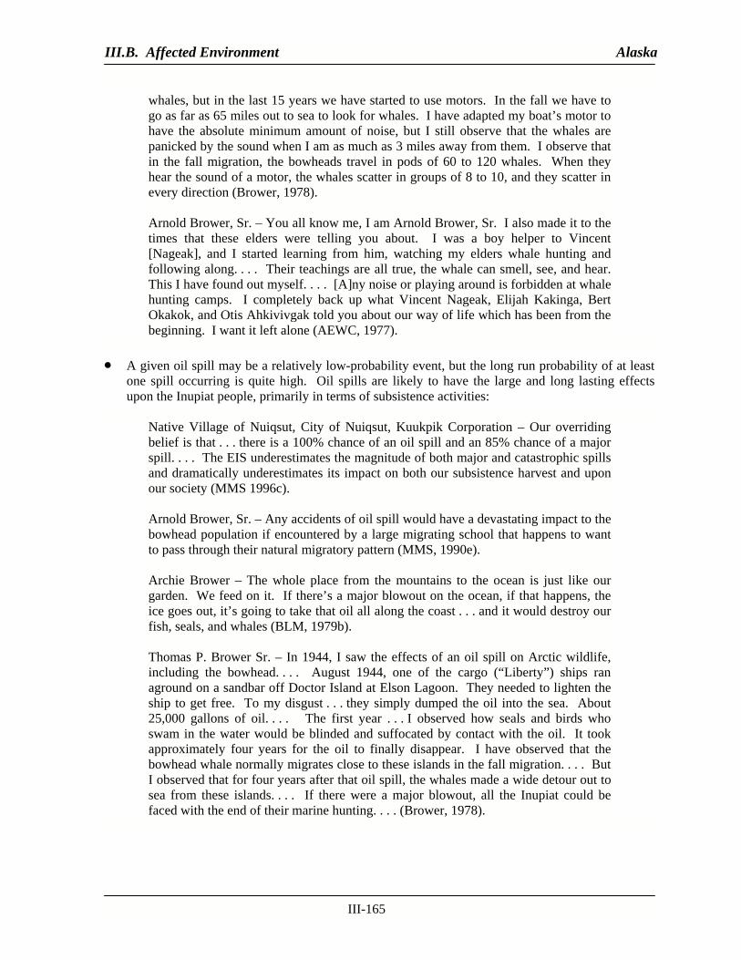
III.B. Affected Environment Alaska
III-165
whales, but in the last 15 years we have started to use motors. In the fall we have to go as far as 65 miles out to sea to look for whales. I have adapted my boat’s motor to have the absolute minimum amount of noise, but I still observe that the whales are panicked by the sound when I am as much as 3 miles away from them. I observe that in the fall migration, the bowheads travel in pods of 60 to 120 whales. When they hear the sound of a motor, the whales scatter in groups of 8 to 10, and they scatter in every direction (Brower, 1978). Arnold Brower, Sr. – You all know me, I am Arnold Brower, Sr. I also made it to the times that these elders were telling you about. I was a boy helper to Vincent [Nageak], and I started learning from him, watching my elders whale hunting and following along. . . . Their teachings are all true, the whale can smell, see, and hear. This I have found out myself. . . . [A]ny noise or playing around is forbidden at whale hunting camps. I completely back up what Vincent Nageak, Elijah Kakinga, Bert Okakok, and Otis Ahkivivgak told you about our way of life which has been from the beginning. I want it left alone (AEWC, 1977).
• A given oil spill may be a relatively low-probability event, but the long run probability of at least
one spill occurring is quite high. Oil spills are likely to have the large and long lasting effects upon the Inupiat people, primarily in terms of subsistence activities:
Native Village of Nuiqsut, City of Nuiqsut, Kuukpik Corporation – Our overriding belief is that . . . there is a 100% chance of an oil spill and an 85% chance of a major spill. . . . The EIS underestimates the magnitude of both major and catastrophic spills and dramatically underestimates its impact on both our subsistence harvest and upon our society (MMS 1996c). Arnold Brower, Sr. – Any accidents of oil spill would have a devastating impact to the bowhead population if encountered by a large migrating school that happens to want to pass through their natural migratory pattern (MMS, 1990e). Archie Brower – The whole place from the mountains to the ocean is just like our garden. We feed on it. If there’s a major blowout on the ocean, if that happens, the ice goes out, it’s going to take that oil all along the coast . . . and it would destroy our fish, seals, and whales (BLM, 1979b).
Thomas P. Brower Sr. – In 1944, I saw the effects of an oil spill on Arctic wildlife, including the bowhead. . . . August 1944, one of the cargo (“Liberty”) ships ran aground on a sandbar off Doctor Island at Elson Lagoon. They needed to lighten the ship to get free. To my disgust . . . they simply dumped the oil into the sea. About 25,000 gallons of oil. . . . The first year . . . I observed how seals and birds who swam in the water would be blinded and suffocated by contact with the oil. It took approximately four years for the oil to finally disappear. I have observed that the bowhead whale normally migrates close to these islands in the fall migration. . . . But I observed that for four years after that oil spill, the whales made a wide detour out to sea from these islands. . . . If there were a major blowout, all the Inupiat could be faced with the end of their marine hunting. . . . (Brower, 1978).

III.B. Affected Environment Alaska
III-166
• Many NSB residents believe that the technology to clean up oil spills in arctic waters, and especially in broken ice conditions, is poorly developed and has not been adequately demonstrated to be effective.
Morgan Solomon – Even if we say to go ahead and develop the land, there is no known technology to protect it if there should be a blowout . . . the oil companies within the Prudhoe area do not have modern equipment to stop any blowout, and they know it (ADNR, 1978).
• One of the most important mitigating measures proposed repeatedly by the NSB, if offshore
drilling must occur, is that no drilling below the threshold where oil is expected to be encountered should take place after April 15.
NSB – While drilling can be conducted year-round above a predetermined threshold depth, it should only be conducted below that depth during the frozen winter months, from November 1 through April 15. Confirmation, extension, and delineation drilling, well testing, and other well completion activities should be concluded by June 15. Finally, all nonessential vessel and air traffic associated with a drilling program should not occur in any particular area during the bowhead whale migration. These policies are reflected in our Land Management Regulations, Section 19.70.040 (NSB, 1991).
• Many NSB residents believe that public comments at public hearings and other public forums may
be noted, but have little or no effect on project decisions or the overall direction and philosophy of the leasing program.
Eben Hopson – Let me again repeat. We have told you why we don’t want the lease sale. We have repeatedly told you why we don’t want the lease sale. We have repeatedly told you for the whole week daily why we don’t want a lease sale. The problem is you don’t want to [?], you don’t want to understand (ADNR, 1978). Joe Nukapigak – Sometimes our testimonies are just being–they’re dissipate once we testify. . . sometimes I feel that my comments are taken for granted, just to be pushed aside. . . . (MMS, 1996c).
Patsy Tukle, through Thomas Nupagiak as translator – He . . . it’s hurt him. . . . Knowing that Inupiat doesn’t have a written law, he hates you guys when you’re coming with big books, tell us what to do. Even against the will of the people who talk, you still go ahead and do it anyway against the will of the people who talk…the will of the Inupiat people. . . . You let us talk; you take our words back to you, and it just doesn’t seem to show in your books that we have spoken (MMS, 1996c).
• There is a general fear of cultural change, especially in terms of the loss of a subsistence lifestyle,
which may lead to social disruptions or social problems in local communities (including youth becoming less interested in traditional ways).
Mark Ahmakak – You wanted some comments on why we are opposing this State lease sale. Reason number one is that this sale is very threatening to our very own lifestyle. Not only to the older people but also to the next generation. Not only on the

III.B. Affected Environment Alaska
III-167
basis of food which we live on which comes from the ocean, the land. . . . (ADNR, 1978).
Edward Nukapigak – And I feel and strongly oppose this Pt. Thompson lease sale because oil companies don’t have enough technology up to this date. Because its gonna really affect our lifestyle in the region of North Slope Alaska. Ever since I was about seven years old, that’s when I started following my dad, how to hunt, how to fish. Might as well [inaudible or trails off] (ADNR, 1978).
• Oil development will result in an influx of population and other influences, which will disrupt and degrade Inupiat community life. In addition, oil development and its effects will impose additional demands upon Inupiat communities and individuals (and appearances at numerous hearings and the review of numerous documents are only the most visible of such demands).
Mark Ahmakak – At this time and age, we’re living in a combination of economic development and uses of the land (for) such (things) as hunting and fishing, subsistence life mixing with our cash economy system. . . . I’d like to see all my kids grow up to be culturally tied to our native culture instead of completely giving in to the cash economy (Kruse et al., 1983b).
Comments reflecting all of these views are well represented in Volume II of the Final EIS for Lease Sale 144 (MMS, 1996c).
(2) Bering Sea Subregion Bristol Bay: The Bristol Bay Region is a culturally diverse area and includes the primary communities of Togiak, Twin Hills, Dillingham, Clarks Point, Ekuk, Naknek, South Naknek, Egegik, Pilot Point, Ugashik, Port Heiden, Port Moller, and Nelson Lagoon. Villages in the Bristol Bay region are predominantly Alaskan Native with the exception of King Salmon, and Iliamna. The cultures represented in this region are solely Yup’ik Eskimo in the Kuskokwim Bay and river areas and a mixture of Yup’ik, Aleut, and Athabascan cultures elsewhere. Within Bristol Bay, Yup’ik people generally inhabit the northern part of the Bay and the interior river systems, while Aleut people generally populate the Alaska Peninsula easterly to Naknek. The central part of the bay contains a mixture of Yup’ik and Aleut people while the inland Iliamna Lake area is inhabited by a mixture of Yup’ik, Aleut, and Athabascan people. Villages in the Togiak subregion (Togiak and Twin Hills) and the Nushagak River villages (Dillingham, Clarks Point, and Ekuk) are based on traditional Yup’ik cultures; the Upper and Lower Alaska Peninsula communities (Naknek, South Naknek, Egegik, Pilot Point, Ugashik, Port Heiden, Port Moller, and Nelson Lagoon) are based in traditional Aleut culture blended with Russian and Scandinavian influences (BLM, 1982e; Wolfe et al., 1984; MMS, 1985b, 1985c, 1985d, 1991b, 1991c). The most important values found throughout the region are those associated with the ideology of subsistence and commercial fishing as a means of livelihood; and, although distinct cultural differences abound within the region, the principal similarity among people is the occupational identification of fishermen, and the profound similarities are the role of kinship in organizing work, leisure, household formation, and ritual activity. The extended family has tended to give way to the nuclear family since the 1960’s. The meaning of subsistence practices and activities culturally is to perpetuate and celebrate the local community as a socially value laden phenomenon among families, generational groups, and a wider group of people of similar value orientation (BLM, 1982e; MMS,

III.B. Affected Environment Alaska
III-168
1985b, 1985c, 1991b, 1991c). However, with the declines in some of the fisheries and attendant changes in local economics and demographics, some communities are examining strategies to ensure their viability and stability. Aleutians: The primary communities of the Aleutians region are Akutan, Unalaska, Dutch Harbor, Nikolski, Atka, and Adak. Aleutians sociocultural systems distinctly follow the traditions of the Aleut. Hunting, fishing, and gathering continue to be crucial to their cultural experience. Family patterns, sex and age roles, community organization, leadership, and social life still continue to be influenced by subsistence requirements and the resources of the maritime environment. Although there are differences in the cultural traditions of the Aleuts region, kinship forms the basis of their social organization and cultural values, and orientations continue to lean towards their Aleut subsistence heritage (MMS, 1983, 1985c, 1985d, 1991b, 1991c). Within the region, Unalaska and Dutch Harbor are the communities most likely to be affected by oil development. These communities are divided between the traditional Aleut community in Unalaska and seafood processing in the Dutch Harbor area with a culturally diverse community populated by a majority of transient fishermen and laborers. Cultural values and orientations vary according to the social group, ranging from traditional Native values in Unalaska to values of the larger American culture more common in Dutch Harbor (MMS, 1983, 1985a, 1985b, 1985c, 1991a, 1991b).
(3) South Alaska Subregion Kodiak: The City of Kodiak is the largest and most culturally diverse community on Kodiak Island. The City of Kodiak and its surrounding road-connected residential areas provide diversified social, commercial, and other services for residents of Kodiak Island, in addition to an important commercial-fishing port. The single most unifying aspect among sociocultural groups in Kodiak is the fishing industry. This economic mainstay of the community permeates the entire social fabric of the community. Kodiak is the home of the largest commercial-fishing fleet in Alaska (Fall et al., 2001; MMS, 1984b). The isolation and relatively small size of the Kodiak area encourage rapid organization and mobilization around key issues affecting the community. Issues that could affect the fishers way of life have tended to generate considerable unity (Fall et al., 2001; Impact Assessment, Inc., 2001; MMS, 1984b). The nonroad-connected communities on Kodiak Island are much smaller and culturally homogeneous. These settlements, Akhiok, Karluk, Larsen Bay, Old Harbor, Ouzinkie, and Port Lions, are primarily Alutiiq villages. Each represents small systems of extended families that are subsistence- and family-oriented, and predominantly Russian Orthodox, in keeping with a long history of Alutiiq-Russian contact (MMS, 1984b, 2003b). Kodiak Island communities are incorporated into the KIB, formed in 1963 as a second-class borough. The KIB also includes uninhabited coastal lands opposite the archipelago on Shelikof Strait. The City of Kodiak is a home-rule city, formed in 1940; five of the nonroad-connected communities (except Karluk) incorporated as second-class cities in the late 1960’s and mid-1970’s. Tribal councils also exist in these communities. The Karluk Tribal Council was formed in 1939 and is recognized by the State of Alaska as the local community government (Cultural Dynamics, Ltd., 1986a). The Kodiak Area Native Association provides regional tribal services to most of the Native communities. Koniag, Inc. is the regional ASCSA corporation for the communities on Kodiak Island (MMS, 2003b). A strong pattern of involvement and diversification in fisheries is found in the communities of Old Harbor, Port Lions, and Ouzinkie, although traditional fishers are also present. Port Lions appears to be most similar to the City of Kodiak in the size of vessels, the fisheries pursued, and the proportion of total earnings derived from different species (MMS, 2003b).

III.B. Affected Environment Alaska
III-169
Other communities show a pattern of declining involvement in commercial fisheries, a pattern found in Larsen Bay, Akhiok, and Karluk—originally traditional salmon-oriented communities. Fishers from these communities have sold most of their permits, particularly set-gillnet permits, for a variety of reasons, such as poor local harbors, lack of vessel- and gear-storage facilities, natural disasters, and poverty. Although commercial fishing is still important in Larsen Bay, participation is declining. Residents of Akhiok and Karluk appear to be only minimally involved in commercial fisheries (MMS, 2003b). Cook Inlet: This subregion is quite diverse. Anchorage is the largest urban community in the State and its major service center. Most of the area is connected to Anchorage by road, and Anchorage is also the center of scheduled and charter aircraft (MMS 1992, 2003b). The communities of the upper Cook Inlet and Kenai Peninsula are organized under the KPB, a second-class borough incorporated in 1964. The KPB includes most of the Kenai Peninsula and coastal lands on the west side of Cook Inlet. Seldovia incorporated as a first-class city in 1945, and Kenai as a home-rule city in 1960. Homer and Soldotna incorporated as first-class cities in the mid-1960’s. Tyonek organized a tribal council under the Indian Reorganization Act in the late 1930’s; it remains the governing body for the community (Fall et al., 1984). Regional tribal organizations include the Cook Inlet Tribal Council and Chugachmiut. Regional Alaska Native Claim Settlement Act corporations include Cook Inlet Region Inc. and Chugach Alaska Corporation (MMS, 2003b). Fishing, tourism, oil and gas, and government support the Kenai Peninsula’s diversified economic, social, and commercial activities. Tourism and recreation is an important and growing sector, and sport fishing remains the largest single attraction on the Peninsula. The Kenai River flows through the area and supports the largest sport fishery in Alaska. Since the late 1950s, the social fabric and economy of the Kenai-Soldotna area have been shaped most by the development of oil and gas resources on the Kenai Peninsula and in Cook Inlet. The local petroleum industry spawned associated industries such as refining and chemical manufacturing and has provided important services to North Slope oil fields. The sociocultural systems of these large coastal communities are supported by this diversified economic base with sizeable growth through inmigration. The Kenai-Soldotna area (i.e., Kenai, Soldotna, Nikiski, Sterling, Ridgeway, Salamatof, and Kasilof) serves as a diversified service center for the central Kenai Peninsula area. The Homer area serves as a smaller scale hub for the southern Kenai Peninsula. This area encompasses the City of Homer and the residential areas of Fritz Creek, Anchor Point, Nikolaevski, Ninilchik, and Kachemak (S.R. Braund & Associates, 1980; Georgette, 1983; MMS, 1984b, 2003b). Small communities located in Cook Inlet that are not connected to the road network include Tyonek, Nanwalek, Port Graham, and Seldovia. Residents of Tyonek are predominantly Tanaina (Dena’ina) Athabaskan Indians; residents of Nanwalek and Port Graham are predominantly Alutiiq people who locally refer to themselves as Aleuts. The relative isolation of Port Graham and Nanwalek has allowed these communities to maintain their Alutiiq identity and traditions with limited external interference. All of these communities but Seldovia are predominantly Native with limited commercial economic opportunities, primarily related to fishing and fish processing. Seldovia and Ninilchik have deep historical roots in the region and have undergone considerable social and cultural change. Seldovia is a multi-ethnic community with a character similar to other rural, white, frontier fishing towns. It has a relatively heterogeneous population and Alaska Native populations of Athabascan and Alutiiq heritage. Seldovia in the early 1900’s was a thriving commercial-fishing community and the center for commercial and social life for all of Kachemak Bay and Cook Inlet. Many Scandinavian and other fishermen immigrated there and intermarried with the local population.

III.B. Affected Environment Alaska
III-170
In the 1960’s, other commercial centers outgrew Seldovia and diminished its commercial importance. Seldovia today has a sizeable, yet declining, Alaskan Native population. Ninilchik, a previously isolated Russian Orthodox fishing village, now has many residents with nonlocal employment such as on Cook Inlet offshore platforms. New residents have brought a wide range of values, beliefs, skills, and cultural traditions, but this community still retains a sizable core of lifelong Ninilchik families engaged in commercial fishing (Braund and Behnke, 1980; Reed, 1983; MMS, 1984b, 2003b). Subsistence is characterized by a well-established annual round of hunting, fishing, and gathering activities; the use of a wide range of marine and land resources; and a kinship-based system for the harvest, processing, distribution, and exchange of wild-resource products. Subsistence activities are important and reinforce the fundamental kinship-based social organization of these communities (Braund and Behnke, 1980; S.R. Braund & Associates, 1980; (Fall, 1983; Reed, 1983; Schroeder et al., 1987a; Fried and Windisch-Cole, 1999; MMS, 2003b).
b. Subsistence The term “subsistence” has different definitions and meanings (Davidson, 1974; Arnold, 1978; Lewis, 1978; Lonner, 1980; Kelso, 1981, 1982; Case, 1984, 1989; Berger, 1985; Caulfield and Brelsford, 1991; Bryner, 1995; Naiman, 1996; ADNR, 1997; Loescher, 1999). The ANILCA provides the basis for the definition of the term subsistence in this document. Other legislative acts and regulatory actions relevant for the understanding of subsistence management issues on Federal lands include the Federal Subsistence Management Regulations (36 CFR 242 or 50 CFR 100 as summarized and available in FWS [1999b]), the Federal Advisory Committee Act, and the Federal Advisory Committee Management Regulations (41 CFR 101-6). The MMPA and ESA are also pertinent, addressing the harvest of marine mammals currently restricted to subsistence use by coastal Natives. The ANILCA explicitly recognizes that for rural Alaskans (Native and non-Native), “subsistence” subsumes a complex set of behaviors and values that extend far beyond the harvest and consumption of wild resources, although it is formally defined primarily in those terms. The current regulations define “subsistence use” as
. . . the customary and traditional uses by rural Alaska residents of wild, renewable resources for direct personal or family consumption as food, shelter, fuel, clothing, tools of transportation; for the making and selling of handicraft articles out of nonedible by-products of fish and wildlife resources taken for personal or family consumption; for barter, or sharing for personal or family consumption; and for customary trade (FWS, 1999b).
Customary and traditional use of a specific subsistence resource is evaluated in terms of several factors: • • • • •
• •
time, depth, and consistency of its use; seasonal repetition of such use over many years; efficiency in terms of effort and cost of such use; consistency of the harvest or use of fish and wildlife in proximity to the community or area; historic or traditional means of handling, preparing, preserving, and storing fish and wildlife that have been used by past generations; intergenerational transmission of hunting and fishing skills, values, and knowledge; the sharing and distribution of the harvest;

III.B. Affected Environment Alaska
III-171
• •
dependency upon a wide variety of fish and wildlife resources available in an area; and the provision of substantial cultural, economic, social, and nutritional elements to the community or area.
“Subsistence” as a label thus incorporates a complex set of behaviors and values that extends far beyond the harvesting and consumption of wild resources. Fundamental values are expressed in subsistence, so that kinship, sharing, and subsistence resource use behaviors (i.e., preparation, harvest, processing, consumption, and celebration) become inseparable (Langdon and Worl, 1981; Elanna and Sherrod, 1984). Worl (1979) and Nelson (1979) describe subsistence as a central focus of North Slope personal and group cultural identity in addition to its economic role. Hopson (1976, 1978) establishes the political and ideological power of subsistence as an organizing concept for the NSB. Simeone (1998) documents its central place in village life and identity in Athabaskan communities. McNeary (1978) and North Pacific Rim (1981) describe the socioeconomic aspects of subsistence in the changing cultural landscape of the Prince William Sound region. In each region, communities express their unique identities through enduring connections between current residents, past residents, and the wild resources of the land. Elder’s conferences, spirit camps, and other events serve to solidify the cultural connections between generations, and between the people and the land and its resources. Many studies have examined the relationship between subsistence and wage economies and how both subsistence and wage activities are integrated into rural Alaskan socioeconomic systems (Wolfe 1983; Wolfe et al. 1984; Impact Assessment, Inc. 1988). Although not always made explicit, it is recognized that all rural communities and rural socioeconomic systems are not the same. One salient variable is the ethnic composition of the community; another is the diversification of the local economy and the availability of wage employment. An extensive study series across a wide range of Alaskan communities focused on local patterns of wild resource use as a component of the overall economy (Galginaitis et al., 1984; Reed, 1985; Sobelman, 1985; Impact Assessment, Inc., 1989; Stratton, 1989, 1990, 1992; Fall and Utermohle 1999). Some communities are predominantly Native, while others are predominantly non-Native, and others more ethnically “mixed.” Some have developed wage economies; others have few such opportunities. Within the NSB, both subsistence activities and wage economic opportunities are highly developed and highly dependent upon each other (Kruse et al., 1981; Kruse, 1982, 1991; Harcharek, 1995; Shepro and Maas, 1999). Those communities most active in subsistence activities tend to be those who are also very involved in the wage economy. That is, monetary resources are needed to most effectively harvest subsistence resources. Native subsistence users as a group display a different pattern of resource harvests, consumption, and sharing than do non-Natives (Impact Assessment, Inc. 1988; Human Relations Area Files 1994a,b, c). Subsistence foods consist of a wide range of fish and game products and are generally rich in nutrients and low in fats, and they contain more heart-healthy fats and less harmful fats than many non-Native foods (Nobmann, 1997). Social, emotional, spiritual, and cultural benefits are other important aspects of subsistence food harvesting and sharing that contribute to personal and community health. Rural Alaskans harvest more than 40 million pounds of wild foodstuffs every year (Wolfe, 1996). On average, food produced through hunting, fishing, and gathering amounts to just over 1 pound of wild food per person per day. Actual consumption may vary from what is harvested or brought into the kitchen. However, few wild food consumption studies have been undertaken in Alaska. Broad regional discussions of selected aspects of subsistence resource harvest activities are provided below. Summary descriptive information for most regions and many communities within those regions is available (Schroeder et al., 1987a; ADF&G, 2004a).
III.B. Affected Environment Alaska
III-172
(1) Arctic Subregion In the Beaufort and Chukchi Sea regions, North Slope subsistence resource harvest activities have been relatively well documented, and the following discussions incorporate this information by reference (BLM, 1978a, b; 1979a, b, c, d; 1982a, b, c, d, e; 1983a, b; 1990, 2003; MMS, 1984a; 1986; 1987a, b; 1990c, d, e; 1991b, 1996a, c; 1997; 1998b; 2001a; 2003a; S.R. Braund & Associates, 1988; ADNR, 1997, 1998, 1999a; BLM and MMS, 1998; COE, 1999). These sources contain regional overviews as well as discussions of relevant communities, and present of more detailed information as required for the purposes of specific planning documents. Each is also supported by an extensive record of public hearing testimony and written comments. Each North Slope community exhibits a unique pattern of subsistence resource use, but caribou are harvested by residents of all North Slope communities and are the most important terrestrial subsistence resource. Fish are also harvested by residents of all villages and are a primary resource for all except Anaktuvuk Pass, an inland community with limited access to fish. Kaktovik, Nuiqsut, Barrow, Wainwright, Point Lay, and Point Hope rely heavily upon and harvest three animal resource categories–whales and other marine mammals, caribou, and fish. Anaktuvuk Pass relies primarily upon caribou, but receives a good amount of fish and whale through sharing and other modes of exchange. Residents of Anaktuvuk Pass and Atqasuk also receive whale through their participation as members of whaling crews in other communities (Hoffman et al., 1988; Shapiro et al., 1979; North Slope Borough Contract Staff, 1979; Jacobson and Wentworth, 1982; Nelson, 1982; Braund and Burnham, 1984; Schneider et al., 1980; George and Nageak, 1986; George and Kovalsky, 1986; Luton, 1986; Alaska Consultants, Inc. et al., 1984; Craig, 1987; S.R. Braund & Associates, 1989a, b; Impact Assessment, 1990a, b; S.R. Braund & Associates and UAA, ISER, 1993a, b; Lowenstein, 1994; Suydam et al., 1994; Stephensen et al., 1994; Harcharek, 1995; Brower and Opie, 1997; Moulton, 1997; Brower and Hepa, 1998; NSB, 1998; BLM, 1998; Burch, 1998; Fuller and George, 1997; Brower et al., 2000; Kassam and Wainwright Traditional Council, 2001; BLM and MMS, 2003; MMS, 2002e, 2003a, 2004a; ADF&G, 2004a; BLM, 2004).
(2) Bering Sea Subregion Bristol Bay: Most Native Alaskans of the Bristol Bay region are involved in summer commercial salmon fishing in some form or another. For many, this is the primary source of cash income for the year, except for those residents living in the larger communities of Dillingham, Bethel, and Naknek, where other employment may be available during the year. Commercial-fishing income is viewed by most of the smaller communities largely as a means of subsidizing subsistence pursuits during the remainder of the year. This subsistence orientation is repeatedly demonstrated year after year in the large subsistence salmon harvest (BLM, 1982e). In the Bristol Bay region as a whole, salmon, caribou, and moose are the more important subsistence resources to almost all of the villages in the region. Caribou is most highly used per household in the Iliamna and Upper and Lower Alaska Peninsula subregions. Sea mammals, migratory birds and waterfowl, and beaver for fur also are harvested when available throughout the year. Nelson Island has a local herring fishery. Local harvesting of caribou increased slightly in the early 1980’s due to better access with all-terrain vehicles (Earl. R. Combs, Inc., 1981; BLM, 1982e; MMS, 1985b, 1985c, 1985d, 1991b, 1991c; Coiley-Kenner et al., 2003). For communities in the northern Bristol Bay region, the average annual wild-food harvest ranged from 242 pounds per person in Dillingham to 363 pounds per person in Clarks Point. Most of the subsistence wild food is composed of fish (58% by weight) along with land mammals (34%, primarily moose and caribou) and marine mammals (2%). In addition, shellfish, birds and eggs, and plants

III.B. Affected Environment Alaska
III-173
make up another 4 percent of the harvest by weight. Salmon harvests provide a large portion of the region’s wild food each year (47%). Of the five species of salmon harvested, sockeye salmon is the most prominent. From 1985-1999, the annual subsistence harvests of sockeye salmon ranged from 22,461 to 49,225 fish (http://www.commerce.state.ak.us/dca/AEIS/AEISMainFrame.cfm? CensusArea=Dillingham&Industry=Subsistence&IndexItem=SubsistenceOverview). In the central Bristol Bay region, the average annual wild-food harvest ranged from 188 pounds per person in Naknek to 297 pounds per person in South Naknek. Most of the subsistence wild food is composed of fish (55% by weight) along with land mammals (37%, primarily caribou) and marine mammals, shellfish, birds and eggs, and plants making up another 8 percent of the harvest by weight. Salmon harvests provide a large portion of the region’s wild food each year (47%). Of the five species of salmon harvested, sockeye salmon is the most prominent. From 1985-1999, the annual subsistence harvests of sockeye salmon ranged from 11,275 to 23,573 fish (http://www.commerce.state.ak.us/dca/ AEIS/AEISMainFrame.cfm?CensusArea=Bristol&Industry=Subsistence&IndexItem=SubsistenceOverview). In Upper Alaska Peninsula communities fronting the Bristol Bay coast, the average annual wild-food harvest ranged from 257 pounds per person in Nelson Lagoon to 814 pounds per person in Ugashik. Most of the subsistence wild food is composed of fish (58% by weight) along with land mammals (33%; primarily caribou) and marine mammals (3%). Shellfish, birds and eggs, and plants making up another 6 percent of the harvest by weight. Salmon harvests provide a large portion of the region’s wild food each year (48%). Of the four species of salmon harvested, sockeye salmon is the most prominent. From 1985-1999, the annual subsistence harvests of sockeye salmon ranged from 62,877 to 110,335 fish (http://www.commerce.state.ak.us/dca/AEIS/AEISMainFrame.cfm?CensusArea= LakePen&Industry=Subsistence&IndexItem=SubsistenceOverview; http://www.commerce.state.ak.us/ dca/AEIS/AEISMainFrame.cfm?CensusArea=AleutEast&Industry=Subsistence&IndexItem=SubsistenceOverview; see also, Morris, 1982, 1985; Wolfe et al., 1983, 1986; Wright and Chythlook, 1985; Wright et al., 1985; Fall and Morris, 1987; MMS, 1996a; Seitz, 1990, 1996; Fall et al., 1986, 1990, 1991, 1996, 1997; Gross, 1991; Kreig,et al., 1996; Kreig et al., 1998; Wolfe and Mishler, 1993, 1994, 1995, 1998; Wolfe and Hutchinson-Scarbrough, 1999; Wolfe, 2001; Wolfe et al., 2002). Regional Traditional Knowledge on Subsistence: Below are several examples of testimony given by residents in the Bering Sea Subregion on the subject of subsistence.
In hearings for the Alaska Native Claims Settlement Act, Yup’ik Elder Paul John from the Native community of Tununak spoke this way about the Yup’ik subsistence lifestyle—Our subsistence way of life is especially important to us. Among other needs, it is our greatest. We are desperate to keep it (Fienup-Riordan, 1986).
Ulric Nayaman, a former member of the Chevak Traditional Council and a respected elder of the region explained the problematic relationship Yup’ik people have with modern technology – To simply broaden your vision of our lifestyle: The oil we use is not produced by our community but we need it. If, however, a spill does occur, it will touch our stomachs. We aren’t like you. If we have troubles, we can’t turn to a bank. The coast is our bank… (Fienup-Riordan, 1986). A St. Paul subsistence hunter spoke about the community’s relation to the fur seal this way – In the early days, my grandpa or somebody would say, ‘The seal is our brother, He lives on the island and you live off of him, so you treat him like a brother.’ So we live by tradition (ADF&G, 1996).

III.B. Affected Environment Alaska
III-174
A Yup’ik subsistence hunter from the Bristol Bay community of Togiak recounted the regional subsistence preference for seal and sea lion – Please don’t close this subsistence way of life for hunting seals and sea lions, even all wildlife because it’s our heritage, our culture, our way of life. Our old people have a saying that if people stopped eating seals and sea lions, it will change our way of life, our lives, the way we eat. It will even affect our flesh (ADF&G, 1996). A subsistence hunter from Unalaska explained local subsistence practices in the community – There are still community hunters going out and bringing back resources for the people. And when the salmon start running, people bring it back. The rule in Native villages is you always got to eat and there is always somebody out there to get something. Of course, you take care of the older people first. We always give them first choice (ADF&G, 1996).
(3) South Alaska Subregion Kodiak: For the Island of Kodiak, the smaller and predominantly Native villages have similar patterns of subsistence resource use, and differ significantly from that of the City of Kodiak, which is much larger, more ethnically diverse, but with a much smaller percentage of Native population. Native subsistence communities on Kodiak Island have a maritime cultural tradition and are dependent on the seas. Their pattern of subsistence use consists of fishing for salmon, halibut, and other fish in summer; hunting and gathering sea mammals, shellfish, and intertidal resources in winter and spring; hunting deer, ducks, rabbits, and ptarmigan to provide major protein sources in winter; and summer berry picking. The principal wild foods harvested by the local Native communities of Akhiok, Karluk, Larsen Bay, Old Harbor, Ouzinkie, and Port Lions in the Kodiak Island Borough are fish (71% of the total annual harvest, land mammals (14%), and shellfish (6%). Salmon consistently provide the major portion (52%) of the region’s subsistence food, and sockeye is the most harvested. From 1985-1999, the annual average harvest for the region ranged from 16,177 fish to 43,737 fish. Marine mammals make up 4 percent, plants 3 percent, and birds and eggs 2 percent of the total annual harvest. Other major fish harvested are halibut, Pacific cod, Dolly Varden, and sablefish. Important land mammals taken are Sitka deer, moose, elk, and hare. Preferred marine mammals are Steller sea lion and harbor seal. Primary shellfish varieties consist of tanner crab, Dungeness crab, and butter clams (http://www.dced.state.ak.us/dca/AEIS/AEISMainFrame.cfm?CensusArea=Kodiak&Industry=Subsistence&IndexItem=SubsistenceOverview; MMS, 1995a). Cook Inlet: A picture of subsistence in this region is complex for a variety of reasons. The region includes the city of Anchorage, an urban area with 42 percent of the State’s population. Anchorage is “nonrural,” but its residents hunt and fish under “sport” regulations, especially in the Kenai Peninsula. Also, until recently, parts of the Kenai Peninsula itself were considered “nonrural,” and data on subsistence resource use by the residents of many communities are lacking. Most of this area is connected by a road network, and most communities are of mixed ethnicity or predominantly non-Native. Four predominantly Native communities are not on the road network: Seldovia is on Seldovia Bay; Port Graham and Nanwalek are on bays west of Seldovia Bay; and Tyonek is on the west coast of Cook Inlet. These predominantly Native villages share many of the same characteristics of communities in the less economically developed parts of the State. Economic opportunities are limited (other than commercial fishing), and subsistence resources are important to the household economy in terms of variety, amount, and sharing. Road-connected communities of the region display

III.B. Affected Environment Alaska
III-175
somewhat different patterns of subsistence resource use (Georgette, 1983; C.E. Reed, 1983, 1985; ADF&G, 1999a, b; ADNR, 1999b; Borass, 2002). Subsistence activities are assigned the highest cultural values by local Cook Inlet Dena’ina, Kenaitze, Alutiiq, and Koniag Native harvesters, providing a sense of identity as well as an important economic pursuit. Since many species play an important role in the annual cycle of subsistence-resource harvests, effects on subsistence can be serious even if the net quantity of available food does not decline. Beyond dietary benefits, subsistence resources provide materials for personal and family use, and the sharing of resources helps maintain traditional family organization. Subsistence use patterns vary considerably in the Cook Inlet region. Smaller, more traditional villages harvest salt and freshwater fish and small sea mammals in summer and fall, hunt moose in the fall, and harvest invertebrates and some sea mammals all year. Residents in the more urban-based communities fish in the summer and hunt in the fall. While the Kenaitze, a group of Dena’ina Athabascans, have used Cook Inlet natural resources for generations, the ADF&G did not allow a Kenaitze Tribal Fishery until 1989. Fishing dates vary from year to year; in 1995 it was conducted from May 1 to October 15. Fishing occurs primarily in coastal marine waters south of the mouth of the Kenai River and occasionally immediately upstream of the Warren Ames Bridge in Kenai. The tribal office reported a 1997 harvest of 142 chinook, 2,410 sockeye, 5 pink, and 191 coho salmon (ADNR, 1999b). Residents of Ninilchik and members of the Kenaitze Tribe harvest fish resources (primarily salmon) on the east side of Cook Inlet. Other major resources are halibut and butter/razor clams. Established in 1993, the Ninilchik Traditional Council Fishery allows a local subsistence salmon harvest. Fishing time varies but is normally held May 8-September 30. The harvest totals for the 1997 season were 302 chinook, 241 sockeye, 99 coho, and 55 pink salmon (most recent harvest data). Ninilchik residents harvest moose in the fall after the fishing season (ADNR, 1999b). Nanwalek and Port Graham residents harvest and use a wide range of subsistence resources and maintain considerable networks of resource sharing and distribution. These two villages are closely related by family ties, common hunting and fishing practices, and local custom (MMS, 1992). Residents of Seldovia, Port Graham, and Nanwalek are the primary subsistence harvesters of the lower Kenai Peninsula, and, since the Exxon Valdez oil spill fouled local traditional clamming areas, residents of Nanwalek and Port Graham have used the area around Ninilchik for the harvest of razor clams. Subsistence harvesting of fish, wildlife, and vegetation also occurs at the head and along the southern shore of Kachemak Bay. Area residents harvest seals, sea lions, and sea otters around Yukon Island and Tutka Bay. Primary waterfowl harvest areas are in the vicinity of Seldovia, Tutka, and China Poot Bays and McKeon and Fox River flats. Seabirds and their eggs also are harvested. Moose, black bear, and mountain goats are hunted along local shorelines. Port Graham and Nanwalek residents harvest salmon in Nanwalek and Koyuktolik (“Dogfish”) Bays. Seldovians gather berries in larger quantities than any of the other Kenai Peninsula subsistence communities (ADNR, 1999b). Resources preferred by Nanwalek and Port Graham residents are clams, moose, bear, and especially salmon. These provide large quantities of food during a short period of the year and also are preserved for use throughout the remainder of the year. A combination of commercial, subsistence, and rod-and-reel fisheries provide salmon for domestic use. Residents of Nanwalek and Port Graham participate in permitted general subsistence and personal-use fisheries that have existed in upper Cook Inlet since 1991, open to Natives and non-Natives. Dipnet fisheries take place on the Kenai and Kasilof Rivers and on Fish Creek. A set gillnet fishery takes place on the Kasilof River from June 21 until closed. In

III.B. Affected Environment Alaska
III-176
addition, a general Kachemak Bay subsistence and personal-use salmon fishery has taken place since before Statehood. This fishery uses Fox River drainage salmon runs returning and hatchery stocks returning to the fishing lagoon on Homer Spit and to Fox Creek. In 1993, 326 permits were issued, and 1,990 coho, 463 pink, 44 sockeye, 18 chum, and 6 Chinook salmon were harvested (ADNR, 1999b). Other resources such as trout, cod, halibut, chitons, snails, and crabs are used fresh in season. Harbor seals and sea lions are highly valued marine mammals, are harvested year-round, and are extensively shared within the community. A variety of plants also are harvested in Kachemak Bay. Bull kelp, rockweed, and brown seaweeds are collected from intertidal areas, and shoreline areas provide seaside plantain, rye grass, beach pea, wild parsley, and cow parsnip. Seldovia, Kasitsna, and Jakolof Bays are important areas for the harvest of marine invertebrates. Often overlooked, gardening has been part of village subsistence life since Russian times. Potatoes, cabbage, and turnips were brought to the Kenai Peninsula by Russian settlers who planted gardens out of the need for fresh vegetables (Fall, 1981). A variety of local wild berries are picked, particularly low- and high-bush cranberries, rosehips, blueberries, moss berries, and wild raspberries. Locally harvested subsistence foods are distributed widely among community households. Tyonek, on the west side of Cook Inlet, has a subsistence harvest area that extends from the Susitna River south to Tuxedni Bay; harvests concentrate in areas west and south of Tyonek. Moose and salmon are the most important subsistence resources, although important components of the harvest include nonsalmon fish such as smelt, waterfowl, and clams, as well as a traditionally important beluga whale hunt (ADNR, 1999b). The subsistence use of beluga in Cook Inlet is a sensitive issue. Until recently, this was a relatively undocumented hunt. Recent declines in their population have led Cook Inlet beluga whales to be classified as “depleted.” Due to co-management agreements between NMFS and the Cook Inlet Marine Mammal Council representing Native subsistence hunters, this species has not been formally listed as threatened or endangered. However, while previous harvests were conducted by Natives living in or visiting Anchorage and residents of Tyonek, the current co-management agreement allows only for the harvest of one beluga by the Tyonek community. Regional Traditional Knowledge on Subsistence: Below are several examples of testimony given by Alaskan residents on the subject of subsistence.
Julie Knagin, from Kodiak – The bottom line is that I see that nothing goes to waste. When the Natives catch anything—whether it’s fish, marine mammal--nothing goes to waste. Everything is used. It’s nothing like all those trophies you see in airports all over. . . . That’s our life style. It’s our survival. We never depended on Safeway. We never could. It was never there. We got the basics—coffee, tea, sugar—but everything else was from land and sea and air (Alaska Native Science Commission and UAA, ISER, 2000). Karluk hunter – We’ll never get away from seal. We need it. Young people are learning how to cut them up. Everybody goes down and watches them cut them up. Hunters cut them up. Or, if the hunter didn’t cut them up, get someone experienced. Women do the braiding and cooking (ADF&G, 1999). Larsen Bay subsistence hunter (reflecting on the cultural importance of the subsistence hunts for seal and deer) – Everything is eaten. When we get it, we split it
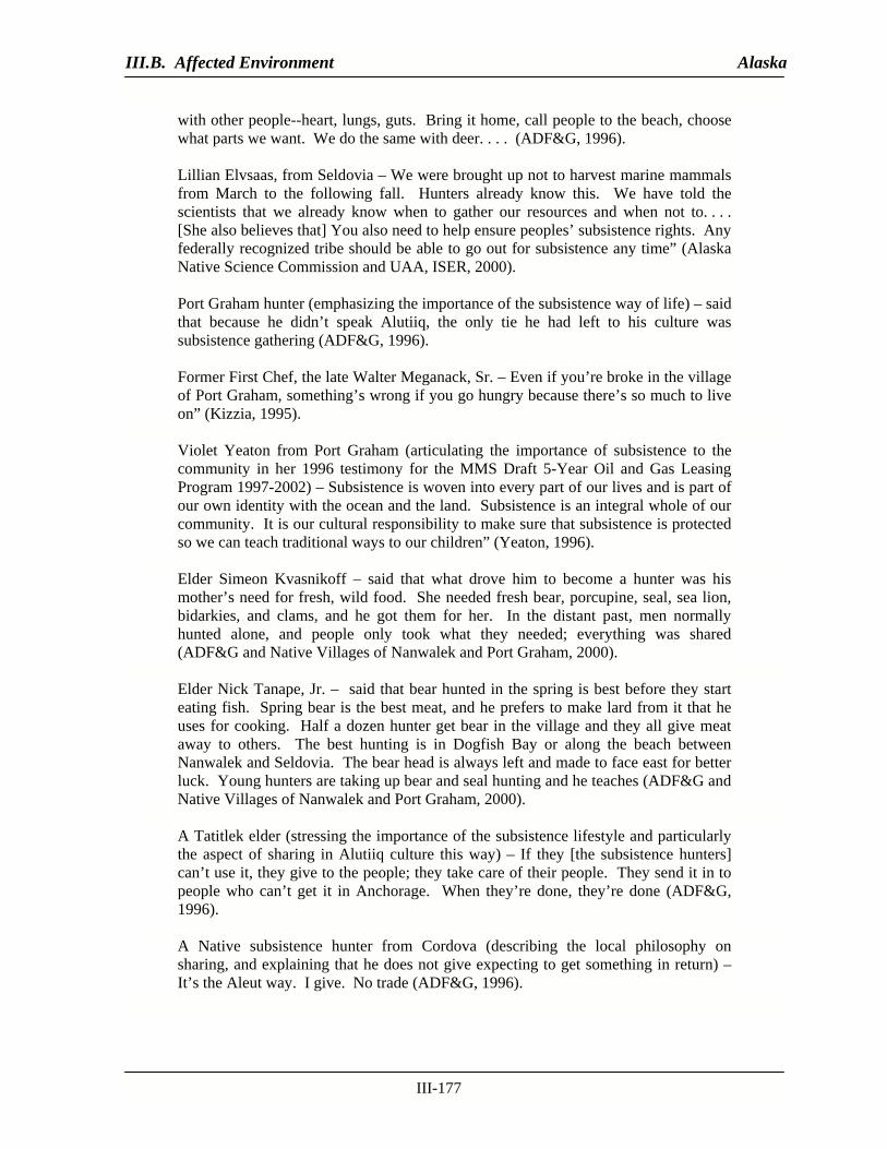
III.B. Affected Environment Alaska
III-177
with other people--heart, lungs, guts. Bring it home, call people to the beach, choose what parts we want. We do the same with deer. . . . (ADF&G, 1996). Lillian Elvsaas, from Seldovia – We were brought up not to harvest marine mammals from March to the following fall. Hunters already know this. We have told the scientists that we already know when to gather our resources and when not to. . . . [She also believes that] You also need to help ensure peoples’ subsistence rights. Any federally recognized tribe should be able to go out for subsistence any time” (Alaska Native Science Commission and UAA, ISER, 2000). Port Graham hunter (emphasizing the importance of the subsistence way of life) – said that because he didn’t speak Alutiiq, the only tie he had left to his culture was subsistence gathering (ADF&G, 1996). Former First Chef, the late Walter Meganack, Sr. – Even if you’re broke in the village of Port Graham, something’s wrong if you go hungry because there’s so much to live on” (Kizzia, 1995).
Violet Yeaton from Port Graham (articulating the importance of subsistence to the community in her 1996 testimony for the MMS Draft 5-Year Oil and Gas Leasing Program 1997-2002) – Subsistence is woven into every part of our lives and is part of our own identity with the ocean and the land. Subsistence is an integral whole of our community. It is our cultural responsibility to make sure that subsistence is protected so we can teach traditional ways to our children” (Yeaton, 1996).
Elder Simeon Kvasnikoff – said that what drove him to become a hunter was his mother’s need for fresh, wild food. She needed fresh bear, porcupine, seal, sea lion, bidarkies, and clams, and he got them for her. In the distant past, men normally hunted alone, and people only took what they needed; everything was shared (ADF&G and Native Villages of Nanwalek and Port Graham, 2000).
Elder Nick Tanape, Jr. – said that bear hunted in the spring is best before they start eating fish. Spring bear is the best meat, and he prefers to make lard from it that he uses for cooking. Half a dozen hunter get bear in the village and they all give meat away to others. The best hunting is in Dogfish Bay or along the beach between Nanwalek and Seldovia. The bear head is always left and made to face east for better luck. Young hunters are taking up bear and seal hunting and he teaches (ADF&G and Native Villages of Nanwalek and Port Graham, 2000).
A Tatitlek elder (stressing the importance of the subsistence lifestyle and particularly the aspect of sharing in Alutiiq culture this way) – If they [the subsistence hunters] can’t use it, they give to the people; they take care of their people. They send it in to people who can’t get it in Anchorage. When they’re done, they’re done (ADF&G, 1996).
A Native subsistence hunter from Cordova (describing the local philosophy on sharing, and explaining that he does not give expecting to get something in return) – It’s the Aleut way. I give. No trade (ADF&G, 1996).

III.B. Affected Environment Alaska
III-178
A Tlingit hunter from Yakutat (reflecting on the importance of marine mammals to the local subsistence harvest and regulatory constraints that can frustrate the harvest) – The idea of using this resource for subsistence, which we are used to, and is protected by the MMPA [Marine Mammal Protection Act] is good. . . . We need it. If you don’t have it, it changes your personality. I have seen this, even myself. I know when I run out, I will walk the streets with dry fish, begging for trade. That’s how much I crave it (ADF&G, 1996).
Another Tlingit hunter from Yakutat (concerning the necessity of the seal subsistence hunt) – We need it. If we don’t have it, it changes your personality (ADF&G, 1996).
c. Climate Change (1) Arctic Subregion In the Arctic Subregion, a factor of increasing concern is the potential for adverse effects on subsistence-harvest patterns and subsistence resources from habitat and resource alterations due to global climate change. The Council on Environmental Quality (CEQ) bases its guidance on the National Environmental Policy Act (NEPA) regulations, which mandate that all “reasonably foreseeable” environmental impacts of a proposed Federal action have to be considered in the NEPA assessment. The CEQ considers that there is adequate scientific evidence (for example, in the Second Assessment Report by the Intergovernmental Panel on Climate Change [IPCC]) indicating that climate change is a “reasonably foreseeable” impact of greenhouse gas emissions (CEQ, 1997; IPCC, 2001a, b). Permafrost thawing is expected to continue to damage roads and buildings and contribute to eroding coastlines and increase building and maintenance costs in the Arctic. The cost of shifting buildings, broken sewer lines, buckled roads, and damaged bridges already has caused $35 million worth of damage in Alaska annually. In Kotzebue, the local hospital had to be relocated, because it was sinking into the ground (Arctic Research Consortium of the United States, 1997). Sea-level rise and flooding threaten buildings, roads, and power lines along low coastlines in the Arctic and, combined with thawing permafrost, can cause serious erosion. Kaktovik’s 50-year-old airstrip has begun to flood because of higher seas and may need to be moved inland (Kristof, 2003). Shore erosion in Shishmaref, Kivalina, Wainwright, and Barrow in Alaska, and in Tuktoyaktuk at the mouth of the MacKenzie River in Canada has become increasingly severe in recent years, as sea-ice formation occurs later, allowing wave action from storms to cause greater damage to the shoreline. The duration of ice-road usefulness in the Arctic already has diminished by weeks and has led to an increased need for more permanent gravel roads. However, gravel roads are prone to permafrost degradation and thermocarst, and the consequent settling raises maintenance costs (Nelson, 2003). Gravel roads also contribute to the fragmentation of landscapes and habitats that can lead, through time, to reduced species productivity. Such an impact on species is a threat to subsistence livelihoods. Continuing sea-ice melting and permafrost thawing could threaten subsistence livelihoods. Typically, arctic settlement has occurred based on proximity to important subsistence food resources and dependable sources of water, shelter, and fuel. Northern peoples and subsistence practices will be stressed to the extent that these following observed changes continue:
• • •
settlements are threatened by sea-ice melt, permafrost loss, and sea-level rise; traditional hunting locations are altered; subsistence travel and access difficulties increase; and

III.B. Affected Environment Alaska
III-179
• game patterns shift, and their seasonal availability changes. Large changes or displacements of resources are likely, leaving little option for subsistence communities: they must quickly adapt or move (Langdon, 1995; Callaway, 1995; New Scientist, 2002; Parson et al., 2001; Arctic Monitoring and Assessment Program, 1997; Anchorage Daily News, 1997; Weller et al., 1998; IPCC, 2001a). Great decreases or increases in precipitation could affect village water supplies, shift the migration patterns of land mammals, alter bird breeding and molting areas, affect the distribution and abundance of fish, and limit or alter subsistence access routes (particularly in spring and fall) (Arctic Monitoring and Assessment Program, 1997). Changes in sea ice could dramatically affect sea mammal migration routes and, in turn, impact the harvest patterns of coastal subsistence communities and increase the danger of hunting on sea ice (Callaway et al., 1999; Bielawski, 1997). Between 1980 and 2000, three sudden ice events caused Barrow whalers to abandon their spring whaling camps on the ice lead (George et al., 2003; National Assessment Synthesis Team, 2000; Groat, 2001).
(2) Bering Sea Subregion Abundant and predictable resources of the Bering Sea Subregion have been the economic and subsistence mainstay of Native cultures of the region for millennia. In 1998, almost 50 percent of all fisheries landing in the United States–primarily walleye pollock–came from the Bering Sea. Bristol Bay supports the world’s largest sockeye salmon fishery and the crab fishery is the largest in the United States (http://www.pmel. noaa.gov/foci/ overview. html). Because the Bering Sea is seasonally ice covered, it is likely to be particularly sensitive to climate variations that would alter the extent and duration of the ice cover. Changes in sea-ice behavior could, in turn, affect the temperature and salinity of the water column, the availability of light for photosynthesis, and, consequently, the primary production of the benthos and the subsequent survival of larval fish and their distribution. Changes in ice dynamics could have profound effects on the subregion’s diverse ecological systems, fisheries, and the cultural dependence on those resources and fisheries by regional subsistence cultures. Dramatic increases in jellyfish, changes in commercial fish stocks, and plummeting numbers of Steller sea lions, seals, and sea otters already have been observed (Harrington and Crouse, 1998; Owletuck, 2003; T. Johnson, 2003; Overland et al., 2004b). Changes in extent and duration of ice cover also have contributed to increased erosion in the region. Because the sea ice forms later in the winter–ice that prevents damaging wave action–recent winter storms have brought increasing damage from erosion to local coastal communities. For hunters, the winter ice is less stable; and it is believed that the timing and location of some marine mammal migrations are already changing. Changes in water temperature are believed to be the reason for the recent encounters of uncommon fish species further north than their normal ranges (Harrington and Crouse, 1998; Owletuck, 2003; Oozeva et al., 2004; Lynas, 2004).
(3) South Alaska Subregion Ongoing research finds evidence of climate-driven changes in the Gulf of Alaska. Although not directly linked to global climate change, regional, decade-long climate changes, often called “regime shifts,” have been documented in the Gulf of Alaska for 1924, 1946, and 1977. Recent research indicates the region may be experiencing another regime shift. Because Native Alaskan cultures depend so heavily on subsistence fish, marine mammals, and waterfowl, such climate changes can have significant ecosystem-wide impacts (Anderson and Piatt, 1999; Ware, 1995; Francis and Hare, 1994; http://www.usgcrp.gov/usgcrp/nacc/education/alaska/ak-edu-4.htm).

III.B. Affected Environment Alaska
III-180
The regime shift that began in 1977 and lasted through 1988 created warmer surface and deepwater temperatures, diminished air pressure, and changed air temperature and wind direction and speed. Such factors can contribute to changes in available food for fish and in overall fish productivity. For some fish populations, the changes were favorable, but for others, they were unfavorable. These changes seem to have favored salmon populations, as their numbers generally increased after this shift. On the other hand, seal lions, northern fur seal pups, harbor seals, and some murre and kittiwakes species have declined (http://www.besis.uaf.edu/regional-report/Preface-Ex-Sum.pdf). Native subsistence depends heavily on the salmon harvest and Statewide, fish account for 60 percent of the average harvest. A declining population could mean significant changes in subsistence food harvest and diet. What climate changes will bring in the future is uncertain, but their potential impacts on the populations and distributions of Gulf fisheries, marine mammals, and waterfowl–all important sources for subsistence foods–could be large (Francis et al., 1998; http://www.usgcrp.gov/usgcrp/ nacc/education/alaska/ak-edu-4.htm). Recent monitoring programs have been put into place to better understand alterations in climate change (www.usglobec.org). Traditional ecological knowledge is articulating climate change effects. Dune Lannkard, of the Eyak Preservation Council remarked “We have not had very much snow for the last decade. Lots of precipitation. The ocean currents have become warmer, lots of interesting changes in the ocean. Last but not least, the glaciers have been receding and melting at an alarming rate.” (Alaska Native Oil and Gas Working Group, 2003).
15. Environmental Justice Environmental justice (EJ) is an initiative that culminated with President Clinton’s February 11, 1994, Executive Order (EO) 12898, “Federal Actions to Address Environmental Justice in Minority Populations and Low-Income Populations,” and an accompanying Presidential memorandum. The EO requires each Federal Agency to make the consideration of EJ part of its mission. Its intent is to promote fair treatment of people of all races, so no person or group of people shoulders a disproportionate share of the negative environmental effects from this country’s domestic and foreign programs. It focuses on minority and low-income people, but the USEPA defines EJ as the “equal treatment of all individuals, groups or communities regardless of race, ethnicity, or economic status from environmental hazards” (U.S. Department of Energy, 1997; USEPA, 2005). Specifically, the Executive Order requires an evaluation in the EIS as to whether the proposed project would have “disproportionately high adverse human health and environmental effects . . . on minority populations and low income populations.” Alaska Inupiat Natives, a recognized minority, are the predominant residents of the North Slope Borough (NSB) in the Arctic Subregion; of the Dillingham Census Area, the Bristol Bay Borough (BBB), the Lake and Peninsula Borough (LPB), and the Aleutians East Borough (AEB) in the Bering Sea Subregion; and of the Kodiak Island Borough (KIB) and the Kenai Peninsula Borough (KPB) in the South Alaska Subregion, all of which make up the Alaska regional governments in the areas that could be most affected by potential lease sales. Subsistence-based communities in the subregions qualify for EJ analysis based on their racial/ethnic minority definitions alone, although low income correlates with Native subsistence-based communities in the region. The compositions of the resident communities discussed below have been determined using U.S. Census Bureau data and information from local social service agencies. Council on Environmental Quality guidance provides that minority populations should be identified where either: (a) the minority population on the affected area exceeds 50 percent or (b) the minority population percentage of the affected area is meaningfully greater than the minority population percentage in the general population or other appropriate unit of geographic analysis; and that low-income populations

III.B. Affected Environment Alaska
III-181
be identified with reference to the annual statistical poverty thresholds from the Bureau of Census Current Population Reports, Series P-60 on Income and Poverty (http://www.census.gov/prod/www/abs/popula.html#income). Effects on the populations in Alaska could occur because of their reliance on subsistence foods, and exploration and development may affect subsistence resources and harvest practices. The EO includes consideration of potential effects to Native subsistence activities, and to this end, MMS continues to maintain a dialogue on EJ with local communities in these subregions. Since 1999, all MMS public meetings have been conducted under the auspices of EJ, and presentations on the EO and how the MMS is addressing it have been made at scoping and government-to-government meetings. The MMS documents various EJ concerns of Alaskan people, and discussions about mitigation are conducted. These concerns are taken back to MMS management and incorporated into environmental study designs and new mitigating measures. Executive Order 13175, “Consultation and Coordination with Indian Tribal Governments,” requires MMS to be in consultation with these Alaskan tribal governments on Federal matters that significantly or uniquely affect their communities. The USEPA’s own EJ guidance of July 1999 stresses the importance of government-to-government consultation. In acknowledgement of its importance, the MMS has invited tribal governments to participate in the EIS planning process. In January 2001, a USDOI Alaska Regional Government-to-Government policy was signed by all the USDOI Alaska Regional Directors. The MMS has come to appreciate the potential overload to stakeholder institutions that can occur from too many planning and public meetings. Stakeholders from local, and generally smaller, subsistence-based communities have made the MMS aware of this potential meeting “burnout,” and MMS has been sensitive to this in planning the number and timing of meetings with North Slope tribal groups and local governments.
a. Race (1) Arctic Subregion Minority, low-income populations in the NSB are relevant to the EJ analysis. The 2000 Census counted 7,385 persons resident in the NSB; 5,050 identified themselves as American Indian and Alaska Native for a 68.38 percent indigenous population (U.S. Census Bureau, 2000). Inupiat Natives are the majority population of the region, as well as a defined minority population. It is the only minority population allowed to conduct subsistence hunts for marine mammals in the subregion and, in potentially affected Inupiat communities, there are no significant numbers of “other minorities.” Additionally, “other minorities” would not be allowed to participate in subsistence marine mammal hunts and, therefore, would not constitute a potentially affected minority population (NSB, 1999). Because of the NSB homogenous Inupiat population, it is not possible to identify a “reference” or “control” group within the potentially affected geographic area, for purposes of analytical comparison, to determine if the Inupiat are affected disproportionately. This is because a nonminority group does not exist in a geographically dispersed pattern along the potentially affected area of the NSB. Population counts from the 2000 Census for Native subsistence-based communities in the Arctic Subregion and their total American Indian and Alaskan Native population percentages can bee seen in Table III-36.

III.B. Affected Environment Alaska
III-182
(2) Bering Sea Subregion Minority, low-income populations the Dillingham Census Area, BBB, LPB, and AEB are relevant to the EJ analysis. In the Dillingham Census Area, the 2000 Census counted 4,922 persons; 3,452 identified themselves as American Indian and Alaska Native for a 70.1 percent indigenous population. In the BBB, the 2000 Census counted 1,258 persons; 550 identified themselves as American Indian and Alaska Native for a 43.7 percent indigenous population. In the LPB, the 2000 Census counted 1,823 persons; 1,340 identified themselves as American Indian and Alaska Native for a 73.5 percent indigenous population. In the AEB, the 2000 Census counted 2,697 persons; 1,005 identified themselves as American Indian and Alaska Native for a 37.3 percent indigenous population. (U.S. Census Bureau, 2000). In most of the Bering Sea Subregion, indigenous peoples are the majority population; they also are defined minority populations. They are the only minority populations allowed to conduct subsistence hunts for marine mammals in the Subregion and, in many potentially affected communities, there are no significant “other minorities.” Additionally, “other minorities” would not be allowed to participate in subsistence marine mammal hunts and, therefore, would not constitute a potentially affected minority population (North Slope Borough, 1999). In many regions, the indigenous population is homogenous, and it is not possible to identify a “reference” or “control” group within the potentially affected geographic area, for purposes of analytical comparison, to determine if the local indigenous populations are affected disproportionately. This is because a nonminority group does not exist in a geographically dispersed pattern along the potentially affected coastal areas defined by the Bering Sea Subregion. Population counts for the 2000 Census for the Dillingham Census Area and the BBB, LPB, and AEB, and indigenous subsistence-based communities in the Bering Subregion and their total American Indian and Alaska Native population percentages can bee seen in Table III-37.
(3) South Alaska Subregion Minority, low-income populations in the KIB, KPB, and the Municipality of Anchorage are relevant to the EJ analysis. In the KIB, the 2000 Census counted 13,913 persons, 2,028 identified themselves as American Indian and Alaska Native for a 14.6-percent indigenous population. In the KPB, the 2000 Census counted 49,691 persons; 3,713 identified themselves as American Indian and Alaska Native for a 7.5-percent indigenous population. In the Municipality of Anchorage, the 2000 Census counted 260,283 persons; 18,941 identified themselves as American Indian and Alaska Native for a 7.3-percent indigenous population (U.S. Census Bureau, 2000). In many parts of the entire South Alaska Subregion (which includes those outside the area of proposed action), indigenous peoples are the majority population; they also are a defined minority population. It is the only minority population allowed to conduct subsistence hunts for marine mammals in the subregion and, in potentially affected Inupiat communities, there are no significant numbers of “other minorities.” Additionally, “other minorities” would not be allowed to participate in subsistence marine mammal hunts and, therefore, would not constitute a potentially affected minority population (NSB, 1999). Population counts and the total American Indian/Alaska Native population percentages from the 2000 Census for the KIB, KPB, and the Municipality of Anchorage and their indigenous subsistence-based communities can bee seen in Table III-38.

III.B. Affected Environment Alaska
III-183
b. Income According to the USDOC, the U.S. median household income in 2000 was $41,994, and the median household income for the State of Alaska in 2000 was $50,746 (Table III-35). The average U.S. per-capita income in 2000 was $21,587, and the State of Alaska per-capita income was $26,635. Low-income levels are based on poverty levels defined by the U.S. Census Bureau’s 2000 Survey and its P-60 series poverty reports. The U.S. Census Bureau defines low income as 125 percent of the defined poverty threshold. The poverty threshold for a family of four is $17,603, and 125 percent of this threshold is $30,237. The Department of Health and Human Services (DHHS) defines low household income as 150 percent of the Census Bureau poverty threshold, or $36,285 for Alaska. For the purpose of this analysis, we use the DHHS low-income threshold of $36,285 (U.S. Census Bureau, 2001; 70 FR 8373).
(1) Arctic Subregion Figures for the respective median household, median family, and per capita incomes; the number of people in poverty and the percent of the total Borough or Native subsistence-based community population in the Arctic Subregion are shown in Table III-42. The average NSB median household income ($63,173) was above State and national averages, but the average per-capita income ($20,540) was below the State and national averages. The median household incomes in all subsistence-based communities in the NSB were above State averages except Nuiqsut ($48,036), and all were above national averages. Per-capita incomes in all these communities were below State and national averages. The thresholds for low income in the Arctic Subregion were household incomes below $57,500 in the NSB. Poverty-level thresholds were based on the Census 2000 Survey (U.S. Census Bureau, 2001); low income is defined by the U.S. Census Bureau as 125 percent of poverty level. Subsistence-based communities in the region qualify for EJ analysis based on their racial/ethnic minority definitions alone. Nevertheless, the figures indicate that low income commonly also correlates with Native subsistence-based communities in the region (U.S. Census Bureau, 2000, 2002b). The 2000 Census “Tiger” files identify no nonsubsistence-based coastal communities in the NSB with median household incomes that fall below the poverty threshold.
(b) Bering Sea Subregion Figures for the respective median household income, median family income, per-capita income figures, and number of people (and percent of community population) in poverty for subsistence-based and other coastal communities in the Bering Sea Subregion can be found in Table III-43. The average Dillingham Census Area median household income ($43,079) was below State but above national averages. Median household incomes in the subsistence-based communities of Togiak, Twin Hills, and Clarks Point were below State and national averages, while Dillingham ($51,458) and Ekuk ($51,250) were above both State and national averages. Per capita incomes in all these communities were below State and national averages. The average BBB median household income ($52,167) was above State and national averages. The median household income in the only coastal subsistence-based community in the Borough, South Naknek, was below State and national averages. Per capita incomes in both Naknek and South Naknek were below State and national averages.

III.B. Affected Environment Alaska
III-184
The average LPB median household income ($36,442) was below State and national averages. Median household incomes in all subsistence-based communities of the Borough were below State and national averages; the only exception was Egegik ($46,000), which exceeded the national average. Per capita incomes in all these communities were below State and national averages. The average AEB median household income ($47,875) was below State but above national averages. Median household incomes in Akutan ($33,750) and the subsistence-based community of Nelson Lagoon ($43,750) were below State averages; Akutan was below the national average but Nelson Lagoon was above. Per capita incomes in coastal Borough communities were below State and national averages, except Nelson Lagoon ($27,596), which was above the national average. The thresholds for low income in the Bering Subregion were household incomes below $54,550 in the Dillingham Census Area and the LPB and AEB, and below $57,450 in the BBB. Poverty-level thresholds were based on the Census 2000 Survey (U.S. Census Bureau, 2001); low income is defined by the U.S. Census Bureau as 125 percent of poverty level. Subsistence-based communities in the region qualify for Environmental Justice analysis based on their racial/ethnic minority definitions alone. Nevertheless, the figures indicate that low income commonly also correlates with Native subsistence-based communities in the region (U.S. Census, 2000, 2002b; U.S. Department of Housing and Urban Development, 2004). The 2000 Census “Tiger” files identify 55 nonsubsistence-based coastal communities in the Dillingham Census Area, BBB, LPB, and AEB with median household incomes that fall below the poverty threshold. These communities and their 2000 median household incomes are shown in Table III-43.
(3) South Alaska Subregion Figures for the respective median household income, median family income, per-capita income, and number of people (and percent of community population) in poverty for subsistence-based and other coastal communities in the South Alaska Subregion are seen in Table III-44. The average KIB median household income ($54,636) was above State and national averages. Median household incomes in the subsistence-based communities of Kodiak and Ouzinkie were above State and national averages, and those in Akhiok, Old Harbor, Karluk, Larsen Bay, and Port Lions were below State and national averages. Per capita incomes in all these communities were below State and national averages. The communities of Akhiok, Old Harbor, and Karluk (already defined minority populations [86.3%, 73.9%, and 96.3% Alaskan Native, respectively]) fall below the defined low-income threshold. The average KPB median household income ($46,397) was below State but above national averages. Median household incomes in the subsistence-based communities of Tyonek, Port Graham, and Nanwalek were below State averages, Tyonek and Port Graham were below national averages, but Nanwalek was above. Per-capita incomes in these three communities were below State and national averages. The communities of Tyonek and Seldovia Village (already defined minority populations [95.3% and 36.8% Alaskan Native, respectively]) and the three nonsubsistence-based communities of Nilchik, Happy Valley, and Fox River fall below the defined low-income threshold. The average Municipality of Anchorage median household income ($55,546) was above State and national averages. There are no subsistence-based communities in the municipality as defined by an

III.B. Affected Environment Alaska
III-185
indigenous population over 27.58 percent. Per capita incomes in Anchorage and Eklutna were below State and national averages. No communities reached or fell below the defined low-income threshold.
c. Consumption of Fish and Game As defined by the North Slope Borough Municipal Code, subsistence is “an activity performed in support of the basic beliefs and nutritional need of the residents of the borough and includes hunting, whaling, fishing, trapping, camping, food gathering, and other traditional and cultural activities” (ADNR, 1997). This definition gives only a glimpse of the importance of the practice of the subsistence way of life in Inupiat culture, but it does underscore that it is a primary cultural and nutritional activity on which Native residents of the North Slope depend. For a more complete discussion of subsistence and its cultural and nutritional importance, see Section III.B.14. Potential effects focus on the indigenous peoples, all recognized minorities, that make up the Alaska regional governments in the area potentially most affected by potential lease sales in Alaska. These communities include: (1) the Inupiat peoples of the NSB within the Arctic Subregion; (2) the Alaska Natives of the Dillingham Census Area and the BBB, the LPB, and the AEB in the Bering Subregion; and (3) the Alaska Natives of the KIB, the KPB, and the Municipality of Anchorage in the South Alaska Subregion. The sociocultural and subsistence activities of these Native communities could be affected by accidental oil spills. Possible oil-spill contamination of subsistence foods is the main concern regarding potential effects on Native health. Interestingly, after the 1989 Exxon Valdez spill, testing of subsistence foods for hydrocarbon contamination from 1989-1994 revealed very low concentrations of petroleum hydrocarbons in most subsistence foods. In fact, the U.S. Food and Drug Administration concluded that eating food with such low levels of hydrocarbons posed no significant risk to human health (Hom et al., 1999). They recommended avoiding shellfish, which accumulates hydrocarbons. Of course, human health could be threatened in areas affected by oil spills; however, these risks can be reduced through timely warnings about spills, forecasts about which areas may be affected, and even evacuating people and avoiding marine and terrestrial foods that may be affected. Federal and State agencies with health-care responsibilities would have to sample the food sources and test for possible contamination. Whether subsistence users will use potentially tainted foods is entirely another question that involves cultural “confidence” in the purity of these foods. Based on surveys and findings in studies of the Exxon Valdez spill, Natives in affected communities largely avoided subsistence foods as long as the oil remained in the environment. Perceptions of food tainting and avoiding use remained (and remain today) in Native communities after the Exxon Valdez spill, even when agency testing maintained that consumption posed no risk to human health (ADF&G, 1995; Hom et al., 1999; Burwell, 1999). The ability to assess and communicate the safety of subsistence resources following an oil spill is a continuing challenge to health and natural resource managers. After the Exxon Valdez spill, analytical testing and rigorous reporting procedures to get results out to local subsistence users never completely convinced most subsistence users about the safety of their food, because scientific conclusions often were not consistent with Native perceptions about environmental health. According to Peacock and Field (1999), a discussion of subsistence-food issues must be cross-disciplinary, reflecting a spectrum of disciplines from toxicology, to marine biology, to cultural anthropology, to cross-cultural communication, to ultimately understanding disparate cultural definitions of risk perception itself. Any effective discussion of subsistence-resource contamination must understand the conflicting scientific paradigms of Western science and traditional knowledge in addition to the vocabulary of the social sciences in reference to observations throughout the collection, evaluation, and reporting processes. True restoration of environmental damage, according to Picou and Gill (1996), “must

III.B. Affected Environment Alaska
III-186
include the reestablishment of a social equilibrium between the biophysical environment and the human community” (Field et al., 1999; Nighswander and Peacock, 1999; Fall et al., 1999). Since 1995, subsistence restoration resulting from the Exxon Valdez oil spill has improved by taking a more comprehensive approach by partnering with local communities and by linking scientific methodologies with traditional knowledge (Fall et al., 1999; Fall and Utermohle, 1999). Potential long-term climate change effects would be expected to exacerbate potential effects from subsistence-resource contamination (see Section III.B.14 for a discussion of climate change and subsistence).
16. Archaeological Resources a. Arctic Subregion (1) Offshore Prehistoric Resources At the height of the late Wisconsinan glacial advance (approximately 19,000 years ago), global (eustatic) sea level was approximately 120 m lower than present. During this time, large expanses of what is now the OCS were exposed as dry land. The exact elevation of past sea levels in relation to present sea level varies geographically, depending primarily on the location of the area in relation to the major late-Wisconsinan ice masses. This is referred to as relative sea level. There are no good relative sea-level data for the major portion of the Alaska OCS; however, relict fluvial channels and shoreline features evident at the seafloor suggest that sea level was probably between 50 and 60 m lower than present at 12,000 B.P. (Dixon et al., 1986). Therefore, a conservative estimate of 60 m below present is used for relative sea level at 12,000 B.P., the date at which prehistoric human populations could have been present in the area. The location of the 12,000 B.P. shoreline is roughly approximated by the 60-m bathymetric contour. The continental shelf shoreward of this contour would have potential for prehistoric sites dating subsequent to about 12,000 B.P. Seismic and borehole data that have been collected in the Beaufort and Chukchi Seas indicate areas of well-preserved Holocene sedimentary sequences and landforms that have potential for containing prehistoric archaeological deposits. In the Beaufort Sea, remote-sensing data from the Liberty, Warthog, and McCovey prospects, landward of the barrier islands, indicate little evidence of ice gouging at the seafloor and areas of well-preserved landforms, such as river channels with levees and terraces just below the seafloor. Although these features have not been directly dated, their stratigraphic position indicates that they are most likely Holocene in age. The presence of these preserved landforms just beneath the seafloor indicates that there also is potential for preservation of prehistoric archaeological sites that may occur in association with the landforms. However, the potential for the occurrence of archaeological resources in the Beaufort Sea seaward of the barrier islands probably is much lower than for those areas landward of the barrier islands and in areas protected by floating, landfast ice during the winter. Analyses of shallow geologic cores obtained by the USGS in the northeastern Chukchi Sea indicate the presence of well-preserved coastal plain sedimentary sequences of Holocene age just beneath the seafloor (R.L. Phillips, written commun., USGS, Menlo Park, California, April 18, 1991). Radiocarbon dates on in situ freshwater peat contained within these deposits indicate that relative sea level in the Chukchi Sea area would have been approximately 50 m below present at 11,300 B.P., the approximate date of the earliest known prehistoric human populations in the area. The location of the 11,300 B.P. shoreline is roughly approximated by the 50-m bathymetric contour. The continental shelf shoreward of this contour would have potential for prehistoric sites dating subsequent to approximately 11,300 B.P. The presence of preserved nonmarine Holocene sedimentary sequences in

III.B. Affected Environment Alaska
III-187
the Chukchi Sea indicates that there also is potential for preservation of prehistoric archaeological sites. Even in some areas of intense ice gouging, such as off Icy Cape, the Holocene sediments are thick enough that any archaeological sites that occurred in the underlying Late Pleistocene deposits would be below the depth affected by ice gouging (see MMS, 1990d).
(2) Offshore Historic Resources Between 1851 and 1934, 34 shipwrecks occurred within a few miles of Barrow; another 13 wrecks occurred to the west and east of Barrow in the waters of the Chukchi and Beaufort Seas. No surveys of these shipwrecks have been made; therefore, no exact locations are known. These wrecks would be valuable finds, providing us with information on past cultural norms and practices—particularly with regard to the whaling industry (Tornfelt and Burwell, 1992). At Point Belcher near Wainwright, 30 ships were frozen in the ice in September 1871; 13 others were lost in other incidents off Icy Cape and Point Franklin. Another 7 wrecks occurred off Cape Lisburne and Point Hope. From 1865-1876, 76 whaling vessels—an average of more than 6 per year—were lost because of ice and also because of raids by the Shenandoah, which burned 21 whaling ships near the Bering Strait during the Civil War (Bockstoce, 1977). The possibility exists that some of these shipwrecks have not been completely destroyed by ice and storms. The probabilities for preservation are particularly high around Point Franklin, Point Belcher, and Point Hope (Tornfelt and Burwell, 1992). A recent remote sensing survey in the Beaufort Sea recorded a large side-scan sonar target. The size and shape of this object and historical accounts suggest that it may be the crash site of the Sigismund Levanevsky, a Russian airplane that was lost during a transpolar flight in 1939 (Rozell, 2000). Subsequent attempts at groundtruthing this object have been unsuccessful in relocating the object and confirming its identity.
(3) Onshore Prehistoric/Historic Resources Onshore archaeological resources near the Chukchi Sea coast receive less damage from the eroding shoreline than those on the Beaufort Sea coast, which is subjected to more slumping because of water action and permafrost. Therefore, known onshore archaeological resources exist in greater numbers in the Chukchi Sea area; also, unknown resources are more likely to exist.
b. Bering Sea Subregion (1) Offshore Prehistoric Resources Areas of the Alaskan OCS beyond the Beaufort and Chukchi Seas have not been subjected to the same level of geophysical surveying; therefore, there is little actual data on which to assess the potential for submerged prehistoric sites in these areas. However, an archaeological baseline study completed for the MMS by Dixon et al. (1986) compiled available geologic, bathymetric, geophysical, climatic, and archaeological data in an effort to outline those areas of the Alaska OCS which may have the highest potential for preserved prehistoric archaeological sites. The primary indicators used to evaluate offshore prehistoric site potential were coastal geomorphic features onshore, relict geomorphic features offshore, and ecological data. It was proposed in the baseline study that these lines of evidence, taken together, indicate areas where subsistence resources used by prehistoric human populations would have been concentrated for sustained periods of time. However, actual geophysical data would be required to reconstruct the offshore paleogeography and determine specific areas where prehistoric archaeological sites may occur. The results of the 1986 baseline study suggest

III.B. Affected Environment Alaska
III-188
that the area around the Pribilof Islands, the area around Cape Newenham in the Bering Sea, and the area around the Aleutian Islands have the highest potential for preserved offshore prehistoric sites.
(2) Offshore Historic Resources A total of 34 shipwrecks have been documented in the North Aleutian Basin area, 50 in the St. George Basin area, and 110 in the Norton Basin area (Tornfelt and Burwell, 1992). With some exceptions, the sites of most of these shipwrecks are within State waters. However, the best-preserved shipwrecks are likely to be found on the OCS because wave action and ice are less likely to contribute to the damage and destruction of shipwrecks in deeper waters.
(3) Onshore Prehistoric/Historic Resources Onshore archaeological resources near the Bering Sea coast receive less damage from the eroding shoreline than those on the Beaufort Sea coast, which is subjected to more slumping because of water action and permafrost. Therefore, known onshore archaeological resources exist in greater numbers in the Bering Sea area; also, unknown resources are more likely to exist.
c. South Alaska Subregion (1) Offshore Prehistoric Resources Areas of the Alaskan OCS beyond the Beaufort and Chukchi seas have not been subjected to the same level of geophysical surveying as other areas; therefore, there are little actual data on which to assess the potential for submerged prehistoric sites in these areas. However, an archaeological baseline study completed for the MMS by Dixon et al., (1986) compiled available geologic, bathymetric, geophysical, climatic, and archaeological data in an effort to outline those areas of the Alaska OCS that may have the highest potential for preserved prehistoric archaeological sites. The primary indicators used to evaluate offshore prehistoric site potential were coastal geomorphic features onshore, relict geomorphic features offshore, and ecological data. It was proposed in the baseline study that these lines of evidence, taken together, indicate areas where subsistence resources used by prehistoric human populations would have been concentrated for sustained periods of time. However, actual geophysical data would be required to reconstruct the offshore paleogeography and determine specific areas where prehistoric archaeological sites might occur. The results of the baseline study suggest that the area around the Aleutian Islands has potential for preserved prehistoric sites.
(2) Offshore Historic Resources A total of 108 shipwrecks were lost in Cook Inlet between 1799 and 1954 (Tornfelt and Burwell, 1992; Burwell, pers. commun., 2004). With some exceptions, the sites of most of these shipwrecks are within State waters. However, the best-preserved shipwrecks are likely to be found on the OCS, because wave action and ice are less likely to contribute to the breakup of ships in deeper waters.
(3) Onshore Prehistoric/Historic Resources Along the shoreline surrounding the Cook Inlet, the predominant types of prehistoric resources are house pits containing the household and subsistence artifacts (stone lamps, sinkers, arrowheads, etc.) of prehistoric people. Historic sites found onshore consist of early Russian houses, churches, roadway inns, fish camps, and mining camps.

III.B. Affected Environment Alaska
III-189
17. Land Use and Infrastructure a. Arctic Subregion Much of the land in the Arctic Subregion is minimal, with much of the vast region being used for subsistence hunting. There are only a few small communities located in the area, the largest of which is Barrow with a population of 4,581 individuals in 2000. The Federal Government owns large amounts of land in the area as national parks and wildlife preserves. Among these holdings is the National Petroleum Reserve (NPR-A). Transportation-related infrastructure is minimal. Much of the transportation infrastructure is in the Prudhoe Bay oil field area. Marine shipping to North Slope communities is by barge and by lightering of cargo to shore because of the shallow coastal waters and the lack of dredging and heavy-lift equipment. Heavy-lift cranes and protected small-boat shelter are found only at Prudhoe Bay’s West Dock. The communities within this subregion are not connected by a permanent road system. During the winter village residents travel to other villages via snowmachine. Paved roads, or roads in general, are limited to the area within communities. However, the residents of the community of Nuiqsut are close enough to active oil fields so that they can use winter ice roads to access Prudhoe Bay and then travel down the Dalton Highway into the interior of Alaska. Airports and related service facilities are also limited. Airports at Barrow, Kotzebue, and Deadhorse have scheduled jet service and are owned and maintained by the State of Alaska. ConocoPhillips maintains an airport near its operating headquarters at Ugnu-Kuparuk. This airfield serves chartered corporate passenger and cargo jets as well as other types of air traffic. The most active airfield in Arctic Alaska is the Deadhorse airport. This airport has 20,000 combined aircraft operations per year, the vast majority of which are related to oil-field activities. The second most active facility is Barrow’s Wiley Post-Will Rogers Airport, with 12,000 annual combined aircraft operations. Oil and gas infrastructure occurs intermittently along the Arctic coast from the northeast corner of the NPR-A to the Canning River. The core of production activity occurs in an area between the Kuparuk field and the Sagavanirktok River. The Prudhoe Bay/Kuparuk oil-field infrastructure is served by nearly 300 miles of interconnected gravel roads. These roads serve more than 400 miles of pipeline routes and related processing and distribution facilities. Oil and gas exploration activities are ongoing in the northeast NPR-A. No permanent roads have been constructed into the NPR-A. All activities there are currently supported by ice roads. The Prudhoe Bay/Kuparuk area is also served by the Dalton Highway. This road extends more than 400 miles from Livengood (75 miles north of Fairbanks) to the oil-field service community of Deadhorse. The Trans-Alaska Pipeline System (TAPS) roughly parallels the Dalton Highway.
b. Bering Sea Subregion Along the extensive coastline of western Alaska (which reaches from the Arctic Ocean to the Aleutian Islands), most of the land is either in Federal or Native ownership. Native ownership is concentrated along the coast and comprises much of the land mass of the Alaska Peninsula.

III.B. Affected Environment Alaska
III-190
c. South Alaska Subregion (1) Alaska Peninsula and Kodiak Island Land use along the Alaska Peninsula and on Kodiak Island is almost entirely institutional, with vast tracts of land held by the Federal Government as wildlife refuges, national monuments, and national parks. Private land ownership is the exception, and much of the land not held by the Federal Government is held by Alaska Native corporations. Development of any type is limited. Small communities with limited access, usually by aircraft, are widely scattered through the area. On the Alaska Peninsula in the community of Cold Bay, there is a 10,000-foot runway that is a relic of World War II. The airport is lightly used, and some of its existing runways are in poor condition. The only community of any size is located on Kodiak Island. The city of Kodiak (population 6,300) is one of the most active fishing ports in the United States. The city has an airport capable of serving jet aircraft. Located next to the city is the largest U.S. Coast Guard base in the United States. There are no roads that connect this region with south-central Alaska and the city of Anchorage.
(2) Cook Inlet and Kenai Peninsula The Cook Inlet and Kenai Peninsula area (south-central Alaska) is the population center of the State. This area contains 60-65 percent of the State’s population and the highest population densities. The Cook Inlet and Kenai Peninsula area has an extensive road network and is served by the Stevens International Airport in Anchorage as well as numerous smaller air facilities. Anchorage is the State center for scheduled aircraft and the regional center for chartered aircraft. Anchorage has a deepwater cargo facility that is served by a railroad connecting it to Alaska’s Interior. The city is the center for the State’s overall road network and is home to two military bases. The Municipality of Anchorage has a population of approximately 270,000. This estimate is seasonally variable. Even with more urban land use in south-central Alaska, the area has large national parks and forests, among which are the Lake Clark National Park, the Kenai National Wildlife Refuge, and the Chugach National Forest. The region also has numerous smaller State and municipal parks. The region is economically important as a transportation hub, business center, tourism destination, and area of oil and gas development. Oil and gas are produced both onshore and offshore on State lands. Some Federal leases in Cook Inlet are still active. Some gas is piped to Anchorage for power and heat generation. The balance of the gas is piped to a liquefied natural gas plant in Nikiski for liquefaction and shipment to Japan or is used to manufacture fertilizer. Produced oil is piped to the Drift River tanker-loading facility. Facilities on both the Kenai Peninsula and in Anchorage have been used to fabricate large support modules for oil and gas development and production. The Port of Anchorage generally is limited to the use of barges and small container ships because of its shallow water depths. The petroleum docks at Nikiski and Drift River are designed to accommodate tankers with up to a 600,000-barrel capacity. There are 14 active offshore production platforms in the Cook Inlet. Serving these platforms and related processing facilities are 221 miles of undersea gas and oil pipelines and approximately 489 miles of onshore oil and gas pipelines. These numbers are route miles, and many of these lines are dual lines in a single right-of-way.

III.B. Affected Environment Alaska
III-191
18. Tourism and Recreation a. Arctic Subregion On the North Slope (Beaufort and Chukchi Sea areas), tour groups, primarily visiting Barrow or Deadhorse, make up most of the nonresident recreational activity. Both locations have lodging available. Barrow has developed a limited tourism sector. Travel to these areas primarily is by air, although bus tours occasionally arrive via the Dalton Highway between Deadhorse and Fairbanks. Hikers and river rafters also visit the ANWR and other areas, using scheduled (to Kaktovik) or chartered (for remote locations) airplanes for access. Lodging currently is available in Kaktovik, out of which a charter air service operates. Gates of the Arctic National Park receive limited visitation (access through Anuktuvuk Pass or chartered airplane). Hunters also visit the area using aircraft for access. Some hunters may enter the area from the Dalton Highway; however, such access is limited because hunting is restricted within the right-of-way.
b. Bering Subregion Recreational hunters and fishermen have sought out southwest Alaska, Katmai, and all of Bristol Bay for decades. Many “cultural” tourists travel to villages in western Alaska near the Bering Sea. Opinions about tourism in western Alaska communities tend to be polarized. Many residents see tourists as a source of cash income. Some villages perform cultural dances and sell locally made arts and crafts. Other residents consider visitors to be intruders. The fastest-growing component of the tourism industry is ecotourism. Ecotourism occurs at many levels, from the self-guided backpacker or kayaker to the passenger on a luxury expedition cruise ship. Most ecotourists seek to view wildlife—brown bears at Katmai, walruses in Bristol Bay and seabirds and fur seals in the Pribilofs. Ecotourists seek other attractions, including the volcanic caldera of Aniakchak on the Alaska Peninsula and the Yukon River. While interest in tourism is growing, the Bering Sea probably will not see significant increases in tourism until the high cost of transportation is reduced. (T. Johnson, 2003b).
c. South Alaska Subregion Opportunities for recreational activities such as hunting, hiking, boating, wildlife viewing, and sightseeing are abundant in the Cook Inlet area. Tour ships from the lower 48 States regularly traverse southeast Alaska, and many independent travelers use the Alaska Maritime Highway (ferry) system to access the subregion. Helicopter and small aircraft sightseeing tours have developed locally, along with a generally robust tourism sector. This includes a fleet of small regional tour ships, river jet-boat tours, fishing charters, bed-and-breakfast operations, and associated tourism-based enterprises. The Kenai Peninsula and Prince William Sound are in close proximity to Cook Inlet and Anchorage, which is the population and logistical center of the State. Thus, these areas receive the heaviest recreation use, both by residents and nonresidents. The Kenai Peninsula has a developed road system and is directly connected to Anchorage. Prince William Sound also is connected by road to Anchorage via Whittier. Local boat tours of Prince William Sound and Kenai Fjords National Park are popular attractions. Cook Inlet and rivers and streams in the area, especially the Kenai River, are heavily fished by sportfishers. The Kenai Peninsula also is a popular hunting area. The Chugach National Forest attracts hikers, campers, and other users. An extensive tourism infrastructure is centered in Anchorage and extends into the surrounding region.

III.B. Affected Environment Alaska
III-192
19. Fisheries a. Arctic Subregion In the Beaufort Sea, there is a single commercial fishery targeting cisco and whitefish in the Colville River Delta that operates in the summer months and targets cisco and whitefish. Markets for these fish are primarily regional, although some fish are sent to Anchorage and to more distant markets. Colville River fishery information is described in Moulton (1994, 1995, 2001, 2003, 2004) and Mouton and Field (1988). In the Chukchi Sea, there is a relatively small summer salmon fishery.
b. Bering Sea Subregion (1) State Managed Fisheries Commercial fisheries managed by the State of Alaska in Bristol Bay and the BSAI target Pacific salmon, herring, halibut, and several species of crab. Pacific salmon may be harvested in State waters of the Bering Sea Subregion with gillnets or fish wheels. Fisheries for Pacific salmon are timed with their runs and occur principally during the months of June, July, August, and September, although the period that each fishery is open to harvest is species and location specific. Herring sac roe is harvested chiefly using gillnets or seines during late April through mid-June. Herring roe deposited on kelp is harvested by hand in May or June. Tanner or king crabs in Bristol Bay and the Bering Sea are commercially harvested using crab pots. The fishing seasons for tanner and king crabs are species specific, but fishing seasons collectively span all months of the year. The ADF&G, Commercial Fisheries Division, publishes commercial fishing season schedules as well as regular reports on the State-managed fisheries occurring in the BSAI. Recent reports describing the State fisheries are available at http://www.cf.adfg.state.ak.us. State fisheries of the BSAI are also described by NMFS (2004c).
(2) Federally Managed Fisheries The NPFMC has implemented four FMP’s for fisheries in Federal waters off Alaska within the BSAI region, including: (1) Bering Sea/Aleutian Islands Groundfish FMP, (2) Bering Sea/Aleutian Islands King and Tanner Crab FMP, (3) Alaska Scallop FMP, and (4) Salmon Fisheries FMP in the Exclusive Economic Zone (EEZ) off the coast of Alaska. (Salmon fisheries are managed by the State of Alaska, but the Salmon Fisheries FMP prohibits fishing for salmon in the EEZ except by a limited number of vessels using troll gear. For more information, see http://www.fakr.noaa.gov/npfmc/fmp/fmp.htm). These Federal waters of the BSAI support a diverse collection of groundfish fisheries (see below). Descriptions of these fisheries, including their gear, geographic distribution, fisheries effort, and existing economic conditions are described in NMFS (2004c).
• • • • • • •
Aleutian Islands and Bogoslof Pollock Trawl Fishery BSAI Pacific Cod Trawl Fishery Aleutian Islands Pacific Ocean Perch and Northern Rockfish Trawl Fishery Aleutian Islands Atka Mackerel Trawl Fishery BSAI Pacific Cod Longline Fishery BSAI Sablefish/Greenland Halibut Longline Fishery BSAI Pacific Cod Pot Fishery
III.B. Affected Environment Alaska
III-193
The Bering Sea/Aleutian Islands King and Tanner Crab FMP supports many commercial crab fisheries in the BSAI (see below). These crab fisheries, including gear, geographic distribution, fisheries effort, and existing economic conditions are described in NMFS (2004c). Some of these fisheries also fall under the venue of State commercial fisheries. Additional information and reports regarding state fisheries are available at http://www.cf.adfg.state.ak.us.
• • • • • • •
Bristol Bay Red King Crab Fishery St. Matthew Island Blue King Crab Fishery Aleutian Islands Red King Crab Fishery Aleutian Islands Golden King Crab Fishery Aleutian Islands Tanner Crab Fishery Bering Sea Tanner Crab Fishery Bering Sea Snow Crab Fishery
The Alaska Scallop FMP manages the scallop fisheries, including weathervane scallops that are commercially harvested with dredges in the BSAI. In the Bering Sea, the fishery occurs at depths of 100-120 m. The commercial season typically spans July to early February or until annual harvest limits are met. Additional information concerning the fishery is available on the ADF&G, Commercial Fisheries Division, website at http://www.cf.adfg.state.ak.us/ and in NMFS (2004c).
c. South Alaska Subregion (1) Commercial Fisheries Commercial fisheries of the Gulf of Alaska are diverse and chiefly target groundfish, Pacific halibut, Pacific salmon, herring, crab, shrimp, clams, scallops, sea urchins, and sea cucumbers. An assortment of gear, such as gill nets, seines, purse seines, trawls, dredges, pots, jigs, and/or diving equipment, is employed to harvest the various target species. Groundfish: Commercial fisheries of groundfish occur in both Federal and State waters of the Gulf of Alaska. The following groundfish fisheries are federally-managed:
• • • • • • • • • •
Gulf of Alaska Pollock Trawl Fishery, Gulf of Alaska Pacific Cod Trawl Fishery, Gulf of Alaska Deepwater Flatfish Trawl Fishery, Gulf of Alaska Shallow Water Flatfish Trawl Fishery, Gulf of Alaska Slope Rockfish Trawl Fishery, Gulf of Alaska Sablefish Longline Fishery, Gulf of Alaska Southeast Demersal Shelf Rockfish Longline Fishery, Gulf of Alaska Pacific Cod Longline Fishery, Gulf of Alaska Pacific Cod Jig Fishery, and Gulf of Alaska Pacific Cod Pot Fishery.
These groundfish fisheries, including gear, geographic distribution, fisheries effort, and existing economic conditions, are described in NMFS (2004b). Commercial fisheries of groundfish in State waters principally target Pacific cod, pollock, sablefish, ling cod, and rockfish. Fishery-specific gear used in the State’s groundfish fisheries may include longline, trawl, pot, or jig.

III.B. Affected Environment Alaska
III-194
Pacific Halibut: Halibut fishery grounds occur throughout the entire Gulf of Alaska shelf (NMFS, 2004b). Although halibut is caught as in waters as deep as 550 m, it is most often caught between 25 and 275 m. The commercial fishery is conducted with stationary longlines with baited hooks (NMFS, 2004b). The fishery is conducted between March and mid-November. Additional information on the commercial fishery of Pacific halibut is available at the International Pacific Halibut Commission website (http://www.iphc.washington.edu/halcom) and in NMFS (2004b). Pacific Salmon: The Pacific salmon commercial fisheries in State waters of the Gulf of Alaska are important to the economy of the region. Salmon fisheries in the Yakutat area use set gill nets to target coho and sockeye salmon. The Prince William Sound/Copper River salmon fisheries use gill net to target all five salmon species; pink salmon also may be harvested using seines. The Upper Cook Inlet supports gill net fisheries targeting Chinook, coho, pink, chum, and sockeye salmon. The Lower Cook Inlet fisheries use gill net or seine gear and target pink, chum, and sockeye salmon. Seine or gill net fisheries of coho, pink, chum, and sockeye occur in the Kodiak area. Purse seines are used to commercially harvest Chinook, coho, pink, chum, and sockeye salmon in the Chignik area. Salmon fisheries of the Alaska Peninsula area harvest coho, pink, chum, and sockeye salmon using either gill net or seine gear. Commercial fishing seasons in these areas for salmon are species-specific and are published on the ADF&G, Commercial Fisheries Division website (http://www.cf.adfg.state.ak.us). Herring: Herring fisheries of the Gulf of Alaska target herring for food, bait, or herring roe. Depending on the area, herring harvested as food or bait may be commercially fished using trawl, seine, or gill net gear. Sac roe may be harvested using seine, purse seine, or gill net gear. Roe on kelp may be harvested in the Prince William Sound/Copper River area by impoundment or diving gear. Crab and Shrimp: Commercial fisheries of crab and shrimp in the Gulf of Alaska are managed by the State of Alaska. Crab pots are the legal gear allowed to commercially harvest crab; however, crab rings also are allowed in Dungeness and some Tanner crab fisheries (NMFS, 2004b). Pots are baited with chopped herring or other fish and deployed on a single buoyed line. The depth fished varies with target species. Commercial crab fisheries of the Gulf of Alaska chiefly operate in the following areas: Yakutat (king crab), Kodiak (Dungeness and Tanner crabs), and the Alaska Peninsula (Dungeness and Tanner crabs). Shrimp fisheries conducted in the Gulf of Alaska use pot, trawl, or otter-trawl gear. The commercial fisheries operate primarily in the Yakutat, Prince William Sound/Copper River, Kodiak, Chignik, and Alaska Peninsula areas. Clams and Scallops: Commercial fisheries of bivalves (scallops or clams) occur in the Prince William Sound/Copper River, Cook Inlet, Kodiak, and Alaska Peninsula areas. Scallops are harvested using dredging gear. Sea Urchins and Sea Cucumbers: The Kodiak area also supports commercial fisheries of sea urchins and sea cucumbers, which are harvested using dive equipment. Commercial fisheries targeting sea urchins, sea cucumbers, and geoducks occur in southeast Alaska and also use dive gear to harvest the resource. Additional information on the State’s commercial fisheries of groundfish, salmon, and herring is available at the ADF&G, Commercial Fisheries Division website (http://www.cf.adfg.state.ak.us) and in NMFS (2004b).

III.B. Affected Environment Alaska
III-195
Mariculture: Mariculture (the raising and harvesting of sea life in the marine environment) of shellfish is a growing commercial fishery in Alaska. The State of Alaska permits the mariculture of shellfish and sea vegetables. The commercial mariculture of bivalves occurs in southeast Alaska, Prince William Sound, Resurrection Bay near Seward, and Kachemak Bay near Homer (T. Johnson, 2003). The Aleutian Islands are likely to host mariculture farms in the 2000’s (T. Johnson, 2003). In 1990, the State of Alaska legislatively outlawed commercial finfish mariculture (T. Johnson, 2003). However, ocean ranching is permitted and is a thriving source to the commercial salmon fisheries of Alaska. Ocean ranching involves incubating and hatching native stock salmon eggs in hatcheries (T. Johnson, 2003). Instead of retaining the fish in pens until mature and harvestable, the juvenile salmon are released to the wild in specially selected streams and estuaries. From there, they swim out to sea where they feed, grow, and mature. After attaining maturity, salmon ready to spawn instinctively return back to their watershed of origin, in this case, the specially selected streams and estuaries into which the juveniles were released. Returning “ocean-ranched” salmon may then be harvested by commercial and sportfishermen. Alaska has a successful ocean ranching program carried out through a network of 31 private, nonprofit hatcheries, 2 sport-directed State hatcheries, and 3 Federal hatcheries strategically located around the State (T. Johnson, 2003). Most are located in southeast and south-central Alaska. The State hatcheries now release approximately 1.5 billion juvenile salmon into the ocean each year (T. Johnson, 2003). According to the ADF&G 2003 salmon enhancement statistics, more than 80 million hatchery salmon return (Farrington, 2004). Additional information on State mariculture and ocean ranching is available on the ADF&G website (http://www.adfg.state.ak.us).
(2) Recreational Fisheries The marine sportfisheries of South Alaska account for a large economic sector. Recreational fishing in the South Alaska Subregion includes marine sportfishing, freshwater fishing, and shellfish gathering activities, which together contribute substantially to the area’s economy. In 1997, almost 200,000 fishing charters and excursions took place in Cook Inlet. The total expenditures for sports salmon and halibut fishing in Cook Inlet alone totaled $34 million in 1997 (MMS, 2003b, II:198). Sportfishing in Cook Inlet is primarily for Pacific halibut, complimented by a marine salmon fishery. Both the total halibut sportfishing catch and the percentage of the total sportfishing accounted for by halibut have increased during the past two decades. There is also a substantial salmon fishery in Kachemak Bay and in the rivers and streams flowing into Cook Inlet. People also gather razor and other clams at various locations along the western side of the Kenai Peninsula and the shorelines bordering Cook Inlet. People also collect steamer clams, mussels and other shellfish in Kachemak Bay

III.C. Affected Environment Atlantic
III-196
C. Atlantic
1. Geology The marine geology of the Atlantic Region includes the continental shelf, slope, borderlands, and abyssal plain areas. More detailed geologic reports of these areas are in Robb (1982), but because of the leasing moratorium that has been in effect in this area, there is relatively little recent research. This section describes the geologic features and processes associated with seafloor instabilities. Such seafloor instabilities are important because they can result in damage to offshore infrastructure that could, in turn, result in adverse environmental impacts. Information on general petroleum geology is available in The Resource Evaluation Program Structure and Mission on the Outer Continental Shelf (Dellagiarino and Meekins, 1998). The remainder of this section discusses the general physical environmental setting, with an emphasis on the area of the continental shelf under consideration in Virginia; and the geologic hazards that could lead to adverse environmental impacts in these areas. The U.S. Atlantic coastal and marine area under consideration is composed of two broad physiographic regions, the continental margin and the ocean-basin floor. Most of the discussion in this section applies to the continental margin where activities associated with the proposed program would most likely occur. The Atlantic Continental Margin is tectonically passive and characterized by a series of platforms, basins, and fracture zones. The platforms overlie relatively shallow Paleozoic continental basement rocks and are marked by relatively thin sediment cover and numerous horsts and grabens. A series of deep, sediment-filled troughs and basins occurs seaward of the platforms These basins lie beneath the continental shelf and slope and contain sedimentary deposits varying in thickness from 6.4 to 12.1 km (4 to 7.5 miles). Sediments have accumulated in a generally stable, subsiding tectonic environment and have undergone little deformation. The Baltimore Canyon, a major basin feature of the mid-Atlantic Continental Shelf, is an elongated northeast-trending depression averaging 161 km (100 miles) in width, with a sediment thickness exceeding 12,192 m (40,000 feet). The trough extends from the vicinity of Cape Hatteras northeastward approximately 500 km (300 miles) where it terminates against the Long Island Platform Several wells have been drilled in the trough, and five of eight wells drilled on a large structure discovered large but uneconomic quantities of gas. One well on this structure tested a small amount of light oil. Most of the kerogen that has been analyzed is terrestrial in origin, indicating most of the generated hydrocarbons would be gas rather than oil. Presumably, the potential for oil increases seaward where the proportion of algal, oil-prone kerogen could be expected to increase. Other geologic troughs and basins along the Atlantic Continental Margin include the Blake Plateau Basin and the Carolina Trough. The Blake Plateau Basin, the largest sedimentary basin off the U.S. east coast, contains over 9,144 m (30,000 feet) of sediment accumulation. Well over half of the total thickness of these deposits is Jurassic in age, offering good potential for hydrocarbon production. The Carolina Trough is a narrow, linear basin filled with as much as 12,192 m (40,000 feet) of sediment. The continental margin includes two physiographic subprovinces, the continental shelf and continental slope. The continental shelf is the submarine extension of the coastal plain deposits from the shoreline to about the 200-m water depth, characterized by a gentle slope of a few meters per kilometer (i.e., less than one degree). In the mid-Atlantic area, the shelf varies in width from 24 km (14 miles) off Cape Hatteras to 190 km (118 miles) off New York. Low-relief erosional and depositional features are common on the shelf. These features include Pleistocene shorelines and terraces, submarine channels, deltaic structures, sand ridges, and nonmobile sand waves (Emery and Uchupi, 1972).

III.C. Affected Environment Atlantic
III-197
Along the Atlantic coast, the continental shelf is marked by generally smooth relief and large sediment accumulations. The present surficial morphology of the mid-Atlantic Continental Shelf (and upper slope) reflects the influence of Pleistocene marine regressions and transgressions that occurred in response to advances and retreats of glacial ice sheets. During the last low stand of sea level, ice-fed streams carried glacial outwash gravels and sands onto the shelf. Major rivers flowed across the shelf to submarine canyons on the shelf edge and deposited further sediment. As the glacial ice melted during later periods of geologic time, the rivers receded across the shelf, leaving behind their shoreline sediment complexes and associated stream valley features (Schlee, 1973). A thin surficial sand layer underlain by a nearly ubiquitous clay layer of unknown thickness characterizes the shallow stratigraphy of the mid-Atlantic shelf. The sand layer ranges in thickness from 1 m to 20 m and is basically composed of a shelly, poorly sorted, medium to coarse sand of Holocene (Recent) age (Robb and Twichell, 1981). Modification and surficial altering of continental shelf sediments, most noticeably by the action of storm waves and surges, have occurred due to present-day oceanographic conditions (Swift et al., 1972; McKinney and Friedman, 1970). Storm-generated waves and currents have been cited as a major factor in the formation of the ridge and swale topography evident on the shelf. However, these features also have been attributed to a relict barrier-beach origin. The mid-Atlantic Continental Slope is a steep, narrow area paralleling the shelf and extending from the shelf break to depths of about 2,000 m (6,600 feet). The upper slope has gradients ranging from 100 feet per mile to 400 feet per mile, and is incised by numerous submarine canyons. These topographic canyons are primarily features of the northern mid-Atlantic slope. Fourteen of them extend from Lydonia Canyon off Cape Cod south to Norfolk Canyon off the Chesapeake Bay mouth. Of these 14 canyons, only Norfolk Canyon is in the proposed lease area. Seismic studies indicate that a carbonate reef-platform complex exists below the slope, buried under terrigenous clastic (fragments of rocks that have moved individually from their place of origin) sediments (sands, silts, and clays) which accumulated during the marine regressions of the Late Cretaceous and early Tertiary Ages (Schlee and Grow, 1980). The reef complex probably includes a core formed by the skeletons of fauna and flora, a fore-reef area composed of reef debris that fell into deep water, and a back-reef area which is probably composed of limestones that grade shoreward into sands and muds derived from the adjacent land segments. This reef complex begins in the northern Gulf of Mexico and extends, intermittently, along the Atlantic Continental Margin. Seaward of the carbonate reef platform, Jurassic and early Cretaceous fore-reef slope facies mantle older oceanic crust beneath the slope and Continental Rise (Schlee et al., 1979). The intermingling of the carbonate reef with black shales present in the North Atlantic Basin would appear to present an ideal situation for the formation of structural, petroleum-bearing traps (Mattick et al., 1978). Other sedimentary units that appear to be present beneath the mid-Atlantic Continental Slope include a clastic-evaporite-volcanic sequence of strata, probably of terrigenous origin and formed in association with deep-seated faulting; a marine and nonmarine sequence overlying the carbonate rocks north of the Blake Plateau (an intermediate area separating the continental slope from the continental shelf south of Cape Hatteras) and built during the seaward shelf progradations during Cretaceous times; and a thick series of sediments of Tertiary and younger age which appear on the base of the slope north of the Blake Spur (Schlee and Grow, 1980). Topographically, the mid-Atlantic Continental Slope appears to be much more complex than previously thought. Long-range sidescan-sonar surveys of the slope reveal extensive and rugged

III.C. Affected Environment Atlantic
III-198
terrains of valleys and gullies within the intercanyon areas. In addition, the surveys have revealed many more submarine canyons than are presently shown on bathymetric diagrams. Surface deposits of the mid-Atlantic Slope consist primarily of fine-grained modern sediments (silt and clay). Examination of shallow stratigraphic coreholes indicates that more than 300 m of very fine-textured Pleistocene sediments lie near the slope top. These sediments gradually thin downslope, decreasing to less than 20 m at mid-slope depths (Poag, 1978). Nearly flat-lying Eocene to Miocene sedimentary rocks lie under these Pleistocene sediments and outcrop on the lower slope, canyons, and intercanyon areas (Grow, Mattick and Schlee, 1979). These sediments may be susceptible to localized gravity-induced creeping and slumping, particularly within the submarine canyons. The continental rise is a gently sloping, wide sedimentary apron extending from the base of the continental slope. Deep-sea drilling data off the New Jersey coast reveal thick sequences of well-stratified Oligocene and Eocene pelagic material (particularly chert) overlying Cretaceous hemipelagic deposits (combination of terrestrial and pelagic material). These units overlie Jurassic limestones underlain by basaltic oceanic basement material (Ewing and Hollister, 1972). Exploration opportunities on the rise may include differential compaction structures (formed after burial due to reduction in pore space) over buried seamounts (volcanic submarine mountains) and ridges in the oceanic crust (Grow et al., 1981). The topography of the continental rise appears to be generally subdued although mid-range sidescan-sonar data show that the uppermost continental rise surface is rougher than previously realized, having “crisp” features of low relief. Robb and Twichell (1981) note that these features may represent masses of sediment that have slid down from the slope, or they may be erosional features caused by bottom currents or turbidity currents. Turbidity currents, contour currents, and gravity settling of material from the water column all play active roles in the dispersal of sediment on the continental rise. Turbidity currents flow down the submarine canyons and form channel systems on the rise, contributing to the accumulation of sediment. However, geological studies indicate that turbidity currents play a minor role as depositional agents on the upper rise, while gravity settling dominates. Contour currents are currents involved in the overall circulation of the deep waters of the ocean, and in the proposed sale area, they run southwest, parallel to the slope. (Schlee, 1973).
a. Geologic Hazards Geologic hazards include any geologic features or processes that can inhibit the exploration and development of petroleum resources. Seafloor instability is considered the principal engineering constraint to the emplacement of bottom-founded structures, including pipelines, drilling rigs, and production platforms. Within the Atlantic area offshore Virginia, naturally-occurring processes and other surface and subsurface geologic features could cause seafloor instabilities that may become geologic hazards to oil and gas development. Geologic hazards related to the deposition of thick sediment sequences on the continental margin and ocean basin include seafloor scouring and bedform migration by bottom currents; sediment mass movement including gravitational creep, slumps, turbidity or debris flows especially in sediment-filled channels; shallow seafloor faulting within the unconsolidated sedimentary section; and shallow gas-charged sediment and clathrates. In addition, shallow and deep faults occur below the unconsolidated sedimentary section that may also pose geologic constraints.

III.C. Affected Environment Atlantic
III-199
Certain geologic features are considered to pose only a low risk to offshore oil and gas operations because they can be satisfactorily managed using proper engineering practices. Several examples of such geologic constraints in the mid-Atlantic include sand waves, stream channels on the seafloor that have become filled over time with sediment, erosion or scour around the base of offshore structures, and surface and near-surface sediments on the shelf and slope containing dissolved gases that can cause foundational problems for structures. These constraints can be effectively mitigated with appropriate engineering practices. Shallow faulting within the unconsolidated sediments near the seafloor surface may serve as a conduit for shallow, high-pressure gas that can lead to cratering or liquefaction of foundation sediments. Liquefaction is the conversion of gas to a liquid state, which presents potential stability problems for offshore structures. Shallow faulting does not appear to be a hazard on the mid-Atlantic shelf but may be more common in the sediment layers of the continental slope. Shallow gas deposits in surficial sediments can cause structural failures of drilling platforms or well blowouts, but such deposits seem to be rare on the mid-Atlantic shelf and slope. Similar risks may be posed by hydrated gas, or clathrates, which are ice-like crystalline structures of water molecules containing gas molecules under pressure. Clathrates are usually associated with deepwater sediments and are more likely to be found on the outer slope and rise. The mass movement of sediment from beneath an offshore platform could create serious foundational problems. Deposits caused by slumping or sliding of mass materials downslope have been documented on the mid-Atlantic slope and rise. However, large-scale mass movement does not appear to be occurring. There is evidence of localized, small-scale slumping, particularly in steep portions of submarine canyons. The canyons serve to focus tidal currents and possibly Gulf Stream eddy currents which, in conjunction with bio-erosion, undercut the canyon walls, weakening the sediment layers to the point where they collapse. The intercanyon areas show scattered mass movement, with the exception of the area between Mey and Hudson Canyons where the slope has undergone some degree of differential compaction. On a larger scale, mass movement features have been documented as relict features occurring seaward of major river basins. As in the North Atlantic, these features developed as a result of sediment deposition at the shelf edge during low stands of sea level at the time of glacial advances. In addition to mass movement features, shallow recent faulting has been observed in the mid-Atlantic on the shelf and slope, and shallow gas has been noted on the shelf, slope, and rise. The most widespread potential for shallow gas may be in the zone of clathrates (frozen gas hydrates) which occur along the continental rise from 2,500 to 3,800 m (8,202 to 12,468 feet) deep. Clathrates can trap free gas that may be overpressured.
b. Other Potentially Interacting Activities Although there are presently no mineral mining operations in the Atlantic offshore, numerous mineral deposits of potential commercial value are known to occur. In the North and mid-Atlantic, offshore sand and gravel deposits may provide future construction aggregate, in particular for the large urban areas in New England, New Jersey, and New York. Various areas along the coast have had sand mining in State waters for beach replenishment. Placer sands are also being examined from shallow samples, with particular focus on ilmenite content. Ilmenite is composed primarily of titanium dioxide, which is used in the production of paint and titanium steel. Potential areas of future placer mining also exist off New Jersey and Virginia. Carbonate sands with a high aragonite content have been noted in the Straits of Florida. These sands are useful in the production of cement and in stack scrubbers for removing acids from coal smoke.

III.C. Affected Environment Atlantic
III-200
2. Meteorology and Air Quality a. Climate The Virginia coastal area has a temperate, rainy climate with hot summers and precipitation that is fairly evenly distributed over all seasons. The average temperature at Norfolk is 4 ˚C (39 ˚F) in January and 26 ˚C (78 ˚F) in July. The average annual precipitation is 113 cm (44.6 inches). The area lies in the mid-latitude belt of traveling cyclones and anticyclones. Most of the precipitation is associated with low-pressure systems that originate in the Mississippi Valley or the Gulf Coast. In the summer, the storm track shifts further north, and the area often is under the influence of a Bermuda high, which brings very warm and humid weather. In the coastal zone, summer heat is somewhat tempered by the sea breeze. Most summer rainfall is caused by thunderstorms that develop in warm and humid air masses. The highest average wind speeds are observed in the winter months, while wind speeds are lowest in the summer season. At the offshore buoys, the average wind speed is 6.7-8.4 meters per second (m/s) (15-19 miles per hour [mph]) in January and 4.7-5.5 m/s (10-12 mph) in July. The most prevalent wind direction is from the north, with a secondary maximum from the south to southwest. Easterly to southeasterly winds occur with the lowest frequency. Northerly winds are prevalent in fall and winter, while southerly winds prevail in spring and summer. Peak winds of up to 26 m/s (59 mph) have been recorded at monitoring buoys off the Virginia coastline during winter storms. These are associated with rapidly deepening low pressure systems just off Cape Hatteras, North Carolina. Peak winds of up to 31 m/s (70 mph) have been measured during passage of tropical cyclones. The highest winds at the various buoys were associated with Hurricane Gloria in 1985, Emily in 1993, and Bonnie in 1998. Air temperature exceeds sea-surface temperature in spring and early summer, with the largest difference observed in April or May. A cooler sea-surface temperature tends to result in a stable atmosphere, which limits atmospheric dispersion. The sea-surface temperature is higher than the air temperature in the fall and winter, with the largest difference occurring in December. A warmer sea-surface temperature tends to lead to an unstable atmosphere, which enhances atmospheric mixing and dispersion.
b. Air Quality Concentrations of air pollutants, except ozone (O3), are within the national ambient air quality standards (NAAQS). The Norfolk-Virginia Beach-Newport News-Hampton Roads area is classified marginal nonattainment with respect to the 8-hour O3 standard. The nonattainment designation was based on O3 data collected in the 2001-2003 monitoring period. Periods of elevated O3 levels are associated with high pressure systems in the summer season that bring light winds, high temperatures, and limited vertical mixing of contaminants. The two Virginia counties on the Delmarva Peninsula, Accomack and Northampton Counties, are in compliance with the 8-hour O3 standard. Air quality monitoring sites in Virginia are located in Hampton, Norfolk, Virginia Beach, Newport News, and Chesapeake. Pollutants monitored at one or more of these locations include O3, sulfur dioxide (SO2), particulate matter less than 10 microns in diameter (PM10), fine particulates less than 2.6 microns in diameter(PM2.5), and carbon monoxide (CO). Concentrations of SO2, PM10, PM2.5, and CO are well within the NAAQS. The fourth highest 8-hour O3 concentrations were 0.083, 0.075, and 0.078 parts per million (ppm) in 2002, 2003, and 2004, respectively. An area is in violation of the O3 standard if the average of the fourth highest 8-hour O3 values over a 3-year period exceeds 0.085 ppm. These values are, therefore, within the 8-hour O3 standard.

III.C. Affected Environment Atlantic
III-201
The Virginia coastal area is classified Class II under the USEPA’s Prevention of Significant Deterioration (PSD) regulations. The nearest PSD Class I area is the Swanquarter National Wilderness Area in North Carolina located about 135 km to the south of the Virginia OCS area. The Brigantine National Wilderness Area in New Jersey is about 170 km to the north of the area.
3. Physical Oceanography Mid-Atlantic offshore waters consist of three water masses: coastal or shelf waters, slope waters, and the Gulf Stream. Coastal waters off Canada move southward over the continental shelf. Coastal circulation has an offshore component at the surface and an inshore component beneath. The salinity of shelf water usually increases with depth and is generally lower than the salinity of offshore water masses primarily because of river runoff. The low-salinity outflows from rivers and estuaries in the mid-Atlantic contribute to the movement of surface coastal waters in an offshore and southerly direction. Wind stress also influences nearshore circulation in the shallower portions of the inner shelf. During the summer, the surface drift in the mid-Atlantic parallels the coast in a southwesterly direction, although a northerly flow can develop when the water column is highly stratified and the southerly winds prevail. Southerly surface drift in the nearshore area is well defined in the fall, and the offshore component increases as winter approaches. Waters flowing southward along the shelf turn eastward at Cape Hatteras, North Carolina, and are entrained between the Gulf Stream and slope waters (MMS, 1999b). Slope waters in the mid-Atlantic are a mixing zone of waters from the continental shelf and Gulf Stream. Currents along the slope appear to be directed southward to Cape Hatteras and then turn seaward. Between Nantucket Shoals and Cape Hatteras, an elongated cyclonic gyre of the slope water sis generated by the southwest flow of coastal water and the northward flowing Gulf Stream. This gyre is present on the slope most of the year and shifts seasonally relative to the position of the north edge of the Gulf Stream. Slope waters eventually merge with the Gulf Stream waters. Surface circulation on the slope tends to be cyclonic, similar to the circulation on the shelf. However, warm anticyclonic eddies have been shown to develop throughout the year along the slope. The slope eddies form when a Gulf Stream meander becomes unstable, breaks from the Gulf Stream, and moves westward onto the slope and outer shelf. They may last six months or more and can push oceanic water onto the shelf and pull fresher water off the shelf (MMS, 1999b). The Gulf Stream flows through the Straits of Florida and parallels the continental margin, becoming stronger as it moves northward. At approximately 31.5o N., the Gulf Stream is deflected slightly by a bathymetric feature from a north to northeast direction. Although there are no major directional shifts in the Gulf Stream throughout the year, the surface speed of the current is higher in summer than in winter. In addition to these fluctuations in speed of the Gulf Stream, the large volumes of water and heat transported by the Gulf Stream strongly influence regional circulation in the south and mid-Atlantic. The Gulf Stream, which has a mean speed of 1m/s, turns seaward in the vicinity of Cape Hatteras, North Carolina, and moves northeast into the open ocean. Tidal motion along the Atlantic coast is semidiurnal and rotary. The mean tidal range along the mid-Atlantic coast ranges from about 1.2 m (4 feet) in northern New Jersey to just over 0.6 m (2 feet) at Cape Hatteras. Tides strongly influence coastal areas, inlets, and estuaries. In waters greater than 9 m (30 feet) in depth, tidal currents are weak, generally less than 5 cm/sec, and contribute little to observed currents (MMS, 1999b).

III.C. Affected Environment Atlantic
III-202
At depths greater than 200 m, air-sea interaction is the primary source of energy for waves. Waves begin to be influenced by bottom friction as they move from the outer to the mid shelf, and by wave transformation as they move over depths of about 25 m or less on the inner shelf. Under typical fair-weather conditions, wave heights in the mid-Atlantic range from 0.6-0.9 m (2-3 feet) nearshore to 0.9-1.8 m (3-6 feet) further offshore.
4. Water Quality The mid-Atlantic coastline is characterized by densely populated urban centers; large expanses of agricultural land; and a network of wetlands, estuaries and bays that serve vital commercial and ecological functions. Immediately along the coastline, water quality is influenced by all these factors and controlled primarily by the anthropogenic inputs of land runoff, land point source discharges, and atmospheric deposition. With increasing distance from shore, oceanic circulation patterns play an increasingly larger role in dispersing and diluting anthropogenic contaminants and determining water quality. Oceanic circulation is dominated by the Gulf Stream and by oceanic gyres in the mid-Atlantic (MMS, 1992b). A shoreward, tidal and wind-driven circulation dominates as the major cause of pollutant transport between estuaries and the nearshore shelf. Water quality in nearshore water masses adjacent to estuarine plumes and in water masses within estuaries is also influenced by density-driven circulation. It is estimated that 80 percent of all ocean pollution, regardless of its location in the ocean, originates from land-based sources (U.S. Commission on Ocean Policy, 2004).
a. Coastal Waters Each of the States in the mid-Atlantic has jurisdiction extending out to 3 nautical miles offshore of its coastline. Within State waters, there exists numerous local, State, regional, and Federal monitoring and assessment programs for water quality, and the characterization of waters within this region is generally quite good. In this document, coastal waters are defined as all nearshore, tidally influenced waters, including estuaries, coastal wetlands, and upwelling areas under jurisdiction of the States. The mid-Atlantic coastal region is located within the Virginian biogeographic province. The Virginian biogeographic province includes coastal waters from the mouth of the Chesapeake Bay at Cape Henry, Virginia, to Cape Cod, Massachusetts. The coastal waters of the mid-Atlantic are significantly affected by discharges from the Chesapeake and Delaware watersheds. The Delmarva Peninsula, located between these watersheds, serves as a major zone of influence on coastal water quality in the area (USEPA, 2001). Much of the nutrient delivery into waters of the mid-Atlantic comes from agricultural operations such as actively managed farmland and animal feed operations in addition to atmospheric and urban sources. Approximately 60 percent of all land in the mid-Atlantic watersheds are forested lands, 30 percent are agricultural lands, and 5 percent are urban lands (USEPA, 1998b). Due to their physiography and high population densities, the large watersheds which contribute to the mid-Atlantic estuaries effectively funnel large quantities of nutrients, sediment, and organic materials into the poorly flushed estuaries. In 1990, a comprehensive multiagency effort was initiated to assess the condition of the Nation’s coastal resources (USEPA, 2001; USEPA, 2004a). The first National Coastal Condition Report was published by the USEPA in 2001, and summarized coastal conditions with data collected from 1990-1996. The second report, the National Coastal Condition Report II, was published in 2004 and

III.C. Affected Environment Atlantic
III-203
contained data from 1997-2000. In both reports, the condition of the Northeast coast region was rated as poor to borderline poor, second only to the coastal areas of Puerto Rico in the degree of U.S. coastal resource degradation (USEPA, 2001; USEPA, 2004a). The Northeast coastal region includes all of the Virginian biogeographic province as well as the Acadian Province, which extends from Cape Cod, Massachusetts, to the Maine-Canadian border. The coastal resource qualities found with significant degrees of impairment in the Virginian Province of the Northeast coast include the sediment quality, benthic index, fish tissue contaminants index, and the water quality index. The water quality index was based on five water quality parameters; water clarity, and concentrations of dissolved oxygen (DO), dissolved inorganic nitrogen, (DIN), dissolved inorganic phosphorus (DIP), and chlorophyll a. Specifically, in the southern Virginian Province (the mid-Atlantic region), elevated concentrations of DIN, DIP, and chlorophyll a (as an indicator for the quantity of algae suspended in the surface water) and decreased DO concentrations were identified in several tributaries of Delaware Bay, the coastal bays of Delaware and Maryland, and the western and northern tributaries of the Chesapeake Bay. Hypoxia, the condition of having low DO concentrations in water, is regulated primarily by controlling nutrients (largely nitrogen in the mid-Atlantic region) and other oxygen-demanding wastes. Hypoxia in the Virginian Province is due to warm-water inflows causing vertical stratification in the water column. Within the mid-Atlantic, vertical stratification of the water column primarily occurs in the deeper estuarine waters of the Chesapeake Bay when warmer freshwater inputs flow seaward over a layer of saltier and denser ocean water. The Chesapeake Bay and its tributaries are located in the southern portions of the Virginian Province where DO may be reduced any time between May and October; further north in the Province, DO may be reduced any time from late June into September (USEPA, 2000b). Seasonal hypoxia often develops as stratified water prevents the oxygenated surface water from mixing downward. Low DO concentrations then appear in the lower, denser waters when respiration in the water and sediment depletes oxygen faster than it can be replenished. As summer progresses, the areas of hypoxia expand and intensify, then disappear as the waters cool in the fall, allowing the surface and bottom waters to mix. Hypoxia may be continuous throughout a season or cyclic, such as oscillating with tidal movements or diel cycles, when nighttime respiration can temporarily deplete the DO concentrations (USEPA, 2000b). In 2000, the USEPA published a guidance document in order to establish water quality standards concerning DO concentrations for the protection of saltwater aquatic life in the Virginian Province. The water quality criteria recommendations apply to all state waters within the mid-Atlantic area. The recommended protective value for aquatic life growth is 4.8 milligrams per liter (mg/L) of DO. Sites that have DO values greater than 4.8 mg/L meet the objectives for protection of aquatic life. Those sites with DO values below 2.3 mg/L do not meet the objectives. Sites with DO values between 4.8 and 2.3 mg/L generally require further evaluation (USEPA, 2000b). The combination of decreased DO concentrations and elevated chlorophyll a concentrations facilitates the high eutrophic conditions (prolonged phytoplankton blooms) observed in the estuary areas of the mid-Atlantic. Nearly half of all the estuary area within the mid-Atlantic regularly exhibits high levels of eutrophication, and almost all the estuary area shows some symptoms of eutrophication (USEPA, 2001).

III.C. Affected Environment Atlantic
III-204
Estuaries are the transitional zones along the coastline where ocean saltwater mixes with freshwater from the land. There are two prominent estuaries in the mid-Atlantic study area, the Chesapeake and Delaware Bays. The Chesapeake Bay is the largest estuary in the United States, with a total estuary surface area of 4,427 mi2, and the Delaware Bay includes 795 mi2 of estuary area (USEPA, 1998b). The susceptibility of an estuary to water quality problems varies depending on the extent of tidal flushing. An indication of the potential efficiency of tidal flushing is tidal range. Most estuaries along the Atlantic coast are mesotidal, having tidal ranges from 2 to 4 m (6.5 to 13 feet), allowing them a moderate tidal flushing efficiency (MMS, 1992b). Because of the large size of the Chesapeake Bay, its conditions heavily influence the statistical summaries of the conditions of mid-Atlantic waters (USEPA, 2001). In addition to the input of excessive amounts of nutrients into the estuaries of the mid-Atlantic, high bacterial loads and potentially toxic organic chemicals and metals from both point source and nonpoint source runoff are prevalent in the mid-Atlantic coastal areas. Coastal beach closures in the mid-Atlantic area are primarily attributed to elevated bacteria levels due to urban stormwater runoff and sewer overflows (USEPA, 2001) Sediments can serve as a reservoir for chemical and metal contaminants that were originally transported via water in either dissolved or particulate form or via atmospheric deposition. The sediments of the mid-Atlantic are ranked as poor due to elevated concentrations of metals, pesticides, and organic contaminants. In a 4- year aquatic ecology monitoring and assessment program conducted in estuaries within the Virginian Province, 46 percent of all sediments sampled were determined to contain elevated levels of metals; however, metals concentrations high enough to potentially result in ecological effects were measured in only 4 percent of the area (Strobel et al, 1995). Contaminated sediments were found to be most prevalent in the Delaware and Chesapeake Bays (USEPA, 2004a).
b. Marine Waters Because of the variability and size of marine environments, ecosystem-based assessment and monitoring is increasingly being favored by federal and international organizations (U.S. Commission on Ocean Policy, 2004; International Union Conservation Network [IUCN], 1993). Large marine ecosystems (LME’s) are regions of ocean space encompassing coastal areas from river basins and estuaries to the seaward boundaries of continental shelves and the outer margins of the major current systems. They are relatively large regions and are characterized by distinct bathymetry, hydrography, productivity, and trophically dependent populations (IUCN, 1993). The mid-Atlantic region is located within the Northeast U.S. Continental Shelf LME. This LME extends from the Gulf of Maine to Cape Hatteras, and is characterized by marked temperature and climate changes, winds, river runoff, estuarine exchanges, tides, and circulation regimes. The Mid-Atlantic Bight area is identified as one of the four major subareas within the LME. The primary water quality stressor identified within this area is the growing near-coastal eutrophication resulting from high levels of phosphate and nitrate discharges into drainage basins (IUCN, 1993). Noncoastal water quality in the marine areas of the Atlantic States is generally good, as the region generally exhibits low water column stratification, low nutrient concentrations (both nitrogen and phosphorus concentrations), low chlorophyll populations, and good water quality measurements (USEPA, 1998b). There are, however, some major local variations, due primarily to the influence of estuarine ebb flow plumes (MMS, 1992b). Because the vast majority of pollutants and threats to marine waters originate on land, there are far fewer identified major threats to marine water quality that are identified as actually originating from activities in the waters. Those that have been identified

III.C. Affected Environment Atlantic
III-205
include ocean dumping, vessel discharges (both air and water discharges), invasive species, aquaculture, overfishing and bycatch, habitat alteration from certain fishing practices, and global climate change (U.S. Commission on Ocean Policy, 2004; Pew Charitable Trusts, 2003). Vessel discharges include atmospheric emissions containing high concentrations of nitrogen and sulfur, waste streams composed of untreated sewage and some toxic materials, and oil releases from commercial ships and recreational vessels (U.S. Commission on Ocean Policy, 2004). Approximately 80 percent of vessel emissions are estimated to occur within 320 km (200 miles) of the coast. Waste streams, often containing high bacterial and nutrient loads, are of particular concern from cruise ships, though other commercial, industrial and recreational vessels contribute significant amount of wastes as well. Untreated waste streams are not permitted in U.S. coastal waters, and are, thus, often released by vessels prior to their approach. Oil releases include oil released from routine vessel operations and accidental spills. Oil inputs into the marine environment are in large part due to natural seepage from the seafloor. Over 60 percent of all oil released into North American waters is from natural seepage, while 22 percent is attributed to municipal and industrial waste and runoff (U.S. Commission on Ocean Policy, 2004). Offshore oil and gas development and marine transportation contribute a combined estimate of 5 percent of oil released into marine waters each year (U.S. Commission on Ocean Policy, 2004). Accidental spills of oil from marine vessels account for just over 3 percent of the oil released into U.S. waters (U.S. Commission on Ocean Policy, 2004). In previous studies, petroleum-derived hydrocarbons in water, biota, and bottom sediments were sampled in the mid-Atlantic and found to be low or below detectable levels. On the North and mid-Atlantic slope and rise, sediment samples indicated that hydrocarbons found were mainly biogenically and pyrogenically derived, the latter originating from the burning of fossil fuels. No evidence of petroleum contamination in sediments from the south Atlantic slope and rise were found (MMS, 1992b). Trace metals include elements that are generally present in minute amounts in the sediment and water column. These metals can pose a threat to marine organisms when they are present in concentrations above background levels. This is particularly true for heavy metals (densities greater than 5 grams per cubic centimeter). The degree of toxicity, however, depends on how biologically available the metal is. With the exception of dump sites, trace metal concentrations nearshore and offshore rarely approach toxicity limits defined by the USEPA (MMS, 1992b). Concentrations of most trace metals, except lead, in deepwater sediments along the continental slope and rise in the mid-Atlantic were found to be at or below the average composition for shale in other parts of the world. Elevated lead concentrations were detected and decreased with depth in the sediment column, suggesting an anthropogenic source (MMS, 1992b). Concentrations of suspended matter (turbidity) are typically low in mid-Atlantic marine waters, though they increase naturally during storm events and vary locally between surface and bottom waters, different seasons, and in different areas due to differing sources and grain sizes. Detailed studies of total suspended matter concentrations in surface waters of the mid-Atlantic have shown general concentrations of less than 1 mg/L throughout the region. The suspended matter in surface waters consist primarily of amorphous organic materials and plankton, while the materials in bottom waters consist primarily of resuspended bottom sediments (USDOI, 1999b; MMS, 1982).

III.C. Affected Environment Atlantic
III-206
5. Acoustic Environment Ambient noise is defined as typical or persistent environmental background noise, lacking a single source or point. Ambient noise has both horizontal and vertical directionality. In the ocean, there are numerous sources of ambient noise, both natural and manmade, which are variable with respect to season, location, time of day, and noise characteristics (e.g., frequency) (Office of Naval Research, 1999). Ambient noise sources for the Mid-Atlantic Planning Area include both natural and manmade sources. The majority of the noise in the ocean comes from natural resources. Natural sources include wind, waves, and surf in depths less than 200 m; precipitation; tectonic activity; and biological noise from marine animals (e.g., mammals, shrimp and fish). Ambient noise levels range more widely in shallow waters (less than 200 m) because shallow waters are more affected by changes in wind speed, sea state, and bottom conditions (Wille and Geyer, 1984; Urick, 1983). Volcanic and tectonic sources usually generate low-frequency sound waves at frequencies below 100 Hz (Richardson et al., 1995), while biological sources generally produce sound waves at frequencies of 12 to over 100,000 hertz (Hz) (Myrberg, 1978; Dalheim, 1987; Cato, 1992). Biological noises from fishes, certain shrimps (Myrberg, 1978; Dahlheim, 1987; Cato, 1992), and marine mammals can produce sounds at frequencies ranging from approximately 12 to over 100,000 Hz (Richardson et al., 1995). Anthropogenic or manmade sources include shipping traffic (20-300 Hz—Richardson et al., 1995), aircraft operations (generally below 500 Hz—M.J.T. Smith, 1989; Hubbard, 1995), dredging, construction, hydrocarbon and mineral exploration and development (including geophysical surveys, drilling, platform installation and decommissioning), naval operations (sonar and explosions), and ocean research (less than 500 Hz). Noise levels from most human activities are greatest at relatively low frequencies (less than 500 Hz). Several manmade noise sources may contribute to the total noise at any one place and time (Richardson et al., 1995). Table III-1 summarizes the various types of manmade noises in the ocean. Information on the ambient acoustic environment specific to the Atlantic Ocean is scarce, but some general trends can be mentioned. First, the Atlantic shelf break offshore of Norfolk, Virginia occurs at depths of 40-60 m (130-525 feet) (Tucholke, 1987, cited in U.S. Department of the Navy, 2001b) and at a distance of 55-125 km (30-68 nautical miles) from shore. Sediments tend to be silt and clay mixtures interspersed with localized sandy areas (Milliman et al., 1972; Ray et al., 1980, cited in U.S. Department of the Navy, 2001b). These substrates tend to absorb sound waves rather than reflect them. Within the mid-Atlantic, transportation-derived noise sources include aircraft (both helicopters and fixed-wing aircraft) and surface and subsurface vessels. Underwater sounds from aircraft are transient. The primary sources of aircraft noise are their engine(s) (either reciprocating or turbine) and rotating rotors or propellers. Sound levels from both helicopters and fixed-wing aircraft are at relatively low frequencies (usually below 500 Hz) and are dominated by harmonics associated with the rotating propellers and rotors (M.J.T. Smith, 1989; Hubbard, 1995). The propagation and levels of underwater noise from passing aircraft are influenced by the altitude and incident angle of the aircraft, water depth, sound receiver depth, bottom conditions, source duration, and aircraft size and type. The peak received noise level in the water, as an aircraft passes overhead, decreases with increasing altitude and increasing receiver depth. At incident angles greater than 13 degrees from the vertical, much of the incident noise from passing aircraft is reflected and does not penetrate the water (Urick, 1972). As mentioned previously, bottom type may strongly affect the reflectivity or absorption of sound. The duration of sound from a passing aircraft is variable,

III.C. Affected Environment Atlantic
III-207
depending on the aircraft type, direction of travel, receiver depth, and altitude of the source (Greene, 1985). Large, multi-engine aircraft tend to be noisier than small aircraft. A four-engine P-3 Orion with multi-bladed propellers has estimated source levels of 160-162 dB re 1 µPa-m in the 56-80 Hz range and 148-158 dB re 1 µPa-m in the 890-1,120 Hz band. (Note: dB – decibel, Hz – hertz, µPa – microPascal, kHz – kilohertz, and µPa-m – microPascal at 1 meter.) A twin-engine Twin Otter generates source levels of 147 to 150 dB re 1 µPa-m at 82 Hz. Helicopters are typically noisier and produce a larger number of acoustic tones and higher broadband noise levels than do fixed-wing aircraft of similar size. Estimated source levels for a Bell 212 helicopter are 149-151 dB re 1 µPa-m (Richardson et al., 1995). Vessels are the greatest contributors to overall noise in the sea. Sound levels and frequency characteristics of vessel noises underwater are generally related to vessel size and speed. Larger vessels generally emit more sound than smaller vessels do, and those underway with a full load, or those pushing or towing a load, are noisier than unladen vessels. The primary sources of sounds from all machine-powered vessels are related to their machinery and rotating propellers. The frequency of propeller sounds is inversely related to their size. Propeller cavitation is usually the dominant underwater noise source of many vessels (Ross, 1976). Propeller “singing,” typically a result of resonant vibration of the propeller blade(s), is an additional source of propeller noise. Noise from propulsion machinery is generated by engines, transmissions, rotating propeller shafts, and mechanical friction. These sources reach the water through the vessel hull. Other sources of vessel noise include a diverse array of auxiliary machinery, flow noise from water dragging along a vessel’s hull, and bubbles breaking in the vessel’s wake. In shallow water, shipping traffic located more than 10 km away from a receiver generally contributes only to background noise. However, in deep water, traffic noise up to 4,000 km away may contribute to background noise levels (Richardson et al., 1995). Shipping traffic is most significant at frequencies from 20 to 300 Hz. Source levels from a freighter can be 172 dB re 1 µPa-m in the dominant tone of 41 Hz. Large vessels such as tankers, bulk carriers, and containerships can generate 169-181 dB re 1 µPa-m, while a very large containership generates as much as 181-198 dB re 1 µPa-m. Supertankers generate peak sources levels of 185-190 dB re 1 µPa-m at about 7 Hz. At frequencies of 20-60 Hz, supertankers generate a source level of 160 dB re 1 µPa-m (Richardson et al., 1995). Commercial shipping traffic is densely concentrated on the east coast. Except near large ports like New York, Norfolk, Miami, and Jacksonville, commercial ship density increases offshore, and is dominated by merchant vessels, with tankers and fishing vessels making up the second and third most numerous type of vessel traffic (U.S. Department of the Navy, 2001a). The final EIS for the Shock Trial of the Winston S. Churchill (DDG-81) provided a comparison of levels of ship traffic in and out of Pascagoula, Mississippi; Mayport, Georgia; and Norfolk, Virginia. Pascagoula had the highest levels, reflecting the activity associated with the petroleum industry and nearby ports of Mobile and New Orleans, while Norfolk was intermediate, and Mayport had the lowest level of activity (U.S. Department of the Navy, 2001b). Coastal commercial shipping traffic is a source of noise, producing noise of 150-170 dB re 1 µPa-m at frequencies below 1,000 Hz. A tug pulling a barge generates 164 dB re 1 µPa-m when empty and 170 dB re 1 µPa-m when loaded. A tug and barge underway at 18 km/h can generate broadband source levels of 171 dB re 1 µPa-m. A small crewboat produces 156 dB re 1 µPa-m at 90 Hz. A small boat with an outboard engine generates 156 dB re 1 µPa-m at 630 Hz, while an inflatable boat with a 25-horsepower outboard engine produces 152 dB re 1 µPa-m at 6,300 Hz (Richardson et al., 1995).

III.C. Affected Environment Atlantic
III-208
Fishing in coastal regions also contributes sound to the overall ambient noise. Sound produced by these smaller boats is typically at a higher frequency, around 300 Hz. A 12-m long fishing boat, underway at 7 knots, generates 151 dB re 1 µPa-m in the 250-1,000 Hz range. Trawlers generate source levels of 158 dB re 1 µPa-m at 100 Hz (Richardson et al., 1995). Marine dredging and construction activities are common within the coastal waters of the mid-Atlantic. Underwater noises from dredge vessels are typically continuous in duration (for periods of days or weeks at a time) and strongest at low frequencies. Marine dredging sound levels vary greatly, depending upon the type of dredge (Greene, 1985, 1987). Source levels from marine dredging operations range from 150 to 180 dB re 1 µPa-m between 10 and 1,000 Hz. A clamshell dredge generates broadband source levels of ~167 dB re 1 µPa-m while pulling a loaded clamshell back to the surface. Sounds from various onshore construction activities vary greatly in levels and characteristics. These sounds are most likely within shallow waters. Onshore construction activities may also propagate into coastal waters, depending upon the source and ground material (Richardson et al., 1995). Leasing and associated oil and gas drilling are currently prohibited in the Atlantic by Congressional Moratoria and a Presidential Withdrawal. As a result, at this time oil and gas activities do not contribute to ambient noise on the Atlantic OCS. However, information on noise levels can be anticipated from what has been found for oil and gas activities in other areas where no moratoria exist. For example, in the Gulf of Mexico offshore drilling and production involves a variety of activities that produce underwater noises. Noises emanating from drilling activities from fixed, metal-legged platforms are considered not very intense and generally are at very low frequencies, near 5 Hz. Gales (1982) reported received levels of 119 to 127 dB re 1 µPa-m at near-field measurements. Noises from semisubmersible platforms also show rather low sound source levels. Drillships show somewhat higher noise levels than semisubmersibles as a result of mechanical noises generated through the drillship hull. The drillship Canmar Explorer II generated broadband source levels of 174 dB re 1 µPa-m. Noises associated with offshore oil and gas production are generally weak and typically at very low frequencies (~4.5 to 38 Hz) (Gales, 1982). The specialized ice-strengthened floating platform Kulluck produced broadband (10-10,000 Hz) source levels of 191 dB re 1 µPa-m while drilling and 179 dB re 1 µPa-m while tripping. Support activity associated with oil and gas operations such as supply/anchor handling and crewboats and helicopters also contribute to the noise from offshore activity. In the Gulf of Mexico, marine geophysical (seismic) surveys are commonly conducted to delineate oil and gas reservoirs below the surface of the land and seafloor. These same activities would be expected to occur should the moratoria be lifted in the mid-Atlantic. In general, geophysical surveys direct high-intensity, low-frequency sound waves through layers of subsurface rock, which are reflected at boundaries between geological layers with different physical and chemical properties. The reflected sound waves are recorded and processed to provide information about the structure and composition of subsurface geological formations (McCauley, 1994). In an offshore seismic survey, a high-energy sound source is towed at a slow speed behind a survey vessel. The sound source typically used is an airgun, a pneumatic device that produces acoustic output through the rapid release of a volume of compressed air. The airgun is designed to direct the high-energy bursts of low-frequency sound (termed a “shot”) downward towards the seafloor. Airguns are usually used in sets, or arrays, rather than singly (McCauley, 1994). Reflected sounds from below the seafloor are received by an array of sensitive hydrophones on cables (collectively termed “streamers”) that are either towed behind a survey vessel or attached to cables placed on or anchored to the seafloor.
III.C. Affected Environment Atlantic
III-209
Sounds produced by seismic pulses can be detected by mysticetes and odontocetes at 10-100 km from the source (Greene and Richardson, 1988; Bowles et al., 1994; Richardson et al., 1995). Airgun arrays are the most common source of seismic survey noise. A typical full-scale array produces a source level of 248-255 dB re 1 µPa-m, zero-to-peak (Barger and Hamblen, 1980; Johnston and Cain, 1981). Typical seismic arrays being used in the Gulf produce source levels (sound pressure levels) of approximately 240 dB re 1 µPa. While the seismic airgun pulses are directed towards the ocean bottom, sound propagates horizontally for several kilometers (Greene and Richardson, 1988; Hall et al., 1994). In waters 25-50 m deep, sound produced by airguns can be detected 50-75 km away, and these detection ranges can exceed 100 km in deeper water (Richardson et al., 1995). Within the mid-Atlantic region, active sonars are used for the detection of objects underwater. These range from depth-finding sonars (fathometers), found on most ships and boats, to powerful and sophisticated units used by the military. Sonars emit transient, and often intense, sounds that vary widely in intensity and frequency. Unlike most other manmade noises, sonar sounds are mainly at moderate to high frequencies that attenuate much more rapidly than lower frequencies (Richardson et al., 1995). Acoustic pingers used for locating and positioning of oceanographic and geophysical equipment also generate noise at high frequencies. Underwater explosions can also be a source of anthropogenic sound in the mid-Atlanic. Sources of explosions include both military testing and nonmilitary activities. Explosives produce rapid onset pulses (shock waves) that change to conventional acoustic pulses as they propagate. Even a small 0.5-kilogram charge of TNT generates broadband source levels of 267 dB re 1 µPa-m, while a 20-kilogram charge of TNT produces 279 dB re 1 µPa-m. Detonation of very large charges during ship shock tests produces source levels of more than 294 dB re 1 µPa-m (Richardson et al., 1995).
6. Marine Mammals Approximately 30 species of marine mammals occur in the South Atlantic and 25 in the mid-Atlantic as far south as Virginia (Cetacean and Turtle Assessment Program, 1982; MMS, 1999; NatureServe, 2005; NOAA, no date) (Table III-45). The Atlantic coast’s marine mammals are represented by members of the taxonomic orders Cetacea, Pinnipedia, and Sirenia. The order Cetacea is divided into the suborders Mysticeti (i.e., baleen whales, including fin, blue, sei, minke, humpback, and North Altantic right whales) and Odontoceti (i.e., toothed whales, including the sperm whale, dolphins and porpoises). Occurrence of cetacean species is generally widespread along the South Atlantic and mid-Atlantic (although some populations are listed as threatened or endangered), with many of the large whale species migrating along the U.S. east coast and populations of smaller, toothed whales found in many locations along the east coast (Fig. III-47). The order Sirenia includes three species of manatees and one species of dugong. Manatees mainly occur in the South Atlantic area, but individual animals have been documented to travel as far north as New Jersey. Dugongs only occur within the Indo-Pacific region. The order Pinnipedia includes species of seals, sea lions, and the walrus. Within the mid-Atlantic region, harbor and gray seals are considered common. However, additional species of pinnipeds can be found in the South Atlantic and mid-Atlantic. Harp seals have been documented as far south as New Jersey (Katona et al., 1993). Hooded seals have been seen as far south as Puerto Rico (Mignucci-Giannoni and Odell, 2001), with increased occurrences from Maine to Florida.
a. Threatened or Endangered Species Five baleen whales (North Atlantic right, blue, fin, sei, and humpback whales) and one toothed whale (sperm whale) occur on the Atlantic coast and are listed as endangered under the Endangered Species

III.C. Affected Environment Atlantic
III-210
Act (ESA). In addition, one sirenian (West Indian manatee) occurs mainly in the South Atlantic and is also listed as endangered. All of the endangered cetaceans are migratory. In particular, the baleen species follow a predictable pattern of north-to-south seasonal movement. A northern migration takes place through the Mid-Atlantic Planning Area from March through April, with a southern migration taking place in late fall. In winter, right whales and fin whales, and occasionally humpback whales, occur on the Atlantic OCS from Cape Cod south to Florida (Waring et al, 2002). The mid-Atlantic contains no known feeding or breeding grounds for the five endangered baleen whales. The South Atlantic contains breeding grounds for the right whale. The sperm whale, however, is believed to feed over a broad area in the mid- and South Atlantic, and the other endangered whales may feed in these regions also. A northern migration through the mid-Atlantic area by right, humpback, fin, and sperm whales takes place from March through April, with a southern migration taking place in late fall. The fin, humpback, and sperm whales migrate through South Atlantic waters in early spring and late fall. The right whale is the most endangered whale occurring along the Atlantic coast. The blue whale is very rare in the mid-Atlantic and considered accidental in the South Atlantic. The fin whale is the most common baleen whale in these waters, and is present throughout the year in the mid-Atlantic and on migration routes in the South Atlantic. The sei whale is uncommon in the area. The humpback whale occurs during migration periods. The sperm whale is common in the area where it can be found year-round.
(1) Cetaceans—Mysticetes The species of endangered or threatened mysticetes reported in the mid-Atlantic are the northern right whale, blue whale, fin whale, sei whale, and humpback whale. The northern right whale (Eubalaena glacialis) is the most endangered whale occurring along the Atlantic coast. It inhabits primarily temperate and subpolar waters, and feeds exclusively on plankton (Whale Center, 2005; Blaylock, 1985). Northern right whales range from wintering and calving grounds in coastal waters of the southeastern United States to summer feeding, nursery, and mating grounds in New England waters and northward to the Bay of Fundy and the Scotian Shelf. Five major congregation areas have been identified for the western North Atlantic right whale (coastal Florida and Georgia, Great South Channel, Massachusetts and Cape Cod Bays, Bay of Fundy, and Scotian Shelf). While the location of a large percentage of the right whale population during the winter months remains unknown, a small group of pregnant females overwinters in waters offshore Florida and Georgia (NatureServe, 2005). This area is considered a calving ground and nursery. Occasional winter sightings have been reported from coastal waters offshore New Jersey south to, but not including, North Carolina. Abundance for the northern right whale is estimated to be about 300 (NOAA, no date). It is unclear whether its abundance is remaining stable, undergoing a slight growth, or currently in decline. Three areas were designated by NMFS in June 1994 as critical habitat for the North Atlantic population. They include Coastal Florida and Georgia (Sebastian Inlet, Florida, to the Altamaha River, Georgia), Great South Channel (east of Cape Cod), and Massachusetts Bay and Cape Cod Bay (NOAA, no date). The blue whale (Balaenoptera musculus) is the largest of all marine mammals. Blue whales may be found in all oceans of the world, but sightings in the Mid and South Atlantic can only be described as sporadic. They migrate to tropical-to-temperate waters during winter months to mate and give birth to calves. They can feed throughout their range, in polar, temperate, or tropical waters (American Cetacean Society, 2005c). They feed almost exclusively on krill (American Cetacean Society, 2005c).
III.C. Affected Environment Atlantic
III-211
Little is known about the population size of blue whales in the North Atlantic except for in the Gulf of St. Lawrence area, where 308 individuals have been catalogued (Waring et al., 2002). While abundance cannot be accurately estimated, it is believed that the blue whale population in the North Atlantic may number only in the low hundreds (Waring et al., 2002). No critical habitat has been designated for the blue whale. The fin whale (Balaenoptera physalus) is an oceanic species that occurs worldwide, although they seem to prefer temperate and polar waters to tropical seas (American Cetacean Society, 2005c). It is the second largest baleen whale and the most abundant in the mid-Atlantic region. Fin whales feed on concentrations of krill, fish, and copepods (Whale Center, 2005; NatureServe, 2005). North Atlantic fin whales are migratory, moving northward in spring and summer to feed, and south to at least the Greater Antilles during the winter to mate and calve. During the winter, they appear to move farther offshore and may be spread out from Cape Cod to Florida (Blaylock, 1985). There is evidence that fin whales calve in the mid-Atlantic region. Hain et al. (1993), based on an analysis of neonate stranding data, suggested that calving takes place for fin whales during approximately 4 months from October to January in latitudes of the U.S. mid-Atlantic region; however, it is unknown where calving, mating, and wintering for most of the population occur. Fin whales are estimated to number 60,000 - 100,000 worldwide (Whale Center, 2005), with 40,000 in the Northern Hemisphere (American Cetacean Society, 2005c) and 3,600 and 6,300 in the western Atlantic. The sei whale (Balaenoptera borealis) is an oceanic species that occurs from tropic to polar regions, and is more common in the mid-latitude temperate zones (American Cetacean Society, 2005c). Sightings of sei whales in the mid-Atlantic occur mostly in the spring and are infrequent (Cetacean and Turtle Assessment Program, 1982). Sei whales feed on concentrations of plankton, fish, and squid (Whale Center, 2005). Sei whales show a seasonal movement pattern, between southern wintering grounds and northern feeding grounds (NatureServe, 2005). Current worldwide population estimates for the sei whale are 51,000, with the western Atlantic population numbering in the few thousands (NatureServe, 2005). The humpback whale (Megaptera novaeangliae) occurs in all oceans, feeding in higher latitudes during spring, summer, and autumn, and migrating to a winter range over shallow tropical banks where they breed and calve (NOAA, no date). During the summer, humpback whales congregate on feeding grounds located in the Gulf of Maine, the Great South Channel, Georges Bank, and Stellwagen Bank (NatureServe, 2005). Humpback whales may be observed migrating north offshore the mid-Atlantic States during mid to late spring and mid to late fall. Humpbacks are rarely observed inshore north of North Carolina, but from Cape Hatteras south to Florida, inshore sightings occur more frequently. Humpback whales feed on concentrations of krill and fish (Whale Center, 2005; Blaylock, 1985). The overall North Atlantic population is estimated at 8,000 individuals (Whale Center, 2005). Current data suggest that the North Atlantic humpback whale stock is steadily increasing in size (NOAA, no date).
(2) Cetaceans—Odontocetes The sperm whale (Physeter macrocephalus) is found worldwide in deep waters between approximately 60o N. and 60 o S. latitudes (NOAA, no date). Sperm whales occur year-round offshore the mid Atlantic and southern coastal States. As deep divers, sperm whales generally inhabit oceanic waters, but they do come close to shore where submarine canyons or other geophysical features bring deep water near the coast. Sperm whales prey on squid, sharks, skates, and fish (NOAA, no date). Sperm whale migrations are not as predictable or well understood as the migrations of most baleen whales. In winter, the North Atlantic stock of sperm whales are concentrated east and northeast of

III.C. Affected Environment Atlantic
III-212
Cape Hatteras (NOAA, no date). In spring, the center of distribution shifts northward to east of Delaware and Virginia, and is widespread throughout the central portion of the Mid-Atlantic Bight and the southern portion of Georges Bank. In summer, the distribution is similar but also includes the areas east and north of Georges Bank and into the Northeast Channel region, as well as the continental shelf south of New England. In the fall, sperm whale occurrence south of New England on the continental shelf is at its highest levels, and there remains a continental shelf edge occurrence in the Mid-Atlantic Bight. Currently, there is no good estimate for the total number of sperm whales worldwide. However, with a best estimate for a total number of sperm whales being between 200,000 and 1,500,000 (NOAA, no date), the best available abundance estimate for North Atlantic sperm whales is 4,702. No critical habitat has been designated for this species.
(3) Sirenians The West Indian manatee (Trichechus manatus) is the only sirenian occurring in U.S. waters. Manatees are herbivores and feed opportunistically on a wide variety of submerged, floating, and emergent vegetation (NatureServe, 2005). Manatees primarily use open coastal (shallow nearshore) areas and estuaries, and they are also found far up in freshwater tributaries. Shallow grassbeds with access to deep channels are their preferred feeding areas. Coastal and riverine habitats (near the mouths of coastal rivers) and sloughs are used for feeding, resting, mating, and calving. Population size along the southeastern Atlantic coast, and throughout this species' range, has not been adequately described. However, minimum estimates suggest that there may be fewer than 2,600 manatees left in the United States (Georgia Department of Natural Resources [GDNR], 2004; NatureServe, 2005). The majority of the West Indian manatee population is located in eastern Florida. Not restricted to freshwater habitat, individuals of this species make seasonal migrations up the Atlantic coast. The northernmost area occupied seasonally on a regular basis is coastal North Carolina (NatureServe, 2005). With the onset of cooler seasonal temperatures, manatees return to warmer waters.
b. Nonendangered Species The Mid- and South Atlantic regions support a diverse nonendangered and nonthreatened cetacean fauna. Approximately 23 species of odontocetes, mostly members of the family Delphinidae, occur in these regions (Cetacean and Turtle Assessment Program, 1982; NatureServe, 2005; NOAA, no date). The smallest of these toothed whales is the harbor porpoise (Phoconia phoconia), and the largest is the killer whale (Orcinus orca). There are also two mysticetes, the minke whale (Balaenoptera acutorostrata) and Bryde's whale (B. edeni). The distribution and seasonal movements of the various nonendangered and nonthreatened cetaceans are similar to those described for the endangered whales (Cetacean and Turtle Assessment Program, 1982). Feeding, breeding, and calving activities are thought to occur to some degree in the regions. A limited migration or season distribution occurs for most species with animals moving north in the spring and summer and returning south in the fall and winter. Most species are present in the mid-Atlantic area throughout the year. There are two broadly distinct communities of nonendangered and nonthreatened cetaceans. One occurs well offshore and is generally associated with the shelf edge, canyons, other pronounced seafloor features, and areas of ocean current convergence. This offshore community possesses the greatest species diversity and includes, among others, such species as Risso’s dolphin (Grampus grieseus), striped and spotted dolphins (Stenella spp.), false and pygmy killer whales (Pseudorca

III.C. Affected Environment Atlantic
III-213
crassidans and Feresa attenuata), pilot whales (Globicephala melaena), and various species of beaked whales (Mesoplodon spp.). Another community occurs inshore of the shelf slope break and occupies nearshore and coastal habitats including estuaries, harbors, and river mouths. This community includes species such as the bottlenose dolphin (Tursiops truncatus) and harbor porpoise (Phocoena phocoena). Minke whales occur in polar, temperate and tropical waters. They are most abundant in New England waters (Waring, et al., 2002).. They have occasionally stranded on Virginia beaches (Blaylock, 1985) and are considered uncommon in the South Atlantic. The Bryde’s whale is found in tropical and subtropical waters possibly straying as far north as Virginia. They are considered rare in the mid-Atlantic (Blaylock, 1985) and uncommon in the South Atlantic (American Cetacean Society, 2005c).
7. Marine and Coastal Birds Marine birds or seabirds are generally considered to include species that spend the majority of their life at sea, coming ashore mainly to breed or to avoid severe environmental conditions. Included under this group are pelagic birds (e.g. petrels and shearwaters); diving birds (e.g., cormorants and pelicans); and gulls, terns, and skimmers. Pelagic species tend to concentrate in nutrient-rich upwelling areas to feed. The waters off Cape Hatteras, North Carolina, along the western edge of the Gulf Stream are known to be an important feeding area for several species (Lee and Booth, Jr., 1979). Although migratory periods vary according to species, the largest numbers and greatest concentrations of migrating pelagic birds occur from approximately May to September. Wilson’s storm petrel and Cory’s shearwater overwinter in the region. (Wass, 1974; American Ornithologists’ Union, 1998). Recent studies (Erwin, 1979; Powers, Pittman, and Fitch, 1980) have found that the mid-Atlantic is important to seabirds during their breeding and migration periods. However, the greatest numbers of marine birds concentrate in more northern regions beyond the proposed lease area. A notable exception is the red phalarope, which migrates along a relatively narrow corridor over the slope during April-May with densities of 100 to 1,000 birds/km2 (Powers, Pittman, and Fitch, 1980). The spatial distribution of marine birds generally depends upon the distribution of their prey species. These prey species naturally concentrate in nutrient-rich upwelling areas. In the mid-Atlantic these areas include the shelf/slope area in general. The Chesapeake Bight has been identified as seasonally important for some species (Powers, Pittman, and Fitch, 1980; Rowlett, 1980). Several species of seabirds including gulls, terns, and skimmers breed in the mid-Atlantic coastal zone. Virginia has one of the largest nesting populations of these birds in the area. Eleven different species have been identified as breeding in the coastal zone of Virginia (Erwin and Korschgen, 1979). Of particular concern are the least tern, roseate tern, and the black skimmer, as their present populations are much smaller than their historical population sizes.
a. Coastal Coastal and nearshore birds in the mid-Atlantic consist of three main groups: shorebirds, wading birds, and waterfowl. Although the waterfowl are the most abundant group in terms of total numbers, the shorebirds and wading birds have the greatest species diversity. Shorebirds are a closely related group of species that is represented in the area by oystercatchers, plovers, sandpipers, turnstones, yellowlegs, dowitchers, godwits, and phalaropes. Shorebirds are found in most marine, estuarine, and palustrine
III.C. Affected Environment Atlantic
III-214
habitats where they feed mainly on aquatic invertebrates. They utilize these coastal areas during their northerly spring migration and southerly fall migration. Wading birds typically have long legs and necks with small bodies. Principal species include the herons, egrets, ibises, and bitterns. Wading birds feed in shallow water in marine and estuarine intertidal areas in every State bordering the mid-Atlantic. Nesting occurs in every Sate in the region. The breeding season can begin as early as late February or March, and peaks in May and June. Most wading bird young have fledged by August (Erwin, 1979). The mid-Atlantic coastal area lies within the Atlantic Flyway. Over 3 million migratory waterfowl travel this flyway annually, with more than two-thirds of these birds wintering in the coastal wetlands of the region (Gusey, 1976). The peak of the fall migration is in October and November. The spring migration occurs from March to early May. Areas of importance to migratory and wintering waterfowl include all major bays and estuaries. In addition, the numerous coastal national wildlife refuges and State management areas provide resting and feeding areas for migratory waterfowl. In general, the puddle ducks and Canada geese use the freshwater areas in the coastal region while diving ducks, sea ducks, mergansers, brants, loons, grebes, and cormorants use the salt marsh, open waters, and nearshore areas.
b. Endangered and Threatened Species of Concern A great deal of effort has been and will continue to be expended at both the State and Federal level to provide active and special attention focused on the protection, preservation, and enhancement of species of concern. While many species are listed at the Federal level for this protection, many more are listed at the State level. This may come from a variety of reasons, primarily due to low numbers of such species in a State, although particular species may be in abundance elsewhere. Provided below is a list of species that have the potential of incurring some impact due to the activities that may result from offshore oil and gas activities. This list will not include those species that neither inhabit nor traverse those habitats that could receive impacts due to activities envisioned by these activities.
(1) Coastal Species Overview The seaside sparrow (Ammodramus maritimus) is a habitat specialist that occupies coastal tidal marshes throughout its range (Kale 1983; Robbins, 1983). North American Breeding Bird Survey data indicate a possible population increase over the past few decades along the Atlantic coast. The major threat to these birds is coastal development and the consequent loss and degradation of habitat through filling, draining, diking, and pollution (Post and Greenlaw 1994). The Nelson’s sharp-tailed sparrow (Ammodramus nelsoni) inhabits freshwater marshes and wet meadows in interior and brackish marshes along coast (American Ornithologists’ Union, 1995). This bird prefers freshwater wetlands with dense, emergent vegetation or damp areas with dense grasses (Williams and Zimmer, 1992; Berkey et al., 1993). The saltmarsh sharp-tailed sparrow (Ammodramus caudacutus) is found in a linear distribution along the Atlantic coast in salt marshes dominated by cordgrass, saltmeadow grass, and blackgrass (Woolfenden 1956). The species is considered vulnerable because their long-term trend is essentially unknown. Threats include human disturbance and development of habitat, and draining and filling of marshes for agriculture and urban development (Byrd and Johnston, 1991). Loss of habitat to invasion of the alien common reed may also be a concern (Benoit and Askins, 1999).

III.C. Affected Environment Atlantic
III-215
The blue-winged teal (Anas discors) occurs in marshes, ponds, sloughs, lakes, and sluggish streams. During migration and when not breeding, it is found in both freshwater and brackish situations (American Ornithologists’ Union, 1983). It prefers freshwater marshes, ponds, and sloughs but occurs also in river pools, salt ponds, coastal lagoons, estuaries, and flooded pastures (Stiles and Skutch, 1989; Gammonley and Fredrickson, 1995). The gadwall (Anas strepera) is found in lakes, ponds, rivers, and marshes. It prefers freshwater but may be found on any open water during migration and winter. Moderate- to large-sized wetland of a permanent or semipermanent nature, expanses of open water with submersed vegetation, and open undisturbed shorelines are important molting habitats (Ringelman, 1990). The spotted sandpiper (Actitis macularius) is found along seacoasts and shores of lakes, ponds, and streams, sometimes in marshes. It prefers shores with rocks, wood, or debris. The bald eagle (Haliaeetus leucocephalus) covers a widespread distribution in North America, with large numbers of occurrences, many of high quality, particularly in Alaska and British Columbia. However, it suffered great declines in the southern and eastern part of this range earlier this century and is still susceptible to a number of threats, particularly environmental contaminants and excessive disturbance by humans. It is listed as an endangered species that is native to the Atlantic coastal zone. Nesting occurs from November to April in the mid-Atlantic region and may occur throughout the year in the South Atlantic. In addition to breeding pairs, overwintering migrants also occur in the vicinity of established breeding territories. In coastal areas, eagles feed on fish, crippled waterfowl, and carrion. As of the early 1990’s, populations in many areas had rebounded from the low levels that occurred before dichlorodiphenyltrichloroethane (DDT) use was banned in the United States. The population increase in recent years has been accomplished through protection and active management, as well as through enhanced reproduction after the DDT ban. The breeding population in the Chesapeake Bay region increased 12.6 percent per year from 1986 to 1990, and the mean minimum survival rate of all eagles was 91 percent; however, eagle habitat there is being converted to human development at a rapid rate (Buehler et al., 1991). Major threats include habitat loss, disturbance by humans, biocide contamination, decreasing food supply, and illegal shooting (Evans, 1982). Recovery has been assisted by intensive management that included systematic monitoring, enhanced protection, captive breeding, relocation of wild birds, and publicity (Matthews and Moseley, 1990). There are two subspecies of the endangered peregrine falcon (Falco peregrinus) found in the mid-Atlantic region: American peregrine (Falco peregrinus anatum) and Arctic peregrine (F. p. tundris). The Arctic peregrine breeds in the North American tundra and migrates along the entire U.S. east coast where it is the most common of the two subspecies. The native breeding population of American peregrine is considered to have been extirpated in the eastern United States. However, as a result of the captive breeding program at Cornell University, peregrine falcons have been reintroduced in the Atlantic coastal zone. During migration periods (September-November and February-March), peregrines use remote beach areas to prey on a variety of shorebirds or to rest on open-beach areas. Peregrines also can be found as far as 300 miles offshore during their migration periods, which includes all of the proposed mid-Atlantic lease area. Threats include loss of wetland habitat of primary prey, poachers robbing nests, shooting by hunters, and food chain contamination from use of persistent pesticides. Pesticide-caused reproductive failure now apparently is rare or absent in northern populations, though organochlorine levels in the environment are still high in some areas. Reintroduction using captive-raised birds (thousands have been released) has been partially successful, more so in the United States than in Canada (Peakall, 1990).

III.C. Affected Environment Atlantic
III-216
The American bittern (Botaurus lentiginosus) has a widespread distribution, but its populations are declining due to habitat destruction. Primarily large freshwater and (less often) brackish marshes, including lake and pond edges where cattails, sedges, or bulrushes are plentiful, as wells as marshes where there are patches of open water and aquatic-bed vegetation. The species occurs also in other areas with dense herbaceous cover, such as shrubby marshes, bogs, wet meadows, and, rarely, hayfields (Brewer et al., 1991). The rare skipper (Problema bulenta) is fairly common on the New Jersey side of the Delaware Bay and in the Mullica estuary; but is much rarer elsewhere. It occurs along the immediate coastline and up rivers to perhaps 3 miles or so. Its range extends from the Delaware Bay and the Mullica estuary in New Jersey to the Savannah River in Georgia. Rare skippers prefer brackish wetlands along tidal rivers, but sometimes occupy saline and nearly fresh wetlands. They occur in salt marshes along the Delaware and Chesapeake Bays. The piping plover (Charadrius melodus) has experienced major declines over its entire range, followed by some recovery. Some regional declines are still occurring. Strong threats related primarily to human activity; disturbance by humans, predation, and development pressure are pervasive threats along the Atlantic coast The Wilson’s plover (Charadrius wilsonia) occupies coastal sandy and shell beaches, barrier and spoil islands, borders of salt ponds, tidal mudflats, inlets, bays, estuaries, and sometimes sandbars and mudbanks of rivers near the coast (Johnsgard, 1981; Raffaele, 1989; Stiles and Skutch, 1989). Major threats include habitat loss and degradation due to coastal development, beach stabilization and renourishment, and sediment diversion; disturbance by humans and their pets to roosting and/or breeding birds; environmental contaminants; and unnaturally high populations of predators. The Caspian tern (Sterna caspia) can be found over a large range, with increasing numbers in some areas. In the eastern United States, it breeds locally on Atlantic and Gulf coasts, from Virginia to northern Florida. Its habitat range includes seacoasts, bays, estuaries, lakes, marshes, and rivers. These terns nest on sandy or gravelly beaches and on shell banks along coasts or large inland lakes. The royal tern (Sterna maxima) occupies a large range, with relatively stable populations. Its major nesting region is in the southeastern United States. These terns are sensitive to disturbance when nesting. Its habitat range includes seacoasts, lagoons, and estuaries (American Ornithologists’ Union, 1983). It loafs and sleeps on mudflats, spits, or salt-pond dikes (Stiles and Skutch, 1989). The largest colonies of gull-billed tern (Sterna nilotica) in Virginia have declined considerably. Loss of upland foraging sites and island nesting sites has probably been the greatest threat to populations, although predation and competition with gulls, and human disturbance at colonies have also contributed to population declines. Its habitat range includes coastlines, salt marshes, estuaries, lagoons, plowed fields, but it is found less frequently along rivers, around lakes, and in freshwater marshes (Clapp et al., 1983). The sandwich tern (Sterna sandvicensis) occupies a large but discontinuous breeding range along the coast from the southeastern United States to northern South America. Its habitat range includes seacoasts, bays, estuaries, mudflats, river mouths, and lagoons. In North America, these birds nest with the royal tern on bare sand or sand-shell substrates on barrier beaches, sand flats, or dredge-spoil islands; sometimes in association with the laughing gull or black skimmer.

III.C. Affected Environment Atlantic
III-217
Little blue heron (Egretta caerulea) occur over a large range. Their population is globally stable. They occur primarily in freshwater habitats in marshes, ponds, lakes, meadows, mudflats, lagoons, streams, mangrove lagoons, and other bodies of calm shallow water. Its large range apparently makes the swallow-tailed kite (Elanoides forficatus) secure on a global basis, but its range and abundance have declined in the north, and regional trends elsewhere are poorly known. In the United States, its nesting and foraging habitats include various pine forests and savannas, cypress swamps and savannas, cypress-hardwood swamps, hardwood hammocks, mangrove swamps, narrow riparian forests, prairies, and freshwater and brackish marshes. The wood stork (Mycteria Americana) is an endangered wading bird that was added to the Federal list of endangered and threatened species on March 29, 1984. It is the only species of true stork breeding in the United States. Wood storks frequent freshwater and brackish wetlands, feeding primarily on small fishes. The wood stork usually nests in cypress and mangrove swamps. It covers a large range from the southeastern United States and Mexico to South America. Its populations are relatively stable and apparently secure on a global basis. Its U.S. population has been stable in recent years, but nesting and feeding areas have been negatively impacted by human alteration of the natural hydrological conditions. Control of water level is critical to the management of this species. The glossy ibis (Plegadis falcinellus) is still common in portions of its large range, which includes marshes, swamps, lagoons, pond margins, lakes, flooded pastures; and fresh, brackish, and salt water. It has been reported mainly in freshwater habitats on the Atlantic coast of Florida (Spendelow and Patton, 1988).
(2) Marine Species Overview The Bermuda petrel (Pterofroma cahow) is an endangered seabird which inhabits and nests in Bermuda and its surrounding waters, but has been observed off the Carolina Capes following West Indian hurricanes. Because of their very low numbers and striking similarity to another nonendangered species, the black-capped petrel, it is virtually impossible to identify discrete areas that may be especially important to the Bermuda petrel or the frequency of occurrence or actual number of birds that transit the proposed lease area. The general population trend shows a slow increase. Restoration of Nonsuch Island has made it likely that a large population increase could occur (Wingate, 1985). Management of the species requires the control of exotic predators, such as rats, on breeding islets and the exclusion of tropical birds from nesting burrows. The roseate tern (Sterna dougallii) nests along coasts nearly worldwide, but is rarely abundant. Nesting populations in North America and the Caribbean are very small and localized. Threats include habitat loss and disturbance, predation, egg collection (locally), and competition from expanding gull populations. It occurs along seacoasts, bays, and estuaries. In North America, this species forages offshore and roosts in flocks near tidal inlets during late July to mid-September (Nisbet, 1992). The range of the black skimmer (Rynchops niger) is large, and the species is relatively common in some areas. It occurs primarily in coastal waters, including bays, estuaries, lagoons and mudflats in migration and winter (American Ornithologists’ Union, 1983); The brown pelican (Pelecanus occidentalis) is an endangered marine bird that occurs in the mid- and South Atlantic regions. This species is a colonial nester that utilizes relatively undisturbed coastal islands in salt and brackish waters to feed and rear their young. It feeds by diving for its prey. The

III.C. Affected Environment Atlantic
III-218
brown pelican occurs over a large range extending from North America to South America. Most U.S. populations have been stable or increasing in recent years; the population status in much of Central and South America is not well known Threats include disturbance of nesting birds by humans (reduces reproductive success), declining fish (food) populations, increased turbidity (e.g., from dredging, resulting in reduced visibility of prey), oil and other chemical spills, entanglement in fishing gear, shooting, extreme weather conditions (freezing of soft parts, destruction of nest sites by hurricanes, storms), disease, and parasitism. Human disturbance (e.g., recreational boating, poaching) not only disrupts reproductive success, but may affect distribution patterns and age structure of pelicans using roosting sites during the nonbreeding season (Anderson, 1988). Populations generally have responded well to restoration efforts. Recovery plans for the U.S. populations have been implemented, and selected problematic organochlorines (e.g., DDT) have been banned and/or regulated. These actions enabled population recovery and led to Federal delisting of populations along the Atlantic coast and in Florida and Alabama. The red phalarope (Phalaropus fulicarius) is primarily a pelagic species, occurring in migration on bays and estuaries, rarely on ponds, lakes and marshes; and mainly in plankton-rich upwelling zones. It may be driven to the coast or inland by strong winds. Morrison et al. (2001) estimated the total population to be about 1 million, but this species is poorly surveyed in migration, and the population may actually be considerably more than this.
8. Fish Resources and Essential Fish Habitats The Atlantic coast marine habitats, ranging from coastal marshes to the deep-sea abyssal plain, support a varied and abundant fish population, including threatened and endangered species, non-listed species, and fishes important to commercial and recreational fisheries. Several State and Federal Agencies are involved in the management of fish resources in the Atlantic. NOAA Fisheries manages commercial and recreational fisheries via the Mid-Atlantic Council within Federal waters under the Magnuson-Stevens Fishery Conservation and Management Act and designates Essential Fish Habitat (EFH) to conserve Atlantic fishery resources. NOAA Fisheries directly manages billfish and highly migratory species. NOAA Fisheries and the FWS share joint responsibility over threatened and endangered anadromous fish species in the Atlantic. In addition, State fish and wildlife agencies assist in the management of fish species in State waters. Providing additional protection and management of marine habitats are national parks, refuges, marine sanctuaries, and estuaries.
a. Threatened or Endangered Species There is one federally threatened and endangered species along the mid-Atlantic coast, the shortnose sturgeon. The Atlantic Sturgeon, while not federally listed as threatened or endangered, is a Species of Concern.
(1) Shortnose Sturgeon The shortnose sturgeon (Acipenser brevirostrum), an anadromous fish, spawns in the coastal rivers along the east coast of North America from the St. John River in Canada to the St. Johns River in Florida. In the northern portion of the range, they are found in the Chesapeake Bay system; Delaware River; the Hudson River; the Connecticut River; the lower Merrimack River; and Kennebec River to the St. John River in New Brunswick, Canada. The shortnose sturgeon prefers the nearshore marine,

III.C. Affected Environment Atlantic
III-219
estuarine, and riverine habitats of large river systems, and migrates periodically into faster moving fresh water areas to spawn. Shortnose sturgeon, unlike other anadromous species in the region such as shad or salmon, does not appear to make long distance offshore migrations. Shortnose sturgeon is a benthic feeder. Juveniles are believed to feed on benthic insects and crustaceans. Mollusks and large crustaceans are the primary food of adults. Male and female maturation rates vary from north to south due to a slower growth rate in the north. For example, males may mature at 2 to 3 years of age in Georgia, at age 3 to 5 from South Carolina to New York, and at age 10 to 11 in the St. John River, Canada. Age of first spawning for females varies depending upon location along the Atlantic Coast. The approximate age of a female at first spawning is 15 years in the St. John River, 11 years in the Hudson and Delaware Rivers, 7 to 14 years in the South Carolina rivers, and 6 years or less in the Altahama River, Georgia. The FWS concluded that the shortnose sturgeon had been eliminated from the rivers in its historic range (except the Hudson River) and was in danger of extinction. Thus, it was listed as endangered on March 11, 1967.
(2) Atlantic Sturgeon Atlantic sturgeon (Acipenser brevirostrum)are found along the Atlantic Coast from Canada to the St. Johns River in Florida, but can range as far south as Port Canaveral and Hutchison Island during the winter months. The Atlantic sturgeon is anadromous, entering large river systems to spawn in the early spring. They are known to inhabit 32 rivers from Maine to Georgia, and spawning occurs in approximately 14 of these. The shortnose sturgeon has a similar distribution but does not extend as far north as the Atlantic sturgeon. Decline of this species is attributed to overfishing (primarily of females for caviar), degradation of habitats (i.e., pollution, channelization), blocking of spawning areas by dams (block migration routes), and a slow maturation rate.
b. Nonendangered Species The continental shelf of the Atlantic has been organized into five fish habitat classes: coastal, open shelf, live bottom, shelf-edge, and lower shelf-edge habitat (Struhsaker, 1969).
•
•
•
•
Coastal habitat is characterized as having a smooth sandy-mud bottom out to depths of 14-18 m. It is known for its abundance of bottom-oriented or demersal shelf fish and commercially important invertebrates. Important species include penaeid shrimp (e.g., white and pink), blue crab, croaker, flounder (summer and southern), kingfish, silver perch, spotted seatrout and black drum. Open-shelf habitat, occurring in waters ranging in depth between 18 and 55 m, have a smooth sandy bottom. It is an area of comparatively low productivity, and is represented by orange filefish, sea robins, inshore lizardfish, and sand perch. Interspersed within the open-shelf habitat is the live-bottom habitat. This habitat consists of small areas of broken relief or relatively hard substrate, and is rich in invertebrate, faunal, live-bottom assemblages generally of the snapper complex (red snapper, vermilion snapper, gag, scamp, Warsaw grouper, and red porgy). The shelf-edge habitat is a generally continuous zone, which occurs along the edge of the bottom topography ranging from smooth mud to areas of high relief with associated coral and

III.C. Affected Environment Atlantic
III-220
sponge. The fish resources include, for example, snapper, grouper, porgy, wrasses, tilefish, jacks, parrotfish, and damselfish.
• Lower shelf-habitat is characterized primarily by smooth mud bottoms in water depths between 100 and 200 m. Fish include hakes, flatfishes, and butterfish as well as snapper, grouper, and tilefish.
Within the OCS, the habitat of fish species is organized into four groups. Some of the representative species found in these habitats as well as the status of their populations are indicated in Table III-46.
(1) Nearshore, Year-round Inhabitants This assemblage contains many of the species often associated as representative of south Atlantic fishery resources. Species in this assemblage have limited movements between upper and lower portions of estuaries, bays, and sounds and are characterized by water depths less than 20 m. In general, these species are associated with soft-bottom sediments, or in association with algae or attached vegetation.
(2) Primarily Nearshore Inhabitants, But Spawn Offshore This assemblage, like the preceding group, is easily recognized by many Atlantic residents. It includes such prevalent groups as flatfish (summer flounder, southern flounder), croaker, brown shrimp, and menhaden. Unlike group 1, this group spawns offshore in water depths between 20 and 200 m. Spawning occurs during the winter, followed by a migration to nearshore waters for the rest of the year.
(3) Outer Shelf and Shelf-Edge Live-Bottom Inhabitants This assemblage occurs in association with hard-bottom substrates and often demonstrates an affinity for rock outcroppings, wrecks, coral growths, sponges, and other bottom anomalies that are used for feeding and orientation. They can generally be categorized as belonging to the snapper-grouper complex.
(4) Ocean Pelagics This assemblage is usually considered as "big game” or "blue water" species. Fish within this assemblage often migrate from southern portions of the South Atlantic to as far north as the Gulf of Maine. Other than some tuna species, which exhibit schooling behavior, many species may occur either singly or in pairs. These fish species feed on smaller fish such as flying fish, mackerel, or squid. In addition to the "bluewater" species, there are deepwater fishes comprised of such groups as lanternfish, anglerfish, rattails, and hakes. These fish range from the epipelagic zone to the abyssal plain or bathypelagic zone.
c. Essential Fish Habitat The FCMA, which was reauthorized and amended by the Sustainable Fisheries Act (1996), requires a fishery management council to: (1) describe and identify EFH in their respective regions, (2) specify actions to conserve and enhance that EFH, and (3) minimize the adverse effects of fishing on EFH. The Act requires Federal Agencies to consult on activities that may adversely affect EFH designated in fishery management plans. The most recent reauthorization of the FCMA was introduced by draft Senate Bill S. 2012 in November of 2005 and, when passed, will authorize appropriations for the years

III.C. Affected Environment Atlantic
III-221
2006-2012. The MMS has not previously initiated an EFH consultation with NOAA Fisheries with regard to Atlantic oil and gas activity potential impacts. An EFH consultation with NOAA Fisheries will be initiated as part of the National Environmental Policy Act process and preparation of an EIS for any area in the Atlantic Region that becomes available for leasing activities. Essential fish habitat is defined as "those waters and substrate necessary to fish for spawning, breeding, feeding or growth to maturity." In the mid-Atlantic, EFH descriptions have been prepared for summer flounder, scup, black sea bass, bluefish, Atlantic surfclam, ocean quahog, Atlantic mackerel, Loligo squid, Illex squid, butterfish, and dogfish (Table III-47). The five most important threats to these species in terms of their impacts are coastal development, nonpoint source pollution, dredging and dredge spoil placement, port development, utilization and shipping, and marinas and recreational boating. The NMFS requires fishery management councils to identify habitat areas of particular concern (HAPC’s) within fishery management plans. The Mid-Atlantic Fishery Management Council has only designated a HAPC for the summer flounder.
9. Sea Turtles Five species of sea turtles, including green, hawksbill, Kemp’s ridley, leatherback, and loggerhead, are known to occur within the mid-Atlantic area (Table III-48) (MMS, 1999b; GDNR, 2004), and all are listed under the ESA (see NOAA, 2006). Of these species, some mainly use the mid-Atlantic coastal waters for foraging, while the loggerhead has known nesting sites on mid-Atlantic beaches. The loggerhead is the most widely seen sea turtles species on the Atlantic coast, followed by the leatherback and then the Kemp’s ridley. Green sea turtles prefer the warmer waters of the South Atlantic, and are uncommon further north. The hawksbill is considered to be an accidental visitor to the mid- and South Atlantic regions (NOAA, 2006). The life history of sea turtles includes four developmental stages: embryo, hatchling, juvenile, and adult. Habitat utilization and migrations of sea turtles vary depending upon these specific developmental stages and result in differential distributions (Marquez, 1990; Ackerman, 1997; Hirth, 1997; Musick and Limpus, 1997). Consequently, the degree of sea turtle vulnerability to specific human impacts may also vary between developmental stages. Sea turtle eggs deposited in excavated nests on sandy beaches are especially vulnerable to coastal impacts. After hatching and swimming offshore, hatchling turtles move immediately from these nests to the sea. Most species ultimately move into areas of current convergence or to mats of floating sargassum, where they undergo primarily passive migration within oceanic gyre systems (Carr and Meylan, 1980). The passive nature of hatchling turtles, along with their small size, makes them vulnerable in open-ocean environments. After a period of years, most juvenile turtles (defined as those which have commenced feeding but have not attained sexual maturity) actively recruit to nearshore developmental habitats within tropical and temperate zones. Juvenile turtles in some temperate zones also make seasonal migrations to foraging habitats at higher latitudes in summer months. The movements of turtles in tropical areas are typically more localized. When approaching sexual maturity, juvenile turtles move into adult foraging habitats. Thus, both juvenile and adult sea turtles may be vulnerable to impacts in both open-ocean and near-coastal environments but (unlike hatchlings) may actively avoid or escape certain impact producing factors. Near the onset of nesting season, adult turtles move between foraging habitats and nesting beaches. Mating may occur directly off the nesting beaches or remotely, depending on the species and population. During the nesting season, females become resident in the vicinity of the

III.C. Affected Environment Atlantic
III-222
nesting beaches and may be more vulnerable to impacts within these near coastal waters and on nesting beaches. Sea turtles are highly migratory animals, and specific migratory patterns of adult sea turtles are the subject of much ongoing research. The locations of marine turtles in the open ocean are not precisely known, with the exception of individuals tracked via satellite telemetry. However, seasonal coastal concentrations of particular species do occur in the mid-Atlantic. Hatchling turtles are thought to drift in open-ocean currents, finding food and cover in the driftlines that form where ocean currents converge and sink. At some point in their development, young turtles leave the open ocean and take up residence in shallower coastal waters. The bays, estuaries, and nearshore coastal waters of the U.S. east coast and Gulf of Mexico provide important developmental habitat for juvenile and subadult sea turtles. Once maturity is reached, most sea turtles move to permanent feeding grounds or through a series of feeding areas. Several species use the Chesapeake Bay as a summer foraging area. An estimated 5,000-10,000 sea turtles can be found in the lower Bay off Virginia during the summer months (Virginia Department of Environmental Quality, 1997). The loggerhead is the only species to nest regularly on Georgia islands such as Jekyll, Sea, Sapelo, Ossabaw and other barrier islands (GDNR, 2004). Loggerhead sea turtles are also known to nest in beaches of North and South Carolina (NMFS and FWS, 1991a). Nesting has also been recorded as far north as New Jersey, Maryland and Virginia, but most nesting in the United States occurs in Florida, Georgia, and the Carolinas (MMS, 1999b). The other species found in the area prefer more tropical nesting locales yet use the mid-Atlantic coasts for food and shelter and as travel corridors to other destinations. Most sea turtles do not nest near their feeding areas and migrate great distances to their nesting beaches. There are no designated critical habitats for sea turtles in the Mid-Atlantic Planning Area. The green sea turtle (Chelonia mydas) occurs in the Atlantic from Florida to Massachusetts (NOAA, 2006). This turtle is primarily a tropical species, but like all sea turtles is highly migratory and may be found anywhere throughout the waters of the mid-Atlantic continental shelf. In the summer, green turtles have been found in estuarine waters as far north as Long Island Sound and the Chesapeake Bay (Lutz and Musick, 1996). Green turtle habitat includes broad expanses of shallow, sandy flats covered with seagrasses, or areas where seaweed can be found. Scattered rocks, bars, and coral heads are used as nighttime sleeping sites. Juvenile and subadult green turtles are carnivorous, feeding on such things as jellyfish, but adult green turtles are unique in being herbivores that feed on algae and seagrasses. Most green turtles nest in the Caribbean but 500 to 1100 nests are recorded on the east coast of Florida each year (NOAA, 2006). Green turtles rarely nest north of Little Cumberland Island off the coast of Georgia (MMS, 1999). The breeding populations off Florida and the Pacific coast of Mexico are listed as endangered, while all others are threatened. The green sea turtle is listed as endangered in Georgia (GDNR, 2004). The number of nests has increased in Florida over the period 1971-1989, although nesting levels have been low on other nesting beaches, leading to the conclusion that the species status has not improved appreciably since listing (NOAA, 2006b). The hawksbill sea turtle (Eretmochelys imbricata) is found extensively all over the world, including the Atlantic, Pacific and Indian Oceans, the Persian Gulf, and the Red and Mediterranean Seas. Within the United States, hawksbills are most common in Puerto Rico and its associated islands and in the U.S. Virgin Islands. In the continental United States, this species is recorded in all the Gulf States and from along the eastern seaboard as far north as Massachusetts, with the exception of Connecticut,
III.C. Affected Environment Atlantic
III-223
but sightings north of Florida are extremely rare (Shoop and Kenney, 1992). This species usually is found in coastal reefs, estuaries, bays, and lagoons of tropical and subtropical waters. Coral reefs are widely recognized as the residential foraging habitat of juveniles, subadults, and adults due to their primary diet of sponges (NOAA, 2006). Hawksbills are also found around rocky outcrops and high energy shoals, which are also optimum sites for sponge growth. Hawksbills are also known to inhabit mangrove-fringed bays and estuaries, particularly along the eastern shore of continents where coral reefs are absent. Small isolated beaches, often on offshore islands, are favored as nest sites. Because hawksbills are small and agile, they can exploit nesting areas that may be inaccessible for other species of sea turtle. Within the continental United States, nesting is restricted to the southeast coast of Florida and the Florida Keys. About 15,000 females are estimated to nest each year throughout the world (FWS, 2005b). The hawksbill turtle's status has not changed since it was listed as endangered in 1970 (NOAA, 2006). The Kemp’s ridley sea turtle (Lepidochelys kempi) is the smallest and most endangered of the sea turtles. Adults are found primarily in the Gulf of Mexico on the continental shelf, but juvenile and subadult Kemp's ridleys are widely distributed throughout coastal waters, especially in areas of seagrass habitat from Texas to Maine. An estimated 500 Kemp's ridley sea turtles migrate from the south during May to northern summer feeding areas such as the Chesapeake Bay and coastal waters of Virginia and New Jersey (Keinath et al., 1996; Lutcavage and Musick, 1985). They also feed in the coastal waters of Georgia on blue crabs and other crabs and shrimp. The major habitat for Kemp's ridleys is the nearshore and inshore waters of the northern Gulf of Mexico, especially Louisiana waters. Kemp's ridleys are often found in salt marsh habitats. The preferred sections of nesting beach are backed up by extensive swamps or large bodies of open water having seasonal narrow ocean connections. In the winter, Kemp's ridleys in northern areas migrate south to Florida and the Gulf of Mexico, rounding Cape Hatteras in October and November. It is currently estimated that the nesting population consists of 500 adult females (NMFS and FWS, 1995). The major nesting area for this species is near Rancho Nuevo, along the northeastern coast of Mexico (Tamaulipas), although scattered nesting has also been reported in other areas of Mexico and Texas, Colombia, Florida, and South Carolina (Ernst et al., 1994). Since 1970 when the Kemp's ridley was listed as endangered throughout its range, its status has remained unchanged, although the population appears to be in the earliest stages of recovery (NOAA, 2006). The leatherback sea turtle (Dermochelys coriacea) is the largest, deepest diving, and most migratory and wide ranging of all sea turtles, undertaking extensive migrations from the tropics to boreal waters. The leatherback turtle's range in the Atlantic extends from Cape Sable, Nova Scotia, south to Puerto Rico and the U.S. Virgin Islands. While leatherbacks venture into some of the deepest and coldest regions of the ocean, they also inhabit relatively shallow coastal waters along the eastern seaboard of the Atlantic. During the summer, leatherbacks are found along the U.S. east coast from the Gulf of Maine south to the middle of Florida. The leatherback is known to travel up to 5,000 km (3,100 miles) from its nesting beaches. Nesting occurs from February to July, with nest sites along Atlantic coasts from Georgia to the U.S. Virgin Islands. Less than 10 leatherback nests are recorded in Georgia each year (GDNR, 2004). Nesting populations of leatherbacks are difficult to determine because females frequently change beaches. Currently, it is estimated that 26,000 to 43,000 nesting females exist worldwide (FWS, 2005b). Although nesting trends in the United States appear stable, leatherbacks are seriously declining at all major nesting beaches throughout the Pacific.

III.C. Affected Environment Atlantic
III-224
The loggerhead sea turtle (Caretta caretta) is the most common species of sea turtle in the Atlantic (MMS, 1999b). Loggerheads inhabit continental shelves, bays, estuaries, and lagoons in temperate, subtropical, and tropical waters. In the Atlantic, the loggerhead's range extends from Newfoundland to as far south as Argentina. Loggerheads forage along the inshore and coastal waters of the Gulf of Mexico, the Florida Keys, and north along the eastern seaboard as far as New England. Thousands of subadult loggerhead turtles forage on horseshoe crabs in the Chesapeake Bay during the summer months (Keinath et al., 1987). The greatest concentrations of loggerheads in the mid-Atlantic area, from surveys conducted between 1978 and 1982 and more recent sightings, were observed in the summer (Cetacean and Turtle Assessment Program, 1982; Shoop and Kenney, 1992). Between June and October, foraging juvenile and subadult loggerheads are a common occurrence in the inshore coastal waters and back bays. During the month of May, an estimated 4,500 loggerheads migrate from the south to northern feeding areas (Keinath et al., 1996). The turtles return south in the fall in October and November, following inshore routes. Loggerheads mate offshore between late March and early June, and eggs are laid throughout the summer. During the nesting season, adult females remain in shallow areas near their nesting beaches. Loggerheads in the United States nest from North Carolina to Texas. Total estimated nesting in the United States is approximately 68,000-90,000 nests per year (FWS, 2005b). The primary Atlantic nesting sites are along the east coast of Florida, with additional sites in Georgia, the Carolinas, and occasionally Virginia. Georgia averages 1,000-1,300 nests per year (GDNR, 2004). In Virginia, up to 10 loggerhead nests per year are documented on oceanside beaches from Cape Henry to the North Carolina border (MMS, 1999b). The status of the loggerhead turtle has not changed since it was listed as threatened throughout its range in 1978. Most recent evidence suggests that the number of nesting females in South Carolina and Georgia may be declining, while the number of nesting females in Florida appears to be stable (NOAA, 2006).
10. Coastal Habitats Most of the wetlands and estuaries along the U.S. Atlantic coast have been altered in some way. These areas have been subjected to drainage and filling as well as collecting much of the pollution that is introduced into the rivers of the Atlantic States. While most of the major estuaries along the east coast have been moderately to severely modified, some notable exceptions in the Virginia area are portions of Gateway National Recreation Area at the mouth of Raritan Bay; the Great Bay/Mullica River estuary; the lower half of the Chesapeake Bay; and the Outer Banks and Pamlico Sound region of North Carolina. Even though these areas have remained relatively unchanged, pollutant runoff has caused some modifications. Loss of coastal and estuarine wetland habitat was particularly serious until the early 1970's, when governmental regulation began. Vegetated wetlands became converted to open water or were drained for development (Frayer et al., 1983). Abundance of submerged aquatic vegetation in upper Chesapeake Bay significantly declined beginning in the late 1960's, probably because of reduced photosynthesis due to an excess of epiphytes (plants which derive moisture and nutrients from the air and rain) resulting from nutrient pollution (eutrophication) and increased turbidity from sediments suspended in the water column (Kemp et al., 1983).

III.C. Affected Environment Atlantic
III-225
The majority of the Atlantic shoreline has also been altered to some degree. Most of this alteration has been from development of recreational and tourist facilities, beach replenishment, or shore protection activities such as jetties. In spite of the pressures of development and shore protection activities, there still exist areas which remain in a reasonably natural state. Most of these areas are protected by Federal or State regulations. Several of the more notable of these areas are Assateague Island, Cape Lookout National Seashore, and Cape Hatteras National Seashore. Physiography and Habitats: The Atlantic Coastal Plain is a flat stretch of land that borders the Atlantic Ocean for approximately 2,200 miles from Cape Cod, through the southeast United States and Mexico, ending with the Yucatan Peninsula. The mid-Atlantic Coastal Plain extends from the Atlantic Ocean south of Long Island to the Fall Line, where the hilly Piedmont begins. The Fall Line is a zone of geologic transition that marks the boundary between older rocks of the Piedmont and younger unconsolidated sediments of the coastal plain. It is arbitrarily separated from the South Atlantic Coastal Plain at the Virginia-North Carolina border. The area was formed by shifting sea levels and alluvial deposition from rivers draining mountains to the west. Water continues to be a dominant feature of the landscape, creating forested wetlands and salt marsh and shaping barrier island and bay complexes. Upland forests on the remaining land graded in composition from pine dominated areas on the outer Coastal Plain (nearer the coast) to hardwood forests on the inner Coastal Plain. The South Atlantic Coastal Plain covers northeastern Florida, the southern half of Georgia, and the eastern halves of South Carolina and North Carolina (Patriots in Flight, undated). Its western boundary is the fall line that marks the beginning of the hilly Piedmont, and its eastern boundary is the Atlantic Ocean. It has arbitrary boundaries at the Alabama-Georgia border and at the North Carolina-Virginia border, extending into the southeast corner of Virginia only to capture the very southeastern Great Dismal Swamp. The southeastern boundary marks a broad transitional zone into peninsular Florida. The Atlantic coast is lined with barrier islands that support sand dune and maritime forest habitats and are backed by marshland. Estuaries become more saline near the coast, and river valleys become increasingly wooded farther inland, supporting significant areas of bottomland hardwood forest. Pocosins and Carolina bays are non-alluvial forested wetlands unique to this physiographic area. Uplands were historically dominated by fire-maintained pine forests, with longleaf nearer the coast and on sandy soils inland and a mixture of shortleaf, loblolly, and hardwoods elsewhere.
a. Coastal Barrier Beaches and Dunes A great diversity of shoreline types is found along the Atlantic coast. Pocket beaches (small sheltered areas between rocky headlands) are the dominant shoreline type for Massachusetts, Rhode Island, Connecticut, and Long Island Sound. Much of the ocean frontage along Cape Cod and from Long Island to southern Florida consists of sandy beach-dune and/or barrier beach areas. Mudflats exist along the shores of many of the bays and sounds, with the most extensive ones found along the shores of Delaware and Chesapeake Bays and along the coast of Georgia. In the vicinity of urban areas, there are localized sections of dense shoreline development. Barrier islands occur along the Atlantic and Gulf coasts from New Jersey to Texas. The Virginia barrier island system consists of 18 islands along the edge of the Delmarva Peninsula across the Chesapeake Bay from the mainland. Barrier islands, spits, and many beaches are elongated, narrow landforms composed of sand and other unconsolidated sediments that have been transported to their present locations by rivers, waves, currents, storm surges, and winds. Barrier islands tend to be narrow and sparsely vegetated, exhibiting a low profile with numerous washover channels. Elevations on the barrier islands typically range from sea level to about 8 m (25 feet), although individual dunes may be higher (A.S. Johnson et al., 1974).
III.C. Affected Environment Atlantic
III-226
Coastal landforms are transitory in nature and are constantly being sculpted and modified by the same forces that led to their original deposition. Beach areas are particularly important for providing protection from storms, high tides, and wave action for the lagoons, sounds, wetlands, and low ground located landward of most beaches. Beaches provide feeding, resting areas, and nesting grounds for a wide variety of birds and other animals. Natural dune areas found landward of sandy beaches often support seabirds, shorebirds, waterfowl, and a dune grass or shrub community. The ecologically fragile dune grass or shrub communities are important for maintaining beach and dune stability and are particularly intolerant of pollution or beach development. Mudflats and swamps occur in areas of low wave energy. These areas tend to act as sediment sinks, trapping nutrients that support a variety of plants, fish, birds, and mammals; they can also trap pollutants. Barrier islands and sand spits also protect the low-energy coastal habitats located behind them from the direct impacts of the open ocean. By separating coastal waters from the open ocean, these landforms contribute to and increase the amount of available estuarine habitat. Barrier islands and beaches are also prime tourist and recreation areas. The seaward side of barrier islands is made up of sands which form beaches and dune ridges. Plants living on the beach and dunes of the mainland and barrier islands must withstand some of the harshest conditions. Continuous exposure to strong, salt-laden winds, constantly shifting sands, low substrate moisture, and intense summer heat all contribute to a landscape on the upper beaches and overwash flats that is less than 1-percent vegetated (National Park Service [NPS], undated). Dynamic disturbance regimes largely limit vegetation to pioneering, salt-tolerant, succulent annuals. Searocket (Cakile edentula) is usually most numerous and characteristic. Other scattered associates include Carolina saltwort (Salsola caroliniana), sea-purslane (Sesuvium maritimum), sea-beach knotweed (Polygonum glaucum), sea-blites (Suaeda spp.), and sea-beach orach (Atriplex arenaria) to the north and beach hogwort (Croton punctatus), beach sandspur (Cenchrus tribuloides), salt wort (Salsola kali), and beach-spurge (Euphorbia polygonifolia) to the south (A.S. Johnson et al., 1974; Department of Conservation and Recreation, undated). Upper beach and overwash flat habitats are critical to several globally rare, federally listed species, including the northeastern beach tiger beetle (Cicindela dorsali), the threatened plant seabeach amaranth (Amaranthus pumilus), the loggerhead sea turtle (Caretta caretta), and the piping plover (Charadrius melodus). Extensive construction of high, artificial dunes along the Atlantic coast has reduced the extent of these habitats by increasing oceanside beach erosion and eliminating the disturbance regime that creates and maintains overwash flats. Higher up the dunes, the dominant plants are saltmeadow cordgrass (Spartina patens), American beachgrass (Ammophila breviligulata), sea oats (Uniola paniculata), bitter seabeach grass (Panicum amarum), beach panic grass (Panicum amarum), and seaside little bluestem (Schizachyrium littorale). On steep dunes facing the ocean, American beachgrass forms narrow, monospecific stands as it adapts to shifting sands by growing additional stems when buried, thus helping to bind the substrate and reduce erosion. Other species produce only low, temporary dunes because they lack a sufficient lateral root system, have excessive water requirements, or lack the ability to stay above the sand (A.S. Johnson et al., 1974). More gentle back slopes and terraces, however, are dominated by sea oats and/or bitter seabeach grass, with a slightly more diverse assemblage of low-cover species. Away from the primary dune and salt spray, a series of smaller secondary dunes spread inward and are characteristically colonized by beach panic grass or seaside little bluestem. In the sheltered zone beyond the dunes where freshwater is more plentiful, vegetative cover jumps to 80 percent and is predominantly characterized by less-salt-tolerant shrubs and thickets. Here, taller

III.C. Affected Environment Atlantic
III-227
plants undergo a natural pruning process, as salt winds blowing over the dunes limit their height. Common species in these areas include wax myrtle (Myrica cerifera) and northern bayberry (Myrica pensylvanica) (which provide food and cover for songbirds, small rodents, and rabbits), blackberry (Rubus argutus), groundselbush (Baccharis halimifolia), and poison ivy (Toxicodendron radicans) to the north, (NPS, undated) and live oak (Quercus virginiana), red bay (Persea borbonia), wax myrtle, cabbage palm (Sabal palmetto), saw palmetto (Serenoa repens), and groundselbush to the south (A.S. Johnson et al., 1974). Deciduous, coniferous, and broadleaf evergreen woodlands occur on back dunes protected from regular salt spray. Similar communities occur along the Atlantic and Gulf coasts from New Jersey to Texas. Habitats are commonly on convex, rapidly drained dunes and less frequently on dry sand flats. Floristic composition of communities in this group varies considerably with geography. Dominant species include coast live oak (Quercus virginiana), bluejack oak (Quercus incana), sassafras (Sassafras albidum), loblolly pine (Pinus taeda). Trees may be widely spaced with large areas of exposed sand. Species-poor evergreen and mixed coastal forests of sheltered, oceanside and bayside dunes and sand flats that are generally protected from salt spray could be pine dominated by loblolly pine or co-dominated by loblolly pine, oaks (Quercus spp.), hickories (Carya spp.), and black cherry (Prunus serotina). All community types in these woodland and forest groups are considered globally rare because of restricted ranges, narrow habitat requirements, and threats from coastal development (Department of Conservation and Recreation, undated).
b. Wetlands and Estuaries Coastal wetlands and estuaries are highly productive, yet fragile, environments that support a great diversity of fish and wildlife species. Many commercially valuable fish and shellfish stocks are dependent on these areas during some stage of their development. Waterfowl, shorebirds, wading birds, and raptors use coastal wetlands for breeding, feeding, migrating, and wintering. A variety of invertebrate, reptilian, amphibian, and mammalian species are also common residents of coastal wetlands. Major estuaries in the mid-Atlantic region are Narragansett, Raritan, Delaware, and Chesapeake Bays and Currituck, Albemarle, and Pamlico Sounds. Many smaller estuarine systems also occur along the coast, such as the estuaries of Georgia which connect with the sea through the sounds that separate the barrier islands. Estuaries are semi-enclosed bodies of water having free connections with the open sea and having seawater measurably diluted with freshwater derived from land drainage. Currituck, Albemarle, and Pamlico Sounds, which together constitute the largest estuarine system along the entire Atlantic coast, make up a large portion of these estuaries. A unique feature of these sounds is that they are partially enclosed and protected by a chain of fringing islands, called the Outer Banks, some 32-48 km (20-30 mi) from the mainland. The dominant submerged aquatic vegetation found in these estuaries consists of eelgrass (Zostera marina) and widgeongrass (Ruppia maritima). Most of the other estuaries are more open to the ocean since there are no barrier islands. Dominant submerged aquatice vegetation in most of the southern estuaries consist of eelgrass, widgeongrass, and shoalgrass (Halodule wrightii). Beds of eelgrass and other submerged aquatic vegetation provide shelter and spawning areas for aquatic animals, while microscopic phytoplankton produces vast amounts of oxygen. In the mid-Atlantic region, approximately 404,700 ha (1 million acres) of wetlands are associated with Narragansett, Raritan, Delaware, and Chesapeake Bays and many smaller estuarine systems from Massachusetts to North Carolina (Fig. III-48). The States with the most extensive coastal wetland habitats are North Carolina, Virginia, and New Jersey, respectively. The majority of the wetland and

III.C. Affected Environment Atlantic
III-228
estuarine systems bordering the Atlantic have been moderately to severely modified. Exceptions include the eastern end of Long Island, portions of Gateway National Recreation Area located at the mouth of Raritan Bay, the Great Bay Mullica River estuary, the lower half of the Chesapeake Bay, and the Outer Banks and Pamlico Sound area of North Carolina. Wetlands are classified for Federal jurisdictional purposes as having hydrophytic vegetation, hydric soils, wetland hydrology, or some combination of these criteria (Federal Interagency Committee for Wetland Delineation, 1989). Coastal wetlands along the Atlantic seaboard are located predominantly south of New York because these coastal areas have not been glaciated. Wetland habitats along the Atlantic coast consist of fresh, brackish, and salt marshes; mudflats; and nontidal wet grasslands, shrub swamps, and swamp forests. Wetland habitats may occupy only narrow bands along the shore, or they may cover vast expanses of the coastline. Vegetation growing in the wetlands helps to stabilize them by preventing the erosion of sediments and by absorbing the energy of storms. Seagrass beds, if present in southern Florida or north of North Carolina (none occur in between), are seen offshore in shallow water, while marshes interface between marine and terrestrial habitats, and forested wetlands are found inshore, away from direct contact with the water. Salt marshes are intertidal beds of rooted vegetation that border the margins of estuaries, protected bays, and the landward side of barrier islands. Extensive stands of salt marsh with deep tidal channels are found south of Cape Lookout, North Carolina, through South Carolina and Georgia. Almost three-quarters of the salt marsh acreage along the Atlantic are found in these three States. Many factors contribute to the determination of plant composition of coastal marshes. These include water levels and fluctuations, salinity, type of substratum, acidity, available nutrients, and fire, among others. Salinity and inundation are most important, and gradients or zonations of vegetation related to these factors are commonly evident. Intolerance for salinity and inundation prevent most species from occupying tidal salt marshes, and species diversity is greatest in shallow, freshwater marshes. The harsh combination of critical limiting factors in the marsh produces conditions allowing a few tolerant species such a competitive advantage that they develop pure stands. The dominant salt marsh vegetation along much of the Atlantic coast includes smooth cordgrass (Spartina alterniflora), big cordgrass (Spartina cynosuroides), black needlerush (Juncus roemerianus), saltgrass (Distichlis spicata) and giant cutgrass (Zizaniopsis miliacea) (Department of Conservation and Recreation, undated; A.S. Johnson et al., 1974). Freshwater marshes occur primarily near the mouths of larger mainland streams in the uppermost portion of the estuarine zone, where the inflow of saltwater from tidal influence is diluted by a much larger volume of freshwater from upstream. Freshwater conditions have salt concentrations less than 0.5 parts per thousand (ppt), but pulses of higher salinity may occur during spring tides or periods of unusually low river discharge (Department of Conservation and Recreation, undated). Shallow freshwater marshes contain a variety of species including cattails (Typha spp.), several bulrushes (Scirpus spp.), smartweeds (Polygonum spp.), arrowhead (Sagittaria spp.), arrow-arum (Peltandra virginica), and others (Department of Conservation and Recreation, undated; A.S. Johnson et al., 1974). The deeper freshwater marshes are more extensive, occupying about 25,000 acres along the Georgia coast. In many areas, this marsh type is comprised almost exclusively of giant cutgrass. Stands of sawgrass (Cladium jamaicense) occur intermittently. Around the deeper margins of the marsh, stands of cattail are common and wild rice (Zizania aquatica) occurs in sporadic stands. In the deeper creeks and potholes, submersed and floating-leaved plants are dominant. Species diversity and vegetation stature vary with salinity, duration of inundation, and disturbance; the most diverse marshes occupy more elevated surfaces in strictly freshwater regimes. Mud flats that are fully exposed only at

III.C. Affected Environment Atlantic
III-229
low tide support nearly monospecific stands of spatterdock (Nuphar advena), although cryptic submerged aquatic species may also be present. Tidal freshwater marshes provide the principal habitat for the rare plants (such as sensitive joint-vetch [Aeschynomene virginica] in Virginia) and are important breeding habitats for a number of birds, e.g., the least bittern (Ixobrychus exilis) (Department of Conservation and Recreation, undated). Chronic sea-level rise is advancing the salinity gradient upstream in rivers on the Atlantic Coast, leading to shifts in vegetation composition and the conversion of some tidal freshwater marshes into oligohaline marshes. Tidal freshwater marshes are also threatened by the introduced invasive plants (such as marsh dewflower [Murdannia keisak] in Virginia). Under brackish conditions (salinity of 0.5-5 ppt), big cordgrass is the most characteristic and abundant species and often forms extensive, tall stands, particularly along edges of the main tidal channels (Department of Conservation and Recreation, undated). Associates include a mix of species characteristic of freshwater marshes, such as dotted smartweed (Polygonum punctatum) and arrow-arum, and species more tolerant of higher salinities, such as eastern rose-mallow (Hibiscus moscheutos) and seashore mallow (Kosteletzkya virginica). Diversity generally decreases as salinity increases, but some communities of mixed composition, particularly those of low stature, may support more species than many tidal freshwater marshes. Maritime dune systems frequently contain seasonal wet grasslands which are densely vegetated by one or more species of grasses (e.g., saltmeadow cordgrass [Spartina patens]); rushes (Juncus spp.); or sedges (e.g., Cyperus odoratus, Fimbristylis caroliniana, or Schoenoplectus pungens) (Department of Conservation and Recreation, undated). Encompassing swales and low hollows between secondary dune habitats are characterized by perched water tables and shallow, seasonal or temporary flooding. The swales are predominantly influenced by freshwater from rainstorms, but some may be periodically flooded by saltwater from ocean storm surges. Nontidal shrub swamps occur in sheltered, maritime dune hollows where surface water is present throughout most of the year. Both groundwater and surface water are typically fresh (< 0.5 ppt), although saltwater may pool in these areas after episodic storm surges during events such as hurricanes. Species composition of these communities varies. Southern areas characteristically contain southern bayberry (Myrica cerifera), inkberry (Ilex glabra), and highbush blueberries (Vaccinium spp.). Inkberry and highbush blueberries are less important northward. Climbing vines of poison ivy (Toxicodendron radicans) are abundantly intertwined with the shrubs in these swamps, and herb layers are rich in ferns (Department of Conservation and Recreation, undated). Seasonally flooded, or less frequently saturated, maritime wetland hardwood and pine forests occur in large, protected, interdune swales or along sluggish streams just inland from estuarine zones. Habitats are level flats characterized by hummock-and-hollow microtopography and sizeable areas of seasonally standing water. Loblolly pine (Pinus taeda) is the usual dominant overstory tree in the pine forest, sometimes with hardwood associates. Dominant overstory trees in the hardwood forests include red maple (Acer rubrum), sweetgum (Liquidambar styraciflua), blackgum (Nyssa sylvatica), black willow (Salix nigra), sweetbay (Magnolia virginiana), bald cypress (Taxodium distichum) and Atlantic white cedar (Chamaecyparis thyoides). Shrubs are diverse and include highbush blueberries, southern bayberry, red bay (Persea palustris), and greenbriers (Smilax spp.). Wetland species such as cinnamon fern (Osmunda cinnamomea), royal fern (Osmunda regalis), switchgrass (Panicum virgatum), and smartweeds (Polygonum spp.) dominate species-poor herb layers in the pine forests. In the hardwood forests, herb layers range from floristically depauperate, with dominance by Virginia
III.C. Affected Environment Atlantic
III-230
chain fern (Woodwardia virginica), to species-rich with a diversity of marsh and swamp species (Department of Conservation and Recreation, undated). Bald cypress tupelo swamps are deeply flooded (up to 1 m) for part of the year, and most retain at least some standing water throughout the growing season. Microtopography is often pronounced with small channels, swales, tree-base hummocks, and numerous bald cypress “knees.” Overstory composition varies from mixed stands of bald cypress (Taxodium distichum), water tupelo (Nyssa aquatica), and swamp tupelo (Nyssa biflora) to nearly pure stands of one species or another. Green ash (Fraxinus pennsylvanica) and red maple (Acer rubrum) are occasional overstory associates and frequent understory trees. Carolina ash (Fraxinus caroliniana) is often dominant in the small tree and shrub layers, while vines of climbing hydrangea (Decumaria barbara) and red-berried greenbrier (Smilax walteri) are often abundant.
11. Seafloor Habitats The Atlantic Region includes the area from the Canadian border to the Dry Tortugas. Within this region are a number of biological provinces, shaped in part by differences in water temperature and recognized by their characteristic fauna. A major biogeographic boundary for marine organisms on the continental shelf occurs at Cape Hatteras where the Gulf Stream turns eastward, separating the temperate and tropical provinces (Cerame-Vivas and Gray, 1966). A sharp faunal break is less obvious on the slope, although this area does appear to be a region of rapid faunal change (Blake et al., 1987). The mid-Atlantic shelf is relatively flat, but there is a ridge-and-swale (hill-and-valley) topography that may be a result of present oceanographic conditions or remnant barrier beaches. The shelf typically is composed of a thin (1- to 20-m [3- to 65-foot]) surficial layer of poorly-sorted shell and medium-to-coarse grained sand that overlays clay sediments. In general, the surficial sediments grade from medium-grained sands inshore to finer sediments at the shelf break (Wigley and Theroux, 1981). A sand-shell mixture is characteristic of the OCS, while sediments along the slope generally are fine-grained (silty-sand to clay). Wigley and Theroux (1981) found that faunal composition and abundance strongly correlated with this sediment gradient and recognized four faunal assemblages: bays and sounds, continental shelf, continental slope, and continental rise. Coarse-grained sediments generally supported the largest quantities of animals, including many sessile forms. Fine-grained sediments usually contained a depauperate fauna, and attached organisms were uncommon.
a. Benthic Communities The benthic communities of the OCS shelf, break, and slope areas within the proposed sale area are diverse. Sediments from nearshore areas consist primarily of medium sands. Ridge and swale topography are important features of this area and affect the distribution of sediments, their chemical constituents and benthic organisms. Dynamic coarse sediments support active species such as the polychaetes Goniadella and Lumbrinerides, which are adapted for recovery from physical disturbances and are dependent on interstitial resources. More stable, fine sediments within swale areas support large burrowers and surface tube dwellers that utilize surface and subsurface deposits for food. Dominant species include the polychaetes Notomastus latericuns and Typosyllis tegula, the bivalve Cyclocardia borealis, and peracaridea (amphipod crustaceans) such as Ampelisca agassizi.

III.C. Affected Environment Atlantic
III-231
In the region of the shelf break, sediments become finer, both in terms of sand-sized particles and increased silt and clay content. The dominant species described by Boesch (1977) were highly congruent from north of Hudson Canyon to Norfolk Canyon. They included the polychaete Onuphis pallidula, the bivalve Thyasira flezuosa, the ostracods Harbansus bowenae and H. dayi, the amphipod Ampelisca agassizi, and the ophiuroid Amphiplus maculentus. Large epibenthic populations of crustaceans and near-surface dwelling crustaceans are important food items for demersal fish (McEachran et al., 1976). On the continental slope, certain groups are numerically important, among them polychaetes, peracarid crustaceans (amphipods, isopods, etc.), bivalve molluscs and often sipunculids in the infauna (Sanders et al., 1965) and echinoderms, (sea cucumbers, brittle stars, and sea urchins), polychaetes, and coelenterates (sea anemones) in the epifauna (Rowe and Menzies, 1969). Which group is found to be dominant, either in abundance or biomass, depends largely on the depth sampled and the type of sampling gear used. Commercially important species include bivalves (surf clams, ocean quahogs) and crustaceans (lobster, red crab). Deep-sea (200 m [660 feet]) fauna on the Atlantic continental slope and rise (ACSAR) have not been sampled systematically. During the 1980’s, an extensive sampling program of the ACSAR was conducted by Battelle (Blake et al., 1987; Maciolek et al., 1987a, b). A total of 14 stations in the mid-Atlantic between 1,409 and 2,509 m (4,621 and 8,230 ft), and 16 stations between 583 and 3,494 m (1,912 and 11,460 feet) in the south Atlantic were sampled during the program. Results from these studies showed that the phylogenetic composition of infaunal communities is generally similar along the ACSAR and is dominated numerically by polychaetes, accounting for 46 percent of the species in the North Atlantic, and 45 percent of the species in the mid- and south Atlantic. One general trend that emerged from these studies was that the highest diversities on the ACSAR tend to be in the middle slope depths of 800-1,500 m (2,620-4,920 feet). These studies also indicated that the species composition and abundance of benthic infauna are remarkably homogeneous. The only exceptions to this trend are in the south Atlantic where high diversity values were also found at selected stations on the upper slope (600 m [1,970 feet]), lower slope (2,000 m [6,660 feet]), and rise (3,000 m [9,840 feet]). On the mid-Atlantic ACSAR, the epifauna is controlled by a combination of depth and topography (canyon vs. slope gradient) (Maciolek et al., 1987a, b). As a general pattern, the upper slope (500-700 m [1,640-2,300 feet] is dominated by a mixture of carnivores and filter feeders, the middle slope (700-1,600 m [2,300-5,250 feet]) by carnivores, the lower slope (1,600-2,500 m [5,250-8,200 feet]) by deposit feeders, and the upper rise (2,500-3,100 m [9,200-10,200 feet]) by filter feeders. The ophiuroid, Ophiomusium lymani was the dominant species encountered on the ACSAR (Maciolek, 1987a, b; Blake et al., 1987). This general pattern holds for most areas in the ACSAR and in the south Atlantic except off Charleston, where the middle slope is dominated by filter feeders. The dominance of filter feeders in the middle slope habitat has been observed only in submarine canyons where hard substrates or enhanced current regimes afford suitable habitat for corals and sponges.
b. Submarine Canyons Numerous submarine canyons, V-shaped valleys that resemble land canyons of fluvial origin, incise the continental slope along the Atlantic coast. Off the northern Atlantic coast, canyons are prominent features of the slope topography. Canyons become less rugged and numerous to the south with the last significant one, Norfolk Canyon, occurring off the Chesapeake Bay. The six major submarine canyons—Block, Hudson, Wilmington, Baltimore, Washington, and Norfolk Canyons—occur within

III.C. Affected Environment Atlantic
III-232
150 km (93 miles) of shore. They begin in waters of little more than 100-200 m (328-656 feet) and descend to 2,000 m (6,560 feet). With the exception of Block, Hudson, and Wilmington Canyons, which may have originated partly as a result of riverine erosional processes during glacial periods of lower sea level, most canyons are believed to have formed as a result of mass wasting of shelf-edge sediments (Maciolek et al., 1987a). The origin of submarine canyons is probably a composite process, reaching back over a long period. The erosional action of rivers, turbidity and tidal currents, submarine landslides, debris flows, burrowing organisms, deposition in inter-canyon areas, and repeated episodes of canyon filling and excavation may all be contributing factors. Canyon topography tends to be rugged and diverse, with numerous outcrops providing a greater amount of faunal attachment substrate than is typically found along the rest of the continental margin. Submarine canyons also appear to act like terrestrial watersheds, concentrating water, sediments, and dissolved and particulate nutrients which flow off the shelf. The increased exposure of outcrops, diverse sedimentary environments, nutrient enrichment, and a variety of habitat types help to shape benthic community structure within the canyons. In a study performed by Lamont-Doherty Geological Observatory for the Bureau of Land Management (Hecker et al., 1980), three canyons and several locations along the North and mid-Atlantic slope were investigated using photographs from submersible dives. They found high faunal densities dominated by crustaceans and fish in the shelf and shelf break areas. The upper slope had lower faunal densities and was dominated by echinoderms. Small sea pens were found throughout the study area. Soft substrates in and around Baltimore Canyon indicated the white sea pen to be dominant, with Flabellum sp. occurring between 200 and 400 m. The gorgonian (horny corals) Paragorgi aborea was abundant on outcrops. Other hard corals include Acanthogorgia armata, Primnoa reseda, Eunephthya florida, and Anthothela grandiflora. Associated with the large soft corals was a species of shrimp. Hecker and Blechschmidt (1979) also reported the galatheid crab Munida valida, and the starfish Asterias vulgaris, to be abundant from 100 to 200 m with the white sea pen abundant from 200 to 300 m and the quill worm Hyalinoecia artifex from 300 to 500 m. In exposed boulder deposits at 100- to 300-m depths, large white anemones, crabs, and fish were observed to be abundant. In shallower canyon areas, the benthic fauna is similar to that found on the slope and is composed of a variety of species having somewhat discrete depth ranges. The canyon fauna is usually dominated by the red crab Geryon quinquedens, the eel Synaphobr kaupi, and rattails. In the mid-Atlantic, hard substrate is limited primarily to canyon heads, where large boulders and rock outcroppings support a limited coralian fauna (Hecker et al., 1980). The heterogeneity of canyon environments results in communities that are generally richer biologically than those on the adjacent shelf and slope (Hecker et al., 1980). Additionally, the megafaunal assemblages inhabiting the head, axis, and lower walls of large submarine canyons are frequently different from those found on the continental slope. Canyon assemblages are often dominated by large populations of sessile filter feeders, but slope assemblages usually consist of sparse mobile carnivore/scavenger populations. Canyons may serve as nurseries for a number of epifauna and demersal fishes, including commercially valuable species such as lobster, Jonah crab, red crab, tilefish, and several kinds of hake. Lobsters seen inside canyons are usually juveniles, while those nearby, but outside the canyons, are usually

III.C. Affected Environment Atlantic
III-233
adults. Jonah crabs, lobster, tilefish, ocean pout, and white hake commonly occur in the canyons, particularly as part of the “pueblo villages.” Directed fisheries for lobster, red crab, and tilefish occur in the canyons, but the steep canyon walls and rough topography generally are inaccessible to mobile fishing gear. Therefore, canyons may serve as refuges for several kinds of bottom-dwelling animals including those sought commercially outside the canyons. Thus, in canyons, the community structure, behavior, and relationships between animals are more stable than those on adjacent slope or shelf habitats subjected to fishing pressure. The importance of canyon areas to fish is still being determined and suffers from the inadequacy of sampling techniques. Highly mobile fish species can easily avoid slow-moving, towed camera sleds or submersibles, while other species actually may be attracted to the disturbance. Trawls, the other method of megafaunal sampling, are ineffective in the areas of prime interest because of topography too rugged for quantitative sampling. Therefore, comparisons of canyon areas to slope areas for fish species are tentative at best. Some authors (e.g., Hecker et al., 1980) believe that canyon areas, which are relatively free from exploitation because of the rugged topography, may act as refuges for many species and represent sources of immigration to nearby slope areas. In terms of species diversity, shallow-water communities outside tropical areas generally have relatively few species, communities on the continental shelf are more diverse than those of shallow-water embayments, and deep-water communities may be quite diverse (Maciolek et al., 1987a, b; Hessler and Sanders, 1967).
c. Shallow-Water Habitats Numerically dominant taxonomic groups included Bivalvia, Annelida, Echinoidea, Sipunculidea, Echiura, and Holothuroidea. In terms of biomass, the leading groups included Bivalvia, Annelida, Echinoidea, Ophiuridea, Holothuroidea, and the bathyal assemblages. Wigley and Theroux (1981) also found that within the Mid-Atlantic Bight, the quantity of fauna decreased markedly from north to south and from shallow to deep water (4-3,080 m [13-10,102 feet]). The coastal habitat has a smooth sandy-mud bottom and is usually shallower than 20 m (66 feet). The open shelf habitat, at depths between 20 and 55 m (66 and 180 feet), is typically composed of smooth sandy sediments. From Cape Hatteras to Cape Canaveral, the shelf sediments are usually sand-sized and fairly homogeneous in a north-south direction. However, the surficial sediments tend to grade from a fine-grained sand inshore to a medium or coarse-grained sand offshore. Generally, these soft-bottom communities are inhabited by infaunal colonists and are characterized by low species diversity, abundance, and productivity.
d. Live Bottoms Patches of “live bottoms” (i.e., hardground areas colonized by species typical of tropical environments such as sea fans, sea whips, hydroids, anemones, sponges, corals and their associated fish fauna) are evident on the shelf below Cape Hatteras (Kirby-Smith et al., 1985). Live-bottom habitats, although sporadically distributed, are areas of high productivity and are usually found in water depths of between approximately 20 and 55 m (66 and 180 feet). In shallower water, live-bottom areas are usually dynamic because water currents can transport the surficial sand layer and cover existing communities or expose new hard bottoms for colonization.

III.C. Affected Environment Atlantic
III-234
e. Deepwater Habitats The deepwater live-bottom areas tend to be more stable. Thus, the complexity and average vertical relief of these live-bottom areas typically increase in the seaward direction. In addition to these live-bottom communities, extensive banks of coral occur on the Blake Plateau at depths between 650 and 850 m (2,130 and 2,790 feet). Along the shelf-edge, water depths average between 40 and 100 m (130 and 330 feet). The bottom topography varies from smooth mud to areas of high relief with associated encrustations of coral and sponge. The lower-shelf habitat has smooth mud bottoms in water depths between 100 and 200 m (330 and 660 feet) (Maciolek et al., 1987b). Menzies et al. (1973) identified the abyssal faunal province to begin at about 1,000 m. This province is characterized by little, if any, seasonal temperature change. Animals in this zone begin to show morphological adaptations to life in the deep sea. Many lack functional eyes and have reduced pigmentation. Molluscs show reduced calcification compared to shelf species, and some gigantism is exhibited when comparisons are made with the other members of a genus or family (Zenkevich and Birstein, 1956; Menzies et al., 1973). The upper abyssal zone (depth range of 940-2,635 m) is characterized by large invertebrates such as the sea urchin Echinus affinus, the brittle star Ophiomusimun lymani, and the sponge Cladorhiza sp. (Rowe, 1968; and Rowe and Menzies, 1969). The mesoabyssal zone is centered at the break between the continental slope and rise, and includes the lower part of the slope. Large animals characteristic of the mesoabyssal zone in this region include the brittle star Ophiomusium lymani, the sea cucumber Pseudostichopus villosus, the soft coral Anthomastus grandiflorus, the sea pen Pennatula aculeata, the decapod Parapag piliosomanus, and the glass sponges Hyalonema boreale and Euplectella suberea (Menzies et al., 1973). Extensive studies conducted by Sanders and his colleagues show a different situation for the infauna than for the epifauna (Sanders et al., 1965; Hessler and Sanders, 1967). The only major faunal boundary they identified occurs between the shelf and slope infauna in the area of the 200-m isobath.
12. Areas of Special Concern Executive Order 13158 on Marine Protected Areas (MPA’s) was signed on May 26, 2000, and directs the USDOC and USDOI, in consultation with other Departments, to strengthen and enhance the Nation's system of MPA’s. Through existing authorities, current sites will be augmented, and new sites will be established or recommended, as appropriate. A Federal Advisory Committee was established to provide guidance on the framework for the national system, stewardship of MPA’s, and coordination of interested parties. The National Marine Protected Areas Center, administered by NOAA, provides coordination for the Committee, manages the website (www.mpa.gov), and provides technical assistance and training. Currently, there are national marine sanctuaries, parks, wildlife refuges, estuarine research reserves, and estuaries within the mid-Atlantic areas. While the MPA listings have yet to be finalized, it is likely that some of these protected areas will be candidates for MPA-listing.

III.C. Affected Environment Atlantic
III-235
a. Marine Sanctuaries Only the Monitor National Marine Sanctuary has been established in the mid-Atlantic area. This sanctuary, a 254-ha (1mi2) area, was designated the nation's first national marine sanctuary on January 30, 1975. The site is the wreck of the USS Monitor, a Civil War vessel that lies 26 km (16 mi) southeast of Cape Hatteras, North Carolina. Commonly found at this pelagic, open ocean, and artificial reef site are species such as amberjack, black sea bass, red barbier, sand tiger shark, dolphin, sea anemones, corals, and sea urchins.
b. National Park System The NPS assures the protection of some of finest examples of the country's natural, cultural, and recreational resources. Among the sites in the National Park System are the National Seashores, which consist of beach/dune communities and associated marine habitats. The three NPS sites found along the Mid-Atlantic Coast are: Assateague Island, Maryland; Cape Hatteras, North Carolina; and Cape Lookout, North Carolina. These sites, which comprise 43,000 ha (166 mi2), are shown in Figure III-49 and Table III-49. The dune areas found landward of the sandy beaches usually support a fragile dune grass or shrub community. These plant communities are highly sensitive to stress-inducing factors such as water pollution or beach development. Seabirds, shorebirds, and waterfowl are the primary wildlife species that use beach/dune habitats.
c. National Wildlife Refuges The National Wildlife Refuge System is a network of lands and waters managed specifically for wildlife. There are 27 NWR’s located along the coastline or within coastal areas of the mid-Atlantic States (Figure III-49). These refuges comprise approximately 146,000 ha (361,000 acres), much of which is marine habitat (Table III-50). Most of these refuges were established to provide feeding, resting, and wintering areas for migratory birds such as waterfowl and shorebirds. Some of these refuges are of international importance, since they serve as stopover areas for neotropical migrants, which travel to various parts of Central and South America. These refuges are important to threatened and endangered species such as the piping plover, loggerhead and other sea turtles, bald eagle, West Indian manatee, brown pelican, and American alligator. The Blackwater NWR, on the eastern shore of Chesapeake Bay near Cambridge, Maryland, has the largest concentration of nesting bald eagles on the east coast north of Florida.
d. National Estuarine Research Reserves The National Estuarine Research Reserve System is a network of 26 areas created by the Coastal Zone Management Act of 1972, as amended, to provide a system of representative estuarine ecosystem areas suitable for long-term research, education, and stewardship. The NOAA and coastal State partners collaborate to set common priorities and to develop system-wide programs. A lead State agency or university manages each reserve, with input from local partners. One of the primary objectives for establishing this program was to provide research information for coastal managers and the fishing industry to help assure the continued productivity of estuarine ecosystems. Five estuarine research reserves, totaling nearly 56,200 ha (139,000 acres), have been established in the mid-Atlantic States (Table III-51). The locations of these sites are shown in Figure III-49. In the mid-Atlantic area, Chesapeake Research Reserves in Maryland and Virginia are adjacent to the program area. These two reserves encompass over 3,640 ha ( 9,000 acres) of estuarine habitat.

III.C. Affected Environment Atlantic
III-236
e. National Estuary Program In 1987, an amendment to the Clean Water Act, known as the Water Quality Act (P.L. 100-4), established the National Estuary Program. The purposes of the program are to identify nationally significant estuaries, to protect and improve their water quality, and to enhance their living resources. The program currently includes 28 sites. Under the administration of the USEPA, comprehensive plans are generated to protect and enhance environmental resources of estuaries designated to be of national importance. In the mid-Atlantic States, the National Estuary Program includes six estuaries, with a total area of 66,605 ha (164,580 km2) (Table III-52). These estuaries are: New York-New Jersey Harbor and Barnegat Bay, New Jersey; Delaware Estuary and Delaware Inland Bays, Delaware; Maryland Coastal Bays, Maryland; and Albemarle-Pamlico Sounds, North Carolina. The locations of these sites are shown in Figure III-49. Of these sites, the Delaware Inland Bays, Maryland Coastal Bays, and the Chesapeake Bay (described below) are proximate to the proposed lease area. Also found immediately adjacent to the area are Back Bay, Chincoteague Island, the Eastern Shore of Virginia, Wallops Island, Fisherman Island, and NWR’s.
f. Chesapeake Bay Estuary The Chesapeake Bay is North America’s largest and most biologically diverse estuary, home to more than 3,600 species of plants, fish, and animals. The Chesapeake Bay is protected under its own federally mandated program, which is separate, but related to the National Estuary Program. Accordingly, in 1983 and 1987, the States of Virginia, Maryland, and Pennsylvania; the District of Columbia; the Chesapeake Bay Commission; and the USEPA signed a historic agreement that established the Chesapeake Bay Program to protect and restore the Chesapeake Bay’s ecosystem. Nearly 1 million waterfowl use the Chesapeake Bay in the winter months, and thousands more during migration seasons. The bay also provides important habitat for a variety of other resident and migratory birds, including the osprey, bald eagle, six colonially nesting waders (such as the great blue heron and snowy egret), and dozens of shorebird species. The Chesapeake Bay's abundant bird life and its proximity to major urban centers make it a very popular destination for birders.
13. Population, Employment, and Regional Income The land area likely to be impacted by proposed oil and gas activities in the Mid-Atlantic Planning Area lies along the Atlantic coast, from southern New Jersey to northernmost North Carolina. For purposes of socioeconomic analysis, this region has been defined using labor market areas (LMA’s). An LMA is described by the U.S. Department of Labor as an economically integrated geographic area within which individuals can reside and find employment within a reasonable distance or can readily change employment without changing their place of residence. Use of the LMA enables a more accurate portrayal of the potential impact area than relying on individual counties along the coast because it portrays where people live as well as where they work. Many of the selected LMA’s on the coast are metropolitan statistical areas (MSA’s); others are individual counties or groups of counties. There are 25 LMA’s in the project study area, including 15 MSA’s. The Philadelphia, Camden, Wilmington MSA and the Virginia Beach, Norfolk, Newport News MSA are made up of counties and cities in two States. Table III-53 lists the LMA’s included in the four State study area and the counties and cities of which they are composed.
III.C. Affected Environment Atlantic
III-237
The socioeconomic study area includes a range of population densities and land uses that encompasses urban areas, farmland, suburbs, and industrial areas, as well as public land such as conservation reserves, beaches, and parks. It also includes areas of historical, geographic, and economic importance, including the Chesapeake Bay, Hampton Roads, and the Delmarva Peninsula. Socioeconomic characteristics vary greatly depending on the specific coastal location, population, economy, and land use. The Chesapeake Bay is the largest estuary in the United States. Native Americans gave the Bay the Algonquin name “Chesepiook,” meaning "great shellfish bay," for the abundant crabs, oysters, and clams they found there. The Bay was the site of the first English settlement in Maryland and also the famous Civil War confrontation between the Confederate Merrimac and the Union Monitor in 1862. The Chesapeake Bay is famous for it “watermen” who have made their living harvesting shellfish from a unique boat known as a “skipjack.” The Bay yields approximately 40,000 tons yearly of fish and shellfish. Recreational fishing, hunting, and boating attract millions of people to the Bay each year and contribute significantly to Maryland's economy. Today, the Bay is threatened with environmental degradation caused by anthropogenic pollution from a variety of sources, including agriculture and urban development. An additional 3 million people are expected to move into the Chesapeake Bay watershed by 2020. The name “Hampton Roads” is used to describe both a body of water and the land surrounding it on the coast of Virginia. The water area of Hampton Roads is a channel through which the waters of the James River, Elizabeth River, and Nansemond River pass into the Chesapeake Bay and into the Atlantic Ocean. The land area of Hampton Roads is part of the Virginia Beach-Norfolk-Newport News MSA, and is the fourth largest metropolitan area in the southeastern United States, the thirty-first largest MSA in the country. Hampton Roads includes the cities of Chesapeake, Franklin, Hampton, Newport News, Norfolk, Poquoson, Portsmouth, Suffolk, Virginia Beach, and Williamsburg and the counties of Gloucester, Isle of Wight, James City, Mathews, Southampton, Surry, and York in Virginia, and Currituck in North Carolina. The 2002 population of the Virginia Beach-Norfolk-Newport News, VA-NC MSA was estimated at 1,585,414, representing a 6.5-percent increase from 1992. Hampton Roads has a labor force of over 750,000 people, and an additional population of 14,000 military personnel. Approximately 35,000 people work in the maritime or distribution and logistics sectors. The Hampton Roads port has become important because it has a deep, ice-free harbor, and is centrally located on the U.S. eastern seaboard. The port of Hampton Roads handles 39 million tons of cargo annually through three marine terminals located in Norfolk, Newport News, and Portsmouth. The Delmarva Peninsula is made up of Delaware and parts of Maryland and Virginia, the first letters of each State contributing to the name. It is bordered by the Chesapeake Bay on the west and the Delaware River, Delaware Bay, and the Atlantic Ocean on the east. All three counties in Delaware—New Castle, Kent, and Sussex—are on the Peninsula. Of the 23 counties in Maryland, 9 are on what is known as the Eastern Shore: Kent, Queen Anne’s, Talbot, Caroline, Cecil, Dorchester, Wicomico, Somerset, and Worcester. Two Virginia counties are on the Peninsula: Accomack and Northampton. Dover, the capital of Delaware is on the Delmarva Peninsula, as are the towns of Wilmington and Milford, Delaware; Easton and Ocean City, Maryland; and Chincoteague, Virginia. Agriculture in the Delmarva Peninsula generates $507 million each year, an amount nearly double the agricultural revenue produced by all of Maryland ($357 million), and almost as much as the entire State of Virginia ($604 million). The peninsula has the largest contiguous block of farmland on the east coast, but it also is subject to development pressures from the Washington-Baltimore-Philadelphia

III.C. Affected Environment Atlantic
III-238
urban corridor. There are numerous programs at the State, local and Federal level to address the pollution issues brought about by development and agriculture, in particular, the impact of poultry farms. Broiler chickens accounted for 31 percent of Maryland’s agricultural cash receipts in 2002, and much of this production is concentrated on the Delmarva Peninsula. The land and water that make up Hampton Roads, the Delmarva Peninsula, and the Chesapeake Bay are crisscrossed by a network of bridges, highways, and ferries, including the Chesapeake Bay Bridge Tunnel, a 23-mile long facility that connects the Delmarva Peninsula with southeastern Virginia.
a. The Structure of Regional Population and Employment Figure III-50 and Table III-54 provides an overview of the population and employment characteristics in the Atlantic coast study area by State and LMA. The area includes coastal areas of the States of New Jersey, Delaware, Maryland, and Virginia, and one county in North Carolina. Population characteristics include total population, population change from 1990-2000, percent of the population over 65 years of age, percent of minority population, percent below poverty level, and persons per square mile, based on the 2000 U.S. Census of Population and Housing. The data show a wide variation in population density, from a rural area with 21 persons per square mile in King and Queen County, Virginia, to 8,058 persons per square mile in the city of Baltimore, Maryland. The population data also show considerable variation in the rate of population change between 1990 and 2000. In Maryland, three counties experienced population growths of more than 30 percent: Worcester County, Howard County, and Calvert County. In the Hampton Roads area of Virginia, both the city of Chesapeake and York County had population growths above 30 percent. Some LMA’s in the study area lost population during this period. Population in the city of Baltimore, Maryland, decreased by 11.5 percent, while Norfolk, Virginia, decreased by 10.3 percent. Two other cities in Virginia—Petersburg and Richmond—also had losses in population of 9 percent and 2.4 percent, respectively. At the same time, counties in the Baltimore-Towson MSA gained population, possibly indicating outward migration from the inner city to the suburbs. Some LMA’s also are home to higher than average populations over 65 years of age. These include some parts of the Virginia Beach, Norfolk, Newport News MSA, and Cape May County in New Jersey, and Lancaster County in Virginia. High percentages of elderly can sometimes be attributed to an influx into desirable retirement locations, but they also can be the result of an exodus of younger residents from rural areas to more favorable living environments in larger towns and cities. Poverty levels in the study area are frequently, although not always, related to a high proportion of minorities. There are pockets of poverty throughout the study area, in both rural and urban areas (Figs. III-51 and III-52). More than 20 percent of the population is below the poverty level in Baltimore city and Somerset County, Maryland, and Northampton County and Richmond city, Virginia. In the city of Baltimore, for example, population has decreased by 11.5 percent, 68.4 percent of the population belongs to a minority group, and the proportion of the population below the poverty level is 22.9 percent. A similar profile can be found in Norfolk, Virginia, which has lost 10.3 percent of its population between 1990 and 2000, and has a 51.6 percent minority population and a poverty level of 19.4 percent.

III.C. Affected Environment Atlantic
III-239
b. Population and Labor Force Projections Table III-55 shows interim population projections for the States in the study area from 2000 to 2030, developed by the U.S. Census Bureau. All of the States are expected to show a continuous increase in population, with the increase between the 2000 census and 2010 to be around 9 percent for all States. According to the U.S. Bureau of Labor Statistics, over the 2004 to 2014 decade, total employment is projected to increase nationwide by 18.9 million jobs, or 13 percent. From 1994 to 2004, total employment grew at the same annual rate, and increased by 16.4 million jobs. Labor force growth will be affected by the aging of the “baby boomers” who will be between 50 and 68 years of age in 2014. Because of this, the labor force will continue to age, with the number of workers 55 years of age and older increasing by 49.1 percent. This group will also gain a greater share of the labor force, from 15.6 percent to 21.2 percent. By 2014, the Hispanic labor force is expected to reach 25.8 million. Blacks will constitute 12 percent of the labor force, and Asians, the fastest growing group, 5.1 percent. The U.S. Bureau of Labor Statistics report also finds that employment growth will continue to be concentrated in the service-providing sector. Construction employment is expected to grow, but at a slower pace than during the period of 1994 to 2004. Virginia’s employment projections indicate that in all occupations, estimated employment for 2012 is 4,097,670, a 19-percent increase from employment levels in 2002.
c. Regional Income In order to provide an overview of the region, three MSA’s were selected to examine in detail: Philadelphia-Camden-Wilmington, Virginia Beach-Norfolk-Newport News, and Richmond. In 2003, Philadelphia-Camden-Wilmington had a per capita personal income (PCPI) of $35,893, ranking seventh in the United States. Richmond had a PCPI of $31,317, and Virginia Beach-Norfolk-Newport News, $29,337. This PCPI ranked 135th in the United States and was 93 percent of the national average, $31,472. The PCPI for Philadelphia-Camden- Wilmington represented an increase of 3.0 percent from 2002. Richmond’s PCPI represented an increase of 1.9 percent from 2002. The average annual growth rate for the national PCPI from 1993 to 2003 was 4.0 percent. In comparison, the growth rate for the Philadelphia-Camden- Wilmington MSA for the same period was 4.1 percent and for Richmond, 3.8 percent. The 1993-2003 average annual growth rate of PCPI for Virginia Beach-Norfolk-Newport News was 4.0 percent. The Port of Virginia, located mostly in Hampton Roads, has generated nearly 165,000 jobs and $584 million in wages. Projections of future port traffic suggest that continued growth is likely. During the past 12 years, general cargo handled by the port has increased by more than 30 percent, and it is forecasted to increase 300 percent by 2010. The Virginia Employment Commission estimates an average annual change in employment in Hampton Roads of 1.58 percent. In all occupations, 81,000 jobs are expected to be added between 2002 and 2012. Hampton Roads currently has a civilian labor force of 545,373, with an unemployment rate of 4.0 percent. The current population of Hampton Roads is 1,100,457, a 5.4-percent increase from 1992.

III.C. Affected Environment Atlantic
III-240
In November 2005, States with unemployment rates significantly different from that of the 5-percent rate in the United States, as a whole, included Delaware (4.4 percent), Maryland (4.2 percent), and Virginia (3.5-percent).
14. Sociocultural Systems and Environmental Justice In 1994, President Bill Clinton issued Executive Order 12898, which directed Federal Agencies to assess whether their actions have a disproportionate adverse environmental effect on ethnic or racial minorities or on low-income populations. These environmental effects include human health and social and economic consequences. A study conducted by Louisiana State University in Lafourche Parish, Louisiana, identified four areas of potential environmental hazards related to oil and gas activities: transportation corridors; refineries and gas processing plants; pipelines, pumping stations, and oil storage facilities; and shipyards and shipbuilding yards (Hemmerling and Colten, 2004). Another study conducted by Louisiana State determined that, among communities in the impact area, the biggest concern was environmental degradation due to industry activities. One important point should be made in regard to studies conducted in the Gulf of Mexico Region. While these studies found that the whole social infrastructure of many coastal communities was built around the needs of the oil and gas industry, it is safe to say that the same would not be true of communities in the Atlantic study area. These communities are already so economically and socially diverse that the introduction of oil and gas activity would have little overall significant impact. That does not mean, however, that such an activity might not adversely impact certain disadvantaged groups that could, by virtue of location or occupation, be in the pathway of new developments associated with the industry. Potential impacts associated with environmental justice are well documented in the literature of social impact assessment. Because disadvantaged people have little access to political processes, they often are the victims of the “NIMBY” (not in my back yard) syndrome. While more sophisticated communities may be able to fend off what they perceive as an undesirable structure or process, disadvantaged communities frequently lack the skill and political access to accomplish the same objective. Since social justice issues tend to be local, rather than areawide, it is difficult to predict where and when they may arise in the Atlantic study area. There is potential for an environmental injustice in any area where there is a concentration of low-income minority groups, where housing values are low, and where there are a disproportionate number of elderly residents. Until a specific impact area is defined, it is impossible to pinpoint where this might occur. In the Hampton Roads area, for example, the potential exists in cities and counties where the minority population is over 50 percent, such as the cities of Hampton, Norfolk, and Portsmouth; the county of Surrey; and where the percentage of residents below the poverty level is below the Virginia State average, such as the cities of Newport News, Norfolk, Portsmouth, and Suffolk (Figs. III-51 and III-52). The Louisiana State research on Lafourche Parish has also demonstrated that it may be necessary to examine population characteristics at the census tract level in order to identify environmental justice issues, because impacts may be very localized, but significant.
III.C. Affected Environment Atlantic
III-241
15. Archaeological Resources a. Prehistoric Resources At the height of the late Wisconsinan glacial advance (approximately 19,000 years ago) global (eustatic) sea level was approximately 120 m lower than present (Fairbanks, 1989). During this time, large expanses of what is now the OCS were exposed as dry land. According to two sea-level curves for the mid-Atlantic area off of Virginia (Newman, et al., 1971) and Delaware (Kraft, 1976), relative sea level would have been approximately 22 to 26 m lower than present between 11,000 and 12,000 B.P. (Before Present), the earliest uncontested dates prehistoric human populations are known to have been in the Atlantic coastal region. The area between the 22- and 26-m bathymetric contours on the continental shelf roughly approximates the location of the paleoshoreline from this time period. The continental shelf shoreward of this paleoshoreline position would have potential for prehistoric sites dating subsequent to about 12,000 B.P. Archaeological excavations at the Cactus Hill Site located on the Nottoway River in southeastern Virginia have produced prehistoric stone tools in dated contexts indicating prehistoric human populations may have been in the area as early as 15,000-17,000 B.P. Other archaeological discoveries in eastern North America, including the Meadowcroft Rockshelter in Pennsylvania, and the Topper Site on the Savannah River in South Carolina, suggest the possibility of even earlier arrivals of human populations in eastern North America. Regardless of the actual age of the early cultural deposits discovered at these sites, the fact remains that these sites have clear cultural components below the Clovis component (ca. 12,000 B.P.), which for decades had been recognized as the earliest occupation of the American continents. Archaeological evidence for a human presence in eastern North America prior to Clovis (ca. 12,000 B.P.) is consistent with a new hypothesis for the peopling of the Americas that proposes a direct connection between the Upper Paleolithic Solutrean cultures of the Iberian Peninsula in Europe and the Clovis stone tool industry in North America (Bradley and Stanford, 2004). Bradley and Stanford propose that sometime between about 21,000 and 17,000 B.P. Solutrean peoples migrated along the North Atlantic ice-edge corridor to the New World. Migration at this time of maximum late Wisconsinan glacial extent (and conversely, the maximum low sea level) would have placed the migrants on the east coast of North America somewhere south of the Laurentide ice sheet, in the vicinity of the Hudson River Valley. Given this scenario, the most likely locations for archaeological sites from an early European prehistoric contact would be at the glacial maximum paleoshoreline on the Atlantic continental shelf. Presently, there are insufficient data to ascertain the maximum late Wisconsinan low stand of sea level on the Atlantic shelf; however, Dillon and Oldale (1978) give an approximate elevation of -70 m at 15,000 B.P. and -100 m to -130 m at 18,000 B.P. for the shelf north of Cape Hatteras. Since known prehistoric sites on land usually occur in association with certain types of geographic features, prehistoric sites should be found in association with those same types of features now submerged and buried on the continental shelf. Geographic features that have a high potential for associated prehistoric sites include river channels and associated floodplains, terraces, levees and point bars, estuaries, barrier islands and back barrier lagoons. High-resolution remote sensing surveys, which MMS requires prior to approving any bottom disturbing activities, have been very successful in identifying these types of geographic features that have a high potential for associated prehistoric sites. In addition to identifying areas with a high potential for site occurrence, the potential for site preservation must also be considered. In general, sites covered by sediments in a low-energy environment (i.e., floodplains, bays, lagoons, river terraces, and subsiding deltas) prior to the marine

III.C. Affected Environment Atlantic
III-242
transgression of the area will have a high degree of preservation. The preservation of organic site materials such as wood, plants, seeds, fibers, skins, and sometimes even animal and human soft-tissue remains, is often excellent in such inundated buried site contexts (Purdy, 1988). Swift, et al. (1972) identified three major shelf river valleys crossing the proposed sale area. These include the ancestral Susquehanna River Valley, the ancestral James River Valley, and, what Swift termed the Virginia Beach Valley. It is at the intersection of these major shelf river valleys with the late Wisconsinan paleoshoreline positions that the potential for prehistoric archaeological sites to occur and to be preserved is the highest. Although the postulated presence of early European contact sites at the late glacial maximum shoreline on the Atlantic continental shelf is highly speculative at this time, the importance of such sites to the understanding of the prehistoric peopling of the Americas and to global cross-cultural contacts would be extremely high.
b. Historic Resources The area offshore Virginia was an active area for early European exploration and has been an active area for commercial shipping since the 17th century. All ships bound into or out of Chesapeake Bay passed through or near to the proposed leasing area. The MMS archaeological resource baseline study completed by the Institute for Conservation Archaeology (1979) concludes that the area off of Virginia from the shoreline out to 10-fathom (60-foot) water depth has a “moderately heavy” predicted density of historic shipwrecks. The area inside the 5-fathom line will have shipwrecks from all historic periods. Ships dating prior to 1630 will be associated with early exploration, and possibly with the Roanoke colony. Ships dating after 1630 will be associated with major commercial shipping lanes entering and leaving Chesapeake Bay. Those ships dating prior to 1800 in particular will tend to cluster near Chesapeake Bay. A literature search for reported ship losses and known shipwrecks was conducted as part of the archaeological resources baseline study completed by the Institute for Conservation Archaeology (1979) for the Atlantic OCS from the Bay of Fundy to Cape Hatteras. A search of the database compiled for this study indicates that there are 86 shipwrecks with known locations lying within the proposed sale area defined by latitudes 36o30’ to 38o N. and longitudes 72o30’ to 76o W. These shipwrecks span the timeframe from 1689 to 1930. Information on many other shipwrecks is included in the database; however, these have no reported latitudes and longitudes. Therefore, it cannot be determined whether these shipwrecks fall within the proposed sale area or not. Considering the problems with inaccurate wreck reporting, drift and breakup of wrecks, and ships that have been lost but never reported, it becomes apparent that very little is really known about the locations of historic shipwrecks in the mid-Atlantic area off of Virginia. Once a ship goes down, the spatial distribution of site materials (integrity/preservation of the site) is governed by sea state, water depth, type of bottom, nature of the adjacent coast, strength and direction of storm currents and waves, and the size and type of the vessel. Geographic factors (such as approaches to seaports, straits, shoals, reefs, and historic shipping routes) are indicators of areas having high shipwreck potential.
16. Land Use and Existing Infrastructure The States that are near the offshore Virginia leasing area include more than 10,000 miles of coastline, estuaries, bays and rivers. The coastal zone in Maryland includes 16 counties, two-thirds of the

III.C. Affected Environment Atlantic
III-243
State’s land, and more that 67 percent of its population. In Delaware, the coast supports the State industries of tourism, agriculture, marine commerce, and chemical manufacturing. Twenty-nine percent of Virginia’s land area lies in the coastal zone, but more than 60 percent of Virginians live there. All of the States in the mid-Atlantic area of the proposed action are participants in NOAA’s Coastal Zone Management Program, and have taken various approaches to managing their coastal lands. New Jersey protects coastal waters and the land adjacent to them with a variety of laws, including the Waterfront Development Law and the Coastal Area Facility Law. Delaware maintains a national estuarine research reserve. The Maryland Coastal Bays Program protects the land and waters of Assawoman, Isle of Wight, Sinepuxent, Newport, and Chincoteague. The Virginia Coastal Resources Management Program encompasses 29 counties, 17 cities, and 42 incorporated areas known as “Tidewater Virginia.” One of the most prominent geographical features of the mid-Atlantic area is the Chesapeake Bay. The Chesapeake Bay watershed includes parts of six States—Delaware, Maryland, New York, Pennsylvania, Virginia, and West Virginia—and all of the District of Columbia. The Bay is about 200 miles long and ranges in width from 3.4 miles to 35 miles. By 2020, it is expected that nearly 18 million people will live in the Bay region. Between 1970 and 1997, the Bay region’s population grew by 28 percent, and there is concern whether the watershed can sustain this population growth in the future. The Chesapeake Bay Commission has a goal of protecting 20 percent of the lands in the watershed by 2010. Currently Maryland has protected 14.7 percent of its Bay lands, Virginia, 16.1 percent; Pennsylvania, 18.8 percent; and District of Columbia, 17.2 percent. The Chesapeake Bay encompasses two of the major North Atlantic ports: Baltimore and Hampton Roads. The Port of Hampton Roads handles 39 million tons of cargo annually. It is part of an extensive transportation system that includes the Chesapeake Bay Bridge Tunnel, interstate highway systems (including I-85 and I-95), the Norfolk Southern Railroad, and numerous bridges. Agriculture makes up part of the economy in all of these States. In the Chesapeake Bay watershed, agriculture is an important economy, and a significant contributor to pollution in the Bay. There are 2,391 farms in Delaware, with an average size of 226 acres. Most of the acres are devoted to soybeans, corn for grain, wheat for grain, vegetables, and barley. There are 47,606 farms in Virginia, with an average farm size of 181 acres. Most of the agricultural acres in Virginia are used to grow soybeans, corn for grain, wheat for grain, and corn for silage. This EIS assumes that the land use changes associated with OCS activities offshore Virginia will occur in existing industrial/commercial areas along the Virginia coast. Most of the proposed activities are assumed to occur in the Hampton Roads, Virginia, area. Strictly speaking, Hampton Roads is the name of both a body of water and the land areas which surround it. The water area known as Hampton Roads is one of the world's greatest natural harbors, fed by the Elizabeth River, the James River, and several smaller rivers. Hampton Roads is also the body of water that divides the two parts of the land area known as Hampton Roads—the Virginia Peninsula (or the Eastern Shore of Virginia) on the east and South Hampton Roads on the west. Hampton Roads includes a wide variety of land uses, from highly urbanized areas to undeveloped beaches and marshes. South Hampton Roads is more urbanized, and is known for its U.S. naval and air force facilities, shipbuilding and repair yards, and coal piers. The main Elizabeth River channel,

III.C. Affected Environment Atlantic
III-244
bordered by the Cities of Norfolk and Portsmouth, includes the world’s largest naval base; coal, grain, container cargo, and general cargo facilities; and residential and recreational areas. Shoreline use along the eastern branch consists primarily of shipbuilding and repair facilities and oil terminals. Along the southern branch of the Elizabeth River are the Norfolk Naval Shipyard; private shipyards and repair facilities; and oil, natural gas, grain, bulk, and liquid terminals. Land along the Chesapeake Bay from Willoughby to Cape Henry generally includes naval installations, recreational boating facilities, residential development, and recreational beaches. Land use on the Newport News waterfront consists primarily of shipbuilding and repair, coal loading terminals, container and general cargo facilities, commercial moorings, fish landing/processing facilities, and fuel terminals. Land areas adjacent to the harbor in the City of Hampton are used primarily for recreational boating, oil and seafood terminals, and residential development. The James River Federal Navigation Project extends from Hampton Roads to Richmond, Virginia, for a distance of 90.8 miles. The channel portion of the project is currently maintained at 25 feet deep and 300 feet wide from the mouth to Hopewell; 25 feet deep and 200 feet wide from Hopewell to Richmond Deepwater Terminal; and 18 feet deep and 200 feet wide from Deepwater Terminal to the Richmond Lock. A turning basin in Richmond Harbor is currently maintained at 18 feet deep, 200 feet wide, and 600 feet long. The Eastern Shore of Virginia is a peninsula of land bordered on the east by the Atlantic Ocean, on the west by the Chesapeake Bay, and on the north by Maryland's Eastern Shore. Chincoteague, the largest town, is the gateway to Assateague National Seashore. The sea side of the Eastern Shore of Virginia is considered a global treasure. Its vast system of barrier islands, bays, and salt marshes has been designated by the United Nations as a “Man and the Biosphere Reserve”. This network of intertidal and subtidal areas, undeveloped beaches, and marshes supports a vast array of waterfowl and shorebirds, and provides habitat for finfish and shellfish that are of great economic value to commercial and recreational fishermen. Virginia's coastal area is diverse and extensive, with oceanfront shoreline, estuaries, and tidal rivers that reach as far as 100 miles inland. Within this area, both natural and cultural features range widely from the wild, undeveloped beaches of the barrier islands to the "hard" shoreline of Hampton Roads' port facilities. The State of Virginia protects its coastal resources in a zone that encompasses 29 counties, 17 cities, and 42 incorporated towns in what is known as “Tidewater Virginia”, all of the waters therein, and out to the 3- mile territorial sea boundary. This includes all of Virginia’s Atlantic coast watershed and parts of the Chesapeake Bay and Albemarle-Pamlico Sound watersheds. The Virginia Coastal Program includes a network of State laws and policies through which the Commonwealth of Virginia manages sand dunes; wetlands; subaqueous lands; fisheries; point and nonpoint source air and water pollution; shoreline sanitation; and areas of particular concern such as coastal wildlife habitats, public access, and waterfront redevelopment. The Hampton Roads metropolitan area transportation system includes many major highways, bridges, and tunnels such as the Hampton Roads Bridge Tunnel, the Norfolk and Western Railway Company, the Seaboard Coastline, and the Southern Railway System, the Norfolk Southern Railway Company, Amtrak, and ConRail. The Norfolk International Airport has complete general aviation services, including service for private jets and freight and air express transport. In addition, there are five USDOD airfields in the area, consisting of three Navy facilities, one Air Force facility, and one Army facility.

III.C. Affected Environment Atlantic
III-245
17. Tourism and Recreation The mid-Atlantic coastal region is a popular recreational destination that offers a diverse range of activities. The coastal region features sandy beaches, barrier islands, inland water bodies, estuarine bays and sounds, river deltas, maritime forests, and marshland. Popular recreational activities include swimming, boating, fishing, sunbathing, waterfowl hunting, wildlife viewing and other nature studies, visits to historic and cultural sites, visits to amusement parks and other commercial destinations, nightlife and entertainment, shopping, gaming, and outdoor sports like golf. Specialized activities include surfing (board, kite, wind), hang-gliding, kayaking, and scuba diving. The construction of seasonal second homes and private beach resorts has fueled a strong growth in coastal recreation over the last several decades, although a slight decline in most coastal activities throughout the country is anticipated by 2010 (Leeworthy et al., 2005). For example, Cape May County in New Jersey contributed significantly to the State’s rental income during the summer months in 2004 with over 43,000 vacation homes. Over 67,000 seasonal second homes were counted in the Outer Banks of North Carolina in 2003. Highly visited destinations along the mid-Atlantic coast include:
• •
•
•
•
•
Twelve major hotel casinos in Atlantic City (New Jersey); Rehobeth and other beaches, State parks, and bays along the 48-km (30-mile) stretch from Cape Henlopen to the Maryland State line (Delaware); The Ocean City boardwalk and nearby outlet shops between the barrier islands of Fenwick Island and Assateague National Seashore (Maryland); Sportfishing and boat marinas along the Chesapeake Bay and extending to Virginia Beach (Virginia); The sites of seven preserved lighthouses along the chain of barrier islands protecting the Albemarle-Pamlico estuarine system called the Outer Banks (North Carolina); Dozens of golf courses from Myrtle Beach and the Grand Strand, through historic Charleston, to the resort islands such as Hilton Head (South Carolina).
Public lands are intermingled with developed areas throughout the region. National Parks and Seashores such as Cape Hatteras in North Carolina and Cumberland Island in Georgia occupy over 168,300 ha (650 mi2) along the Atlantic Ocean between New Jersey and Florida. The NWR’s containing marine habitats occupy over 414,400 ha (1,600 mi2) of the mid-Atlantic coastal region. State and locally protected lands and military and research establishments occupy the remaining area. Table III-56 shows the tourism expenditures and visitations for the mid-Atlantic States.
18. Fisheries a. Commercial Fisheries In 2004, commercial fishery landings along the Atlantic coast were 751 t, which amounted to a value of $1.4 billion (NMFS, 2005b). The Atlantic accounts for 37.8 percent of the total value ($3.7 billion) of commercial fisheries in the United States. Of the Atlantic States, the five States with the highest values of commercial fish landings were: Maine ($366.6 million), Massachusetts ($327.0 million), New Jersey ($145.7 million), Virginia ($160.2
III.C. Affected Environment Atlantic
III-246
million), and North Carolina ($77.1 million). Of these States, the aggregate value for the Mid-Atlantic States was $1,368 million (Table III-57). Many commercial fish species are landed along the Atlantic coast. The most important commercial fish species groups are oceanic pelagic (epipelagic) fishes, reef (hard bottom) fishes, coastal pelagic species, and estuarine-dependent species. Targeted epipelagic species include yellowfin tuna and swordfish; coastal pelagic species—king and Atlantic mackerel; and reef/hard-bottom species—American lobster and vermillion snapper. The primary estuarine-dependent species are Atlantic menhaden, blue crab, and penaeid shrimps (brown, white). Each species or species group is caught using various methods and gear types. Shrimp are taken by bottom trawling; Atlantic menhaden are caught in purse nets; yellowfin tuna are caught on surface longlines; snapper are caught by hook and line; pots and traps are used for blue crab and American lobster. Commercial fishing methods with the highest potential for conflicts with OCS oil and gas operations are bottom trawling (potential for snagging on pipelines and debris) and surface longlining (potential for space-use conflicts with seismic survey vessels and possible entanglement with thrusters on drillships). Both fishing methods have space-use conflict interactions if fixed OCS facilities were to be located in previously fished areas. In 2004, for the entire Atlantic coast, American lobster, sea scallop, and blue crab have a combined worth of $772.1 million, which comprised 56.4 percent of the total commercial catch (Table III-58). The landing values for the five most important commercial species for the five Atlantic States with the highest values (expressed as dollar value and percentage contribution per State) are shown in Table III-59. The most important species among these States were American lobster, sea scallop, blue crab, soft-shelled and Atlantic surf clam, Atlantic menhaden, and summer flounder. When one looks at the five States with the highest landing values, species with the greatest value (expressed as dollar value and percentage contribution per State) were: American lobster, sea scallop, blue crab, soft-shelled and Atlantic surf clam, Atlantic menhaden, and summer flounder (Table III-59). In terms of pounds landed in 2004, Atlantic menhaden, a coastal pelagic species, contributed the highest proportion (28.6 percent) of the total landings (1.7 billion pounds). Atlantic herring, blue crab, and American Lobster were also important; collectively; these species represented about 22.6 percent of the total pounds (Table III-60).
b. Recreational Fisheries The primary source for marine recreational fisheries data in U.S. waters is the Marine Recreational Fisheries Statistics Survey conducted by the NMFS (NMFS, 2005c). This survey combines random telephone interviews and on-site intercept surveys of anglers to estimate recreational catch and effort for inland, State, and Federal waters. Information gathered includes all of the States along the Atlantic coast. The most recent survey data are for 2004. Nearly 6.5 million people engaged in marine recreation fishing in the Atlantic coast in 2004 (Table III-61). Of the 13 States, North Carolina had the highest number of anglers (2 million) followed by Florida, New Jersey, Massachusetts, and Maryland. In the Atlantic Coastal States, anglers took 48.2 million trips. Florida had the greatest number of fishing trips (10.6 million), followed by North Carolina, Florida, New Jersey, New York, and Massachusetts.

III.C. Affected Environment Atlantic
III-247
The mode of fishing that was most common in the Atlantic coast was private/rental boats, which comprised 51.7 percent of the 48.2 million fishing trips. The second most popular mode was fishing from shore, which comprised 35 percent of the total trips. Fifty-five percent of the trips occurred in "inland areas", which means inshore saltwater and brackish water bodies (e.g., bays, estuaries, and sounds). The remaining 45 percent occurred in the ocean, primarily within 3 miles of the shore. In 2004 along the Atlantic coast, over 201 million fish were caught with a total weight of 131.7 million pounds (Table III-61). A total of 87.9 million fish or 43.6 percent of the fish were caught in the mid-Atlantic States of New Jersey, Delaware, Maryland, Virginia, and North Carolina. The five most important groups of species commonly caught by recreational fishers in the Atlantic Coastal States are drum, temperate bass, flounder, bluefish, and herring (Table III-62). These species represented 60 percent of the total catch and 58 percent of the total weight of the catch. The estimated catch for drums was 51.5 million, while 25.3 million temperate bass and 24 million flounder were caught.
III.C. Affected Environment Atlantic
III-248


