III. Wave optics: Paraxial waves, Gaussian beams

III. Wave optics: Paraxial waves, Gaussian beams

Light spatially confined and transported in free space without angular spread would constitute an ideal tool for a number of applications. Although the wave nature of light does not permit the existence of such an idealization, well collimated (paraxial) light beams are predicted by the Helmholtz equation and – thanks to lasers – can also routinely produced these days. A monochromatic paraxial wave can be written in the form

u (r,t ) = Re [F(r) e i(kz -ωt)] = ½ F(r) e i (kz -ωt) + c.c. (III-39)

with the complex envelope F(r) satisfying the paraxial wave equation (see Eq. III-20)

2 2

2 2 2F F Fikzx y

∂ ∂ ∂+ + =

∂∂ ∂0 (III-40)

Inspection confirms that the paraboloidal wave (see Eq. III-17a)

F (r) 1Fz

= exp⎛ ⎞ρ

ρ = +⎜ ⎟⎝ ⎠

22 2,

2ik x 2y

z (III-41)

is a solution of the paraxial wave equation (F1 is a constant). If F(r) given by (III-41) is a solution, a shifted version of it, with z – ξ replacing z where ξ is a constant,

F (r) 1( )F

q z= exp

⎡ ⎤ρ= −⎢ ⎥

⎣ ⎦

2, ( )

2 ( ) Rik q z z izq z

(III-42)

is also a solution. A ξ purely imaginary, ξ = izR yields the Gaussian beam, which may be considered as the ideal laser beam, with the real parameter zR > 0 known as the Rayleigh range. We decompose the complex function 1/q(z) = 1/(z-izR) into its real and imaginary part by defining two new real functions R(z) and w(z), such that

λ= +

π 21 1( ) ( ) ( )

iq z R z w z (III-43)

R(z) is the wavefront radius of curvature and w(z) measures the beam width. With these new parameters the wavefunction of the Gaussian beam takes the form

( ) ( ) ( )2 2 2/ / 20Gaussian 0 (r)

( )w z ik R z i zwF F e e

w z−ρ ρ − ϕ=

(III-44)

with F0 = iF1/zR and w(z), R(z), and φ(z) given by

- 30 -

III. Wave optics: Paraxial waves, Gaussian beams

2

0( ) 1R

zw z wz

⎛ ⎞= + ⎜ ⎟

⎝ ⎠ (III-45) (III-45)

⎝ ⎠

2( ) RzR z z

z= + (III-46)

( )zϕ = tan-1 R

zz

(III-47)

πλ

= ⇒ =π λ

2

0oR

Rwzw z (III-48)

The mathematical expression of the Gaussian beam contains two parameters, F0 and zR, which are determined from the boundary conditions. All other parameters are related to the Rayleigh range zR and the wavelength λ. Properties of Gaussian beams Intensity distribution, beam radius, spot size The optical intensity I(r) = IU(r)I2 of a Gaussian beam can be inferred from (III-44) as

( )2 22 /2

2( , )( )

w zPI z ew z

− ρρ =π

(III-49)

Where P = ∫∫I(r)dA is the total power carried by the beam. At each value of z the radial intensity distribution is a Gaussian function explaining the naming. Within any transverse plane the beam intensity takes its peak value on the beam axis and drops by the factor 1/e2 ≈ 0.135 at the radial distance r = w(z), which is called the beam radius. It is minimum at the beam waist, z = 0, where w(0) = w0 is referred to as the waist radius. The beam diameter 2w is called the spot size of the Gaussian beam. The beam radius and spot size monotonically increase with increasing distance from the beam waist (Eq. III-45; Fig. III-21).

ZR

Fig. III-21

- 31 -

III. Wave optics: Paraxial waves, Gaussian beams

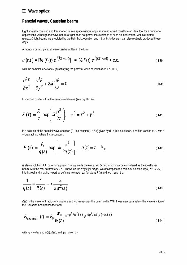
Confocal parameter, beam divergence The rate of increase is relatively small for IzI ≤ zR with w(zR) = 2 w0. If a Gaussian beam is focused down to a waist and than expands again (Fig. III-22), the full distance between the 2 w0 beam radii, within which the beam can be considered as nearly collimated, the depth of focus, is known as the confocal parameter of the Gaussian beam and given by

2022 R

wb z π= =

λ (III-50)

For IzI >> zR (often referred to as the far field of the beam), the beam radius increases at a nearly constant rate with distance from the waist, defining a cone with a half-angle, which – by using (III-45) and (III-48) – can be written as

0wλ

θ =π

(III-51)

and is called the divergence of the Gaussian beam.

Fig. III-22 Phase, Gouy-effect, wavefront The phase of the Gaussian beam

( )2

( , ) ( )2

kz kz zR zρ

φ ρ = −ϕ + (III-52)

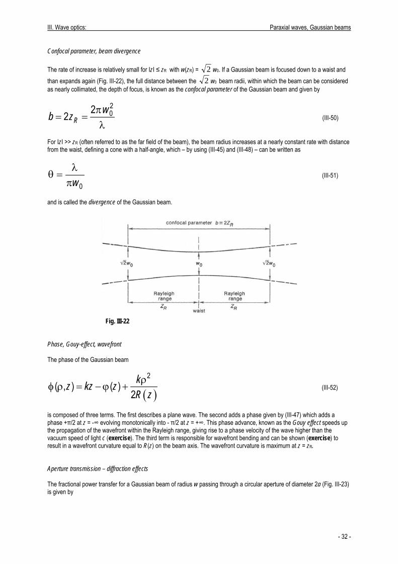
is composed of three terms. The first describes a plane wave. The second adds a phase given by (III-47) which adds a phase +π/2 at z = -∞ evolving monotonically into - π/2 at z = +∞. This phase advance, known as the Gouy effect speeds up the propagation of the wavefront within the Rayleigh range, giving rise to a phase velocity of the wave higher than the vacuum speed of light c (exercise). The third term is responsible for wavefront bending and can be shown (exercise) to result in a wavefront curvature equal to R(z) on the beam axis. The wavefront curvature is maximum at z = zR. Aperture transmission – diffraction effects The fractional power transfer for a Gaussian beam of radius w passing through a circular aperture of diameter 2a (Fig. III-23) is given by

- 32 -

III. Wave optics: Paraxial waves, Gaussian beams

2 2 2 22 / 2 /transmitted

20 0

2 2 1a

wP e d eP w

− ρ −= πρ ρ = −π ∫ a w

(III-53)

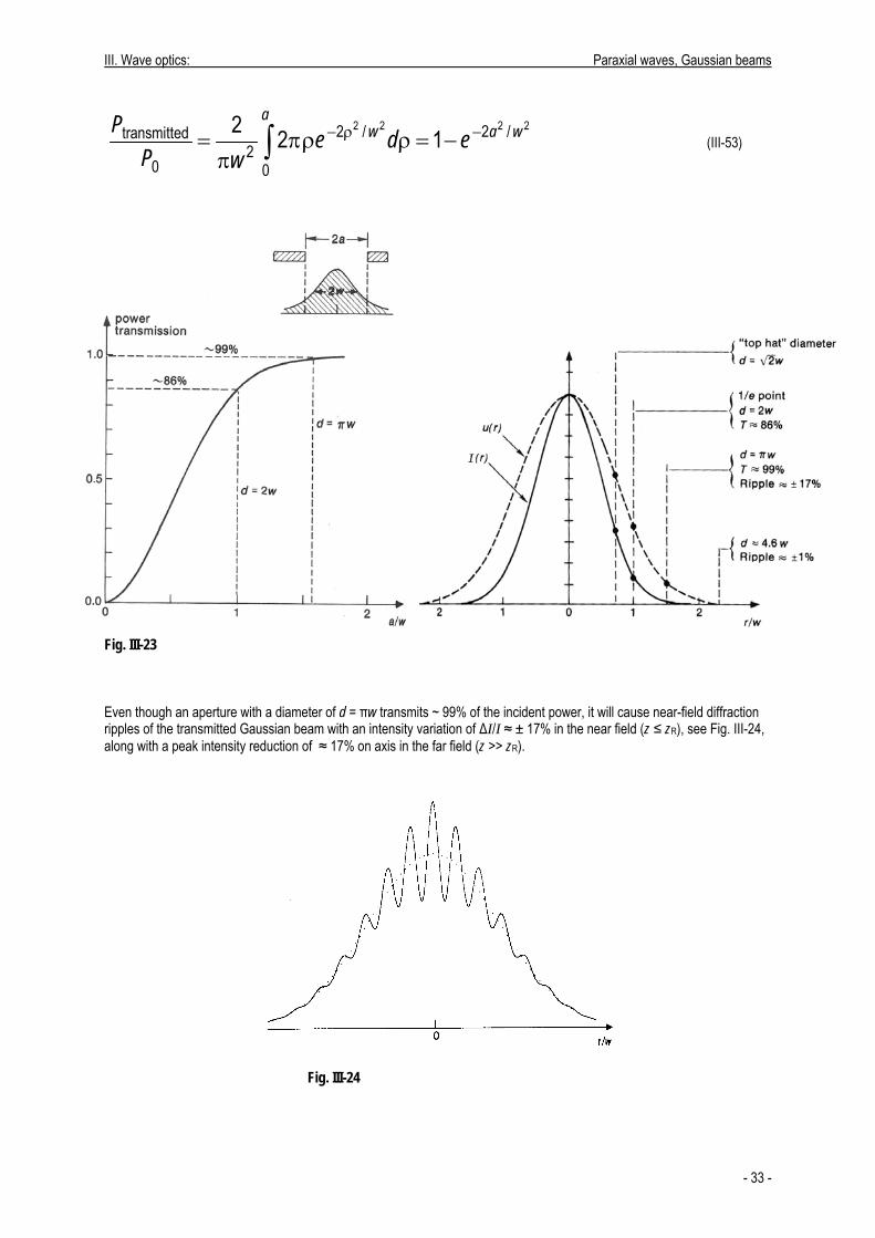
Fig. III-23 Even though an aperture with a diameter of d = πw transmits ~ 99% of the incident power, it will cause near-field diffraction ripples of the transmitted Gaussian beam with an intensity variation of ΔI/I ≈ ± 17% in the near field (z ≤ zR), see Fig. III-24, along with a peak intensity reduction of ≈ 17% on axis in the far field (z >> zR).

Fig. III-24

- 33 -

III. Wave optics: Paraxial waves, Gaussian beams

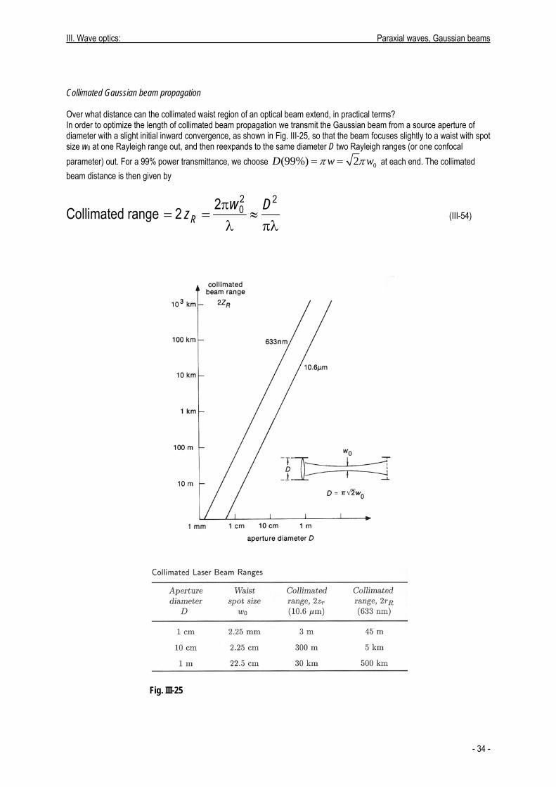
Collimated Gaussian beam propagation Over what distance can the collimated waist region of an optical beam extend, in practical terms? In order to optimize the length of collimated beam propagation we transmit the Gaussian beam from a source aperture of diameter with a slight initial inward convergence, as shown in Fig. III-25, so that the beam focuses slightly to a waist with spot size w0 at one Rayleigh range out, and then reexpands to the same diameter D two Rayleigh ranges (or one confocal parameter) out. For a 99% power transmittance, we choose 0(99%) 2D w wπ π= = at each end. The collimated beam distance is then given by

Collimated range 2 2022 R

w Dz π= = ≈

λ πλ (III-54)

Fig. III-25

- 34 -

III. Wave optics: Paraxial waves, Gaussian beams

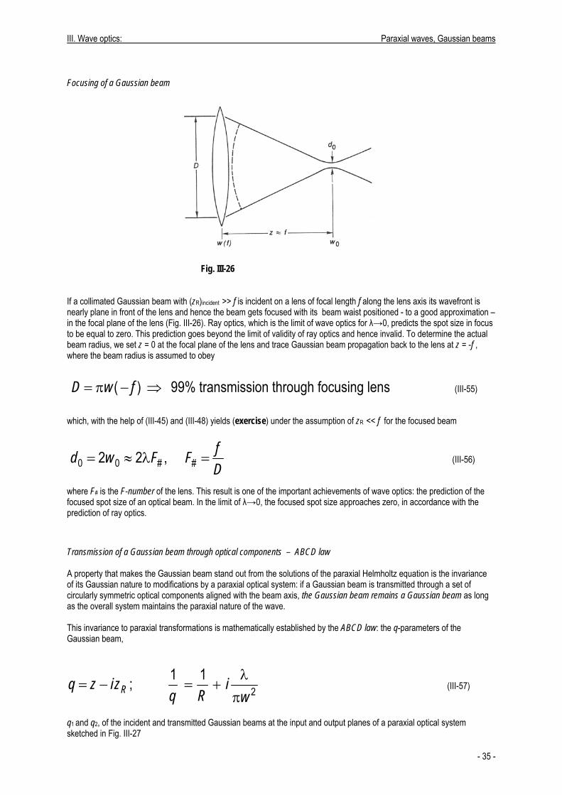
Focusing of a Gaussian beam

Fig. III-26 If a collimated Gaussian beam with (zR)incident >> f is incident on a lens of focal length f along the lens axis its wavefront is nearly plane in front of the lens and hence the beam gets focused with its beam waist positioned - to a good approximation – in the focal plane of the lens (Fig. III-26). Ray optics, which is the limit of wave optics for λ→0, predicts the spot size in focus to be equal to zero. This prediction goes beyond the limit of validity of ray optics and hence invalid. To determine the actual beam radius, we set z = 0 at the focal plane of the lens and trace Gaussian beam propagation back to the lens at z = -f , where the beam radius is assumed to obey

99% transmission through focusing lens (III-55) ( )D w f= π − ⇒

which, with the help of (III-45) and (III-48) yields (exercise) under the assumption of zR << f for the focused beam

0 0 # #2 2 , fd w F FD

= ≈ λ = (III-56)

where F# is the F-number of the lens. This result is one of the important achievements of wave optics: the prediction of the focused spot size of an optical beam. In the limit of λ→0, the focused spot size approaches zero, in accordance with the prediction of ray optics.

Transmission of a Gaussian beam through optical components – ABCD law A property that makes the Gaussian beam stand out from the solutions of the paraxial Helmholtz equation is the invariance of its Gaussian nature to modifications by a paraxial optical system: if a Gaussian beam is transmitted through a set of circularly symmetric optical components aligned with the beam axis, the Gaussian beam remains a Gaussian beam as long as the overall system maintains the paraxial nature of the wave. This invariance to paraxial transformations is mathematically established by the ABCD law: the q-parameters of the Gaussian beam,

21 1;Rq z iz iq R w

λ= − = +

π (III-57)

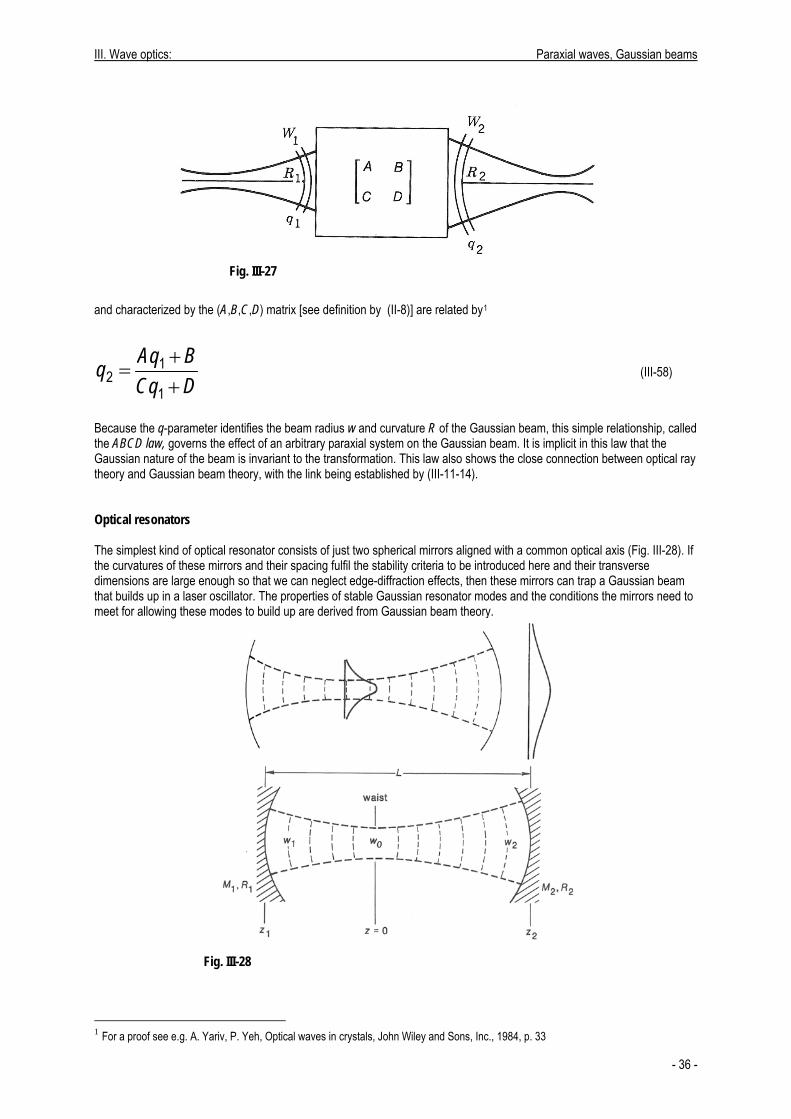
q1 and q2, of the incident and transmitted Gaussian beams at the input and output planes of a paraxial optical system sketched in Fig. III-27

- 35 -

III. Wave optics: Paraxial waves, Gaussian beams

Fig. III-27

and characterized by the (A,B,C,D) matrix [see definition by (II-8)] are related by1

12

1

Aq BqCq D

+=

+ (III-58)

Because the q-parameter identifies the beam radius w and curvature R of the Gaussian beam, this simple relationship, called the ABCD law, governs the effect of an arbitrary paraxial system on the Gaussian beam. It is implicit in this law that the Gaussian nature of the beam is invariant to the transformation. This law also shows the close connection between optical ray theory and Gaussian beam theory, with the link being established by (III-11-14). Optical resonators The simplest kind of optical resonator consists of just two spherical mirrors aligned with a common optical axis (Fig. III-28). If the curvatures of these mirrors and their spacing fulfil the stability criteria to be introduced here and their transverse dimensions are large enough so that we can neglect edge-diffraction effects, then these mirrors can trap a Gaussian beam that builds up in a laser oscillator. The properties of stable Gaussian resonator modes and the conditions the mirrors need to meet for allowing these modes to build up are derived from Gaussian beam theory.

Fig. III-28

1 For a proof see e.g. A. Yariv, P. Yeh, Optical waves in crystals, John Wiley and Sons, Inc., 1984, p. 33

- 36 -

III. Wave optics: Paraxial waves, Gaussian beams

If the radii of curvature of the mirrors in Fig. III-28 are exactly matched to the wavefront radii of the Gaussian beam at those points and if the transverse size of the mirrors is substantially larger than the spot size of the beam at the mirrors, each of these mirrors will reflect the beam exactly back on itself, with exactly reversed wavefront and direction, trapping thereby the beam as a standing wave between the mirrors. The two mirrors thus form an optical resonator for Gaussian modes of selected frequency (the eigenfrequencies of the resonator). In practice, the question is often asked the other way round: given the two-mirror resonator with parameters revealed in Fig. III-28 determine the Gaussian beam that will just properly fit between these two mirrors. The equations from which the position of the waist and the Rayleigh range of the Gaussian beam can be determined are as follows:

2

1 11

( ) RzR z z Rz

= + = − 1 R1, R2 > 0 (III-59a) for mirrors concave inward

2

2 22

( ) RzR z z Rz

= + = + 2

1

(III-59b)

2L z z= − (III-59c) Before solving the above set of simple algebraic equations, it is customary to define a pair of “resonator g parameters,” g1 and g2, which have become standard in the theory of laser resonators since the early years of lasers:

1 21 2

and1 L Lg gR R

≡ − ≡ −1 (III-60)

We can then find the trapped Gaussian beam from Eqs. (III-59a,b,c) and express the unique solution of these equations in terms of the g parameters: the Rayleigh length zR, which determines the waist radius w0

− λ= =

π+ −2 21 2 1 2

021 2 1 2

(1 ) ,( 2 )

RR

g g g g zz Lg g g g

2w (III-61)

and the position of the beam waist

2 11

1 2 1 2

(1 )2

g gz Lg g g g

−=

+ −and 1 2

21 2 1 2

(1 )2

g gzg g g g

L−=

+ − (III-62)

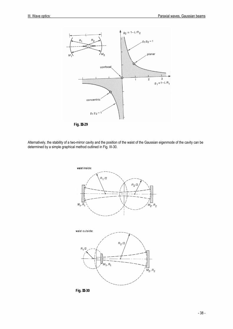
From these expression it is obvious that real and finite solutions for the Gaussian beam parameters exist only if the g1, g2 parameters are confined to a stability range defined by

1 20 g g≤ 1≤ (III-63) And depicted by the stability diagram in Fig. III-29.

- 37 -

III. Wave optics: Paraxial waves, Gaussian beams

Fig. III-29 Alternatively, the stability of a two-mirror cavity and the position of the waist of the Gaussian eigenmode of the cavity can be determined by a simple graphical method outlined in Fig. III-30.

Fig. III-30

- 38 -

III. Wave optics: Paraxial waves, Gaussian beams

Resonance frequencies The phase of a Gaussian beam (see III-52) at the resonator mirrors at points on the optical axis (ρ = 0)

1 1 1 2 2 2(0,z ) ( ), (0, ) ( )k z z z k z zφ = −ϕ φ = −ϕ (III-64) As the mirror surface coincides with the wavefronts, all points on each mirror share the same phase. Upon a complete round trip in the resonator, the Gaussian beam suffers a phase change of

[ ]round trip 2 1 2 1 2 12 ( ) 2 ( ) ( ) 2 2 , ( ) ( )k z z z z kL z z−Δφ = − − ϕ −ϕ = − Δϕ Δϕ = ϕ −ϕ

(III-65)

In order that the beam truly retraces itself, leading to a standing wave with a stationary amplitude distribution in the resonator (i.e. form a mode of the resonator), the round-trip phase change must be a multiple of 2π: ΔΦround-trip = 2πq, q = 0, ±1, ±2,….Substituting k = 2πνn/c and Δνax = c/2Ln, the frequencies that satisfy this condition are

q axq Δϕν = Δν + Δν

π ax (III-66)

and called the Gaussian-mode eigenfrequencies of the resonator. The frequency spacing of adjacent (axial) modes is equal to the inverse round-trip time of the resonator. Hermite-Gaussian beams It can be shown that

,mUl (r)2 / 2 (z) ( 1) ( )0

,22

(z) (z) (z)ikz ik R i m z

m myw xF G G x e

w w w+ ρ − + + ϕ⎡ ⎤⎡ ⎤

= ⎢ ⎥⎢ ⎥⎢ ⎥⎣ ⎦ ⎣ ⎦

ll l (III-67)

is also solution of the paraxial Helmholtz equation, where

2 / 2( ) ( ) , 0,1,2uG u H u e−=l l l ...=

1

(III-68) is known as the Hermite-Gaussian function of order Here stands for a Hermite polynomial defined by the recurrence relation

.l lH

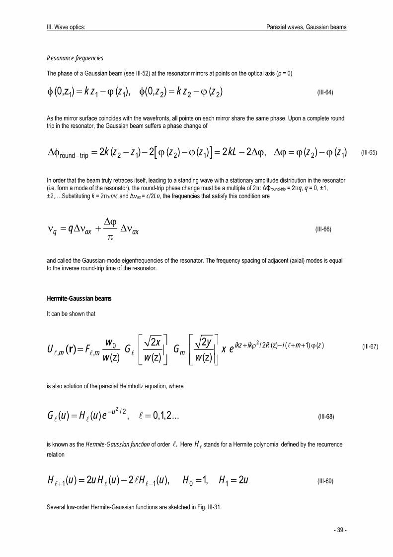
1 1 0( ) 2 ( ) 2 ( ), 1,H u u H u H u H H+ −= − =l l ll 2u= (III-69) Several low-order Hermite-Gaussian functions are sketched in Fig. III-31.

- 39 -

III. Wave optics: Paraxial waves, Gaussian beams

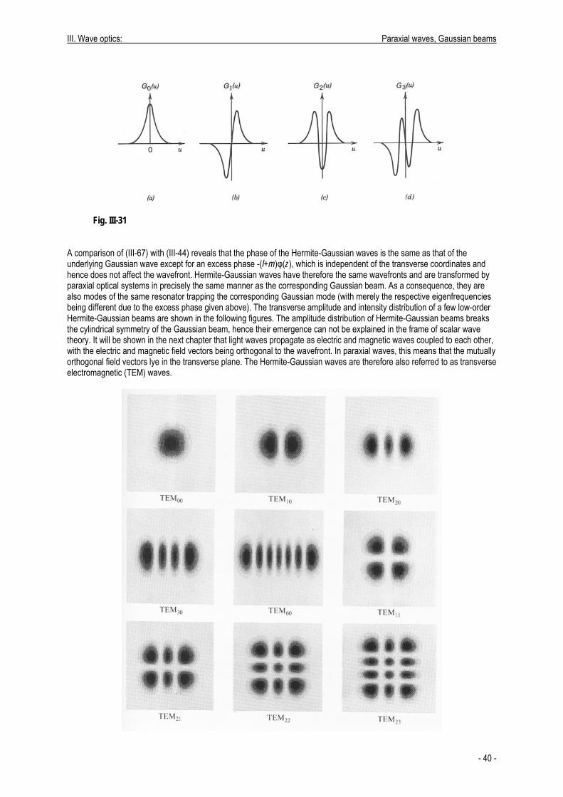
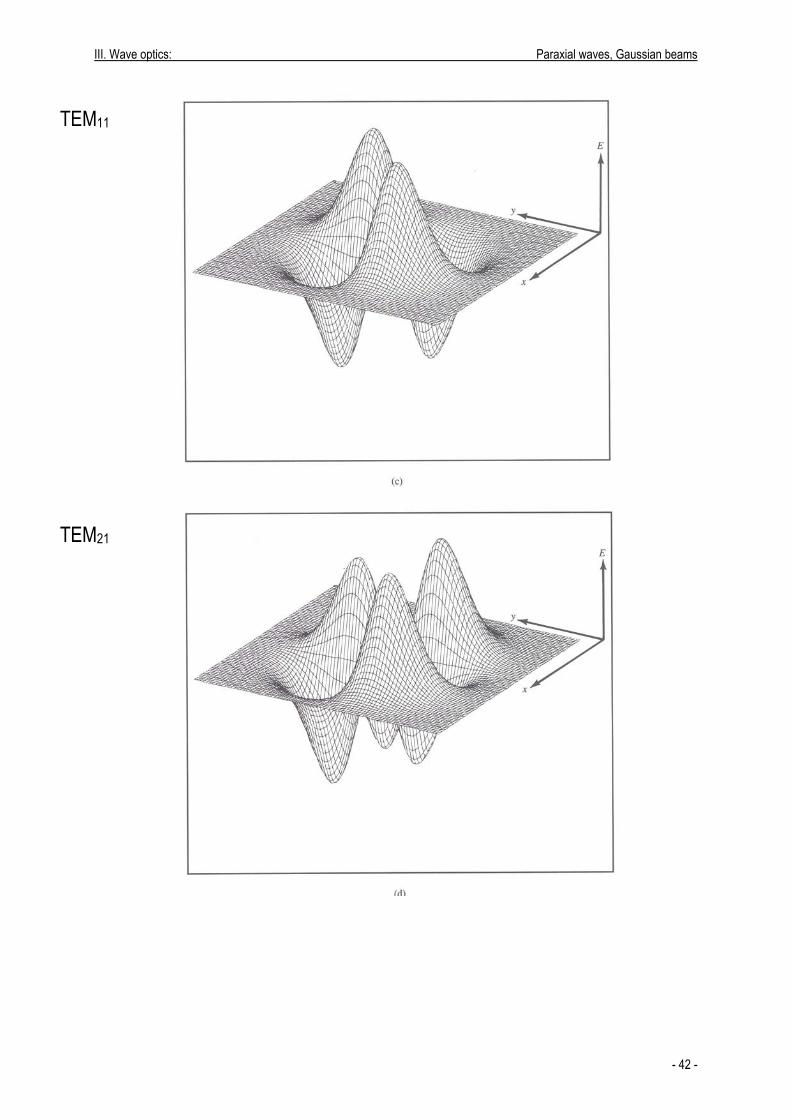
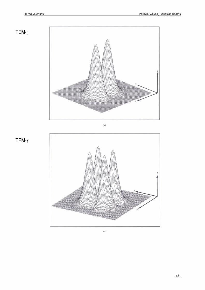
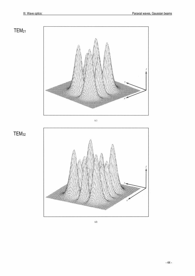
Fig. III-31 A comparison of (III-67) with (III-44) reveals that the phase of the Hermite-Gaussian waves is the same as that of the underlying Gaussian wave except for an excess phase -(l+m)φ(z), which is independent of the transverse coordinates and hence does not affect the wavefront. Hermite-Gaussian waves have therefore the same wavefronts and are transformed by paraxial optical systems in precisely the same manner as the corresponding Gaussian beam. As a consequence, they are also modes of the same resonator trapping the corresponding Gaussian mode (with merely the respective eigenfrequencies being different due to the excess phase given above). The transverse amplitude and intensity distribution of a few low-order Hermite-Gaussian beams are shown in the following figures. The amplitude distribution of Hermite-Gaussian beams breaks the cylindrical symmetry of the Gaussian beam, hence their emergence can not be explained in the frame of scalar wave theory. It will be shown in the next chapter that light waves propagate as electric and magnetic waves coupled to each other, with the electric and magnetic field vectors being orthogonal to the wavefront. In paraxial waves, this means that the mutually orthogonal field vectors lye in the transverse plane. The Hermite-Gaussian waves are therefore also referred to as transverse electromagnetic (TEM) waves.

- 40 -

III. Wave optics: Paraxial waves, Gaussian beams

TEM00

TEM10

- 41 -

III. Wave optics: Paraxial waves, Gaussian beams

TEM11

TEM21

- 42 -

III. Wave optics: Paraxial waves, Gaussian beams

TEM10

TEM11

- 43 -

III. Wave optics: Paraxial waves, Gaussian beams

- 44 -

TEM21

TEM32