CHARACTERIZATION OF SHAPE MEMORY POLYMERS FOR USE AS A MORPHING AIRCRAFT SKIN MATERIAL Thesis Submitted to The School of Engineering UNIVERSITY OF DAYTON in Partial Fulfillment of the Requirements for The Degree Master of Science in Aerospace Engineering by Robert Sebastian Bortolin UNIVERSITY OF DAYTON Dayton, OH August 2005
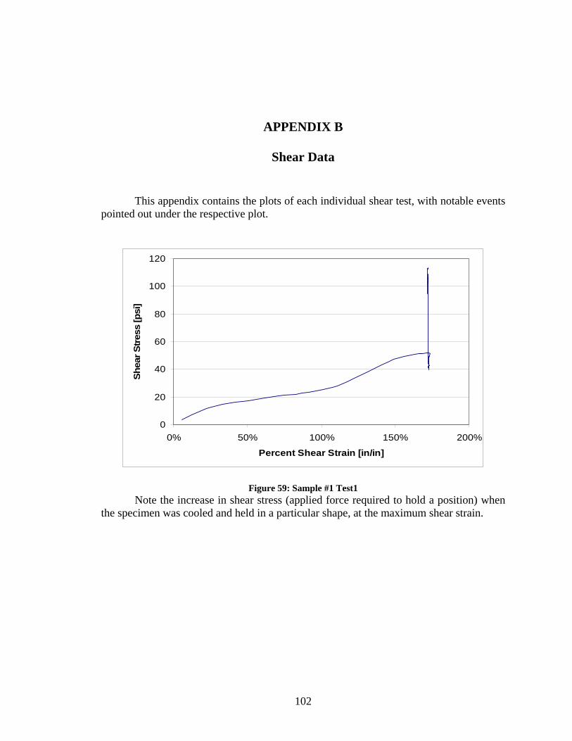
Transcript
CHARACTERIZATION OF SHAPE MEMORY POLYMERS FOR USE AS A MORPHING AIRCRAFT SKIN MATERIAL
Thesis
Submitted to
The School of Engineering
UNIVERSITY OF DAYTON
in Partial Fulfillment of the Requirements for
The Degree
Master of Science in Aerospace Engineering
by
Robert Sebastian Bortolin
UNIVERSITY OF DAYTON
Dayton, OH
August 2005
ii
CHARACTERIZATION OF SHAPE MEMORY POLYMERS FOR USE AS A MORPHING AIRCRAFT SKIN MATERIAL
APPROVED BY:
_______________________________ _________________________________ Brian Sanders, Ph.D. Geoffrey J. Frank, Ph.D. Advisory Committee Chairman Committee member Adjunct Professor, Mechanical and University of Dayton Research Institute Aerospace Engineering Department
_________________________________ _________________________________ Margaret Pinnell, Ph.D. Kevin Hallinan, Ph.D. Committee member Chair, Department of Mechanical and Assistant Professor, Mechanical and Aerospace Engineering Department Aerospace Engineering Department
_________________________________ _________________________________ Donald L. Moon, Ph.D. Joseph E. Saliba, Ph.D., P.E. Associate Dean Dean, School of Engineering Graduate Engineering Programs & Research School of Engineering
iii
ABSTRACT
CHARACTERIZATION OF SHAPE MEMORY POLYMERS FOR USE AS A MORPHING AIRCRAFT SKIN MATERIAL Bortolin, Robert S. University of Dayton Advisor: Dr. Brian Sanders
The research presented in this thesis investigated the characteristics of Shape
Memory Polymers (SMPs) for potential use as a skin material on morphing aircraft. Out
of the many possible morphing techniques to investigate, this research centered on in-
plane morphing, which provides the skin with a varying geometry while it must resist the
aerodynamic and structural loads presented to it. For this geometry change, it is necessary
to understand the behavior of the material in shear, as that is how the material will be
deformed. The shear properties were obtained by designing a unique test fixture to induce
pure shear in the SMP. With this fixture, the rate dependence of the material, the amount
of prestrain in the material and varying specimen geometry were tested in order to assist
in the understanding of the behavior of the SMP in shear. Additionally, a Finite Element
(FE) analysis was conducted to better comprehend the observed experimental results. The
tests showed that the behavior of the SMP was that of a nonlinear viscoelastic material,
indicating a high strain rate dependence of the material properties. There was a large out-
of-plane deformation noticed during the testing, and with the use of the FE model it was
iv
possible to identify this as buckling of the material. The results indicated that shape
memory polymers are a young technology in need of more research if they are to be used
for morphing aircraft skins. The end result is that SMPs are still a strong candidate
material for long term goals, but not enough is known about them for their use in the near
future as a deformable skin.
v
ACKNOWLEDGEMENTS
Special Thanks to Dr. Brian Sanders, my advisor, for directing my efforts over the
past year on something of such interest to me, and keeping me on track through the
months.
I would also like to thank the other committee members, Geoff Frank and Margaret
Pinnell, for their efforts in assisting me along the way.
Additionally, I want to thank Geoff for his wisdom and guidance throughout the
modeling process; Mrs. Michelle Keihl, for her early work with me and helping with the
organization of the testing; Brian Smyers for use of his lab, and taking the time to
introduce me to their control programs; Richard Wiggins for help with constructing the
environmental chamber and specimen preparation; Ernie Havens and Chris Hemmelgarn
at Cornerstone Research Group for providing the materials; and Dr. Shiv Joshi for
supplying a practical geometry over which to test the SMP
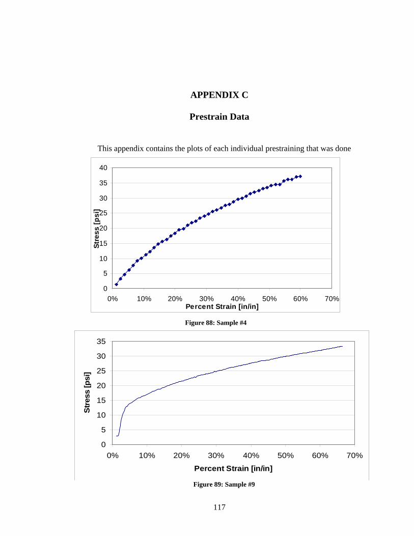
APPENDIX A: Geometric Relations Used to Calculate Shear Stress ....................... 99 APPENDIX B: Shear Data........................................................................................... 102 APPENDIX C: Prestrain Data .................................................................................... 117 APPENDIX D: Tensile Data ........................................................................................ 120 VITA............................................................................................................................... 128
vii
LIST OF FIGURES Figure 1: Aircraft with Variable Sweep Wings. Left to Right: F-111, B-1, F-14 ............. 1 Figure 2: Effect of Sweep on Drag vs. Mach Number ...................................................... 2 Figure 3: Spider Plot .......................................................................................................... 3 Figure 4: Out-of-Plane and In-Plane Morphing Aircraft Concepts ................................... 5 Figure 5: SAMPSON Lip / Flexskin / Cowl Geometry................................................... 13 Figure 6: Smart Wing Phase II Wind Tunnel Model....................................................... 15 Figure 7: Two Different Configurations of the Smart Wing Control Surface................. 16 Figure 8: Mechanical Response Curves of Various Materials to an Imposed Constant Force .......................................................................................................................... 22 Figure 9: Typical Modulus vs. Temperature Plot for an SMP......................................... 24 Figure 10: MTS 858 Table Top Load Frame................................................................... 28 Figure 11: Front and Back View of Experimental Set-up ............................................... 31 Figure 12: Prestraining Fixtures....................................................................................... 31 Figure 13: Shear Test Fixture .......................................................................................... 32 Figure 14: Geometry Changes and Associated Area Changes ........................................ 33 Figure 15: SMP in Shear Fixture; Not Clamped.............................................................. 33 Figure 16: SMP Bulk Sheet ............................................................................................. 34 Figure 17: ASTM D-638 Type I Specimen Geometry .................................................... 35 Figure 18: Load Frame Setup for Tensile Testing ........................................................... 36 Figure 19: Resultants from a Unit Force.......................................................................... 38 Figure 20: Shear Force, in % of Applied Force ............................................................... 39 Figure 21: Extension from Load Frame Connecting the Fixture to the Load Cell .......... 39 Figure 22: Shear Fixture (Without Specimen), Setup to Run Diamond to Square Shear Test................................................................................................................... 40 Figure 23: Prestrained Specimen Showing Where Shear Specimens Are Cut ................ 41 Figure 24: Data from Monotonic Testing ....................................................................... 47 Figure 25: Final Shear Specimen Geometry.................................................................... 48 Figure 26: Stress-Strain Curve Showing Repeatability of Tests at 203°F....................... 49 Figure 27: Stress-Strain Curve at Each of Three Different Rates for Four Cycles Going From 90........................................................................................................... 51 Figure 28: Sample #2 after cycling.................................................................................. 52 Figure 29: Sample #4 Showing Relaxation at T>Tg, Before Deformation ..................... 52 Figure 30: Specimen #1, Strained then Cooled Under Displacement Control ................ 53 Figure 31: Samples #2 and #1 Showing Folding of SMP During Testing ...................... 55 Figure 32: Shear Stress vs. Strain for samples in shear with different pre-strain............ 56 Figure 33: Illustration of Test Fixture Changes Which Induce Strain in the Sample...... 57 Figure 34: Samples with Increasing Prestrain, From Left to Right (0%, 28%, 60%) Recovered to Their Original Shape after Testing ..................................................... 58
viii
Figure 35: Specimen 12 after Tearing During Heating ................................................... 59 Figure 36: Requirements for Symmetric Bi-axial Prestrain ............................................ 59 Figure 37: Tensile Test After Specimen was Deformed and Cooled .............................. 61 Figure 38: Specimen 2 Fractured from Compression ...................................................... 61 Figure 39: Fracture Plot of Specimen 2 Cold .................................................................. 62 Figure 40: Shear Stress-Strain Curve for Sample 7, Cycled to 0.05” Displacement,
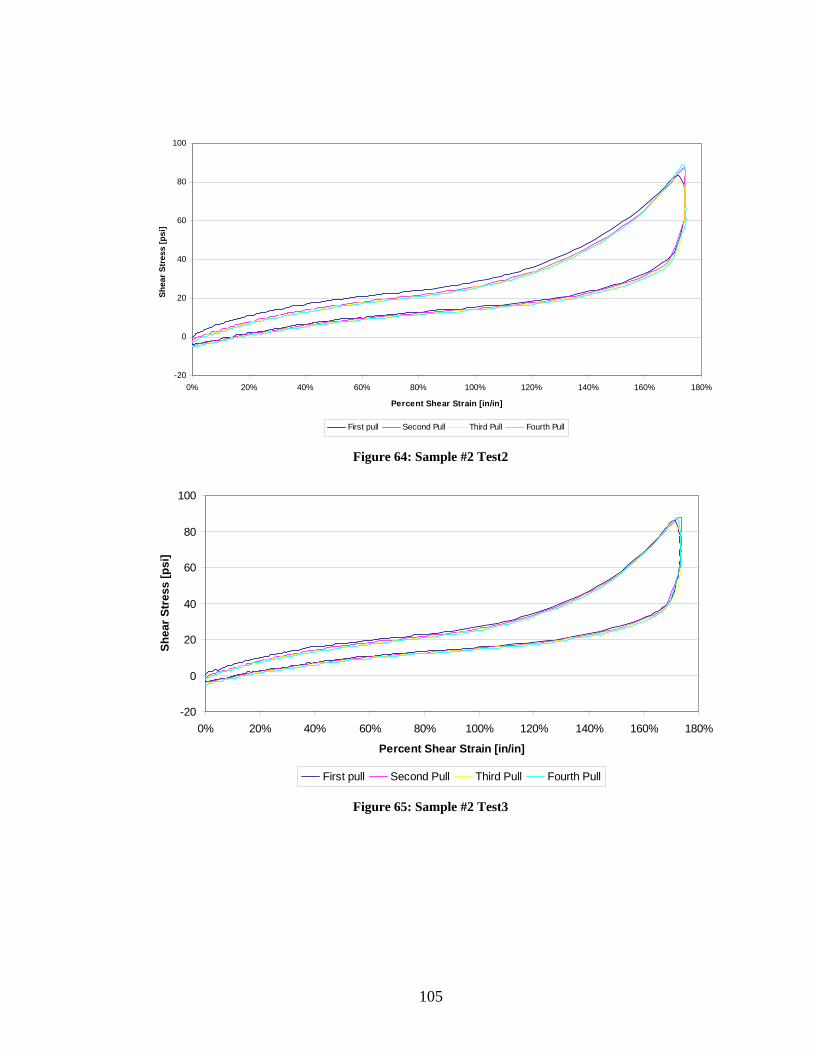
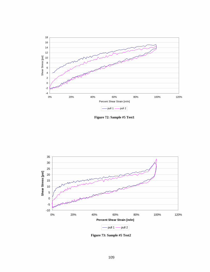
After Deformation and Cooling Below Tg ................................................................ 63 Figure 41: Shear Stress-Strain Curve for Sample 7 in Undeformed State, Cycled to 0.05” Displacement.................................................................................................... 64 Figure 42: Sample #5, Cold Cycled 25 Times................................................................. 65 Figure 43: Deformation Plots of Sample #7, Shown With Both Cycles from Sample #6 Test2......................................................................................................... 66 Figure 44: Tensile Data from 3 Tests at 2" /min Deformation Rate................................ 69 Figure 45: Tensile Results from Different Rates (Smoothed) ......................................... 70 Figure 46: Isochronous Stress-Strain Plots ...................................................................... 71 Figure 47: Drawing of the SMP / Fixture Used for Modeling & Early FEM Model .......................................................................................................................... 74 Figure 48: Stress-Strain Plot from Tensile Testing.......................................................... 75 Figure 49: Close-up of Element Failure........................................................................... 78 Figure 50: Modeling Stress-Strain Compared to Test Results......................................... 83 Figure 51: von Mises Stress Plot at a Displacement of 0.65 Inches ................................ 84 Figure 52: Two Views of First Eigenvector (Buckling Mode)........................................ 87 Figure 53: Force and Displacement Data from Model ................................................... 92 Figure 54: Folded Specimen ........................................................................................... 93 Figure 55: First (top) and Second (bottom) Mode Shapes Seen Together ...................... 93 Figure 56: Reaction Forces & Geometry ......................................................................... 99 Figure 57: Triangle Side and Angle Naming for Law of Sine's .................................... 100 Figure 58: Law of Sine's Definitions for Test Specimen............................................... 101 Figure 59: Sample #1 Test1 ........................................................................................... 102 Figure 60: Sample #1 Test2 ........................................................................................... 103 Figure 61: Sample #1 Test3 ........................................................................................... 103 Figure 62: Sample #1 Test4 ........................................................................................... 104 Figure 63: Sample #1 Cold Test .................................................................................... 104 Figure 64: Sample #2 Test2 ........................................................................................... 105 Figure 65: Sample #2 Test3 ........................................................................................... 105 Figure 66: Sample #2 Test4 ........................................................................................... 106 Figure 67: Sample #2 Test5 ........................................................................................... 106 Figure 68: Sample #2 Cold Tension .............................................................................. 107 Figure 69: Sample #2 Cold Compression ...................................................................... 107 Figure 70: Sample #3 Test1 ........................................................................................... 108 Figure 71: Sample #4 Test1 ........................................................................................... 108 Figure 72: Sample #5 Test1 ........................................................................................... 109 Figure 73: Sample #5 Test2 ........................................................................................... 109 Figure 74: Sample #5 Test3 ........................................................................................... 110 Figure 75: Sample #5 Test4 ........................................................................................... 110 Figure 76: Sample #5 Test5 ........................................................................................... 111
LIST OF TABLES Table 1: Tests and Test Variables, With Specimens Used…………………………………......40 Table 2: Summary of Comparison Test Results ............................................................... 43 Table 3: Basic Structural Material Properties of an SMP................................................. 68
1
CHAPTER I
INTRODUCTION
Starting with the first powered flight on 17 December 1903, humans have been
interested in changing the shape of aircraft for various reasons. Initially the Wright
brothers used wing warping for roll control, but as aircraft began moving faster structures
needed to become stiffer, making it harder for the wing to deform. Now aircraft are
controlled by distinct control surfaces using rigid body motion, such as flaps and ailerons
that change the lift characteristics of the wing, with minimal deformation of the structure.
More recently changes in wing shape have been used to improve the
aerodynamics of fighter aircraft. This can be observed in the variable sweep wings of the
F-14, B-1 and the F-111 in Figure 1. These wings allow the aircraft to have good
aerodynamics at multiple points in the flight envelope of the aircraft instead of optimal
performance at one point and poor to acceptable aerodynamics at other points. Most
noticeably swept wings reduces drag at higher Mach numbers, while long straight wings
Figure 1: Aircraft with Variable Sweep Wings. Left to Right: F-111, B-1, F-14
2
are better for performance at low speeds and generally increase the range and endurance
of an aircraft. Figure 2 illustrates how the coefficient of drag (CD) for a given wing
sweep angle increases with Mach number, but with an increase in wing sweep angle the
associated increase in the CD with Mach number is reduced. With variable sweep wings
an aircraft can combine the attributes of both straight and swept wings for increased
range over a swept wing aircraft and increased speed and maneuverability over a straight
winged aircraft.
The Air Force Research Laboratory defines morphing aircraft as aircraft that are
capable of large scale controlled deformation to allow for a change of state of the aircraft.
This change of state allows the aircraft to have improved aerodynamic performance
throughout its entire flight envelope, even when compared to multiple aircraft
simultaneously. This is because current aircraft are designed with a specific wing
geometry that provides optimal performance at one point in the flight envelope that is
Figure 2: Effect of Sweep on Drag vs. Mach Number Figure 2 used with Permission from www.aerodyn.org
3
considered the most critical point. Performance decreases drastically as the aircraft moves
away from that one point in the flight envelope.
Figure 3 shows what is called a spider plot. This plot compares how efficient
different configurations are for different phases of flight, though does not necessarily
show all possible flight regimes. The blue plot that almost fills the circle corresponds to
the morphing concept shown by the aircraft figures surrounding the circle. Each radial
line indicates a different phase of flight, such as take off, cruise, or maneuver, with more
efficient configurations filling more of the circle along that direction. As is easily seen
the blue plot is the most efficient of the three shown because it fills most of the circle.
The green plot bordered by the dashed line is the next smaller plot, representing a less
efficient aircraft design, possibly that of a variable sweep wing. The aircraft has good
efficiency at most points on the plot, but is not as good as the morphing concept. The
smallest plot, shown in red, is more representative of a typical aircraft design, with some
5 Cycled Shear Bulk 203 2.0 90 to 30 to 90 Repeatability 1 (X8), 2 (X16)
6 Cycled shear at varied rates
Bulk 203 0.2, 2.0, 20.0
90 to 45 to 90 Rate Dependency
5, 6
7 Extreme Reverse Shear
Bulk Room 0.05 90 to 87 Load Limit 1
8 Extreme Reverse Shear
New shape Room 3.0 45 to 27 Load Limit 2
9 Extreme Positive Shear
Bulk Room 0.05 90 to 68 Load Limit 5
10 Extreme Positive Shear
New shape Room 0.05 45 to 51 Load Limit 2
11 Low load, High cycle
Bulk Room 0.05 90 to 89 Repeatability, Shear Modulus
7 (X10) 5 (X25)
12 Low load, High cycle
New shape Room 0.05 45 to 43 Repeatability, Shear Modulus
7 (X10)
Figure 22: Shear Fixture (Without Specimen), Setup to Run Diamond to Square Shear Test
41
The initial tests were done monotonically, but could easily be reversed for cyclic
testing. For all of the shear tests, except those done on rate dependence, the specimen was
deformed at a rate of 2” per minute [Ram, 1997; Anon, 2005.]. As testing progressed it
was desired to run the test in the opposite direction as well, pulling the SMP from a
diamond to a square. Figure 22 shows how the same test fixture could easily be used, but
a new, taller, bottom grip was needed because the extension to the load frame was not
long enough to reach the specimens with the new geometry, and the bottom grip was
easier to fabricate.
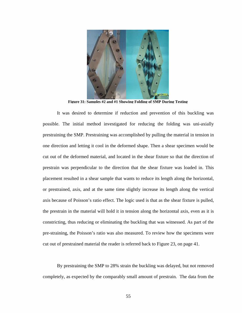
All the samples except sample #7 were allowed to recover to their original shape
between tests, either rapidly in a boiling water bath or slowly lying on the floor of the test
set-up environmental box during other testing at T>Tg. This was done so that each test
would begin with a flat specimen, even if it were not freshly cut from the bulk material.
Once the test process was validated by our initial tests it was expanded to include
some investigation of prestrain effects, cycling, and rate dependency of the SMP. Figure
23 shows prestrained material, with images of the shear test specimens drawn where they
Figure 23: Prestrained Specimen Showing Where Shear Specimens Are Cut
42
would be cut out. The arrows indicate the direction of the applied force during the shear
testing. The prestraining was accomplished with the tensile fixtures described above by
pulling a small sheet of the bulk material to a predetermined percent strain. The SMP was
then allowed to cool in this new shape, and the shear specimen was then cut out of the
material. The shear tests on these specimens were done so that the direction of prestrain
was perpendicular to the direction of tension for the shear tests. This was so that the
prestrain would be relaxed as the two sides of the shear fixture acted in compression on
the specimen.
The tensile specimens were cut from bulk material as received from Cornerstone
Research Group. All of the tests were performed on the same load frame as previously
described, with some preliminary comparison tests done elsewhere.
To perform the ASTM tensile testing, an accurate way to measure the strain was
needed in order to compute the modulus. Normally this is done with a laser extensometer
and reflective tape for polymers, but the cost of an extensometer prevented the purchase
of one for these experiments. A Tinius Olson load frame packaged with a laser
extensometer was available for some tests, but the laser would not be able to obtain data
when the specimen was in the oven attached to the load frame.
It was noted that Abrahamson, et al. [2002] had a similar problem with their work
on elastic memory composites. In their research, they showed that using the displacement
of the load frame crosshead to measure strain resulted in only a minor difference in the
43
strain, and that was only below approximately 3% strain. Above 3% strain data from a
video system and the crosshead were identical, and since they were concerned about data
at greater strains it was not crucial as to what measurement they used.
It was decided that, faced with a similar problem, a similar solution would be
sought. Having access to the Tinius Olson frame and laser extensometer combination
provided the means to run the tests. The software that came with the machine was not
able to read two displacement inputs, so multiple tests were run using each of the two
measurement devices. The results are tabulated below in Table 2, with the average and
standard deviation calculated as well. The “L” and “CH” columns indicate which method
was used to measure the displacement, Laser or CrossHead.
Table 2: Summary of Comparison Test Results
SMP E (psi) L CH 10 182139 x 11 204793 x 12 205000 x 13 180580 x 14 174890 x 15 202024 x 16 200338 x 17 176842 x 18 206279 x 20 217411 x 21 205663 x 22 205079 x 23 237000 x 24 202500 x
AVG modulus 200038.43 208456 193726
SD 16850 18456 13330
Based on these results, a correction factor for the specimen was calculated to be
1.076. As long as the tests use the same specimen geometry and distance between the
44
grips the correction factor holds true. This is more critical to these tests than the ones
mentioned above because these tests are concerned with the modulus as well as material
properties and reactions at other locations along the stress-strain curve.
To perform these tests, the cut specimens were clamped into the load frame with a
thermocouple taped to the specimen approximately one-third of the length from the
bottom. The output from this thermocouple was used to determine the temperature of the
specimen. There was a second thermocouple imbedded in the oven that was used to help
prevent overheating of the specimen from the oven becoming too hot. Once the straining
had begun, the thermocouple taped to the material came off, preventing the tape from
effecting the strength of the material.
The oven was closed around the specimen, with insulation added in the gap at the
side where the two halves of the oven locked together. The temperature was then set at
250° F for the thermocouple on the oven itself. When this value was obtained the set
point was increased to 265° F. Once the oven held stable at this temperature control was
switched to the thermocouple taped to the specimen, which at this point would be nearly
the desired 203° F.
This form of temperature control was used to prevent a large overshoot of the
desired temperature that was likely to occur because of the low conductivity of the
specimen and the rapid temperature change the occurred in the ovens heating elements. If
the thermocouple on the SMP were to be used alone the temperature within the oven
45
would be well over 300° F before the specimen was at temperature, and it would not cool
off quickly, and therefore continue to raise the temperature of the specimen well over the
desired test temperature, and possibly above the degradation temperature of the material.
Once the specimen was stable at the desired temperature the tensile test was
preformed, which involved the bottom of the specimen remaining fixed, while the top
was pulled out of the oven. While not desirable, this occurrence was inevitable because
the heating area of the oven was only four inches high. During testing at the slower rates
this could allow the material to cool enough to increase the stiffness slightly, which
would also drive up the calculated modulus at these rates as well. At higher rates the
material would not have enough time to cool off while the test was being conducted.
3.3 Chapter Summary
The above pages described the setup for the shear and tensile tests that were
performed, the items critical to the test in addition to the load frame, and the procedures
used during those tests. There were three fixtures designed to be used for the tests, two
for prestraining the material and one for the shear tests. In the end, to simplify data
acquisition, the same load frame was used for both kinds of testing, with the gripping
mechanism changed from pinning to hydraulic, and the heating device changed between
the environmental box and a small clamshell oven for the shear / prestrain tests and the
tensile tests, respectively.
46
CHAPTER IV
RESULTS
Chapter four discusses the experimental results of the individual
experiments that were conducted to obtain the shear properties of the material. These
properties are a function of the specimen geometry, the rate at which the specimen was
sheared, and how much the specimen was prestrained. This chapter will also show how
the desired properties were calculated from the experimental data.
4.1 Monotonic Shear Testing
In order to determine how well the test fixture worked the initial tests were
monotonic. By performing a simple test over the full range of shear strain, it was possible
to work out most of the problems that otherwise would have occurred during the more
important and complicated testing. This also allowed familiarization with the load frame
and the associated data acquisition and control software.
A small flaw in the specimen / fixture combination was noticed during the testing.
The specimen would begin folding almost as soon as the test began because the sides
were in compression. Beyond approximately 100% shear strain it was possible for the
folded specimen to become pinched in the fixture at one of the corners. This increased the
47
required force to continue to strain the specimen because in addition to straining the
specimen, the applied force also had to compress the folded specimen. This phenomenon
can be noted in Figure 24, “Specimen1_Test2” with a sharp increase in shear stress seen
starting at approximately 120% shear strain.
Moving past these learning experiences, data from the first specimen and third
specimen (after being prestrained 28%) was successfully obtained from the monotonic
testing. Figure 24 shows the data from these tests, with the specimen being pulled so that
the smaller interior angle was 30° at the end of the test, and the fixture was held briefly at
the resulting final strain. The first specimen tested shows a fairly smooth curve until it
begins to be pinched in the test fixture. The specimen that was prestrained has a plot that
can be divided up into three sections. The initial, linear, section, which lasts until 50%
shear strain; the second section is identified by the nearly constant stress until almost
100% shear strain; the last section is where the shear stress increases again, until
0
50
100
150
200
250
0% 20% 40% 60% 80% 100% 120% 140% 160% 180%
Percent Shear Strain [in/in]
She
ar S
tress
[psi
]
Sample3 - 28% Specimen1_Test2
Figure 24: Data from Monotonic Testing
48
maximum strain is obtained. This test will be discussed in more detail with other tests
done on prestrained specimens, in section 4.4.
To alleviate the pinching mentioned above it would be possible to run the tests to
only 100% shear strain (45° / 135° interior angles) but that would not cover the full range
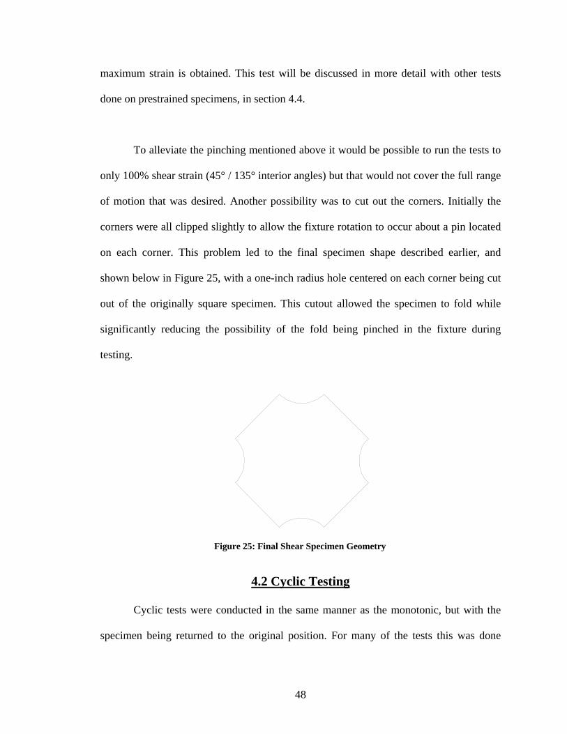
of motion that was desired. Another possibility was to cut out the corners. Initially the
corners were all clipped slightly to allow the fixture rotation to occur about a pin located
on each corner. This problem led to the final specimen shape described earlier, and
shown below in Figure 25, with a one-inch radius hole centered on each corner being cut
out of the originally square specimen. This cutout allowed the specimen to fold while
significantly reducing the possibility of the fold being pinched in the fixture during
testing.
4.2 Cyclic Testing
Cyclic tests were conducted in the same manner as the monotonic, but with the
specimen being returned to the original position. For many of the tests this was done
Figure 25: Final Shear Specimen Geometry
49
multiple times without cooling the specimen. The results from these tests indicated that
the test was highly repeatable.
Two different specimens went through a total of 24 cycles, with typical results
shown in Figure 26. To reduce clutter in the graph, stress-strain data for only two tests are
shown. The samples were cycled four times in the fixture without being cooled. All four
cycles of both specimens are essentially the same. The set of curves beginning near the
origin are from the loading portion of the test. Once the maximum strain was reached,
seen at the peak stress, the specimens were immediately returned to zero strain at the
same displacement rate. The curves for each test are continuous, dropping to negative
stress at low strains during the unloading portion of the test. The steep decline in shear
stress near the maximum strain shows that by simply removing some of the applied force
the material will reduce its strain. This plot indicates that not only is the test repeatable
between specimens, but also that the test does not change the properties of the SMP or
induce plastic strain, and that the specimens did not slip out of the fixture.
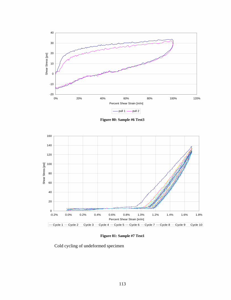
When undergoing the series of tests for the cold cycling, the SMP performed
similarly to other tests during the heated deformation process; but when it was heated to
be returned to its initial position, there was some discrepancy that can be seen in Figure
43. The start of the unloading curve, after sample #7 was cooled, cycled and reheated, is
much lower than the end of the loading curve. A potential source of error in this test was
the intermittent data acquisition; instead of gathering data constantly, it was collected
only during the actual testing. At least one hour is needed to both heat and cool the
specimen. Currently the temperature control is done by an external controller, not one
linked to the MTS machine. Had the data acquisition run the whole time, one would
notice an increase in force as the SMP cools as mentioned previously, and the force
would stabilize again once the SMP is well below its Tg, and no longer experiencing a
change in temperature. These force and temperature changes that were not recorded could
produce the difference in forces seen in the figure.
-10
-5
0
5
10
15
20
25
0% 20% 40% 60% 80% 100%
Percent Shear Strain [in/in]
She
ar S
tres
s [p
si]
Sample6_Test2_C1 Sample6_Test2_C2 Sample 7
Figure 43: Deformation Plots of Sample #7, Shown With Both Cycles from Sample #6 Test2
67
Since the natural aerodynamic loads deform a structure, the SMP will experience
load cycling similar to the low-load test. When this test is done on more samples, it can
be determined if the SMP will experience a permanent change or if it will recover
completely every time it is heated up. Should the SMP experience a permanent change,
over time it will be able to carry less of the shear loads. The implication for an aircraft
wing’s design is that it would require a stronger internal wing structure to prevent failure.
If the SMP recovers fully after heating, the structure can be designed to allow the SMP to
carry some of the shear loading, allowing the planform to change.
Each of the above described tests provided information on the properties of the
SMP. The averaged results for the basic material characteristics obtained from each test
are shown in Table 3. It is noted that prestraining the material appears to have an effect
on the shear modulus, though more tests are needed at each amount of prestrain to verify
the significance of prestrain on the modulus. Another important point is that if one were
to calculate the shear modulus from the tensile properties (E = 87 psi, ν = 0.28) it would
be slightly higher than the one listed in Table 3. The most likely cause of this is error in
the property measurements, especially in Poisson’s Ratio, as it was not measured in a
controlled experiment for tensile properties but rather was obtained during a prestraining
of the material, where the specific properties were not as important as the final shape
obtained.
68
Table 3: Basic Structural Material Properties of an SMP Shear Modulus, G, of bulk material at 203°F 25.8 +3.0 / - 3.5 psi
Shear Modulus, G, of pre-strained material – 28% pre-strain at 203°F
38.9 psi
Shear Modulus, G, of pre-strained material – 60% pre-strain at 203°F
28.8 psi
Shear Modulus, G, of bulk material at room temperature 17385 psi Poisson’s ratio from 60% pre-strain at 203°F 0.28 Extreme Positive Shear Load Limit to fracture with formed samples at room temperature
3855 psi
4.6 Tensile Test Results
Tensile tests were conducted to determine the modulus of the SMP over a range
of temperatures, determine the strain mechanism of the material. It was only possible to
conduct a few of the desired tensile tests, so the testing was limited to tests performed at
the same temperature at which the shear tests were performed. This would allow for an
improved value for the modulus at temperature to be determined, when compared to the
properties obtained from prestraining, but of primary interest was the ascertainment of
the materials reaction, be it linear or non-linear, and viscoplastic (VP) or viscoelastic
(VE.)
Of the five tensile tests that were run, three were done at a deformation rate of 2
inches per minute, which was the same rate used for the majority of the shear tests. The
stress-strain plots resulting from these tests are seen in Figure 44. After analyzing the
data it was found that the SMP provided for this research has a modulus of 87 psi when
heated to 203° F.
69
Generally, to determine the linearity of a materials strain behavior a specimen is
tested at multiple rates. The results are plotted on stress-time and strain-time graphs, and
at least one time of interest is used. The strain of the material from each rate, and the
corresponding stresses at this time are recorded, and plotted on what is called an
isochronous stress-strain plot. If the material is a linear viscoelastic the resulting stress-
strain plot will be linear, and pass through the origin. In order to determine linearity and
whether the material went through a VP or VE straining process two higher deformation
rates, each an order of magnitude faster than the last (2 inches per minute, 20 inches per
minute, 200 inches per minute,) were used (Figure 45.) The smoothed curves shown were
obtained by placing a curve fit over the data, then plotting the equation obtained from the
curve over the range of strain from the actual data.
-5
0
5
10
15
20
25
30
35
40
45
0% 10% 20% 30% 40% 50% 60% 70%Strain [in/in]
Stre
ss [p
si]
Test 2 Test 3 Test 4Figure 44: Tensile Data from 3 Tests at 2" /min Deformation Rate
70
The rates that these tests were performed at limited the times available at which
all three rates has useful data, as the first data point at the slowest rate corresponds to
nearly the last data point at the highest rate, preventing a large sampling range over which
the data could be used.
With the use of the curve fit equations used in Figure 45 stress-time and strain-
time plots were made, with the only overlapping physical data point being at a time of
0.0025 seconds. The resulting isochronous stress-strain plots are shown in Figure 46.
From Figure 46b one can see that the material is linear VE up to at least 5% strain. Figure
46a shows that somewhere between 5% and 50% strain the material goes nonlinear or
plastic. By testing other rates it would be possible to obtain data to fill in the spaces
between the data points on Figure 46 to confirm the linearity, and to determine where the
Figure 45: Tensile Results from Different Rates (Smoothed)
71
To determine if the SMP is VP or nonlinear VE is a simple matter of observing
what happens to the material when it is returned to zero strain. If, after a time, the
material returns to zero stress it would be considered a viscoelastic material. If it does not
return to zero stress, then there was some plastic deformation that occurred. The test can
also be conducted by returning the material to zero stress and waiting to see if it returns
to zero strain over time.
The shape memory effect of the SMP is such that, when above Tg and with no
applied load, the material will return to the initial shape that it was formed in, which was
a flat sheet for this research. Based on this knowledge, and observations made in
returning the material to its initial condition after tests, it would be safe to say that, at
temperature, SMPs are most likely a nonlinear viscoelastic material.
0
5
10
15
20
25
30
35
40
0% 15% 30% 45% 60% 75%
Strain [in/in]
Stre
ss [p
si]
0
0.5
1
1.5
2
2.5
3
3.5
4
4.5
5
0% 1% 2% 3% 4% 5% 6%
Strain [in/in]
Stre
ss [p
si]
0
5
10
15
20
25
30
35
40
0% 15% 30% 45% 60% 75%
Strain [in/in]
Stre
ss [p
si]
0
0.5
1
1.5
2
2.5
3
3.5
4
4.5
5
0% 1% 2% 3% 4% 5% 6%
Strain [in/in]
Stre
ss [p
si]
a) All Data Points b) First Two Data Points Figure 46: Isochronous Stress-Strain Plots
72
4.7 Chapter Summary
This chapter broke down the results of the various experiments performed,
describing the behavior of SMPs. Some observations were made during the testing that
were not expected, so the tests were expanded to help understand these phenomena. At
the end of the chapter there is a table summarizing the results from the shear testing,
which indicate the SMPs ability to function structurally. The final section, on the tensile
tests, provides a more accurate value of the modulus of the SMP at temperature, and
evidence for SMPs to be a nonlinear viscoelastic material, when heated above their Tg.
73
CHAPTER V
MODELING
A Finite Element (FE) analysis was conducted to aid in the understanding of the
experimental analysis. PATRAN was used as the visual interface, and ABAQUS used to
do the nonlinear material analysis. Even though the model was symmetric, due to the
translational complexity of the problem, and it’s comparably small size, a full model was
used. The model build up, various constants, elements used and the process in going from
the initial elastic model to a more accurate elastic-plastic model are explained.
Additionally, a buckling analysis was done to determine at what force and displacement
buckling would occur in the model, if at all.
5.1 Basic Geometry and Model Development
Figure 47 shows the FE model, and an example mesh. The outer square in the
figure represents the fixture, while the other areas represent the material. In the cutout at
each corner there is no material, as is noticed by the lack of mesh for those regions on the
right side of the figure.
74
The model was initially meshed with the automatic edge length calculation
feature in PATRAN recommending an edge length for the elements. This was done for
all of the surfaces and all of the curves that were meshed. The surfaces were all meshed
with two dimensional shell elements. The edge surfaces, where the SMP was held into
the fixture, had a thickness of 0.5 inches and a modulus of 29,000,000 psi, which is the
modulus of steel. This was done to represent the fact that the SMP was being held rigidly
between two pieces of steel. The rest of the SMP was modeled with a thickness of 0.154
inches, which is equivalent to 4 mm. As the model progressed data from prestraining the
SMP 60% was used to obtain a value of 115 psi for the modulus of the SMP. This value
was used on all models until the tensile testing was completed, which provided a slightly
lower modulus of 87 psi (Figure 48).
Figure 47: Drawing of the SMP / Fixture Used for Modeling & Early FEM Model
75
The fixture was modeled with the B31 element in ABAQUS, which is a one-
dimensional beam element. These elements were given a cross-sectional area of 0.45 in2
and a moment of inertia of 0.0152 in4.
The model is made of multiple areas, and each area must be meshed separately,
creating extra nodes where the surfaces met, or where surfaces and curves, which
represent the fixture, overlapped. Once the model was meshed all nodes that were
meshed twice had to have the second mesh removed. Removing these duplicate nodes
essentially glues the different areas, or areas and curves, together, creating a solid model.
In order to allow the fixture to move realistically, rotating around the corners, each corner
needed to have two nodes to represent the two different sides of the fixture. If a corner
had only one node it would be equivalent to making that corner rigid instead of making it
0
5
10
15
20
25
30
0% 10% 20% 30% 40% 50%
Percent Strain [in/in]
Stre
ss [p
si]
Figure 48: Stress-Strain Plot from Tensile Testing
76
out of two bars pinned together. This resulted in all of the duplicate nodes, except those at
the four corners, being removed.
Since the four sides of the fixture were now modeled as four separate entities they
had to be pinned at their corners. This was done with the use of Multi-Point Constraints
(MPCs.) An MPC requires that motion of a set of independent nodes be exactly copied by
the set of dependant nodes. Four MPCs were used, one for both the ‘x’ and ‘y’ directions
at each of the two side corners.
To prevent the model from pure translation the two bottom nodes were
constrained from all motion except rotation about the ‘z’, or out-of-plane axis. The
corners on the two sides were constrained from out-of-plane translational motion, while
allowing a rotation about the ‘z’ axis only. The top corner of the model was only allowed
to move vertically, or in the ‘y’ direction, while the only allowable rotation was once
again about the ‘z’ axis. These boundary conditions ensured that the model would rotate
about pinned corners, with motion of the fixture in the x-y plane only. Finally, a
displacement was prescribed at the top corner. This displacement was originally only one
inch to validate the model, but as the model progressed the displacement was increased to
2.07 inches, which was the final displacement in the shear tests, and resulted in an
interior angle of 30o at the top and bottom corners.
Many model iterations were required to advance the fidelity of the FE model due
to the complexity of the test being modeled and in properly quantifying the actual
77
properties of the material for the analysis. The FE analysis was first done on a purely
elastic material, with the thought that as the model was refined the material would
progress to an elastic-plastic model, and finally some form of a viscoelastic-viscoplastic
model, based on the properties obtained from the testing that was conducted in parallel
with the modeling.
The first models used S4R5 elements for the shells. This indicates that the shells
had four nodes, used reduced integration, and were allowed five degrees of freedom.
Reduced integration means that the element stiffness matrix was calculated with a lower
order integration, which greatly reduces running time for large analyses. Generally
speaking, instead of using four points within the element for integration, only one is used.
This method also often provides more accurate results when the elements are not
distorted [ABAQUS, 1995].
Initially the models had a singularity at the boundary between the two material
models of the SMP. There was an increase of modulus of multiple Orders Of Magnitude
(OOM’s) at the intersection, as well as a thickness change, because the edge of the SMP
was modeled as being the steel fixture since it was held rigidly. This singularity caused
the softer elements on the boundary to deform greatly and eventually enough that the
element could not be integrated across and the analysis had to be stopped.
The modeling progressed with a few small changes at each iteration to improve
the fidelity of the model and ensure the proper inputs to ABAQUS. The next model had
78
the mesh refined to approximately one third the size suggested by the automatic edge
length calculation feature. The initial displacement was set to 0.05 inches to ensure that
the model would run. Once the model ran smoothly the next model was made with no
changes, other than increasing the desired displacement to the full 2.07 inches. Failure
occurred at approximately 0.5 inches of displacement, with the softer elements at the
singularity deforming beyond use. This is the failure mechanism for the analysis at every
iteration unless otherwise noted.
Figure 49 shows part of the model and a close-up of a corner where the elements
failed. All of the blue lines on the left picture indicate different elements. In the close-up
one can see the individual element shapes. All of the elements were initially square like
the elements at the top or bottom of the figure. At the material discontinuity it is easy to
see that the soft elements deformed significantly to various forms of trapezoids and
triangles. When the elements degrade to triangles and beyond (arrowhead shapes),
usually from the straining of the material, the stress and strain equations that are solved
for the element can no longer be solved, preventing the analysis from continuing.
Figure 49: Close-up of Element Failure
79
For the next iteration the S4R element was used instead of the S4R5 element. This
new element has a full six degrees of freedom, and is geared towards use in large strain
situations, such as those observed in the experiments. Additionally the model was not
seeing any out of plane deformation like that noticed in the testing, so a very small
pressure in the ‘z’ direction was placed on the eight elements at the center of the model. It
was hoped that this small pressure would provide a catalyst to the out of plane motion
that was witnessed. This still did not have the desired effect so the pressure was increased
two orders of magnitude to 0.001 psi. When this did not provide the desired outcome the
original pressure of 0.00001 psi was placed over the entire surface.
The tenth iteration, being the first one with the full surface pressure, also had
mesh seed of sixty placed along each side where the change in SMP properties was
located. This sets a requirement that there be sixty elements along that line between the
two different properties. Also, because of the failure mechanism that has been witnessed,
and the fact that in reality there is no clear jump between properties, but rather a gradient
between them, a small variation in the modulus was placed at the corners where the
elements were degrading. Instead of a jump of six OOMs the four elements on the stiffer
side of the corner were set at an intermediate modulus with the hope that they would
deform slightly providing something akin to the gradient that occurs in reality.
For the next iteration the variation in modulus at the corners of the edge where the
two properties met was increased. The element in the corner itself was the same modulus
80
as before (400 psi), but the three elements surrounding it were changed to a modulus of
4000 psi, once again with the hopes that it would more closely resemble the changes that
are naturally seen in the test. The twelfth iteration added plastic effects to the previously
elastic model. The stress-strain relations that were needed as input for the plastic
deformation were obtained from the same stress-strain curve as was used for determining
the modulus.
With continued failure to obtain the full range of desired motion it was decided to
limit the property variation of the SMP at the junction between the material and the
fixture. At first the modulus was modeled with an order of magnitude variation between
the two surfaces. The next iteration the entire SMP model had the same modulus of 115
psi. The fifteenth iteration had a mesh refinement along the edge of the SMP, as the
failure location moved from the joint between the two properties within the SMP to the
joint between the fixture and the SMP, as this is where the property variation now occurs.
The mode of failure was still the same.
With the increased refinement of the mesh on the edge of the SMP and a mesh
seed of thirty there were many elements that were not square shaped. The mesh seed was
increased to 67 so that the elements would more closely resemble squares for the next
iteration. Also, the modulus was set to vary over a range of elements and the edge of the
SMP would not be set with the properties of the steel that was holding it in place. This
led to expanding the variation in modulus from the corner to the whole quarter-inch wide
edge of the SMP. Since it did not appear possible to vary properties over a range of a
81
material easily, the properties were set as a function of temperature, with the temperature
varied on the edge of the SMP. This is possible because the modeling is taking place with
the properties of the SMP above its Tg, not across a range of temperatures. The
temperature was set to vary linearly from 0° to 100°, with the modulus being a function
of temperature, ranging from 115 psi to 11500 psi.
By the next iteration the tensile testing had begun and a newer, more veritable,
modulus was determined to be 87 psi. Over the same 100° temperature variation the
modulus would now vary from 87 psi to 8700 psi. Also, due to the minimal out-of-plane
deformation in the model a material defect was added. The material defect came in the
form of the center of the model being given an out-of-plane displacement of 0.01 inches.
During these later analyses the STABILIZE command was added to the displacement
step, and the out of plane deformation was finally properly captured in the model. It is
notable enough to mention that the out-of-plane deformation in the model actually
occurred opposite the direction of the induced displacement from the material defect.
The final model had a modulus of 87 psi, which varied quadratically along the
clamped edges up to 8700 psi where the material was held in the grooves of the fixture. A
total of 41,845 nodes were used to create the 41,808 elements needed for the model. This
model was not able to obtain the full desired displacement, but did provide some insight
into the testing. Further mesh refinement, and obtaining a full set of viscoelastic
properties for the material could lead to the model obtaining the full 2.07 inch
displacement that was used in the experiments.
82
5.2 Analysis & Results
Even though the model was unable to complete the full displacement that was
performed during the physical testing, it was able to provide some useful information.
Using the results from these models it was possible to construct a stress-strain plot similar
to the ones obtained from the tests performed. This was done taking the resultant forces at
each step, and the associated displacements, which is the same basic output that was used
to perform the calculations for the tests. Also, useful plots of the stress and strain
distribution within the specimen could be obtained from the model. Finally, a buckling
analysis was conducted in order to determine if the out-of-plane deformation observed
during the tests was buckling behavior, or membrane folding. Knowing what mechanism
creates the deformation will be useful in the efforts to prevent it from occurring in the
future.
Due to the failure of the analysis, it was impossible to complete the full stress
strain plot, but the data that was available results in a stress-strain plot very similar to that
from the tests, as seen in Figure 50. The data for the higher modulus started very near the
origin then runs slightly above the data obtained from the experiments. The data using the
lower modulus actually began with a negative stress and was corrected to a near zero
origin, where is lies within the test data. If the curves were all corrected so that they all
had the same approximate origin they would lie very close to the results obtained from
the ABAQUS model.
83
This proves that the ABAQUS model provides a good representation of what is
happening during the tests because the forces and displacements are similar, though it
will be nearly impossible to get an exact model because of the different displacement
rates that the material sees at different points of the specimen, which has a direct effect
on the effective modulus of the material. One would have to determine the displacement
rates and associated moduli at different locations on the specimen in order to obtain an
exact model of what occurs during the testing.
Figure 51 is a plot of the von Mises stress in the specimen at a displacement of
approximately 0.65 inches, plotted on an undeformed view to more easily show where
the stress concentrations occur. The right hand side indicates the value of the stress for
each color, and while it is difficult to read, the important fact is that the stress increases
from blue to red. While the majority of the specimen is a shade of blue, the eight corners
0
2
4
6
8
10
12
0% 5% 10% 15% 20% 25%Percent Shear Strain [in/in]
Shea
r Stre
ss [p
si]
Model, E = 115 Sample1_Test2 data Sample1_Test3_3Sample2_Test2_3 Model, E = 87
Figure 50: Modeling Stress-Strain Compared to Test Results
84
show stress concentrations, especially the four corners at the top and bottom, where the
force is directly applied (or the reaction occurs.) The edges of this model are located at
the center of the grooves in the fixture that rigidly hold the SMP. This figure indicates
that there is a stress concentration at the corners of the material, as previously mentioned.
The buckling analysis was originally done on a perfectly square model so that the
analysis itself could be properly understood before beginning the more complicated
problem at hand. This plate model was the same shape of the actual model, with some of
the dimensions rounded off for simplicity (i.e. thickness of 0.16 instead of 0.154.)
Because this was not being used for actual forces, a modulus of 1150, an order of
magnitude larger than the actual models (before tensile testing), was used to ensure
buckling, and not folding, would occur. The entire model was made of shell elements
with the same properties, creating a flat plate instead of the multi-material (steel and
Figure 51: von Mises Stress Plot at a Displacement of 0.65 Inches
85
SMP) true model. A density of this material was arbitrarily chosen somewhere between
the actual densities of the two materials, at 0.0005 slug/in3.
For a simple buckling analysis a fine mesh is not required, so a very coarse mesh
of 10 elements per inch was used. Boundary conditions preventing the bottom from
translating at all, allowing the sides ‘x’ and ‘y’ translation and the top ‘y’ translation only
were applied. Additionally, all four sides were constrained from any out-of-plane, or “z”
displacement to mimic the clamped boundary conditions in the physical test.
The shear force was applied as a force of 6 pounds on each node, which results in
an equivalent of 348 pounds force pulling on opposing corners. The entire model had a
pressure of 0.0001 applied on one face of the material, as in some of the earlier modeling
attempts, to try and induce some out-of-plane deformation that had not yet been captured
by the model. The results in this case were not important except to show that the analysis
ran correctly, and to aide in the interpretation of the results, but they did show that the
first buckling mode was of the same shape as the out-of-plane deformation that was
witnessed during the testing.
Once the buckling analysis deck and the resulting eigenvalues were understood a
buckling analysis was done on the actual model that was being analyzed for the stresses
and strains. This model had the material at the corners removed, and included the fixture
as well. The modulus was set at a constant value of 87 psi and not varied at the edges for
simplicity. Since the buckling modes occur generally in the center, especially the mode
86
that that analysis is concerned about, the variation in modulus along the edge was deemed
insignificant.
The meshing of the buckling model was once again coarse compared to the
analytical model, but was acceptable for a buckling analysis. There were 52 elements
along each of the sides of the model, with 66 elements along the circular edges where the
corners were cut out. The thickness of the shell elements and the properties associated
with the beam elements used for the fixture were the same in this as in the actual
analytical models.
The ABAQUS user manual describes buckling as the following eigenvalue
problem:
( ) 00 =+ ∆Mi
NMi
NM vKK λ (1)
Where:
NMK0 is the stiffness matrix corresponding to the base state, including preloads NP
NMK∆ is the differential initial stress and load stiffness matrix due to the incremental
load NQ
iλ are the eigenvalues
Miv are the buckling mode shapes, or eigenvectors
M & N refer to degrees of freedom M and N of the whole model
i refers to the ith buckling mode
87
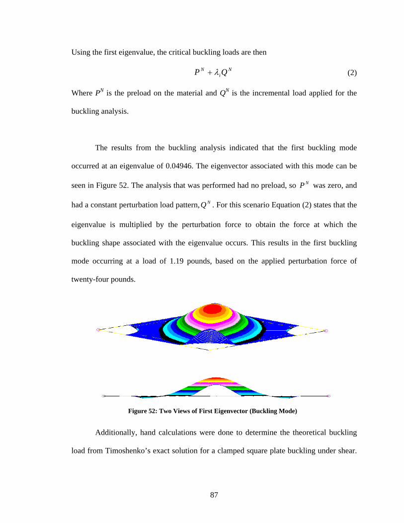
Using the first eigenvalue, the critical buckling loads are then
Ni
N QP λ+ (2)
Where PN is the preload on the material and QN is the incremental load applied for the
buckling analysis.
The results from the buckling analysis indicated that the first buckling mode
occurred at an eigenvalue of 0.04946. The eigenvector associated with this mode can be
seen in Figure 52. The analysis that was performed had no preload, so NP was zero, and
had a constant perturbation load pattern, NQ . For this scenario Equation (2) states that the
eigenvalue is multiplied by the perturbation force to obtain the force at which the
buckling shape associated with the eigenvalue occurs. This results in the first buckling
mode occurring at a load of 1.19 pounds, based on the applied perturbation force of
twenty-four pounds.
Additionally, hand calculations were done to determine the theoretical buckling
load from Timoshenko’s exact solution for a clamped square plate buckling under shear.
Figure 52: Two Views of First Eigenvector (Buckling Mode)
88
The following derivation can be found in its full form in Theory of Elastic Stability by
Timoshenko and Gere [1961].
First, it is assumed that the plate buckles in two half-waves, one representing the
deflection along each pair of parallel sides. With this assumption the total deflection can
be represented by the following equation:
by
axaw ππ sin2sin21= (3)
Expanding the assumption so that the out-of-plane deformation can be represented
by multiple half waves in each direction leads to
byn
axmaw mnmn
ππ sinsin= (4)
This is similar to expanding a Taylor series. To get the actual deflection one must sum
Equation 4 over a significantly large range of m and n. Therefore the total deflection is
written as
∑ ∑∞=
=
∞=
=
=m
m
n
nmn b
yna
xmaw1 1
sinsin ππ (5)
From this equation one can determine that the strain energy of bending will be
∑∑∞=
=
∞=
=⎟⎟⎠
⎞⎜⎜⎝
⎛+=∆
m
m
n
nmn b
namaabDU
1 1
2
2
2
2
22
4
42π (6)
89
Next the equation for the work done by external forces is found to be
∫ ∫ ∂∂
∂∂
−=∆a b
xy dxdyyw
xwNT
0 0
(7)
Substituting Equation (5) into Equation (7) gives two results in integral form, one
for m ± p being an even number, and the other for m ± p being an odd number. When
these are solved we obtain
( )( )∑∑∑∑ −−−=∆
m n p qpqmnxy nqpm
mnpqaaNT 22224 (8)
Equating the work from external forces (Equation (8)) and the strain energy of the system
(Equation (6)) we obtain an equation for determining the critical value of the shearing
forces seen in Equation (9).
( )( )∑∑∑∑
∑ ∑
−−
⎟⎟⎠
⎞⎜⎜⎝
⎛+
−=
∞=
=
∞=
=
m n p qpqmn
m
m
n
nmn
xy
nqpmmnpqaa
bn
ama
abDN
2222
1 1
2
2
22
2
222
32
ππ
(9)
The critical shear force is that which occurs when Equation (9) is at its minimum.
To determine this point one must take the derivative of Equation (9) with respect to each
of the coefficients and set them equal to zero. This provides a system of linear equations
than can be divided into two groups: equations with constants amn where m + n are odd
numbers, and one for which m + n are even numbers. For square plates both sets of
equations are needed, resulting in mn equations. As more of the equations are used the
results become more accurate. Using five equations and setting their determinant equal to
90
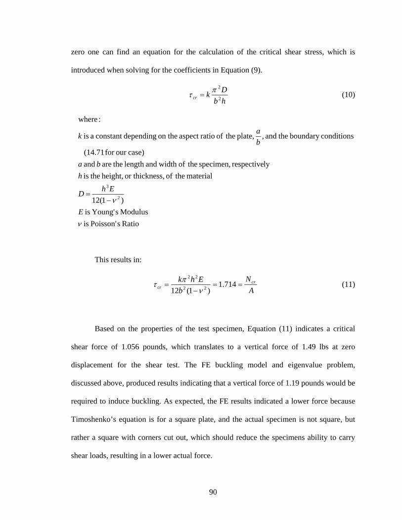
zero one can find an equation for the calculation of the critical shear stress, which is
introduced when solving for the coefficients in Equation (9).
hbDkcr 2
2πτ = (10)
Ratio sPoisson' is Modulus sYoung' is )1(12
material theof ss,or thickne height, theis lyrespective specimen, theof width andlength theare and
case)our for (14.71
conditionsboundary theand , plate, theof ratioaspect on the dependingconstant a is
:where
2
3
ν
νE
EhD
hba
bak
−=
This results in:
AN
bEhk cr
cr ==−
= 714.1)1(12 22
22
νπτ (11)
Based on the properties of the test specimen, Equation (11) indicates a critical
shear force of 1.056 pounds, which translates to a vertical force of 1.49 lbs at zero
displacement for the shear test. The FE buckling model and eigenvalue problem,
discussed above, produced results indicating that a vertical force of 1.19 pounds would be
required to induce buckling. As expected, the FE results indicated a lower force because
Timoshenko’s equation is for a square plate, and the actual specimen is not square, but
rather a square with corners cut out, which should reduce the specimens ability to carry
shear loads, resulting in a lower actual force.
91
Taking this data back to the model an analysis was run to determine at what force
and displacement the out-of-plane deformation first occurs. This was done by reviewing
results showing that the deformation occurred before 0.2 inch displacement. The analysis
was run to that displacement, with a small initial step size, and reaction forces requested
at each step.
The results were reviewed to see at which step the out-of-plane deformation was
first visible. The displacement at this step was 0.112 inches, which occurs only six
seconds into the minute long straining of the material. The resultant force at this step was
looked up, and found to be 1.42 pounds. The step before the displacement was noticed is
at 0.08 inch displacement, with a force of 0.72 pounds. So the deformation is first noticed
in the model at a step that has a load slightly above the predicted buckling load, which
indicates that buckling had just occurred. This means that the out-of-plane deformation
that is witnessed during the testing is buckling, not membrane folding.
The same model was run again, with the same initial time step, but a maximum
time step of 0.1, which requires that there would be a minimum of 10 data points. The
resulting 13 data points were broken into the resultant force and the “z”, or out-of-plane,
displacement and plotted against the “y” displacement of the specimen in Figure 53. This
plot is shown with the “z” displacement on the primary axis and the force on the
secondary axis. The horizontal red line indicates a force of 1.19 lbs, which occurs at
approximately 0.09 inches of displacement in the “y” direction.
92
From the plot it is easily seen that the force increases at a nearly constant rate
through the buckle, while the “z” displacement increases significantly after the bucking
has occurred. Visually this states that once the SMP buckles, it simply continues to fold
in the shape of the first buckling mode as it continues to be compressed in the first mode,
and not progress to other eigenvectors. This is believed to be stable buckling – when
there is no distinct ‘snap through’ of the material. Figure 54 shows a cooled specimen
after being tested to the full displacement. When compared to Figure 52 (or the top of
Figure 55), one can see that the first mode shape has been compressed, with larger out-of-
plane displacements resulting and that the specimen has not snapped to the next mode
shape with the continued application of force, which would be characteristic of unstable
buckling. The first and second mode shapes, or eignvectors, are compared in Figure 55.
0.00
0.02
0.04
0.06
0.08
0.10
0.12
0.14
0.16
0 0.02 0.04 0.06 0.08 0.1 0.12 0.14 0.16 0.18 0.2
"Y" Displacement [inches]
"Z"
Dis
plac
emen
t [in
ches
]
0
0.5
1
1.5
2
2.5
3
Forc
e (lb
s)
"z" Disp Force
Figure 53: Force and Displacement Data from Model
93
Stable buckling is so named because once the system has deformed it can still be
in equilibrium in its deformed position; it is just not the exact same shape as before the
buckling occurred. Essentially the equilibrium equation is continuous, and it’s first
derivative is positive, over an appropriately large enough range when plotted on a force-
displacement graph. Unstable buckling would occur if there were multiple stable
buckling curves for the equilibrium equation, and at least one unstable curve (when the
derivative is negative) that intersects multiple stable curves at their critical force. When
the load along one of the stable curves reaches its critical value, the structure will buckle
from one stable mode to another nearly instantly, and with a noticeable change in force.
Figure 54: Folded Specimen
Figure 55: First (top) and Second (bottom) Mode Shapes Seen Together
94
Since, for the case presented here, there is no distinct change in slope of the force, and the
buckling deformation appears smooth this cannot be unstable buckling [Hjelmstad,
1997].
5.3 Chapter Summary
This chapter established that it is possible to model shape memory polymers with
a finite element model, but only for small strain situations where the material strain
mechanism is nearly elastic. Under high strains the strain mechanism is more
complicated, and is therefore harder to model. The modeling was able to verify that the
out-of-plane deformation noted in the testing is in fact buckling. It was possible to verify
the fidelity of the model through comparison of shear stress-shear strain curves, and by
noting at what applied force and displacement the buckling occurred at during the testing.
95
CHAPTER VI
CONCLUSIONS
This final chapter provides a brief summary of the thesis and the conclusions that
were obtained from the research. This includes potential future work that can be used to
expand on the data presented here, and items to pursue to more fully model the
phenomena occurring in the SMPs during these tests.
6.1: Thesis Summary
This thesis began with an introduction to morphing aircraft and their inherent
advantages over current designs, including some current aircraft that exhibit a shape
change on a very small scale that improves their efficiency, speed, and range. A review of
some shape control concepts illustrated the types of shape control required. These
program descriptions focused specifically on their use of different technologies to
provide the flexible skin needed to achieve the project goals. The oldest program, the F-
111 Mission Adaptive Wing, used new technology of the time, with engineered fiberglass
skins to flex where needed. The two newer programs used elastomers attached nearly
continuously along actuators producing small deformations (Smart Wing) and a
reinforced elastomer actuated by a shape memory alloy (SAMPSON.) Key technologies
to enable these morphing aircraft in the near future include distributed, high power
96
density actuators, mechanized structures, and flexible skins. To allow for flexible skins
there are many technologies available, including a scaled skin (i.e. like a fish), sliding
skin panels, or making the skin out of elastomers or shape memory polymers, though
recent trends have been leaning away from scales and sliding panels due to their added
complication and hardware requirements.
The procedures used during the experimental process were described so they
could be repeated in the future, should one have access to the same equipment and
materials. This includes the environmental box that was designed to bring the test
specimen up to temperature and maintain the desired temperature throughout the test.
Also, a unique test fixture was needed to induce pure shear, from a tensile machine, over
a large range of shear strain. Chapter four provided the results of the experiments, and a
description of the material reactions to the experiments, ending with a brief list of
material properties.
Finally, a description of the modeling is provided. This includes the geometry,
elements, mesh, boundary conditions and constants for the initial models, and the
variations in mesh refinement, and modulus distribution with the use of temperature
dependent properties, that followed with each improvement to the model.
This research produced a number of ‘firsts’ in SMP testing. A shear fixture was
designed and manufactured to test shear in a tensile machine over extremely large
deformations, with shear strain up to and over 150%. A CRG employee who visited to
97
watch some of the testing indicated that it was the first time anyone at the company had
seen such a large amount of SMP strained so much (a 5” x 5” specimen strained 60%,) all
other tests witnessed by CRG employees were conducted on much smaller size
specimens (1” x 0.5”.)
The tensile tests were the first known testing of this SMP to specifically
determine the modulus at temperature. Previous testing was done with a Dynamic
Mechanical Analysis machine with one specimen tested continually over a range of
temperatures.
The procedures used were often modifications from some of the references,
helping push towards a core standard for testing shape memory polymers, which is
crucial to expanding use of the material and for properly classifying different formulas.
Finally, this research provided a solid base for further SMP testing and expanding
capabilities for modeling SMP behavior.
6.2: Conclusions & Recommendations
Based on the research conducted and the results obtained, shape memory
polymers remain a strong candidate material for skins on a morphing aircraft. There are
still some hurdles to clear with this young technology before it will be able to be used for
a full scale, large deformation aircraft, but many of the needed advancements are already
being researched.
98
To assist in the carrying of aerodynamic loads when above the Tg without
deforming there should be some form of reinforcement added to the material. In addition
to allowing higher pressures, this could have the added benefit of hindering the buckling
that was witnessed during testing. Additionally, prestrain should continue to be
investigated, including bi-axial prestrain. It is now known that it has an effect on the
buckling, but complete control of the buckling was not realized during this research,
though it appears to be possible. Finally, by advancing light activated SMPs and moving
away from thermally activated SMPs any effects of thermal expansion will be negated.
As was noted earlier the shear fixture increased the stress on the material at the
edge of the fixture. Creating a new design that does not do this would improve the
experiment by allowing a greater range of tests to be performed without premature
material failure. Also, with a larger supply of material more tests could be performed.
This is especially needed for prestrained specimens and for the tensile tests, as these two
tests lead to a better understanding of minimizing the buckling that occurs and providing
a more complete understanding of the strain mechanism seen in the material.
The analytical solution, while proven to have high fidelity at low strains, requires
more information from testing in order to provide accurate results at higher strains. Once
the strain mechanism is fully understood constants can be calculated to input into the
model to produce better results at high strains, and thus fully model the SMP during the
shear test.
99
APPENDIX A
Geometric Relations Used to Calculate Shear Stress
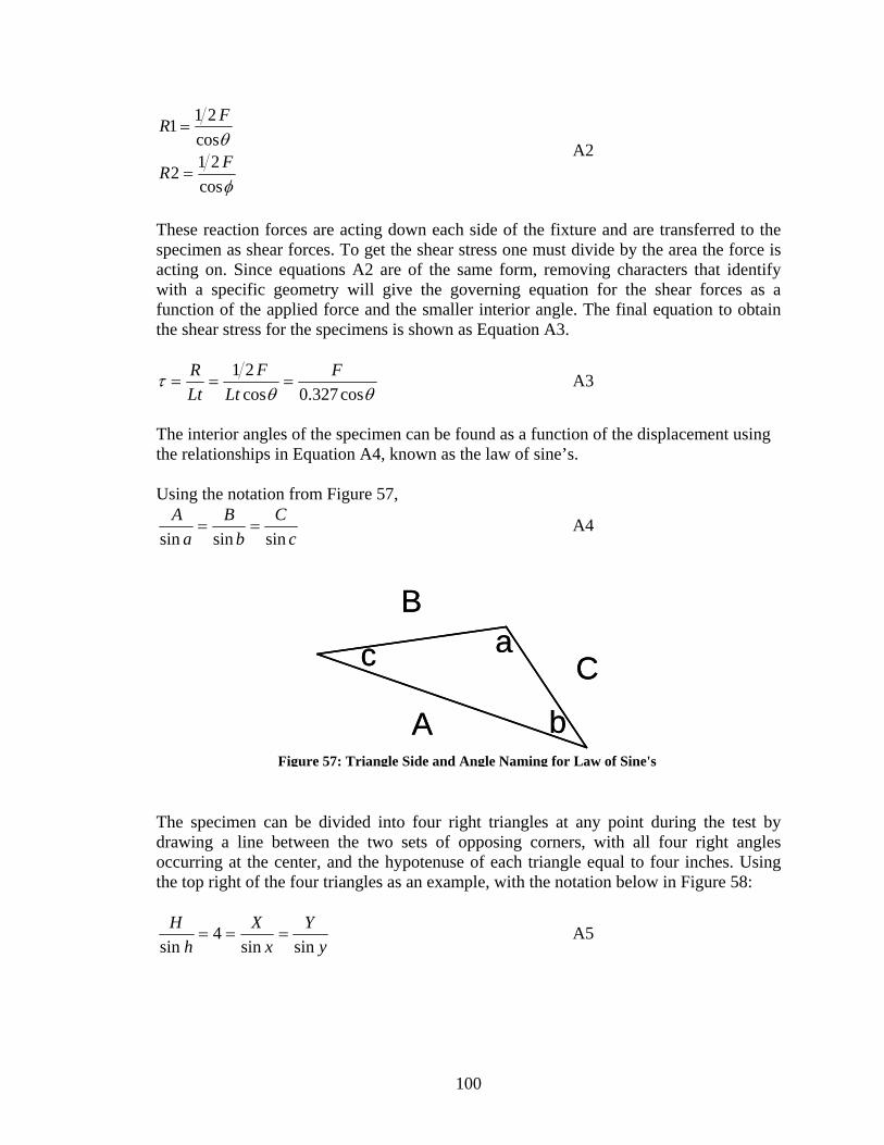
In Figure 56 above, with equivalent forces acting on the two different geometries the vertical components of each reaction, R1y and R2y, must be the same, ½ F.
yRFRyRFR221cos*2
121cos*1====
φθ
A1
With differing angles φ and θ, the resultants will be different, and can be found by rearranging equations A1 and solving for R1y and R2y.
F
R1θ
F
R2
φ
Figure 56: Reaction Forces & Geometry
100
φ
θ
cos212
cos211
FR
FR
=
= A2
These reaction forces are acting down each side of the fixture and are transferred to the specimen as shear forces. To get the shear stress one must divide by the area the force is acting on. Since equations A2 are of the same form, removing characters that identify with a specific geometry will give the governing equation for the shear forces as a function of the applied force and the smaller interior angle. The final equation to obtain the shear stress for the specimens is shown as Equation A3.
θθτ
cos327.0cos21 F
LtF
LtR
=== A3
The interior angles of the specimen can be found as a function of the displacement using the relationships in Equation A4, known as the law of sine’s. Using the notation from Figure 57,
cC
bB
aA
sinsinsin== A4
The specimen can be divided into four right triangles at any point during the test by drawing a line between the two sets of opposing corners, with all four right angles occurring at the center, and the hypotenuse of each triangle equal to four inches. Using the top right of the four triangles as an example, with the notation below in Figure 58:
yY
xX
hH
sinsin4
sin=== A5
A
B
Cc
b
a
A
B
Cc
b
a
Figure 57: Triangle Side and Angle Naming for Law of Sine's
101
The value for Y is simply the one half of the initial height of the specimen (corner to corner), plus the displacement, stated mathematically in A6. Where l0 is the initial height ( sqrt(32) = 5.65) and l∆ is the displacement.
20 ll
Y∆+
= A6
With two of the interior angles known, it is simple to find the third. Combining all of the above, the interior angle θ is found from Equation A7.
⎟⎟⎠
⎞⎜⎜⎝
⎛⎟⎠⎞
⎜⎝⎛ ∆+
−=
⎟⎟⎟⎟
⎠
⎞
⎜⎜⎜⎜
⎝
⎛
⎟⎟⎟⎟
⎠
⎞
⎜⎜⎜⎜
⎝
⎛ ∆+
−=
⎟⎟⎠
⎞⎜⎜⎝
⎛⎟⎠⎞
⎜⎝⎛−=−−==
−−
−
8sin902
42sin902
4sin902)90180(22
01
0
1
1
llll
Yyxθ
A7
Now the shear stress can be calculated as a function of the applied force and the displacement of the specimen.
H=4
h=90°
X
Y
x
y
H=4
h=90°
X
Y
x
y
Figure 58: Law of Sine's Definitions for Test Specimen
102
APPENDIX B
Shear Data
This appendix contains the plots of each individual shear test, with notable events pointed out under the respective plot.
0
20
40
60
80
100
120
0% 50% 100% 150% 200%
Percent Shear Strain [in/in]
Shea
r Stre
ss [p
si]
Figure 59: Sample #1 Test1 Note the increase in shear stress (applied force required to hold a position) when the specimen was cooled and held in a particular shape, at the maximum shear strain.
103
Material is pinched by the fixture at strains above 100% shear strain, this can be more readily seen by comparing to the plot for Sample #1Test4.
0
50
100
150
200
250
0% 50% 100% 150% 200%Percent Shear Strain [in/in]
Shea
r Stre
ss [p
si]
-20
0
20
40
60
80
100
120
0% 20% 40% 60% 80% 100% 120% 140% 160% 180%
Percent Shear Strain [in/in]
Shea
r Str
ess
[psi
]
pull 1 pull 2 pull 3 pull 4
Figure 60: Sample #1 Test2
Figure 61: Sample #1 Test3
104
Note a significantly larger shear stress above 100% shear strain, when compared to most other plots. This is from the material getting pinched by the fixture.
0
50
100
150
200
250
300
350
400
450
500
0% 1% 2% 3% 4% 5% 6%Percent Shear Strain [in/in]
Shea
r Stre
ss [p
si]
Figure 63: Sample #1 Cold Test
Note the change in shear stress just above 1% shear strain where specimen slipped.
0
50
100
150
200
250
300
350
400
450
0% 20% 40% 60% 80% 100% 120% 140% 160% 180%
Percent Shear Strain [in/in]
She
ar S
tress
[psi
]
pull 1 pull 2 pull 3 pull 4
Figure 62: Sample #1 Test4
105
-20
0
20
40
60
80
100
0% 20% 40% 60% 80% 100% 120% 140% 160% 180%
Percent Shear Strain [in/in]
Shea
r Str
ess
[psi
]
First pull Second Pull Third Pull Fourth Pull
-20
0
20
40
60
80
100
0% 20% 40% 60% 80% 100% 120% 140% 160% 180%
Percent Shear Strain [in/in]
Shea
r Str
ess
[psi
]
First pull Second Pull Third Pull Fourth Pull
Figure 65: Sample #2 Test3
Figure 64: Sample #2 Test2
106
Specimen pinched by fixture above 100% shear strain.
Figure 75: Sample #5 Test4 Cold deformation of the material reached the preset deformation limit of 1.0”. The material shows yielding, but no fracture, in cold shear tensile tests.