Image and Signal Processing with Non-Gaussian Noise: EM-Type

University of California

Los Angeles

Image and Signal Processing with Non-Gaussian Noise:

EM-Type Algorithms and Adaptive Outlier Pursuit

A dissertation submitted in partial satisfaction

of the requirements for the degree

Doctor of Philosophy in Mathematics

by

Ming Yan

2012

c© Copyright by

Ming Yan

2012

Abstract of the Dissertation

Image and Signal Processing with Non-Gaussian Noise:

EM-Type Algorithms and Adaptive Outlier Pursuit

by

Ming Yan

Doctor of Philosophy in Mathematics

University of California, Los Angeles, 2012

Professor Luminita A. Vese, Chair

Most of the studies of noise-induced phenomena assume that the noise source is Gaussian

because of the possibility of obtaining some analytical results when working with Gaussian

noises. The use of non-Gaussian noises is rare, mainly because of the difficulties in handling

them. However, there is experimental evidence indicating that in many phenomena, the noise

sources could be non-Gaussian, for example Poisson data and sparsely corrupted data. This

thesis provides two classes of algorithms for dealing with some special types of non-Gaussian

noise.

Obtaining high quality images is very important in many areas of applied sciences, and

the first part of this thesis is on expectation maximization (EM)-Type algorithms for im-

age reconstruction with Poisson noise and weighted Gaussian noise. In these two chapters,

we proposed general robust expectation maximization (EM)-Type algorithms for image re-

construction when the measured data is corrupted by Poisson noise and weighted Gaussian

noise, without and with background emission. This method is separated into two steps:

EM step and regularization step. In order to overcome the contrast reduction introduced by

some regularizations, we suggested EM-Type algorithms with Bregman iteration by applying

a sequence of modified EM-Type algorithms. One algorithm with total variation being the

regularization is used for image reconstruction in computed tomography application.

The second part of this thesis is on adaptive outlier pursuit method for sparsely corrupted

ii

data. In many real world applications, there are all kinds of errors in the measurements

during data acquisition and transmission. Some errors will damage the data seriously and

make the obtained data containing no information about the true signal, for example, sign

flips in measurements for 1-bit compressive sensing and impulse noise in images. Adaptive

outlier pursuit is used to detect the outlier and reconstruct the image or signal by iteratively

reconstructing the image or signal and adaptively pursuing the outlier. Adaptive outlier

pursuit method is used for robust 1-bit compressive sensing and impulse noise removal in

chapters 4 and 5 respectively.

iii

The dissertation of Ming Yan is approved.

Alex Bui

Jason Cong

Stanley Osher

Lieven Vandenberghe

Luminita A. Vese, Committee Chair

University of California, Los Angeles

2012

iv

To my family

for their constant source of

love, concern, support and strength all these years.

v

Table of Contents

1 Introduction . . . . . . . . . . . . . . . . . . . . . . . . . . . . . . . . . . . . . . 1

I EM-Type Algorithms 4

2 General Convergent Expectation Maximization (EM)-Type Algorithms for

Image Reconstruction Without Background Emission . . . . . . . . . . . . . 5

2.1 Introduction . . . . . . . . . . . . . . . . . . . . . . . . . . . . . . . . . . . . 5

2.2 Uniqueness of Solutions to Problems (2.5) and (2.7) . . . . . . . . . . . . . . 8

2.3 Expectation Maximization (EM) Iteration . . . . . . . . . . . . . . . . . . . 10

2.4 EM-Type Algorithms for Poisson data . . . . . . . . . . . . . . . . . . . . . 12

2.4.1 Equivalence to EM Algorithms with a priori Information . . . . . . . 14

2.4.2 Convergence of EM-Type Algorithms . . . . . . . . . . . . . . . . . . 15

2.4.3 EM-Type Algorithms are Alternating Minimization Methods . . . . . 18

2.5 Simultaneous Algebraic Reconstruction Technique (SART) is EM . . . . . . 20

2.6 EM-Type Algorithms for Gaussian Noise . . . . . . . . . . . . . . . . . . . . 21

2.6.1 Convergence Analysis of EM-Type Algorithms for Gaussian Noise . . 23


2.6.3 Relaxation . . . . . . . . . . . . . . . . . . . . . . . . . . . . . . . . . 27

2.7 Numerical Experiments . . . . . . . . . . . . . . . . . . . . . . . . . . . . . . 29

2.7.1 CT Reconstruction by EM-TV (2D) . . . . . . . . . . . . . . . . . . . 30

2.7.2 Reconstruction using EM-MSTV (2D) . . . . . . . . . . . . . . . . . 33

2.7.3 Reconstruction using EM-TV (3D) . . . . . . . . . . . . . . . . . . . 33

2.8 Conclusion . . . . . . . . . . . . . . . . . . . . . . . . . . . . . . . . . . . . . 33

vi

3 General Convergent EM-Type Algorithms for Image Reconstruction With

Background Emission and Poisson Noise . . . . . . . . . . . . . . . . . . . . . . 36

3.1 Introduction . . . . . . . . . . . . . . . . . . . . . . . . . . . . . . . . . . . . 36

3.2 Expectation Maximization (EM) Iteration . . . . . . . . . . . . . . . . . . . 38

3.3 EM-Type Algorithms for Image Reconstruction . . . . . . . . . . . . . . . . 40

3.3.1 Equivalence to EM Algorithms with a priori Information . . . . . . . 42

3.3.2 Convergence of EM-Type Algorithms . . . . . . . . . . . . . . . . . . 43


3.3.4 Further Analysis for the Case Without Regularization . . . . . . . . . 48

3.4 EM-Type Algorithms with Bregman Iteration . . . . . . . . . . . . . . . . . 50

3.5 Numerical Experiments . . . . . . . . . . . . . . . . . . . . . . . . . . . . . . 51

3.6 Conclusion . . . . . . . . . . . . . . . . . . . . . . . . . . . . . . . . . . . . . 58

II Adaptive Outlier Pursuit 60

4 Adaptive Outlier Pursuit for Robust 1-Bit Compressive Sensing . . . . . 61

4.1 Introduction . . . . . . . . . . . . . . . . . . . . . . . . . . . . . . . . . . . . 61

4.2 Robust 1-bit Compressive Sensing using

Adaptive Outlier Pursuit . . . . . . . . . . . . . . . . . . . . . . . . . . . . . 64

4.3 The case with L unknown . . . . . . . . . . . . . . . . . . . . . . . . . . . . 67

4.4 Numerical Results . . . . . . . . . . . . . . . . . . . . . . . . . . . . . . . . . 68

4.4.1 Noise levels test . . . . . . . . . . . . . . . . . . . . . . . . . . . . . . 69

4.4.2 M/N test . . . . . . . . . . . . . . . . . . . . . . . . . . . . . . . . . 71

4.4.3 High noise levels . . . . . . . . . . . . . . . . . . . . . . . . . . . . . 74

4.4.4 L mismatch . . . . . . . . . . . . . . . . . . . . . . . . . . . . . . . . 75

4.4.5 Unknown L . . . . . . . . . . . . . . . . . . . . . . . . . . . . . . . . 76

vii

4.5 Conclusion . . . . . . . . . . . . . . . . . . . . . . . . . . . . . . . . . . . . . 76

5 Impulse Noise Removal . . . . . . . . . . . . . . . . . . . . . . . . . . . . . . . 79

5.1 Introduction . . . . . . . . . . . . . . . . . . . . . . . . . . . . . . . . . . . . 79

5.2 The Adaptive Center-Weighted Median Filter . . . . . . . . . . . . . . . . . 82

5.3 Blind Inpainting Models using ℓ0 Norm . . . . . . . . . . . . . . . . . . . . . 84

5.3.1 Formulation . . . . . . . . . . . . . . . . . . . . . . . . . . . . . . . . 84

5.3.2 Algorithm . . . . . . . . . . . . . . . . . . . . . . . . . . . . . . . . . 85

5.3.3 TV Blind Inpainting . . . . . . . . . . . . . . . . . . . . . . . . . . . 86

5.4 Blind Inpainting Using Adaptive Outlier Pursuit . . . . . . . . . . . . . . . . 87

5.4.1 Framelet-Based Deblurring . . . . . . . . . . . . . . . . . . . . . . . 89

5.5 Convergence Analysis . . . . . . . . . . . . . . . . . . . . . . . . . . . . . . . 91

5.6 Experiments . . . . . . . . . . . . . . . . . . . . . . . . . . . . . . . . . . . . 95

5.7 Conclusion . . . . . . . . . . . . . . . . . . . . . . . . . . . . . . . . . . . . . 103

References . . . . . . . . . . . . . . . . . . . . . . . . . . . . . . . . . . . . . . . . . 107

viii

List of Figures

2.1 2D Shepp-Logan phantom . . . . . . . . . . . . . . . . . . . . . . . . . . . . 30

2.2 Top from left to right: reconstruction result in the noise-free case using FBP

with 36, 180 and 360 views, and result using EM-TV with 36 views. Bottom

from left to right: reconstruction result in the noisy case using FBP with 36,

180 and 360 views, and result using EM-TV with 36 views. The root mean

square errors are also given. . . . . . . . . . . . . . . . . . . . . . . . . . . . 32

2.3 Comparisons of TV regularization and MSTV regularization for both without

and with noise cases. Top row shows the reconstructed images by these two

methods in both cases, Bottom row shows the differences between the recon-

structed images and original phantom image. The RMSEs and differences

show that MSTV can provide better results than TV only. . . . . . . . . . . 34

2.4 Reconstruction results in three dimensions for the noise-free case. First col-

umn: two-dimensional views of the original three-dimensional Shepp-Logan

phantom. Middle column: two-dimensional views of reconstruction results

obtained using EM-TV algorithm. Last column: two-dimensional views of

reconstruction results obtained using EM iteration. The root mean square

errors are also given. . . . . . . . . . . . . . . . . . . . . . . . . . . . . . . . 35

3.1 (a) The orginal image u∗. (b) Blurred image K ∗ u∗ using a Gaussian blur

kernel K. (c) The deblurred image using the proposed EM-TV with Bregman

iteration. (d) The difference between the deblurred image and the original

image. (e) The lineouts of original image, blurred image and deblurred image

in the middle row. Some parameters chosen are β = 5, Num inner = 1 and

Num outer = 10000. . . . . . . . . . . . . . . . . . . . . . . . . . . . . . . . 52

ix

3.2 (a) The result without Bregman iteration. (b) The result with 25 Bregman

iterations. (c) The result with 100 Bregman iterations. (d) The plot of RMSE

versus Bregman iterations. (e) The lineouts of original image, blurred image,

the results with and without Bregman iterations. Some parameters chosen

are β = 0.001, Num inner = 100 and Num outer = 100. . . . . . . . . . . . . 53

3.3 (a) The noisy blurred image. (b) The result without Bregman iteration. (c)

The result with 9 Bregman iterations. (d) The plot of KL distances versus

Bregman iterations. (e) The lineouts of original image, blurred image, the

results with and without Bregman iterations. Some parameters chosen are

β = 1, Num inner = 200 and Num outer = 15. . . . . . . . . . . . . . . . . . 54

3.4 (a) The original image. (b) The PSF image. (c) The blurred image. (d) The

noisy blurred image. (e) Initial guess from CG. (f) The result of EM-Type

algorithm with Bregman iterations. (g) The plot of KL versus Bregman iter-

ations. (h) The RMSE versus Bregman iterations. Some parameters chosen

are β = 1, Num inner = 200 and Num outer = 30. . . . . . . . . . . . . . . . 56

3.5 (a) The original image. (b) The PSF image. (c) The blurred image. (d) The

noisy blurred image. (e) Initial guess from HyBR. (f) The result of EM-Type

algorithm with Bregman iterations. (g) The plot of KL versus Bregman iter-

ations. (h) The RMSE versus Bregman iterations. Some parameters chosen

are β = 10−5, Num inner = 10 and Num outer = 250. . . . . . . . . . . . . . 57

3.6 Top row shows raw lensfree fluorescent images of different pairs of particles.

The distances betweens thes two particles are 30µm, 21µm, 18µm, 13µm and

9µm, from left to right. Middle row shows the results of EM-Type algorithm

with p = 0.5. Bottom row shows the results for EM (or Richardson-Lucy)

method. . . . . . . . . . . . . . . . . . . . . . . . . . . . . . . . . . . . . . . 58

x

4.1 Algorithm comparison on corrupted data with different noise levels. (a) av-

erage SNR versus noise level, (b) average angular error versus noise level, (c)

average Hamming error between A(x) and A(x∗) versus noise level, (d) aver-

age Hamming distance between A(x) and noisy measurements y versus noise

level. AOP proves to be more robust to measurement sign flips compared with

BIHT. . . . . . . . . . . . . . . . . . . . . . . . . . . . . . . . . . . . . . . . 70

4.2 The probabilities of correct detections of sign flips for different noise levels

ranging from 0.5% to 10%. AOP and AOP-f have very high accuracy (great

than 90%) in detecting the sign flips, while AOP-ℓ2 and AOP-ℓ2-f have rela-

tively lower accuracy (around 80%). . . . . . . . . . . . . . . . . . . . . . . . 71

4.3 Algorithm comparison on corrupted data with different M/N . (a) average

SNR versus M/N , (b) average angular error versus M/N , (c) average Ham-

ming error between A(x) and A(x∗) versus M/N , (d) average Hamming dis-

tance between A(x) and y versus M/N , (e) average percentage of coefficient

misses versus M/N . AOP yields a remarkable improvement in reducing the

Hamming and angular error and achieving higher SNR. . . . . . . . . . . . . 72

4.4 Hamming error versus angular error with different M ’s. AOP gives the most

consistent results for M = 0.7N and M = 1.5N . In these two cases we can

see a linear relationship ǫsim ≈ C + ǫH between the average angular error

ǫsim and average Hamming error ǫH , where C is a constant. For really small

M (M = 0.1N) BIHT returns almost the same results as AOP as AOP may

fail to find the exact sign flips in the noisy measurements. The dashed line

ǫ1000 + ǫH is an upper bound for 1000 trials. . . . . . . . . . . . . . . . . . . 73

xi

4.5 The performance of AOP and AOP-ℓ2 under different noise levels. (a) average

angular error versus M/N with different noise levels, (b) correct detection

percentage versus M/N with different noise levels, (c) average angular error

versus K with different noise levels, (d) correct detection percentage versus

K with different noise levels. The performance gets better when we increase

M/N or decrease K. . . . . . . . . . . . . . . . . . . . . . . . . . . . . . . . 75

4.6 The performance of AOP with different L inputs. L has to stay close to its

true value in order to get good performance. . . . . . . . . . . . . . . . . . . 76

4.7 Comparison of results by different L’s at different noise levels from 1% to 10%.

(a) average angular error versus noise level, (b) average Hamming distance

between A(x) and noisy y versus noise level. By choosing appropriate L as

the input, we can obtain the results comparable to those with exact L. . . . 77

5.1 Noisy images and the sets detected by ACWMF. Left column: noisy images

corrupted by random-valued impulse noise; Right column: the sets of damaged

pixels detected by ACWMF. White point means that the corresponding pixel

is corrupted by impulse noise. . . . . . . . . . . . . . . . . . . . . . . . . . . 83

5.2 Denoising results of images contaminated by both Gaussian noise and salt-

and-pepper impulse noise with σ = 10 and s = 30%. Top row: noisy images;

Second row: the results restored by AMF; Third row: the results restored by

TVL1; Bottom row: the results restored by total variation blind inpainting

using AOP. . . . . . . . . . . . . . . . . . . . . . . . . . . . . . . . . . . . . 98

5.3 Denoising results of images contaminated by both Gaussian noise and random-

valued impulse noise with σ = 10 and s = 25%. Top row: noisy images;

Second row: the results restored by ACWMF; Third row: the results restored

by TVL1; Bottom row: the results restored by total variation blind inpainting

using AOP. . . . . . . . . . . . . . . . . . . . . . . . . . . . . . . . . . . . . 101

xii

5.4 The restored results of images blurred by fspecial(’disk’,3) and corrupted

by random-valued impulse noise (level s = 55%) at random set and Gaussian

noise (STD σ = 5). Top row: blurry and noisy images; Middle row: the results

restored by Fast IFASDA; Bottom row: the results restored Ada Fast IFASDA.103

5.5 The restored results of images blurred by fspecial(’disk’,3) and cor-

rupted by random-valued impulse noise (level s = 36.83%) at specific set

and Gaussian noise (STD σ = 5). Top row: blurry and noisy images; Middle

row: the results restored by Fast IFASDA; Bottom row: the results restored

Ada Fast IFASDA. . . . . . . . . . . . . . . . . . . . . . . . . . . . . . . . . 104

5.6 The damaged pixels detected by ACWMF and Ada IFASDA. Left column:

the set obtained by ACWMF; Right column: the set obtained by Ada IFASDA105

5.7 PSNR values for different K/|Λc| for cameraman image when the level of

random-valued impulse noise is 40%. . . . . . . . . . . . . . . . . . . . . . . 106

xiii

List of Tables

5.1 PSNR(dB) for denoising results of different algorithms for noisy images cor-

rupted by salt-and-pepper impulse noise and mixed Gaussian impulse noise.

σ is the standard deviation for the Gaussian noise and s is the level of salt-

and-pepper impulse noise. . . . . . . . . . . . . . . . . . . . . . . . . . . . . 97

5.2 PSNR(dB) for denoising results of different algorithms for noisy images cor-

rupted by random-valued impulse noise and mixed Gaussian impulse noise. σ

is the standard deviation for the Gaussian noise and s is the level of random-

valued impulse noise. . . . . . . . . . . . . . . . . . . . . . . . . . . . . . . . 99

5.3 PSNR(dB) and CPU computing time (seconds) for deblurred results of dif-

ferent algorithms for blurred images corrupted by random-valued impulse

noise plus Gaussian noise. The images are blurred by the blurring kernel

fspecial(’disk’,3). . . . . . . . . . . . . . . . . . . . . . . . . . . . . . . 102

xiv

Acknowledgments

Foremost, I would like to express my deep appreciation to my advisor Professor Luminita

A. Vese for her professional advice, dedicated guidance, constant support, collaboration and

insight. I learned not only numerous ideas and ways to conduct research, but also many

other things beyond academics.

Besides, I would like to thank Professor Alex Bui and Professor Jason Cong for their

stimulating discussion in the group meetings at CDSC (Center of Domain Specific Comput-

ing) and support for the last three years. I must absolutely thank Professor Stanley Osher

for organizing the level set collective every week. I also want to thank Professor Lieven

Vandenberghe for offering the optimization courses.

I am thankful to Professor Andrea Bertozz and Professor Joseph Teran for their help in

my studies and research. I also appreciate the helpful discussions and suggestions I received

from postdoctoral and graduate students in CDSC and the math department, which includes

Dr. Jianfeng Cai, Dr. Jianwen Chen, Dr. Bin Dong, Feng Guan, Dr. Rongjie Lai, Dr. Wenye

Ma, Xiaokui Yang, Yi Yang, Yi Zou and many others.

My gratitude further goes to my friends who made my graduate study colorful and

joyful. I am also thankful to all of the people who work in Department of Mathematics

and Department of Computer Science here at UCLA for all of their help, especially, Maggie

Albert, Martha Contreras, Babette Dalton and Alexandra Luong.

Finally, I would like to thank my parents and my younger sister in China, whom this

thesis is dedicated to.

The research presented in this dissertation was supported by NSF Grant DMS-0714945

and Center for Domain-Specific Computing (CDSC) under the NSF Expeditions in Com-

puting Award CCF-0926127.

xv

Vita

2005 B.S. (Computational Mathematics),

University of Science and Technology of China, P. R. China.

2008 M.S. (Computational Mathematics),

University of Science and Technology of China, P. R. China.

2008–2012 Teaching and Research Assistant, Department of Mathematics,

University of California, Los Angeles, California, USA.

Publications

M. Yan, Y. Yang and S. Osher, Robust 1-bit compressive sensing using adaptive outlier

pursuit, IEEE Transactions on Signal Processing, to appear.

J. Chen, J. Cong, M. Yan and Y. Zou, FPGA-accelerated 3D reconstruction using com-

pressive sensing, In: Proceedings of the ACM/SIGDA International Symposium on Field

Programmable Gate Arrays (FPGA 2012), 163-166.

M. Yan, EM-type algorithms for image reconstruction with background emission and

Poisson noise, In: Proceedings of 7th International Symposium on Visual Computing, Lecture

Notes in Computer Science (LNCS), 6938 (2011), 33-42.

M. Yan, J. Chen, L. A. Vese, J. Villasenor, A. Bui and J. Cong, EM+TV based recon-

struction for cone-beam CT with reduced radiation, In: Proceedings of 7th International

Symposium on Visual Computing, Lecture Notes in Computer Science (LNCS), 6938 (2011),

1-10.

xvi

J. Chen, M. Yan, L. A. Vese, J. Villasenor, A. Bui and J. Cong, EM+TV for recon-

struction of cone-beam CT with curved detectors using GPU, In: Proceedings of Interna-

tional Meeting on Fully Three-Dimensional Image Reconstruction in Radiology and Nuclear

Medicine, 2011, 363-366.

M. Yan and L. A. Vese, Expectation maximization and total variation based model for

computed tomography reconstruction from undersampled data, In: Proceedings of SPIE

Medical Imaging: Physics of Medical Imaging, 7961 (2011), 79612X. doi:10.1117/12.878238

H. Han and M. Yan, A mixed finite element method on a staggered mesh for Navier-Stokes

equations, Journal of Computational Mathematics, 26 (2008), 816-824.

H. Han, M. Yan and C. Wu, An energy regularization method for the backward diffu-

sion problem and its applications to image deblurring, Communications in Computational

Physics, 4 (2008), 177-194.

xvii

CHAPTER 1

Introduction

Most of the studies of noise-induced phenomena assume that the noise source is Gaussian

because of the possibility of obtaining some analytical results when working with Gaussian

noises. The use of non-Gaussian noises is rare, mainly because of the difficulties in han-

dling them. However, there is experimental evidence indicating that in many phenomena,

the noise sources could be non-Gaussian, for example Poisson data and sparsely corrupted

data. The methods for image and signal processing are different when different types of

non-Gaussian noise are considered. In this thesis, we provide two classes of algorithms: ex-

pectation maximization (EM)-Type algorithms for image reconstruction with Poisson and

weighted Gaussian noise, and adaptive outlier pursuit for image and signal reconstruction

with sparsely corrupted data.

Obtaining high quality images is very important in many areas of applied sciences, such

as medical imaging, optical microscopy and astronomy. The degradation model can be

formulated as a linear inverse and ill-posed problem:

y = Ax+ b+ n. (1.1)

Here x is the image to be reconstructed, A represents a model for the imaging device and

is assumed to be linear, b is the background emission, y is the measured data and n is the

non-Gaussian noise depending on Ax + b. The problem is to find x with A, b and y given.

We proposed EM-Type algorithms for solving this problem when the noise n is Poisson noise

and weighted Gaussian noise. These algorithms are performed by iteratively applying the

EM step and regularization step.

1

Chapter 2 deals with the case without background emission (b = 0). In this chapter

we proposed a class of EM-Type algorithms for image reconstruction with Poisson noise

and weighted Gaussian noise. We proved the convergence of these algorithms by showing

that the proposed EM-Type algorithms are equivalent to EM algorithms [1] with a priori

information and alternating minimization methods for equivalent optimization problems.

The performance of one algorithm with total variation (TV) [2] being the regularization,

named EM-TV, is shown for image reconstruction in a computed tomography application.

Chapter 3 considers the case with background emission (b 6= 0), which occurs in astron-

omy and fluorescence microscopy. Similarly, we proposed a class of EM-Type algorithms for

image reconstruction with Poisson noise and proved the convergence by showing the equiv-

alence of EM-Type algorithms, EM algorithms with a priori information and alternating

minimization methods for equivalent optimization problems. However, for some regular-

izations, the reconstructed images will lose contrast. To overcome this problem, EM-Type

algorithms with Bregman iteration are introduced. The performance of EM-Type algorithms

with or without Bregman iterations is shown for image deblurring.

The second part is on image and signal reconstruction with sparsely corrupted data. In

many real world applications such as signal and image processing, there are all kinds of errors

in the measurements during data acquisition and transmission. Some errors will damage the

data seriously and make the obtained data containing no information about the true signal.

Therefore, using this damaged data for signal reconstruction is useless and may worsen the

performance of reconstruction methods, and methods robust to these outliers are strongly

needed. For some applications like impulse noise removal, there are methods for detecting

the damaged pixels: adaptive median filter (AMF) [3] is used in salt-and-pepper impulse

noise removal and adaptive center wighted median filter (ACWMF) [4] is used in random-

valued impulse noise removal. But the performance of ACWMF is not good enough when

the number of pixels corrupted is very large. For other applications like 1-bit compressive

sensing [5], there are no methods for detecting the sign flips in the measurements. Adaptive

outlier pursuit is proposed to pursue the outliers adaptively by iteratively reconstructing the

image or signal and detect the outliers.

2

Chapter 4 applies the adaptive outlier pursuit on robust 1-bit compressive sensing (CS)

when some of the measurements are wrong. The classic compressive sensing (CS) theory

assumes the measurements to be real-valued and have infinite bit precision. The quantization

of CS measurements has been studied recently and it has been shown that accurate and

stable signal acquisition is possible even when each measurement is quantized to only one

single bit. The performance of all existing algorithms is worsened when there are a lot of

sign flips in the measurements. We propose a robust method for recovering signals from

1-bit measurements using adaptive outlier pursuit. This method will detect the positions

where sign flips happen and recover the signals using “correct” measurements. Numerical

experiments show the accuracy of sign flips detection and high performance of signal recovery

for our algorithms compared with other algorithms.

Chapter 5 is to solve the problem of image restoration of observed images corrupted by

impulse noise (and mixed Gaussian impulse noise). Since the pixels damaged by impulse noise

contain no information about the true image, how to find this set correctly is a very important

problem. We proposed two methods based on blind inpainting and ℓ0 minimization that can

simultaneously find the damaged pixels and restore the image. By iteratively restoring the

image and updating the set of damaged pixels, these methods have better performance than

other methods, as shown in the experiments. In addition, we provide convergence analysis

for these methods; these algorithms will converge to coordinatewise minimum points. In

addition, they will converge to local minimum points (with probability one) with some

modifications in the algorithms.

3

Part I

EM-Type Algorithms

4

CHAPTER 2

General Convergent Expectation Maximization

(EM)-Type Algorithms for Image Reconstruction

Without Background Emission

2.1 Introduction

Obtaining high quality images is very important in many areas of applied science, such as

medical imaging, optical microscopy and astronomy. For some applications such as positron-

emission-tomography (PET) and computed tomography (CT), analytical methods for im-

age reconstruction are available. For instance, filtered back projection (FBP) is the most

commonly used method for image reconstruction from CT by manufacturers of commercial

imaging equipments [6]. However, it is sensitive to noise and suffers from streak artifacts

(star artifacts). An alternative to this analytical reconstruction is the use of the iterative

reconstruction technique, which is quite different from FBP. The main advantages of the

iterative reconstruction technique over FBP are insensitivity to noise and flexibility [7]. The

data can be collected over any set of lines, the projections do not have to be distributed

uniformly in angle, and the projections can be even incomplete (limited angle). With the

help of parallel computing and graphics processing units (GPUs), even iterative methods can

be solved very fast. Therefore, iterative methods become more and more important, and we

will focus on the iterative reconstruction technique only.

The degradation model can be formulated as a linear inverse and ill-posed problem:

y = Ax+ b+ n. (2.1)

5

Here, y is the measured data (vector in RM for the discrete case). A is a compact operator

(matrix in RM×N for the discrete case). For all the applications we will consider, the entries

of A are nonnegative and A does not have full column rank. x is the desired exact image

(vector in RN for the discrete case). b is the background emission and n is the noise (both

are vectors in RM for the discrete case). We will consider the case without background

emission (b = 0) in this chapter. The case with background emission (b 6= 0) is considered

in the next chapter. Since the matrix A does not have full column rank, the computation

of x directly by finding the inverse of A is not reasonable because (2.1) is ill-posed and n is

unknown. Even for the case without noise (n = 0), there are many solutions because A does

not have full column rank. When there is noise in the measured data (n 6= 0), finding x is

more difficult because of the unknown n. Therefore regularization techniques are needed for

solving these problems efficiently.

One powerful technique for applying regularization is the Bayesian model, and a gen-

eral Bayesian model for image reconstruction was proposed by Geman and Geman [8], and

Grenander [9]. The idea is to use a priori information about the image x to be reconstructed.

In the Bayesian approach, we assume that measured data y is a realization of a multi-valued

random variable, denoted by Y and the image x is also considered as a realization of another

multi-valued random variable, denoted by X . Therefore the Bayesian formula gives us

pX(x|y) =pY (y|x)pX(x)

pY (y). (2.2)

This is a conditional probability of having X = x given that y is the measured data. After

inserting the detected value of y, we obtain a posteriori probability distribution of X . Then

we can find x∗ such that pX(x|y) is maximized, as maximum a posteriori (MAP) likelihood

estimation.

In general, X is assigned as a Gibbs random field, which is a random variable with the

following probability distribution

pX(x) ∼ e−βJ(x), (2.3)

6

where J(x) is a given convex energy functional, and β is a positive parameter. There are many

different choices for J(x) depending on the applications. Some examples are, for instance,

quadratic penalization J(x) = ‖x‖22/2 [10, 11], quadratic Laplacian J(x) = ‖∇x‖22/2 [12],

total variation J(x) = ‖|∇x|‖1 [13, 14, 15, 16, 17], and Good’s roughness penalization

J(x) = ‖|∇x|2/x‖1 [18], where ‖ · ‖1 and ‖ · ‖2 are the ℓ1 and ℓ2 norms respectively.

For the choices of probability densities pY (y|x), we can choose

pY (y|x) ∼ e−‖Ax−y‖22/(2σ2) (2.4)

in the case of additive Gaussian noise, and the minimization of the negative log-likelihood

function gives us the famous Tikhonov regularization method [19]

minimizex

1

2‖Ax− y‖22 + βJ(x). (2.5)

If the random variable Y of the detected values y follows a Poisson distribution [20, 21] with

an expectation value provided by Ax instead of Gaussian distribution, we have

yi ∼ Poisson(Ax)i, i.e., pY (y|x) ∼∏

i

(Ax)yiiyi!

e−(Ax)i . (2.6)

By minimizing the negative log-likelihood function, we obtain the following optimization

problem

minimizex≥0

∑

i

(

(Ax)i − yi log(Ax)i)

+ βJ(x). (2.7)

In this chapter, we will focus on solving (2.5) and (2.7). It is easy to see that the objective

functions in (2.5) and (2.7) are convex. Additionally, with suitably chosen regularization

J(x), the objective functions are strictly convex, and the solutions to these problems are

unique.

The work is organized as follows. The uniqueness of the solutions to problems (2.5) and

(2.7) are provided in section 2.2 for the discrete modeling. In section 2.3, we will give a short

introduction of expectation maximization (EM) iteration, or Richardson-Lucy algorithm,

7

used in image reconstruction without background emission from the view of optimization.

In section 2.4, we will propose general EM-Type algorithms for image reconstruction without

background emission when the measured data is corrupted by Poisson noise. This is based on

the maximum a posteriori likelihood estimation and an EM step. In this section, these EM-

Type algorithms are shown to be equivalent to EM algorithms with a priori information, and

their convergence is shown in two different ways. In addition, these EM-Type algorithms are

also considered as alternating minimization methods for equivalent optimization problems.

When the noise is weighted Gaussian noise, we also have the similar EM-Type algorithms.

Simultaneous algebraic reconstruction technique is shown to be EM algorithm in section 2.5,

and EM-Type algorithms for weighted Gaussian noise are introduced in section 2.6. In

section 2.6, we also show the convergence analysis of EM-Type algorithms for weighted

Gaussian noise via EM algorithms with a priori information and alternating minimization

methods. Some numerical experiments in CT reconstruction are given in section 2.7 to show

the efficiency of the EM-Type algorithms. We will end this work by a short conclusion

section.

2.2 Uniqueness of Solutions to Problems (2.5) and (2.7)

As mentioned in the introduction, the original problem without regularization is ill-posed.

Therefore at least one of these three properties: (i) a solution of the problem exists, (ii)

the solution is unique, and (iii) the solution depends continuously on the data, are not

fulfilled. For the well-posedness of the continuous modeling of problems (2.5) and (2.7),

the analysis will be different depending on different regularizations. If J(x) = ‖|∇x|‖1, i.e,.the regularization is the total variation, the well-posedness of the regularization problems

is shown in [22] and [15] for Gaussian and Poisson noise respectively. However, for discrete

modeling, the well-posedness of the problems is easy to show, because problems (2.5) and

(2.7) are convex. We have to just show that the solutions are unique.

In discrete modeling, the operator A is a matrix and x is a vector. After imposing some

reasonable assumptions on J(x) and A, the objective functions are strictly convex, therefore

8

the solutions are unique. The strict convexity means that given two different vectors x1 and

x2, then for any w ∈ (0, 1), the new vector xw = wx1 + (1− w)x2 satisfies

1

2‖Axw − y‖22 + βJ(xw) <w

1

2‖Ax1 − y‖22 + wβJ(x1)

+ (1− w)1

2‖Ax2 − y‖22 + (1− w)βJ(x2). (2.8)

If the objective function is not strictly convex, then we can find two different vectors x1 and

x2 and w ∈ (0, 1) such that

1

2‖Axw − y‖22 + βJ(xw) ≥w

1

2‖Ax1 − y‖22 + wβJ(x1)

+ (1− w)1

2‖Ax2 − y‖22 + (1− w)βJ(x2). (2.9)

From the convexity of the objective function, we have

1

2‖Axw − y‖22 + βJ(xw) =w

1

2‖Ax1 − y‖22 + wβJ(x1)

+ (1− w)1

2‖Ax2 − y‖22 + (1− w)βJ(x2), (2.10)

for all w ∈ (0, 1). Since 12‖Ax− y‖22 and J(x) are convex, we have

1

2‖Axw − y‖22 = w

1

2‖Ax1 − y‖22 + (1− w)

1

2‖Ax2 − y‖22, (2.11)

J(xw) = wJ(x1) + (1− w)J(x2), (2.12)

for all w ∈ (0, 1). From the equation (2.11), we have Ax1 = Ax2. If A is injective, i.e., the null

space of A is trivial, x1 and x2 have to be equal, then the objective function is strictly convex.

If A is not injective (A does not have full column rank), for instance, reconstruction from PET

and CT with undersampled data, we have to also consider equation (2.12). The equality

in (2.12) depends on the regularization J(x). For quadratic penalization, J(x) is strictly

convex, which implies x1 = x2, while for quadratic Laplacian, the equation (2.12) gives us

∇x1 = ∇x2. If J(x) is the total variation, we obtain, from the equality, that ∇x1 = α∇x2

9

with α ≥ 0 and depending on the pixel (or voxel). When Good’s roughness penalization

is used, we have ∇x1

x1 = ∇x2

x2 from the equality. Thus, if the matrix A is chosen such that

we can not find two different vectors (images) satisfying Ax1 = Ax2 and ∇x1 = α∇x2,

the objective function is strictly convex. Actually, this assumption is reasonable and in

the applications mentioned above, it is satisfied. Therefore, for the discrete modeling, the

optimization problem has a unique solution. If Poisson noise, instead of Gaussian noise,

is assumed, the objective function is still strictly convex, and the problem has a unique

solution.

2.3 Expectation Maximization (EM) Iteration

A maximum likelihood (ML) method for image reconstruction based on Poisson data was

introduced by Shepp and Vardi [21] in 1982 for image reconstruction in emission tomography.

In fact, this algorithm was originally proposed by Richardson [23] in 1972 and Lucy [24] in

1974 for image deblurring in astronomy. The ML method is a method for solving the special

case of problem (2.7) without regularization term, i.e., J(x) is a constant, which means

we do not have any a priori information about the image. From equation (2.6), for given

measured data y, we have a function of x, the likelihood of x, defined by pY (y|x). Then a

ML estimation of the unknown image is defined as any maximizer x∗ of pY (y|x).

By taking the negative log-likelihood, one obtains, up to an additive constant,

f0(x) =∑

i

(

(Ax)i − yi log(Ax)i)

, (2.13)

and the problem is to minimize this function f0(x) on the nonnegative orthant, because we

have the constraint that the image x is nonnegative. In fact, we have

f(x) = DKL(y, Ax) :=∑

i

(

yi logyi

(Ax)i+ (Ax)i − yi

)

= f0(x) + C, (2.14)

where DKL(y, Ax) is the Kullback-Leibler (KL) divergence of Ax from y, and C is a constant

10

independent of x. The KL divergence is considered as a data-fidelity function for Poisson

data just like the standard least-square ‖Ax − y‖22 is the data-fidelity function for additive

Gaussian noise. It is convex, nonnegative and coercive on the nonnegative orthant, so the

minimizers exist and are global.

In order to find a minimizer of f(x) with the constraint xj ≥ 0 for all j, we can solve the

Karush-Kuhn-Tucker (KKT) conditions [25, 26],

∑

i

(

Ai,j(1−yi

(Ax)i)

)

− sj = 0, j = 1, · · · , N,

sj ≥ 0, xj ≥ 0, j = 1, · · · , N,

sTx = 0,

where sj is the Lagrangian multiplier corresponding to the constraint xj ≥ 0. By the

positivity of xj, sj and the complementary slackness condition sTx = 0, we have sjxj = 0

for every j ∈ 1, · · · , N. Multiplying by xj gives us

∑

i

(

Ai,j(1−yi

(Ax)i)

)

xj = 0, j = 1, · · · , N.

Therefore, we have the following iteration scheme

xk+1j =

∑

i

(

Ai,j(yi

(Axk)i))

∑

i

Ai,jxkj . (2.15)

This is the well-known EM iteration or Richardson-Lucy algorithm in image reconstruction,

and an important property of it is that it preserves positivity. If xk is positive, then xk+1

is also positive if A preserves positivity. It is also shown that for each iteration,∑

i

(Ax)i

is fixed and equals∑

i

yi. Since∑

i

(Ax)i =∑

j

(∑

i

Ai,j)xj , the minimizer has a weighted l1

constraint.

Shepp and Vardi showed in [21] that this is equivalent to the EM algorithm proposed

by Dempster, Laird and Rubin [1]. To make it clear, EM iteration means the special EM

11

method used in image reconstruction, while EM algorithm means the general EM algorithm

for solving missing data problems.

2.4 EM-Type Algorithms for Poisson data

The method shown in the last section is also called maximum-likelihood expectation maxi-

mization (ML-EM) reconstruction, because it is a maximum likelihood approach without any

Bayesian assumption on the images. If additional a priori information about the image is

given, we have maximum a posteriori probability (MAP) approach [27, 28], which is the case

with regularization term J(x). Again we assume here that the detected data is corrupted

by Poisson noise, and the regularization problem is

minimizex

EP (x) := βJ(x) +∑

i

((Ax)i − yi log(Ax)i) ,

subject to xj ≥ 0, j = 1, · · · , N.

(2.16)

This is still a convex constraint optimization problem if J is convex and we can find the

optimal solution by solving the KKT conditions:

β∂J(x)j +∑

i

(

Ai,j(1−yi

(Ax)i)

)

− sj = 0, j = 1, · · · , N,

sj ≥ 0, xj ≥ 0, j = 1, · · · , N,

sTx = 0.

Here sj is the Lagrangian multiplier corresponding to the constraint xj ≥ 0. By the positivity

of xj, sj and the complementary slackness condition sTx = 0, we have sjxj = 0 for every

j ∈ 1, · · · , N. Thus we obtain

βxj∂J(x)j +∑

i

(

Ai,j(1−yi

(Ax)i)

)

xj = 0, j = 1, · · · , N,

or equivalently

12

βxj

∑

i

Ai,j∂J(x)j + xj −

∑

i

(

Ai,j(yi

(Ax)i))

∑

i

Ai,jxj = 0, j = 1, · · · , N.

Notice that the last term on the left hand side is an EM step (2.15 ). After plugging the EM

step into the equation, we obtain

βxj

∑

i

Ai,j∂J(x)j + xj − xEM

j = 0, j = 1, · · · , N, (2.17)

which is the optimality condition for the following optimization problem

minimizex

EP1 (x, x

EM) := βJ(x) +∑

j

(∑

i

Ai,j)(

xj − xEMj log xj

)

. (2.18)

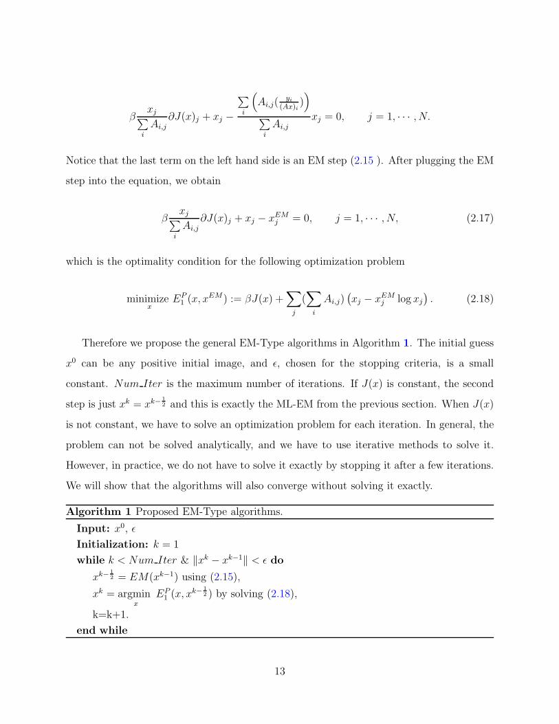
Therefore we propose the general EM-Type algorithms in Algorithm 1. The initial guess

x0 can be any positive initial image, and ǫ, chosen for the stopping criteria, is a small

constant. Num Iter is the maximum number of iterations. If J(x) is constant, the second

step is just xk = xk− 12 and this is exactly the ML-EM from the previous section. When J(x)

is not constant, we have to solve an optimization problem for each iteration. In general, the

problem can not be solved analytically, and we have to use iterative methods to solve it.

However, in practice, we do not have to solve it exactly by stopping it after a few iterations.

We will show that the algorithms will also converge without solving it exactly.

Algorithm 1 Proposed EM-Type algorithms.

Input: x0, ǫ

Initialization: k = 1

while k < Num Iter & ‖xk − xk−1‖ < ǫ do

xk− 12 = EM(xk−1) using (2.15),

xk = argminx

EP1 (x, x

k− 12 ) by solving (2.18),

k=k+1.

end while

13

2.4.1 Equivalence to EM Algorithms with a priori Information

In this subsection, the EM-Type algorithms are shown to be equivalent to EM algorithms

with a priori information. The EM algorithm is a general approach for maximizing a poste-

rior distribution when some of the data is missing [1]. It is an iterative method which alter-

nates between expectation (E) steps and maximization (M) steps. For image reconstruction,

we assume that the missing data is the latent variables zij, describing the intensity of

pixel (or voxel) j observed by detector i. Therefore the observed data are yi =∑

j

zij . We

can have the assumption that z is a realization of multi-valued random variable Z, and for

each (i, j) pair, zij follows a Poisson distribution with expected value Ai,jxj , because the

summation of two Poisson distributed random variables also follows a Poisson distribution,

whose expected value is summation of the two expected values.

The original E-step is to find the expectation of the log-likelihood given the present

variables xk:

Q(x|xk) = Ez|xk,y log p(x, z|y).

Then, the M-step is to choose xk+1 to maximize the expected log-likelihood Q(x|xk) found

in the E-step:

xk+1 = argmaxx

Ez|xk,y log p(x, z|y) = argmaxx

Ez|xk,y log(p(y, z|x)p(x))

= argmaxx

Ez|xk,y

∑

ij

(zij log(Ai,jxj)− Ai,jxj)− βJ(x)

= argminx

∑

ij

(Ai,jxj −Ez|xk,yzij log(Ai,jxj)) + βJ(x). (2.19)

From (2.19), what we need before solving it is just Ez|xk,yzij. Therefore we can compute

the expectation of missing data zij given present xk and the condition yi =∑

j

zij , denoting

this as an E-step. Because for fixed i, zij are Poisson variables with mean Ai,jxkj and

∑

j

zij = yi, the conditional distribution of zij is binomial distribution(

yi,Ai,jx

kj

(Axk)i

)

. Thus we

14

can find the expectation of zij with all these conditions by the following E-step

zk+1ij = Ez|xk,yzij =

Ai,jxkj yi

(Axk)i. (2.20)

After obtaining the expectation for all zij , we can solve the M-step (2.19).

We will show that EM-Type algorithms are exactly the described EM algorithms with a

priori information. Recalling the definition of xEM , we have

xEMj =

∑

i

zk+1ij

∑

i

Ai,j

.

Therefore, the M-step is equivalent to

xk+1 = argminx

∑

ij

(Ai,jxj − zk+1ij log(Ai,jxj)) + βJ(x)

= argminx

∑

j

(∑

i

Ai,j)(xj − xEMj log(xj)) + βJ(x).

We have shown that EM-Type algorithms are EM algorithms with a priori information. The

convergence of EM-Type algorithms is shown in the next subsection from the convergence

of the EM algorithms with a priori information.

2.4.2 Convergence of EM-Type Algorithms

In this subsection, we will show that the negative log-likelihood is decreasing in the following

theorem.

Theorem 2.4.1. The objective function (negative log-likelihood) EP (xk) in (2.16) with xk

given by Algorithm 1 will decrease until it attaints a minimum.

Proof. For all k and i, we always have the constraint satisfied

∑

j

zkij = yi.

15

Therefore, we have the following inequality

yi log(

(Axk+1)i)

− yi log(

(Axk)i)

= yi log

(

(Axk+1)i(Axk)i

)

= yi log

(

∑

j

Ai,jxk+1j

(Axk)i

)

= yi log

(

∑

j

Ai,jxkjx

k+1j

(Axk)ixkj

)

= yi log

(

∑

j

zk+1ij Ai,jx

k+1j

yiAi,jxkj

)

≥ yi∑

j

zk+1ij

yilog

(

Ai,jxk+1j

Ai,jxkj

)

(Jensen’s inequality)

=∑

j

zk+1ij log(Ai,jx

k+1j )−

∑

j

zk+1ij log(Ai,jx

kj ). (2.21)

This inequality gives us

EP (xk+1)− EP (xk) =∑

i

((Axk+1)i − yi log(Axk+1)i) + βJ(xk+1)

−∑

i

(

(Axk)i − yi log(Axk)i)

− βJ(xk)

≤∑

ij

(Ai,jxk+1j − zk+1

ij log(Ai,jxk+1j )) + βJ(xk+1)

−∑

ij

(Ai,jxkj − zk+1

ij log(Ai,jxkj ))− βJ(xk)

≤0.

The first inequality comes from (2.21) and the second inequality comes from the M-step

(2.19). When EP (xk+1) = EP (xk), these two equalities have to be satisfied. The first

equality is satisfied if and only if xk+1j = αxk

j for all j with α being a constant, while the

second one is satisfied if and only if xk and xk+1 are minimizers of the M-step (2.19). The

objective function to be minimized in M-step (2.19) is strictly convex, which means that α

has to be 1 and

βxkj∂J(x

k)j +∑

i

Ai,jxkj −

∑

i

zk+1ij = 0, j = 1, · · · , N.

16

After plugging the E-step (2.20) into these equations, we have

βxkj∂J(x

k)j +∑

i

Ai,jxkj −

∑

i

Ai,jxkj yi

(Axk)i= 0, j = 1, · · · , N.

Therefore, xk is one minimizer of the original problem.

The log-likelihood function will increase for each iteration until the solution is found, and

in the proof, we do not fully use the M-step. Even if the M-step is not solved exactly, it will

still increase as long as Q(xk+1|xk) > Q(xk|xk) is satisfied before xk converges.

The increasing of log-likelihood function can be proved in another way by using the

M-step. From xk+1 = argmaxx

Q(x|xk), we have

βxk+1j ∂J(xk+1)j +

∑

i

Ai,jxk+1j −

∑

i

zk+1ij = 0, j = 1, · · · , N.

Multiplying by (xk+1j − xk

j )/xk+1j and taking summation over j gives us

β∑

j

(xk+1j − xk

j )∂J(xk+1)j +

∑

ij

Ai,j(xk+1j − xk

j )−∑

ij

zk+1ij

xk+1j − xk

j

xk+1j

= 0.

From the convexity of J(x), we have

J(xk) ≥ J(xk+1) + (xk − xk+1)∂J(xk+1) = J(xk+1) +∑

j

(xkj − xk+1

j )∂J(xk+1)j .

Therefore we have

0 ≥ βJ(xk+1)− βJ(xk) +∑

ij

Ai,j(xk+1j − xk

j )−∑

ij

zk+1ij

xk+1j − xk

j

xk+1j

= EP (xk+1)− EP (xk) +∑

i

yi log

(

(Axk+1)i(Axk)i

)

−∑

ij

zk+1ij

xk+1j − xk

j

xk+1j

17

≥ EP (xk+1)−EP (xk) +∑

i

yi

(

1− (Axk)i(Axk+1)i

)

−∑

ij

zk+1ij

xk+1j − xk

j

xk+1j

= EP (xk+1)− EP (xk)−∑

i

yi

∑

j Ai,jxkj

∑

j Ai,jxk+1j

+∑

ij

zk+1ij

xkj

xk+1j

≥ EP (xk+1)−EP (xk).

The second inequality comes from log(x) ≥ 1 − 1/x for x > 0, and the last inequality

comes from Cauchy-Schwarz inequality. If EP (xk+1) = EP (xk), from the last inequality,

we have xk+1j = αxk

j for all j with a constant α, and from the second inequality, we have

(Axk)i = (Axk+1)i which makes α = 1. Therefore, the log-likelihood function will increase

until the solution is found.

2.4.3 EM-Type Algorithms are Alternating Minimization Methods

In this section, we will show that these algorithms can also be derived from alternating

minimization methods of other problems with variables x and z. The new optimization

problems are

minimizex,z

EP (x, z) :=∑

ij

(

zij logzij

Ai,jxj

+ Ai,jxj − zij

)

+ βJ(x).

subject to∑

j

zij = yi, i = 1, · · · ,M. (2.22)

Here EP is used again to define the new function. EP (·) means the negative log-likelihood

function of x, while EP (·, ·) means the new function of x and z defined in new optimization

problems.

Having initial guess x0, z0 of x and z, the iteration for k = 0, 1, · · · is as follows:

zk+1 = argminz

EP (xk, z), subject to∑

j

zij = yi,

xk+1 = argminx

EP (x, zk+1).

18

Firstly, in order to obtain zk+1, we fix x = xk and easily derive

zk+1ij =

Ai,jxkj yi

(Axk)i. (2.23)

After finding zk+1, let z = zk+1 fixed and update x, then we have

xk+1 = argminx

∑

ij

(

Ai,jxj + zk+1ij log

zk+1ij

Ai,jxj

)

+ βJ(x)

= argminx

∑

ij

(

Ai,jxj − zk+1ij log(Ai,jxj)

)

+ βJ(x),

which is the M-Step (2.19) in section 2.4.1. The equivalence of problems (2.16) and (2.22)

is provided in the following theorem.

Theorem 2.4.2. If (x∗, z∗) is a solution of problem (2.22), then x∗ is also a solution of

(2.16), i.e., x∗ = argminx

EP (x). If x∗ is a solution of (2.16), then we can find z∗ from

(2.23) and (x∗, z∗) is a solution of problem (2.22).

Proof. The equivalence can be proved in two steps. Firstly, we will show that EP (x, z) ≥EP (x) + C for all z, here C is a constant dependent on y only.

EP (x, z) =∑

ij

(

zij logzij

Ai,jxj+ Ai,jxj − zij

)

+ βJ(x)

=∑

ij

(

zijyi

logzij

Ai,jxj

)

yi +∑

i

((Ax)i − yi) + βJ(x)

≥∑

i

yi log

(

yi(Ax)i

)

+∑

i

((Ax)i − yi) + βJ(x)

= EP (x) +∑

i

(yi log yi − yi).

The inequality comes form Jensen’s inequality, and the equality is satisfied if and only if

zijAi,jxj

= Ci, ∀j = 1, ·, N,

where Ci are constants, which depends on x, y and i, can be found from the constraint

19

∑

j

zij = yi. Therefore minz

EP (x, z) = EP (x) + C, which means that problems (2.22) and

(2.16) are equivalent.

2.5 Simultaneous Algebraic Reconstruction Technique (SART) is

EM

Among all the iterative reconstruction algorithms, there are two important classess. One is

EM from statistical assumptions mentioned above, and the other is algebraic reconstruction

technique (ART)-type algorithms [29, 30]. Simultaneous algebraic reconstruction technique

(SART) [31, 32], as a refinement of ART, is used widely [33, 34, 35] and the convergence

analysis of SART is well studied by Jiang and Wang [36, 37], Wang and Zheng [38], Censor

and Elfving [39] and Yan [40]. In this section, we will show that SART is also an EM

algorithm, building the connection between these two classes.

From the convergence analysis of SART in [40], SART is also an algorithm for solving a

maximum likelihood problem

pY (y|x) =∏

i

1√2πwi

e−

(yi−(Ax)i)2

2wi , (2.24)

where wi =∑

j

Ai,j. Similarly, we assume that the missing data zij follow normal distribu-

tions with expected values Ai,jxj and variances Ai,j respectively. The original E-step is

to find the expectation of the log-likelihood given the present variables xk and the constraints

yi =∑

j

zij . It is easy to derive that under the constraints, zij are still realizations of nor-

mally distributed random variables, but with different expected values Ai,jxj+Ai,j(yi−(Ax)i)

wi

and variances Ai,j(wi−Ai,j)

wi respectively.

In this section, we consider the special case without regularization function, i.e., there is

no a priori information about the image to be reconstructed. The M-step is to maximize

20

the expected value of the log-likelihood function,

Ez|xk,y log p(y, z|x) = −Ez|xk,y

∑

ij

(zij −Ai,jxj)2

2Ai,j+ C (2.25)

= −∑

ij

(Ez|xk,yzij −Ai,jxj)2

2Ai,j+ C, (2.26)

where C is a constant independent of x and z. Therefore, for the E-step we have to just find

the expected value of zij given xk and the constraints, which is

zk+1ij = Ai,jx

kj +

Ai,j(yi − (Axk)i)

wi. (2.27)

For the M-step, we find xk+1 by maximizing p(y, zk+1|x) with respect to x, which has an

analytical solution

xk+1j =

∑

i

zk+1ij

∑

i

Ai,j

= xkj +

1∑

i

Ai,j

∑

i

Ai,j(yi − (Axk)i)

wi

. (2.28)

This is the original SART algorithm proposed by Andersen [31].

From the convergence analysis of SART in [40], the result of SART depends on the

initialization x0 for both noiseless and noisy cases when A is underdetermined.

Remark: SART is just one example of Landweber-like schemes for solving systems of

linear equations. By changing the variance of yi and zij , different schemes can be proposed.

For other Landweber-like schemes such as component averaging in [39, 41], they can also be

derived from the EM algorithm similarly by choosing different variances. Furthermore, new

schemes can be derived by choosing different variances.

2.6 EM-Type Algorithms for Gaussian Noise

It is shown in the last section that SART is an EM algorithm based on weighted Gaussian

assumption for the problem without regularization. Without regularization, the original

21

problem is ill-posed, and the result will depend on the initialization x0. In this section, we

will consider the regularized problem

minimizex

EG(x) := βJ(x) +∑

i

((Ax)i − yi)2

2wi, (2.29)

and derive EM-Type algorithms with Gaussian noise assumption for solving it. The E-step

is the same as in the case without regularization,

zk+1ij = Ai,jx

kj +

Ai,j(yi − (Axk)i)

wi. (2.30)

However, the M-step is different because we have a priori information on the image x to be

reconstructed. The new M-step is to solve the following optimization problems

minimizex

∑

ij

(zk+1ij − Ai,jxj)

2

2Ai,j+ βJ(x), (2.31)

which is equivalent to

minimizex

1

2

∑

j

(∑

i

Ai,j)(xj −

∑

i

zk+1ij

∑

i

Ai,j)2 + βJ(x). (2.32)

From the SART iteration (2.28) in the last section, we can define

xSART = xkj +

1∑

i

Ai,j

∑

i

Ai,j(yi − (Axk)i)

wi. (2.33)

and have

xk+1 = argminx

EG1 (x, x

SART ) :=1

2

∑

j

(∑

i

Ai,j)(xj − xSARTj )2 + βJ(x). (2.34)

Therefore, the proposed EM-Type algorithms for image reconstruction with Gaussian

noise are as follows.

22

Algorithm 2 Proposed EM-Type algorithms for Gaussian noise.

Input: x0, ǫ,

Initialization: k = 1.


xk− 12 = SART (xk−1) using (2.33)

xk = argmin EG1 (x, x

k− 12 ) by solving (2.34)

k=k+1.

end while

The initial guess x0 can be any initial image and ǫ, chosen for the stopping criteria, is

very small. Num Iter is the maximum number of iterations. When J(x) is not constant, we

have to solve an optimization problem for each iteration. In general, the problem can not be

solved analytically, and we have to use iterative methods to solve it. Similarly, we will show

that the algorithms also converge without solving the optimization problem exactly, so we

can stop it after a few iterations. The convergence analysis of these algorithms is shown in

two different ways as for the case with Poisson noise.

2.6.1 Convergence Analysis of EM-Type Algorithms for Gaussian Noise

Same as EM-Type algorithms for Poisson noise, we have convergence analysis of EM-Type

algorithms for Gaussian Noise. Firstly, we will show that the objective function (negative

log-likelihood function) is decreasing.

Theorem 2.6.1. The objective function (negative log-likelihood) EG(xk) in (2.29) with xk

given by Algorithm 2 will decrease until it attains a minimum.

Proof. Since for all k and i, we always have

∑

j

zkij = yi,

23

we have the following inequalities,

((Axk+1)i − yi)2

wi

− ((Axk)i − yi)2

wi

=

(

∑

j

Ai,j(xk+1j + xk

j )− 2yi

)(

∑

j

Ai,j(xk+1j − xk

j )

)

wi

=

(

∑

j

Ai,j

wi(xk+1

j − xkj ) +

2

wi

(

∑

j

Ai,jxkj − yi

))(

∑

j

Ai,j

wi(xk+1

j − xkj )

)

wi

≤∑

j

Ai,j

(

(xk+1j − xk

j ) +2

wi

(

∑

j

Ai,jxkj − yi

))

(xk+1j − xk

j ) (Jensen’s inequality)

=∑

j

Ai,j

(

(xk+1j − xk

j ) +2

Ai,j

(

Ai,jxkj − zk+1

ij

)

)

(xk+1j − xk

j )

=∑

j

(

(zk+1ij − Ai,jx

k+1j )2

Ai,j

−(zk+1

ij − Ai,jxkj )

2

Ai,j

)

. (2.35)

Therefore, we have

EG(xk+1)−EG(xk) =∑

i

((Axk+1)i − yi)2

2wi+ βJ(xk+1)−

∑

i

((Axk)i − yi)2

2wi− βJ(xk)

≤∑

ij

(zk+1ij − Ai,jx

k+1j )2

2Ai,j+ βJ(xk+1)−

∑

ij

(zk+1ij − Ai,jx

kj )

2

2Ai,j− βJ(xk)

≤ 0.

The first inequality comes from (2.35) and the second inequality comes from the M-step

(2.31). When EG(xk+1) = EG(xk), these two equalities have to be satisfied. The first

equality is satisfied if and only if xk+1j = xk

j + α for all j with α being a constant, while the

second one is satisfied if and only if both xk and xk+1 are minimizers of the M-step (2.31).

The objective function of this optimization problem is strictly convex, and the minimizer is

unique, which means α has to be 0. From the KKT conditions, we have

β∂J(xk)j +∑

i

Ai,jxkj −

∑

i

zk+1ij = 0 j = 1, · · · , N.

24

After plugging the E-step (2.30) into this function, we have

β∂J(x)j +∑

i

Ai,j(yi − (Axk)i)

wi= 0 j = 1, · · · , N.


We can see, from the proof above, that the optimization problem of the M-step in each

iteration does not have to be solved exactly. The log-likelihood function will still increase as

long as EG1 (x

k+1, xk+1/2) < EG1 (x

k, xk+1/2) is satisfied before xk converges.

The convergence can be proved in another way. If the M-step is solved exactly, we have

β∂J(xk+1)j +∑

i

Ai,jxk+1j −

∑

i

zk+1ij = 0.


j ) and taking summation over j gives us

β∑

j

(xk+1j − xk

j )∂J(xk+1)j +

∑

ij

Ai,jxk+1j (xk+1

j − xkj )−

∑

ij

zk+1ij (xk+1

j − xkj ) = 0.



j

(xkj − xk+1

j )∂J(xk+1)j .

Therefore we have

0 ≥ βJ(xk+1)− βJ(xk) +∑

ij

Ai,jxk+1j (xk+1

j − xkj )−

∑

ij

zk+1ij (xk+1

j − xkj )

= EG(xk+1)−EG(xk) +∑

ij

(Ai,jxk+1j − zk+1

ij )(xk+1j − xk

j )

+∑

i

(yi − (Axk)i)2 − (yi − (Axk+1)i)

2

2wi

= EG(xk+1)−EG(xk) +∑

ij

Ai,j(xk+1j − xk

j )2 −

∑

i

((Axk)i − (Axk+1)i)2

2wi

25

≥ EG(xk+1)− EG(xk) +∑

ij

Ai,j(xk+1j − xk

j )2 −

∑

i

((Axk)i − (Axk+1)i)2

wi

≥ EG(xk+1)− EG(xk).

The last inequality comes from Cauchy-Schwarz inequality and the equality holds if and only

if xk+1j = xk

j + α for all j with α being a constant. If we have EG(xk+1) = EG(xk), from the

second inequality, we have Axk = Axk+1. If constant vectors are not in the null space of A,

which is the case satisfied by all the applications mentioned above, α has to be 0.


As shown in the case of Poisson data, the algorithms can also be derived from an alternating

minimization method of other problems with variables x and z. The new problems are

minimizex,z

EG(x, z) :=∑

ij

(zij−Ai,jxj)2

2Ai,j+ βJ(x),

subject to∑

j

zij = yi, i = 1, · · ·M.(2.36)

Here EG is used again to define the new function. EG(·) means the negative log-likelihood

function of x, while EG(·, ·) means the new function of x and z defined in new optimization

problems. The iteration is as follows:

zk+1 = argminz

E(xk, z), subject to∑

j

zij = yi.

xk+1 = argminx

E(x, zk+1).

First, let us fix x = xk and update z. It is easy to derive

zk+1ij = Ai,jx

kj +

Ai,j

wi

(

yi − (Axk)i)

.

26

Then, by fixing z = zk+1 and updating x, we have

xk+1 = argminx

∑

ij

(zij − Ai,jxj)2

2Ai,j+ βJ(x)

= argminx

1

2

∑

j

(∑

i

Ai,j)(xj −

∑

i

zij

2∑

i

Ai,j)2 + βJ(x).

Since the problem (2.36) is convex, we can find the minimizer with respect to z for fixed

x first and obtain a function of x as follows,

∑

i

((Ax)i − yi)2

2wi

+ βJ(x), (2.37)

which is also convex and equals EG(x). Therefore EM-Type algorithms will converge to the

solution of (2.29).

2.6.3 Relaxation

In practice, other authors use a relaxation of SART reconstruction, which is

xk+1j = xk

j +w

∑

i

Ai,j

∑

i

Ai,j(yi − (Axk)i)

wi,

with a relaxant coefficient w. The convergence of this relaxation is shown in [36, 37, 40] for

any w ∈ (0, 2). Inspired by this strategy, we have a relaxation of the EM-Type algorithms for

image reconstruction with Gaussian noise. The EM-step is the relaxed SART with relaxant

coefficient w:

xk+ 1

2j = xk

j +w

∑

i

Ai,j

∑

i

Ai,j(yi − (Axk)i)

wi.

27

The corresponding regularization step is

xk+1 = argminx

1

2

∑

j

(∑

i

Ai,j)(xj − xk+ 1

2j )2 + wβJ(x).

When w = 1, we have already discussed the convergence in the previous subsections by EM

algorithms with a priori information and alternating minimization methods. For w 6= 1, we

will show the convergence of the relaxed EM-Type algorithms for w ∈ (0, 1) by alternating

minimization methods.

We will show that the relaxed EM-Type algorithms are equivalent to solve the uncon-

strained problems

minimizex,z

EGR (x, z) :=

∑

ij

(zij −Ai,jxj)2

2Ai,j

+ γ∑

i

(∑

j zij − yi)2

2wi

+ wβJ(x), (2.38)

where γ = w1−w

, by alternating minimization between x and z. First, fix x = xk, we can

solve the problem of z only, and the analytical solution is

zk+1ij = Ai,jx

kj +

γ

1 + γ

Ai,j

wi

(

yi − (Axk)i)

= Ai,jxkj + w

Ai,j

wi

(

yi − (Axk)i)

. (2.39)

Then let z = zk+1 fixed, and we can find xk+1 by solving

minimizex

∑

ij

(zij − Ai,jxj)2

2Ai,j+ wβJ(x) =

1

2

∑

j

(∑

i

Ai,j)(xj −

∑

i

zij∑

i

Ai,j)2 + wβJ(x) + C,

where C is a constant independent of x. Having zk+1 from (2.39), we can calculate

∑

i

zk+1ij

∑

i

Ai,j= xk

j +w

∑

i

Ai,j

∑

i

Ai,j(yi − (Axk)i)

wi= x

k+ 12

j .

Therefore this relaxed EM-Type algorithm is an alternating minimization method. We will

show next that the result of this relaxed EM-Type algorithm is the solution to (2.29).

Because the objective functional EGR (x, z) in (2.38) is convex, we can first minimize the

28

functional with respect to z with x fixed. Then the problem becomes

minimizex

γ

1 + γ

∑

i

((Ax)i − yi)2

2wi+ wβJ(x) (2.40)

= w∑

i

((Ax)i − yi)2

2wi+ wβJ(x). (2.41)

We have shown in this subsection that the relaxed EM-Type algorithm will also converge

to the solution of the original problem (2.29) when α ∈ (0, 1].

2.7 Numerical Experiments

In this section, several numerical experiments are provided to show the efficiency of EM-Type

algorithms. Though these EM-Type algorithms can be used in many applications, we choose

computed tomography (CT) image reconstruction as our application in this work. CT is a

medical imaging method which utilizes X-ray equipment to produce a two dimensional (or

three dimensional) image of the inside of an object from a large series of one dimensional (or

two dimensional) X-ray images taken along a single axis of rotation [30]. In CT reconstruc-

tion, the operator A is the Radon transform, and the discrete version of A is constructed by

Siddon’s algorithm [42, 43].

We recall the continuous Radon transform in two dimensions, applied to an image func-

tion f(x, y): assuming that a straight line in the plane can be represented by the equation

depending on two parameters (θ, t),

x cos θ + y sin θ = t,

the Radon transform f 7→ g (with (θ, t) 7→ g(θ, t) the image in the sinogram domain (θ, t)

of the function (x, y) 7→ f(x, y)) is defined by the projections along lines of f ,

g(θ, t) =

∫ +∞

−∞

∫ +∞

−∞

f(x, y)δ(x cos θ + y sin θ − t)dxdy,

29

where δ is the one-dimensional Dirac delta function, with support on the line of equation

x cos θ + y sin θ = t. In the two-dimensional discrete case, f represents a discrete image

matrix and g (or a noisy version of g) is known only at a finite number of samples (θi, ti).

In computed tomography, we must recover f from its projections g. Although the Radon

transform is an invertible operator, in the real discrete case only a small finite number of

projections (θi, ti) are given, which may be also noisy. Thus, in the real case, the recovery

of f from projections g is a difficult inverse problem. For the rest of the presentation, we

will continue to use the notations x for the image to be recovered, y for the measurements

or projections in the sinogram domain, and A for the discrete Radon transform with a finite

number of samples.

The problem is to reconstruct the image from the measurements, which is equivalent to

solving Ax = y. Poisson noise is assumed. Total variation (TV) and a modified version of

TV are chosen to be the regularization. In order to compare the results of different methods,

root mean square error (RMSE) is utilized.

2.7.1 CT Reconstruction by EM-TV (2D)

At first, we illustrate one method (EM-TV) at a simple synthetic object (two dimensional

256x256 Shepp-Logan phantom), see Figure 2.1.

Original x

Figure 2.1: 2D Shepp-Logan phantom

The most common method used in commercial CT is filtered back projection (FBP),

which is straightforward to implement and can be computed rapidly. However, FBP has

limitations due to the presence of streak artifacts and noise enhancement, which is inherent

30

in the reconstruction. Furthermore, in order to obtain an accurate image, many views are

taken. Algorithms that can perform accurate image reconstruction from few views are very

important in reducing patient dose and speeding up scans. Optimization based methods,

including EM-TV, can reconstruct images from few views, but require more computing time.

However, with the development of graphics processing units (GPUs), the computing time

has been reduced greatly and this kind of technique becomes more and more important.

In the following experiment, we will compare the reconstruction results obtained by

EM-TV with those obtained by filtered back projection. To solve the above minimization

problem (2.18) with J(x) being the total variation, we use an iterative semi-implicit finite-

differences scheme. Each iteration is called a TV step. Given xEM , already computed from

the EM step, we compute the new x discretizing (2.17) (as a discrete minimizer of (2.18)),

by the following simple iterative scheme, presented below in two spatial dimensions and

assuming now that x is represented as a 2D matrix: from an initial guess x0, we compute

xn+1 with n ≥ 0 from the following linearized discrete equation,

− βxni,j

vi,j

xni+1,j − xn+1

i,j√

ǫ+ (xni+1,j − xn

i,j)2 + (xn

i,j+1 − xni,j)

2

+ βxni,j

vi,j

xn+1i,j − xn

i−1,j√

ǫ+ (xni,j − xn

i−1,j)2 + (xn

i−1,j+1 − xni−1,j)

2

− βxni,j

vi,j

xni,j+1 − xn+1

i,j√

ǫ+ (xni+1,j − xn

i,j)2 + (xn

i,j+1 − xni,j)

2

+ βxni,j

vi,j

xn+1i,j − xn

i,j−1√

ǫ+ (xni+1,j−1 − xn

i,j−1)2 + (xn

i,j − xni,j−1)

2+ xn+1

i,j − xEMi,j = 0, (2.42)

where ǫ is a small constant and vi,j =∑M

i′=1Ai′,j′ with j′ being the index corresponding to

the 2D index (i, j).

Finally, the two steps (EM and TV) are solved in an alternating fashion. Usually, for

each main iteration, we apply 2 or 3 EM steps, followed by 5 to 8 TV steps. For the TV

step, the initial guess can be defined as the result from the previous EM update, or from the

last TV update [16].

31

The measurements are obtained using Siddon’s algorithm. We consider both the noise-

free and noisy cases. For the FBP method, we present results using 36 views (every 10

degrees; for each view there are 301 measurements), 180 views, and 360 views. In order to

show that we can reduce the number of views by using EM-TV, we only use 36 views for

the proposed method. The results are shown in Figure 2.2. We notice the much improved

results obtained with EM-TV using only 36 views, by comparison with FBP using 36, 180

or even 360 views.

Noise-free caseFBP 36 views FBP 180 views FBP 360 views EM-TV 36 views

RMSE = 50.8394 RMSE = 14.1995 RMSE = 12.6068 RMSE = 2.3789

Noisy caseFBP 36 views FBP 180 views FBP 360 views EM-TV 36 views

RMSE = 51.1003 RMSE = 14.3698 RMSE = 12.7039 RMSE = 3.0868

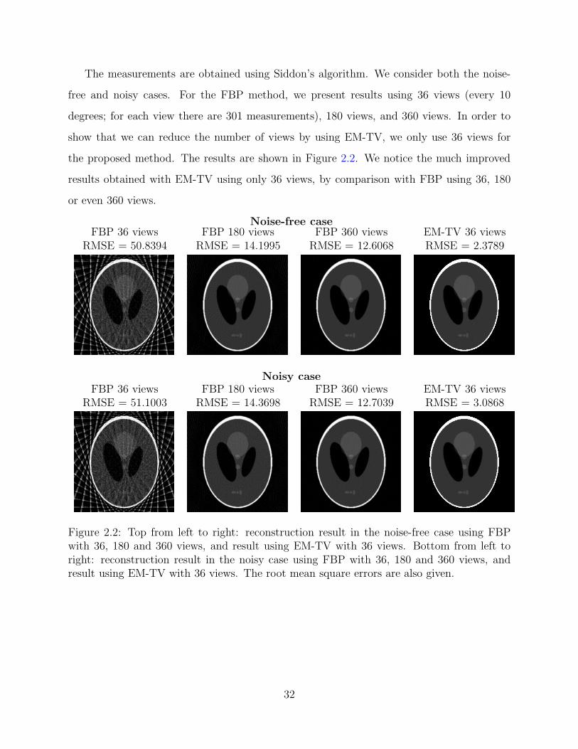
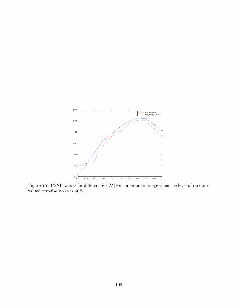
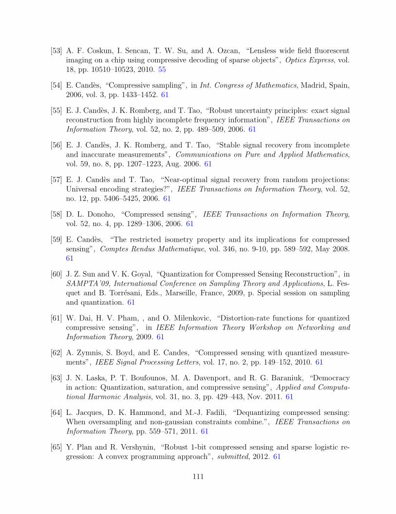
Figure 2.2: Top from left to right: reconstruction result in the noise-free case using FBPwith 36, 180 and 360 views, and result using EM-TV with 36 views. Bottom from left toright: reconstruction result in the noisy case using FBP with 36, 180 and 360 views, andresult using EM-TV with 36 views. The root mean square errors are also given.

32

2.7.2 Reconstruction using EM-MSTV (2D)

Instead of TV regularization, we also show the results by using a modified TV, which is

called Mumford-Shah TV (MSTV) [44]. The new regularization is

J(x, v) =

∫

Ω

v2|∇x|+ α

∫

Ω

(

ǫ|∇v|2 + (v − 1)2

4ǫ

)

,

which has two variables x and v, and Ω is the image domain. It is shown by Alicandro et

al. [45] that J(x, v) will Γ-convergent to

∫

Ω\K

|∇x|+ α

∫

K

|x+ − x−|1 + |x+ − x−|dH

1 + |Dcx|(Ω),

where x+ and x− denote the image values on two sides of the edge set K, H1 is the one-

dimensional Hausdorff measure and Dcx is the Cantor part of the measure-valued derivative

Dx.

The comparisons of EM-TV and EM-MSTV in both noise-free and noisy cases are in

Figure 2.3. From the results, we can see that with MSTV, the reconstructed images will be

better than with TV only, visually and according to the RMSE.

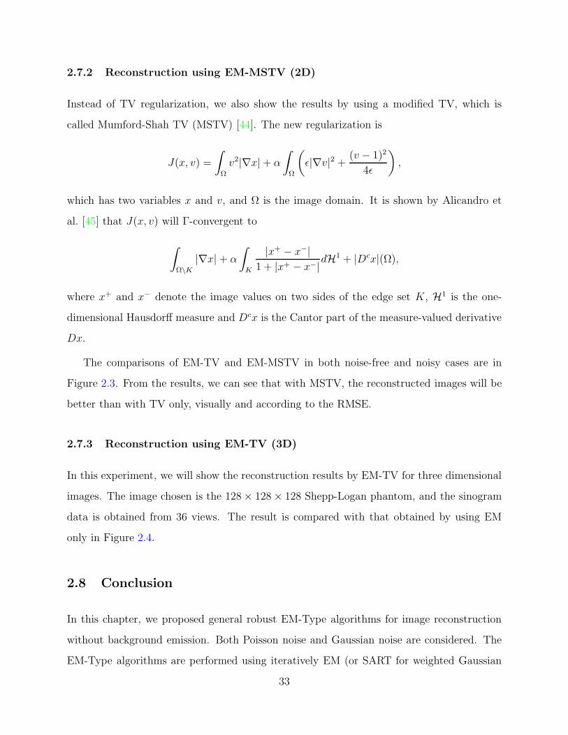
2.7.3 Reconstruction using EM-TV (3D)

In this experiment, we will show the reconstruction results by EM-TV for three dimensional

images. The image chosen is the 128× 128× 128 Shepp-Logan phantom, and the sinogram

data is obtained from 36 views. The result is compared with that obtained by using EM

only in Figure 2.4.

2.8 Conclusion

In this chapter, we proposed general robust EM-Type algorithms for image reconstruction

without background emission. Both Poisson noise and Gaussian noise are considered. The

EM-Type algorithms are performed using iteratively EM (or SART for weighted Gaussian

33

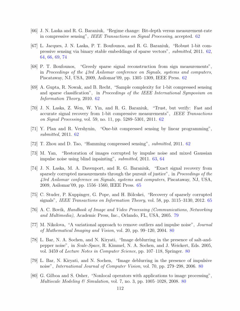
TV without noise MSTV without noise TV with noise MSTV with noiseRMSE = 2.33 RMSE = 1.58 RMSE = 3.33 RMSE = 2.27

−0.15

−0.1

−0.05

0

0.05

0.1

0.15

−0.1

−0.08

−0.06

−0.04

−0.02

0

0.02

0.04

0.06

0.08

0.1

−0.25

−0.2

−0.15

−0.1

−0.05

0

0.05

0.1

0.15

0.2

−0.15

−0.1

−0.05

0

0.05

0.1

0.15

Figure 2.3: Comparisons of TV regularization and MSTV regularization for both withoutand with noise cases. Top row shows the reconstructed images by these two methods inboth cases, Bottom row shows the differences between the reconstructed images and originalphantom image. The RMSEs and differences show that MSTV can provide better resultsthan TV only.

noise) and regularization in the image domain. The convergence of these algorithms is proved

in several ways: EM with a priori information and alternating minimization methods. To

show the efficiency of EM-Type algorithms, the application in CT reconstruction is chosen.

We compared EM-TV and EM-MSTV for 2D CT reconstruction. Both methods can give us

good results by using undersampled data comparing to the filtered back projection. Results

from EM-MSTV have sharper edges than those from EM-TV. Also EM-TV is used for 3D

CT reconstruction and the performance is better than using EM only (without regularization

term) for undersampled data.

34

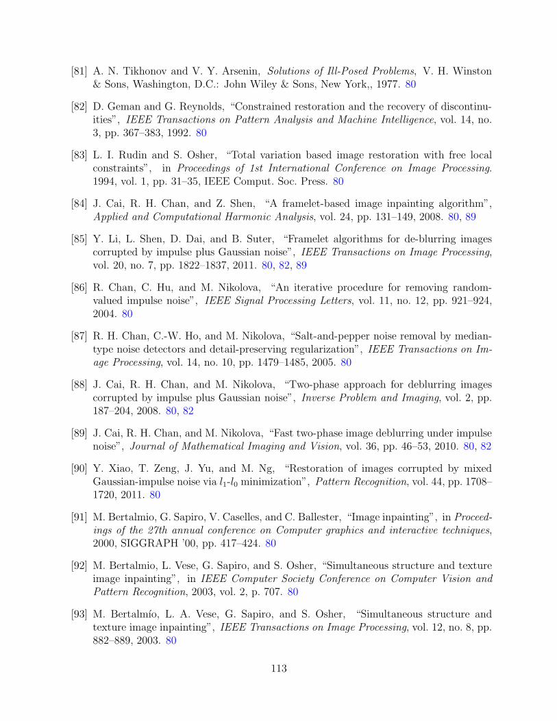
original EM-TV (RMSE=3.7759) EM (RMSE=31.9020)

z-direction

x-direction

y-direction

Figure 2.4: Reconstruction results in three dimensions for the noise-free case. First column:two-dimensional views of the original three-dimensional Shepp-Logan phantom. Middle col-umn: two-dimensional views of reconstruction results obtained using EM-TV algorithm.Last column: two-dimensional views of reconstruction results obtained using EM iteration.The root mean square errors are also given.

35

CHAPTER 3

General Convergent EM-Type Algorithms for Image

Reconstruction With Background Emission and

Poisson Noise

3.1 Introduction

As mentioned in the previous chapter, the degradation model can be formulated as a linear

inverse and ill-posed problem,

y = Ax+ b+ n. (3.1)

Here, y is the measured data (vector in RM for the discrete case). A is a compact operator

(matrix in RM×N for the discrete case). For all the applications we will consider, the entries

of A are nonnegative and A does not have full column rank. x is the desired exact image

(vector in RN for the discrete case). b is the background emission, which is assumed to be

known, and n is the noise. In the last chapter, we considered the case without background

emission (b = 0), and the case with background emission (b 6= 0) is considered in this chapter.

In astronomy, this is due to sky emission [46, 47], while in fluorescence microscopy, it is due

to auto-fluorescence and reflections of the excitation light. Since the matrix A does not have

full column rank, the computation of x directly by finding the inverse of A is not reasonable

because (3.1) is ill-posed and n is unknown. Therefore regularization techniques are needed

for solving these problems efficiently.

Same as in the last chapter, we assume that measured data y is a realization of a multi-

valued random variable, denoted by Y and the image x is also considered as a realization of

another multi-valued random variable, denoted by X . Therefore the Bayesian formula gives

36

us

pX(x|y) =pY (y|x)pX(x)

pY (y). (3.2)

This is a conditional probability of having X = x given that y is the measured data. After

inserting the detected value of y, we obtain a posteriori probability distribution of X . Then

we can find x∗ such that pX(x|y) is maximized, as maximum a posteriori (MAP) likelihood

estimation.

In general, X is assigned as a Gibbs random field, which is a random variable with the

following probability distribution

pX(x) ∼ e−βJ(x), (3.3)

where J(x) is a given convex energy functional, and β is a positive parameter. The choice

of pY (y|x) depends on the noise model. If the random variable Y of the detected values y

follows a Poisson distribution [20, 21] with an expectation value provided by Ax+ b, we have

yi ∼ Poisson(Ax+ b)i, i.e., pY (y|x) ∼∏

i

(Ax+ b)yiiyi!

e−(Ax+b)i . (3.4)

By minimizing the negative log-likelihood function, we obtain the following optimization

problem

minimizex≥0

∑

i

(

(Ax+ b)i − yi log(Ax+ b)i)

+ βJ(x). (3.5)

In this chapter, we will focus on solving (3.5). It is easy to see that the objective function

in (3.5) is convex when J(x) is convex. Additionally, with suitably chosen regularization

J(x), the objective function is strictly convex, and the solution to this problem is unique.

The work is organized as follows. In section 3.2, we will give a short introduction of

expectation maximization (EM) iteration, or the Richardson-Lucy algorithm, used in image

reconstruction with background emission from the view of optimization. In section 3.3, we

will propose general EM-Type algorithms for image reconstruction with background emission

when the measured data is corrupted by Poisson noise. This is based on the maximum a

37

posteriori likelihood estimation and EM step. In this section, these EM-Type algorithms are

shown to be equivalent to EM algorithms with a priori information, and their convergence

is shown in two different ways. In addition, these EM-Type algorithms are also considered

as alternating minimization methods for equivalent optimization problems. For the case

without regularization, more analysis on the convergence (the distance to the solution is

decreasing) is provided. However, for some regularizations, the reconstructed images will

lose contrast. To overcome this problem, EM-Type algorithms with Bregman iteration are

introduced in section 3.4. Some numerical experiments are given in section 3.5 to show the

efficiency of the EM-Type algorithms with different regularizations. We will end this work

by a short conclusion section.

3.2 Expectation Maximization (EM) Iteration

A maximum likelihood (ML) method for image reconstruction based on Poisson data was

introduced by Shepp and Vardi [21] in 1982 for applications in emission tomography. In fact,

this algorithm was originally proposed by Richardson [23] in 1972 and Lucy [24] in 1974 for

astronomy. In this section, we consider the special case without regularization term, i.e.,

J(x) is a constant, we do not have any a priori information about the image. From equation

(3.4), for given measured data y, we have a function of x, the likelihood of x, defined by

pY (y|x). Then a ML estimate of the unknown image is defined as any maximizer x∗ of

pY (y|x).

By taking the negative log-likelihood, one obtains, up to an additive constant

f0(x) =∑

i

(

(Ax+ b)i − yi log(Ax+ b)i)

, (3.6)

and the problem is to minimize this function f0(x) on the nonnegative orthant, because we

have the constraint that the image x is nonnegative. In fact, we have

f(x) = DKL(y, Ax+ b) :=∑

i

(

yi logyi

(Ax+ b)i+ (Ax+ b)i − yi

)

= f0(x) + C,

38

where DKL(y, Ax+ b) is the Kullback-Leibler (KL) divergence of Ax+ b from y, and C is a

constant independent of x. The KL divergence is considered as a data-fidelity function for

Poisson data just like the standard least-square ‖Ax+b−y‖22 is the data-fidelity function for

additive Gaussian noise. It is convex, nonnegative and coercive on the nonnegative orthant,

so the minimizers exist and are global.

In order to find a minimizer of f(x) with the constraint x ≥ 0, we can solve the Karush-

Kuhn-Tucker (KKT) conditions [25, 26],

∑

i

(

Ai,j(1−yi

(Ax+ b)i)

)

− sj = 0, j = 1, · · · , N,

sj ≥ 0, xj ≥ 0, j = 1, · · · , N,

sTx = 0.



j = 1, · · · , N . Multiplying by xj gives us

∑

i

(

Ai,j(1−yi

(Ax+ b)i)

)

xj = 0, j = 1, · · · , N. (3.7)

Therefore, we have the following iterative scheme

xk+1j =

∑

i

(

Ai,j(yi

(Axk+b)i))

∑

i

Ai,j

xkj . (3.8)

This is the well-known EM iteration or Richardson-Lucy algorithm in image reconstruction,

and an important property of it is that it preserves positivity. If xk is positive, then xk+1 is

also positive if A preserves positivity.

Shepp and Vardi showed in [21] that when b = 0, this is equivalent to the EM algorithm

proposed by Dempster, Laird and Rubin [1]. Actually, when b 6= 0, this is also equivalent to

the EM algorithm and it will be shown in the next section. To make it clear, EM iteration

means the special EM method used in image reconstruction, while EM algorithm means the

39

general EM algorithm for solving missing data problems.

3.3 EM-Type Algorithms for Image Reconstruction

The method shown in the last section is also called maximum-likelihood expectation maxi-

mization (ML-EM) reconstruction, because it is a maximum likelihood approach without any

Bayesian assumption on the images. If additional a priori information about the image is

given, we have maximum a posteriori probability (MAP) approach [27, 28], which is the case

with regularization term J(x). Again we assume here that the detected data is corrupted

by Poisson noise, and the regularization problem is

minimizex

EP (x) := βJ(x) +∑

i

((Ax+ b)i − yi log(Ax+ b)i) ,

subject to xj ≥ 0, j = 1, · · · , N.

(3.9)

This is still a convex constraint optimization problem when J(x) is convex and we can find

the optimal solution by solving the KKT conditions:

β∂J(x)j +∑

i

(

Ai,j(1−yi

(Ax+ b)i)

)

− sj = 0, j = 1, · · · , N,

sj ≥ 0, xj ≥ 0, j = 1, · · · , N,

sTx = 0.



j = 1, · · · , N . Thus we obtain

βxj∂J(x)j +∑

i

(

Ai,j(1−yi

(Ax+ b)i)

)

xj = 0, j = 1, · · · , N,

40

or equivalently

βxj

∑

i

Ai,j

∂J(x)j + xj −

∑

i

(

Ai,j(yi

(Ax+b)i))

∑

i

Ai,j

xj = 0, j = 1, · · · , N.

Notice that the last term on the left hand side is an EM step (3.8). After plugging the EM

step into the equation, we obtain

βxj

∑

i

Ai,j

∂J(x)j + xj − xEMj = 0, j = 1, · · · , N,

which is the optimality condition for the following optimization problem

minimizex

EP1 (x, x

EM) := βJ(x) +∑

j

(∑

i

Ai,j)(

xj − xEMj log xj

)

. (3.10)

Therefore we propose the general EM-Type algorithms in Algorithm 3. The initial guess

x0 can be any positive initial image, and ǫ, chosen for the stopping criteria, is very small.

Num Iter is the maximum number of iterations. If J(x) is constant, the second step is

just xk = xk− 12 and this is exactly the ML-EM from the previous section. When J(x) is

not constant, we have to solve an optimization problem for each iteration. In general, the

problem can not be solved analytically, and we have to use iterative methods to solve it.

However, in practice, we do not have to solve it exactly by stopping it after a few iterations.

We will show that the algorithms will also converge without solving it exactly.

Algorithm 3 Proposed EM-Type algorithms.

Input: x0, ǫ

Initialization: k = 1


xk− 12 = EM(xk−1) using (3.8)

xk = argmin EP1 (x, x

k− 12 ) by solving (3.10)

k=k+1

end while

41

3.3.1 Equivalence to EM Algorithms with a priori Information

In this subsection, the EM-Type algorithms are shown to be equivalent to EM algorithms

with a priori information. The EM algorithm is a general approach for maximizing a pos-

terior distribution when some of the data is missing [1]. It is an iterative method that

alternates between expectation (E) steps and maximization (M) steps. For image recon-

struction, we assume that the missing data is zij, describing the intensity of pixel (or

voxel) j observed by detector i and bi, the intensity of background observed by detector

i. Therefore the observed data are yi =∑

j

zij + bi. We can have the assumption that z is a

realization of multi-valued random variable Z, and for each (i, j) pair, zij follows a Poisson

distribution with expected value Ai,jxj , and bi follows a Poisson distribution with expected

value bi, because the summation of two Poisson distributed random variables also follows a

Poisson distribution, whose expected value is summation of the two expected values.

The original E-step is to find the expectation of the log-likelihood given the present

variables xk:

Q(x|xk) = Ez|xk,y log p(x, z|y)

Then, the M-step is to choose xk+1 to maximize the expected log-likelihood Q(x|xk) found

in the E-step:

xk+1 = argmaxx

Ez|xk,y log p(x, z|y) = argmaxx

Ez|xk,y log(p(y, z|x)p(x))

= argmaxx

Ez|xk,y

∑

ij

(zij log(Ai,jxj)−Ai,jxj)− βJ(x)

= argminx

∑

ij

(Ai,jxj − Ez|xk,yzij log(Ai,jxj)) + βJ(x). (3.11)

From (3.11), what we need before solving it is just Ez|xk,yzij. Therefore we compute the

expectation of missing data zij given present xk, denoting this as an E-step. Because for

fixed i, zij are Poisson variables with mean Ai,jxkj and bi is Poisson variable with mean

bi, then the distribution of zij is binomial distribution(

yi,Ai,jxk

j

(Axk+b)i

)

, thus we can find the

42

expectation of zij with all these conditions by the following E-step

zk+1ij = Ez|xk,yzij =

Ai,jxkj yi

(Axk + b)i, bk+1

i =biyi

(Axk + b)i. (3.12)

After obtaining the expectation for all zij , then we can solve the M-step (3.11).

We will show that EM-Type algorithms are exactly the described EM algorithms with a

priori information. Recalling the definition of xEM , we have

xEMj =

∑

i

zk+1ij

∑

i

Ai,j

. (3.13)

Therefore, the M-step is equivalent to

xk+1 = argminx

∑

ij

(Ai,jxj − zk+1ij log(Ai,jxj)) + βJ(x)

= argminx

∑

j

(∑

i

Ai,j)(xj − xEMj log(xj)) + βJ(x).

We have shown that EM-Type algorithms are EM algorithms with a priori information. The

convergence of EM-Type algorithms is shown in the next subsection from the convergence

of the EM algorithms with a priori information.

3.3.2 Convergence of EM-Type Algorithms

In this subsection, we will show that the negative log-likelihood is decreasing in the following

theorem.

Theorem 3.3.1. The objective function (negative log-likelihood) EP (xk) in (3.9) with xk

given by Algorithm 3 will decrease until it attaints a minimum.

Proof. For all k and i, we always have the constraint satisfied

∑

j

zkij + bki = yi.

43

Therefore, we have the following inequality

yi log(

(Axk+1 + b)i)

− yi log(

(Axk + b)i)

= yi log

(

(Axk+1 + b)i(Axk + b)i

)

= yi log

∑

j

Ai,jxk+1j + bi

(Axk + b)i

= yi log

(

∑

j

Ai,jxkjx

k+1j

(Axk + b)ixkj

+bi

(Axk + b)i

)

= yi log

(

∑

j

zk+1ij Ai,jx

k+1j

yiAi,jxkj

+bk+1i

yi

)

≥ yi∑

j

zk+1ij

yilog

(

Ai,jxk+1j

Ai,jxkj

)

(Jensen’s inequality)

=∑

j

zk+1ij log(Ai,jx

k+1j )−

∑

j

zk+1ij log(Ai,jx

kj ). (3.14)

This inequality gives us

EP (xk+1)−EP (xk) =∑

i

((Axk+1 + b)i − yi log(Axk+1 + b)i) + βJ(xk+1)

−∑

i

(

(Axk + b)i − yi log(Axk + b)i

)

− βJ(xk)

≤∑

ij

(Ai,jxk+1j − zk+1

ij log(Ai,jxk+1j )) + βJ(xk+1)

−∑

ij

(Ai,jxkj − zk+1

ij log(Ai,jxkj ))− βJ(xk)

≤ 0.

The first inequality comes from (3.14) and the second inequality comes from the M-

step (3.11). When EP (xk+1) = EP (xk), these two equalities have to be satisfied. The first

equality is satisfied if and only if xk+1j = xk

j for all j, while the second one is satisfied if and

only if xk and xk+1 are minimizers of the M-step (3.11). Since the objective function to be

44

minimized in M-step (3.11) is strictly convex, we have

βxkj∂J(x

k)j +∑

i

Ai,jxkj −

∑

i

zk+1ij = 0, j = 1, · · · , N,

after plugging the E-step (3.12) into these equations, we have

βxkj∂J(x

k)j +∑

i

Ai,jxkj −

∑

i

Ai,jxkj yi

(Axk + b)i= 0, j = 1, · · · , N.


The log-likelihood function will increase for each iteration until the solution is found, and

from the proof, we do not fully use the M-step. Even if the M-step is not solved exactly, it

will still increase as long as Q(xk+1|xk) > Q(xk|xk) is satisfied before xk converges.

The increasing of log-likelihood function can be proved in another way by using the

M-step. From xk+1 = argmaxx

Q(x|xk), we have

βxk+1j ∂J(xk+1)j +

∑

i

Ai,jxk+1j −

∑

i

zk+1ij = 0, j = 1, · · · , N.


j )/xk+1j and taking summation over j gives us

β∑

j

(xk+1j − xk

j )∂J(xk+1)j +

∑

ij

Ai,j(xk+1j − xk

j )−∑

ij

zk+1ij

xk+1j − xk

j

xk+1j

= 0.



j

(xkj − xk+1

j )∂J(xk+1).

Therefore we have

0 ≥ βJ(xk+1)− βJ(xk) +∑

ij

Ai,j(xk+1j − xk

j )−∑

ij

zk+1ij

xk+1j − xk

j

xk+1j

45

= EP (xk+1)− EP (xk) +∑

i

yi log

(

(Axk+1 + b)i(Axk + b)i

)

−∑

ij

zk+1ij

xk+1j − xk

j

xk+1j

≥ EP (xk+1)−EP (xk) +∑

i

yi

(

1− (Axk + b)i(Axk+1 + b)i

)

−∑

ij

zk+1ij

xk+1j − xk

j

xk+1j

= EP (xk+1)− EP (xk)−∑

i

yi

∑

j Ai,jxkj + bi

∑

j Ai,jxk+1j + bi

+∑

ij

zk+1ij

xkj

xk+1j

+∑

i

(yi −∑

j

zk+1ij )

≥ EP (xk+1)−EP (xk).

The second inequality comes from log(x) ≥ 1− 1/x for x > 0, and the last inequality comes

from Cauchy-Schwarz inequality. If EP (xk+1) = EP (xk), from the last inequality, we have

xk+1j = xk

j for all j. Therefore, the log-likelihood function will increase until the solution is

found.


In this section, we will show that these algorithms can also be derived from alternating

minimization methods of other problems with variables x and z. The new optimization

problems are

minimizex,z

EP (x, z) :=∑

ij

(

zij logzij

Ai,jxj

+ Ai,jxj − zij

)

+∑

i

(

bi logbibi

+ bi − bi

)

+ βJ(x), (3.15)

where bi = yi−∑

j

zij , for all i = 1, · · · ,M. Here EP is used again to define the new function.

EP (·) means the negative log-likelihood function of x, while EP (·, ·) means the new function

of x and z defined in new optimization problems.

Having initial guess x0, z0 of x and z, the iteration for k = 0, 1, · · · is as follows:

zk+1 = argminz

EP (xk, z),

xk+1 = argminx

EP (x, zk+1).

46

Firstly, in order to obtain zk+1, we fix x = xk and easily derive

zk+1ij =

Ai,jxkj yi

(Axk + b)i. (3.16)

After finding zk+1, let z = zk+1 fixed and update x, then we have

xk+1 = argminx

∑

ij

(

Ai,jxj + zk+1ij log

zk+1ij

Ai,jxj

)

+ βJ(x)

= argminx

∑

ij

(

Ai,jxj − zk+1ij log(Ai,jxj)

)

+ βJ(x),

which is the M-Step (3.11) in section 3.3.1. The equivalence of problems (3.9) and (3.15) is

provided in the following theorem.

Theorem 3.3.2. If (x∗, z∗) is a solution of problem (3.15), then x∗ is also a solution of

(3.9), i.e., x∗ = argminx

EP (x). If x∗ is a solution of (3.9), then we can find z∗ from (3.16)

and (x∗, z∗) is a solution of problem (3.15).

Proof. The equivalence can be proved in two steps. Firstly, we will show that EP (x, z) ≥EP (x) + C for all z, here C is constant dependent on y only:

EP (x, z) =∑

ij

(

zij logzij

Ai,jxj+ Ai,jxj − zij

)

+∑

i

(

bi logbibi

+ bi − bi

)

+ βJ(x)

=∑

ij

(

zijyi

logzij

Ai,jxj

)

yi +∑

i

biyi

logbibiyi +

∑

i

((Ax+ b)i − yi) + βJ(x)

≥∑

i

yi log

(

yi(Ax+ b)i

)

+∑

i

(

(Ax+ b)i − yi)

+ βJ(x)

= EP (x) +∑

i

(yi log yi − yi).

The inequality comes form Jensen’s inequality, and the equality is satisfied if and only if

zijAi,jxj

=bibi

= Ci, ∀j = 1, · · · , N, (3.17)

where Ci are constants, which depends on x, y and i and can be found from the constraint

47

∑

j zij + bi = yi. Therefore minz

EP (x, z) = EP (x) + C, which means that problems (3.15)

and (3.9) are equivalent.

From these two convergence analyses, if the second part of the EM-Type algorithms can

not be solved exactly, we can choose the initial guess to be the result from the previous

iteration, then use any method for solving convex optimization problem to obtain a better

result.

3.3.4 Further Analysis for the Case Without Regularization

For the case without regularization, we will show that for each limit point x of the sequence

xk, we have DKL(x, xk+1) ≤ DKL(x, x

k) if∑

i

Ai,j = 1 for all j. If this condition is not

fulfilled, similarly, we can show that DKL(x′, xk+1′) ≤ DKL(x

′, xk ′), where x′j =

∑

i

Ai,jxj and

xk ′j =

∑

i

Ai,jxkj for all j.

Theorem 3.3.3. If∑

i

Ai,j = 1 for all j, DKL(x, xk) is decreasing for the case without

regularization.

Proof. Define vectors f j, gj such that their components are

f ji =

Ai,jyi/(Ax+ b)i(AT (y/(Ax+ b)))j

, gji =Ai,jyi/(Ax

k + b)i(AT (y/(Axk + b)))j

, i = 1, · · ·n, (3.18)

then we have∑

i

f ji =

∑

i

gji = 1 and

0 ≤∑

j

xjDKL(fj, gj)

=∑

j

xj

∑

i

f ji log

f ji

gji

=∑

j

xj

∑

i


log(Axk + b)i(A

T (y/(Axk + b)))j(Ax+ b)i(AT (y/(Ax+ b)))j

=∑

j

xj

∑

i


log(Axk + b)ix

k+1j xj

(Ax+ b)ixjxkj

.

48

Since

xj =(AT (y/(Ax+ b))j)

(AT1)jxj ,

we have

(AT (y/(Ax+ b)))j(AT1)j

= 1.

It follows that

0 ≤∑

j

xj

∑

i

Ai,jyi(Ax+ b)i

log(Axk + b)ix

k+1j

(Ax+ b)ixkj

=∑

j

xj

∑

i

Ai,jyi(Ax+ b)i

(

log(Axk + b)i(Ax+ b)i

+ logxk+1j

xkj

)

=∑

j

xj

∑

i

Ai,jyi(Ax+ b)i


+∑

j

xj logxk+1j

xkj

=∑

i

(Ax)iyi(Ax+ b)i


+∑

j

xj logxk+1j

xkj

= DKL(y, Ax+ b)−DKL(y, Axk + b) +DKL(x, x

k)−DKL(x, xk+1)

−∑

i

biyi(Ax+ b)i


−∑

j

xj +∑

j

xk+1j .

Since∑

i

yi −∑

j

xk+1j =

∑

i

(yi −∑

j

zk+1ij ) =

∑

i

biyi(Axk+b)i

, we have

−∑

i

biyi(Ax+ b)i


−∑

j

xj +∑

j

xk+1j

=−∑

i

biyi(Ax+ b)i


+∑

i

biyi(Ax+ b)i

−∑

i

biyi(Axk + b)i

=−DKL(biyi

(Ax+ b)i,

biyi(Axk + b)i

) ≤ 0.

The decreasing of the objective functionDKL(y, Axk+b) gives usDKL(y, Ax+b) ≤ DKL(y, Ax

k+

49

b) and it follows that

0 ≤ DKL(x, xk)−DKL(x, x

k+1)

which is DKL(x, xk+1) ≤ DKL(x, x

k).

If∑

i

Ai,j = 1 is not satisfied, we have the same property for x′ and xk ′, which are just

weighted vectors with the jth weight being∑

i

Ai,j, from the same proof.

3.4 EM-Type Algorithms with Bregman Iteration

In the previous section, the EM-Type algorithms are presented to solve problem (3.9). How-

ever, the regularization may lead to reconstructed images suffering from contrast reduc-

tion [48]. Therefore, we suggest a contrast improvement in EM-Type algorithms by Breg-

man iteration, which is introduced in [49, 50, 51]. An iterative refinement is obtained from

a sequence of modified EM-Type algorithms.

For the problem with Poisson noise, we start with the basic EM-Type algorithms, i.e.,

finding the minimum x1 of (3.9). After that, variational problems with a modified regular-

ization term

xk+1 = argminx

β(J(x)− 〈pk, x〉) +∑

i

((Ax+ b)i − yi log(Ax+ b)i) (3.19)

where pk ∈ ∂J(xk), are solved sequentially. From the optimality of (3.19), we have the

following formula for updating pk+1 from pk and xk+1:

pk+1 = pk − 1

βAT

(

1− y

Axk+1 + b

)

. (3.20)

Therefore the EM-Type algorithms with Bregman iteration are as follows:

50

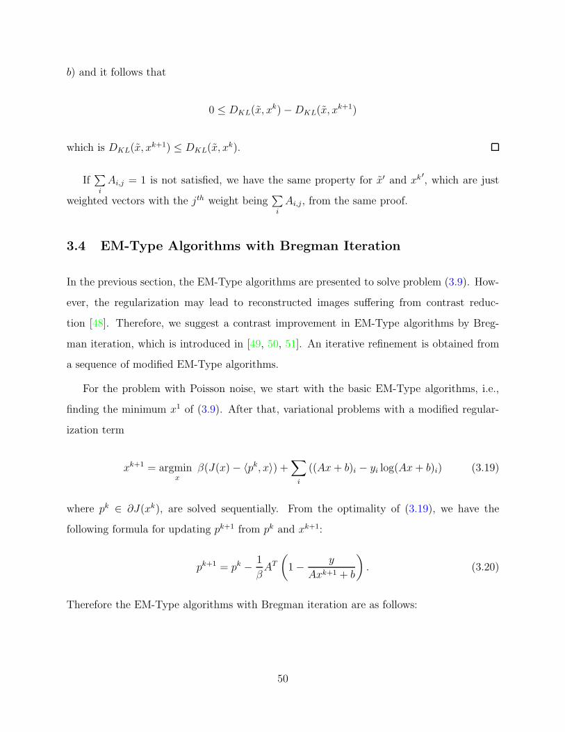
Algorithm 4 Proposed EM-Type algorithms with Bregman iteration.

Input: x0, δ, ǫ

Initialization: k = 1, p0 = 0

while k ≤ Num outer & DKL(y, Axk−1 + b) < δ do

xtemp,0 = xk−1, l = 0,

while l ≤ Num inner & ‖xtemp,l − xtemp,l−1‖ ≤ ǫ do

l = l + 1,

xtemp,l− 12 = EM(xtemp,l−1) using (3.8),

xtemp,l = argminx

EP1 (x, x

temp,l− 12 ) with J(x)− 〈pk−1, x〉

end while

xk = xtemp,l

pk = pk−1 − 1βAT

(

1− yAxk + b

)

,

k=k+1

end while

The initial guess x0 can be any positive image, and δ = DKL(y, Ax∗+ b), where x∗ is the

ground truth, is assumed to be known, ǫ is the stopping criteria which is small. Num inner

and Num outer are maximum numbers of inner iterations and outer iterations.

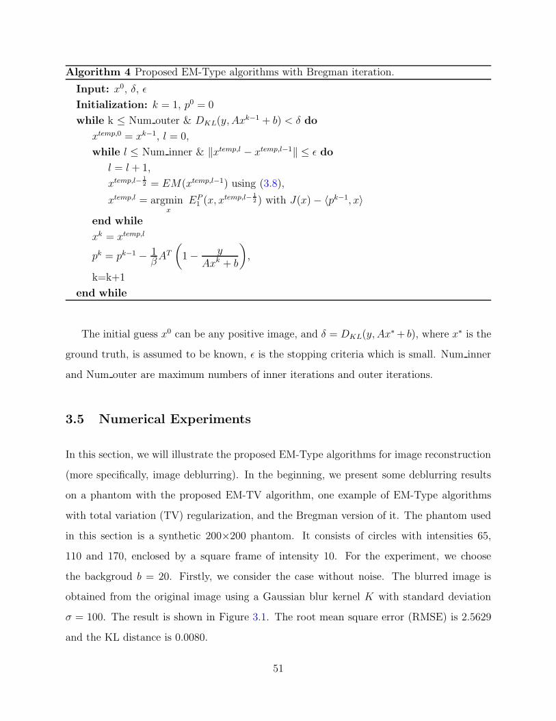
3.5 Numerical Experiments

In this section, we will illustrate the proposed EM-Type algorithms for image reconstruction

(more specifically, image deblurring). In the beginning, we present some deblurring results

on a phantom with the proposed EM-TV algorithm, one example of EM-Type algorithms

with total variation (TV) regularization, and the Bregman version of it. The phantom used

in this section is a synthetic 200×200 phantom. It consists of circles with intensities 65,

110 and 170, enclosed by a square frame of intensity 10. For the experiment, we choose

the backgroud b = 20. Firstly, we consider the case without noise. The blurred image is

obtained from the original image using a Gaussian blur kernel K with standard deviation

σ = 100. The result is shown in Figure 3.1. The root mean square error (RMSE) is 2.5629

and the KL distance is 0.0080.

51

(a) (b)

(c) (d)

0 20 40 60 80 100 120 140 160 180 2000

20

40

60

80

100

120

140

160

180

original imageblurred imagedeblurred image

(e)

Figure 3.1: (a) The orginal image u∗. (b) Blurred image K ∗u∗ using a Gaussian blur kernelK. (c) The deblurred image using the proposed EM-TV with Bregman iteration. (d) Thedifference between the deblurred image and the original image. (e) The lineouts of originalimage, blurred image and deblurred image in the middle row. Some parameters chosen areβ = 5, Num inner = 1 and Num outer = 10000.

52

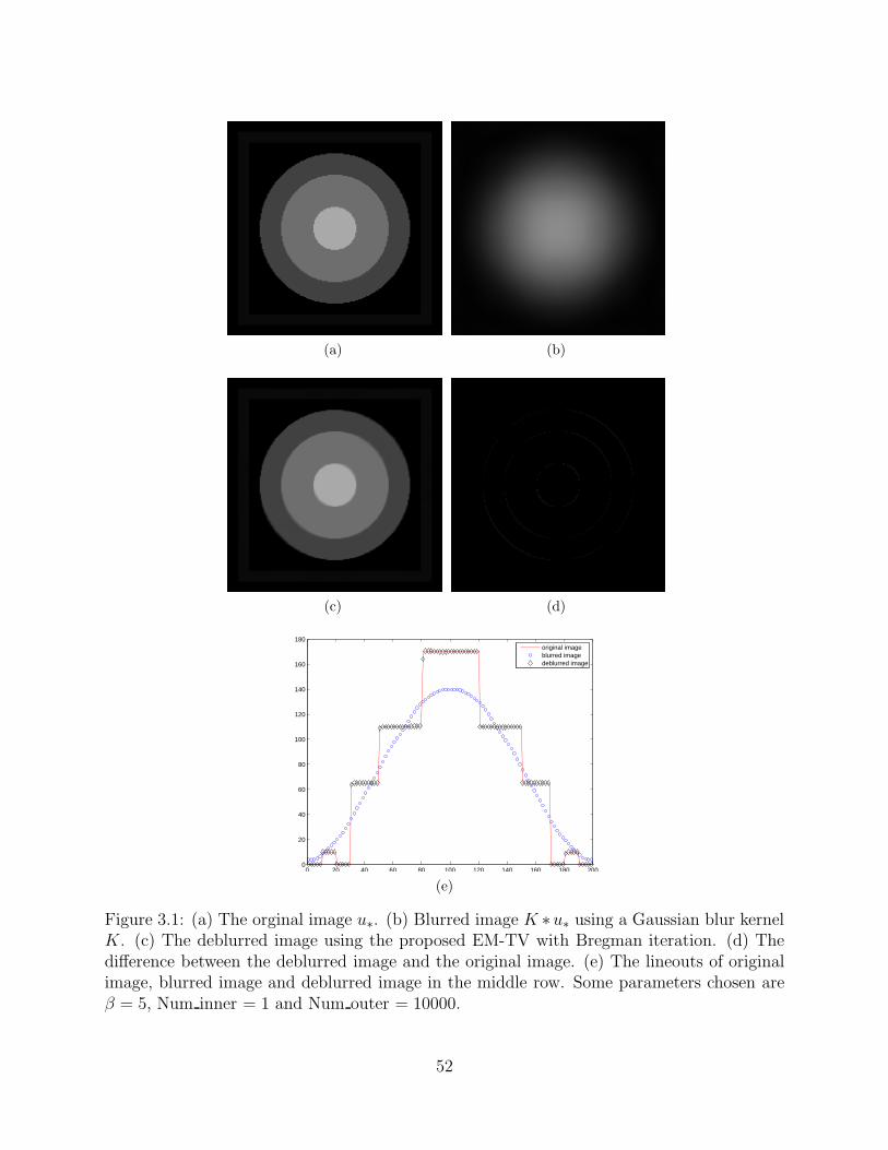
To illustrate the advantage of Bregman iterations, we show the comparison results of EM-

TV with different numbers of Bregman iterations in Figure 3.2. The RMSE for 3.2(a), 3.2(b)

and 3.2(c) are 11.9039, 5.0944 and 2.5339, respectively. The corresponding KL distances are

93.0227, 0.8607 and 0.0172, respectively.

(a) (b) (c)

0 10 20 30 40 50 60 70 80 90 1002

3

4

5

6

7

8

9

10

11

12

RMSE

(d)0 20 40 60 80 100 120 140 160 180 200

0

20

40

60

80

100

120

140

160

180

original imageblurred imageresult without Bregmanresult with Bregman

(e)

Figure 3.2: (a) The result without Bregman iteration. (b) The result with 25 Bregmaniterations. (c) The result with 100 Bregman iterations. (d) The plot of RMSE versusBregman iterations. (e) The lineouts of original image, blurred image, the results with andwithout Bregman iterations. Some parameters chosen are β = 0.001, Num inner = 100 andNum outer = 100.

How to choose a good parameter β is important for algorithms without Bregman iter-

ation because it balances the regularization and data fidelity, while it is not sensitive for

algorithms with Bregman iteration. For this experiment, though β is not chosen to be op-

53

timal, the results of Bregman iteration show that we can still obtain a good result after

several iterations. From the lineouts we can see that the result with Bregman iteration fits

the original image very well.

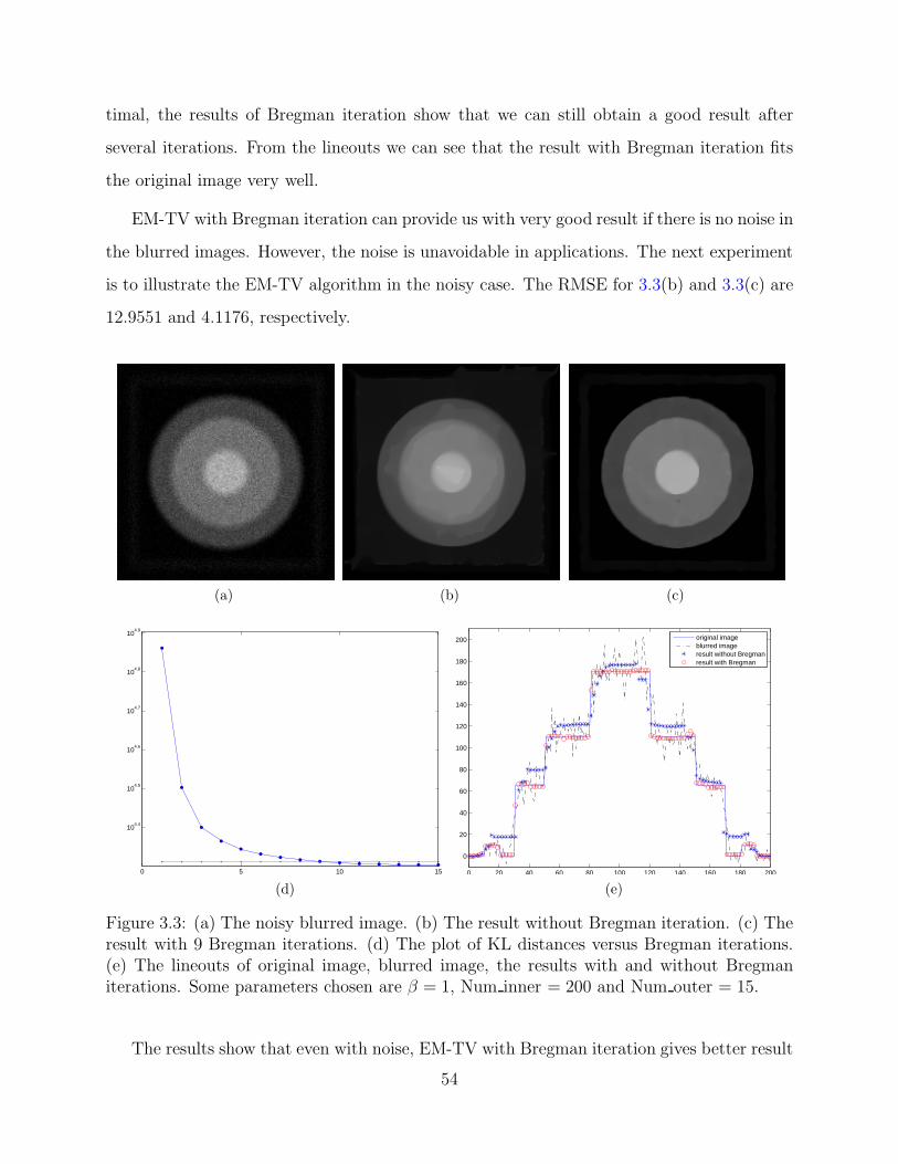
EM-TV with Bregman iteration can provide us with very good result if there is no noise in

the blurred images. However, the noise is unavoidable in applications. The next experiment

is to illustrate the EM-TV algorithm in the noisy case. The RMSE for 3.3(b) and 3.3(c) are

12.9551 and 4.1176, respectively.

(a) (b) (c)

0 5 10 15

104.4

104.5

104.6

104.7

104.8

104.9

(d)

0 20 40 60 80 100 120 140 160 180 200

0

20

40

60

80

100

120

140

160

180

200

original imageblurred imageresult without Bregmanresult with Bregman

(e)

Figure 3.3: (a) The noisy blurred image. (b) The result without Bregman iteration. (c) Theresult with 9 Bregman iterations. (d) The plot of KL distances versus Bregman iterations.(e) The lineouts of original image, blurred image, the results with and without Bregmaniterations. Some parameters chosen are β = 1, Num inner = 200 and Num outer = 15.

The results show that even with noise, EM-TV with Bregman iteration gives better result

54

than EM-TV without Bregman iteration.

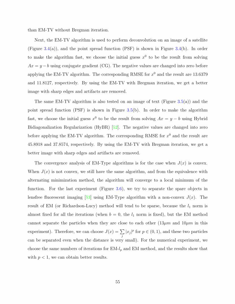
Next, the EM-TV algorithm is used to perform deconvolution on an image of a satellite

(Figure 3.4(a)), and the point spread function (PSF) is shown in Figure 3.4(b). In order

to make the algorithm fast, we choose the initial guess x0 to be the result from solving

Ax = y− b using conjugate gradient (CG). The negative values are changed into zero before

applying the EM-TV algorithm. The corresponding RMSE for x0 and the result are 13.6379

and 11.8127, respectively. By using the EM-TV with Bregman iteration, we get a better

image with sharp edges and artifacts are removed.

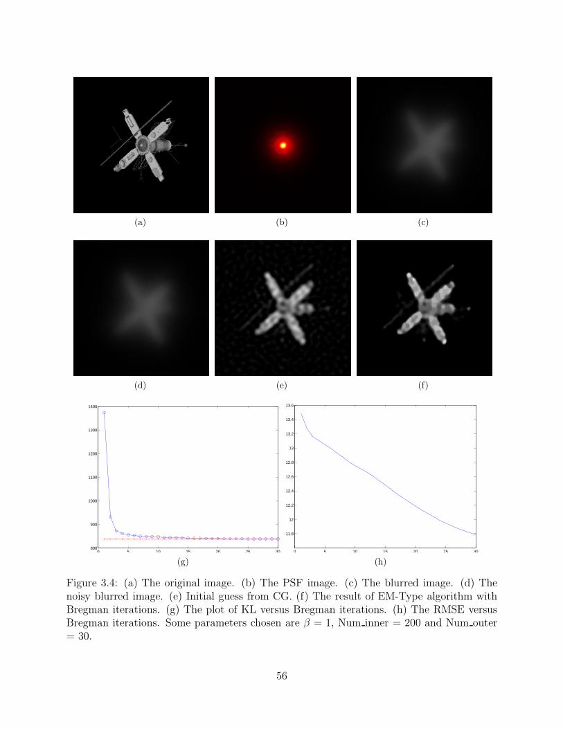
The same EM-TV algorithm is also tested on an image of text (Figure 3.5(a)) and the

point spread function (PSF) is shown in Figure 3.5(b). In order to make the algorithm

fast, we choose the initial guess x0 to be the result from solving Ax = y − b using Hybrid

Bidiagonalization Regularization (HyBR) [52]. The negative values are changed into zero

before applying the EM-TV algorithm. The corresponding RMSE for x0 and the result are

45.8918 and 37.8574, respectively. By using the EM-TV with Bregman iteration, we get a

better image with sharp edges and artifacts are removed.

The convergence analysis of EM-Type algorithms is for the case when J(x) is convex.

When J(x) is not convex, we still have the same algorithm, and from the equivalence with

alternating minimization method, the algorithm will converge to a local minimum of the

function. For the last experiment (Figure 3.6), we try to separate the spare objects in

lensfree fluorescent imaging [53] using EM-Type algorithm with a non-convex J(x). The

result of EM (or Richardson-Lucy) method will tend to be sparse, because the l1 norm is

almost fixed for all the iterations (when b = 0, the l1 norm is fixed), but the EM method

cannot separate the particles when they are close to each other (13µm and 10µm in this

experiment). Therefore, we can choose J(x) =∑

j

|xj|p for p ∈ (0, 1), and these two particles

can be separated even when the distance is very small). For the numerical experiment, we

choose the same numbers of iterations for EM-lp and EM method, and the results show that

with p < 1, we can obtain better results.

55

(a) (b) (c)

(d) (e) (f)

0 5 10 15 20 25 30800

900

1000

1100

1200

1300

1400

(g)

0 5 10 15 20 25 30

11.8

12

12.2

12.4

12.6

12.8

13

13.2

13.4

13.6

(h)

Figure 3.4: (a) The original image. (b) The PSF image. (c) The blurred image. (d) Thenoisy blurred image. (e) Initial guess from CG. (f) The result of EM-Type algorithm withBregman iterations. (g) The plot of KL versus Bregman iterations. (h) The RMSE versusBregman iterations. Some parameters chosen are β = 1, Num inner = 200 and Num outer= 30.

56

(a) (b) (c)

(d) (e) (f)

50 100 150 200 25082

84

86

88

90

92

94

96

98

100

102

(g)

0 50 100 150 200 25038

39

40

41

42

43

44

45

46

47

48

(h)

Figure 3.5: (a) The original image. (b) The PSF image. (c) The blurred image. (d) Thenoisy blurred image. (e) Initial guess from HyBR. (f) The result of EM-Type algorithm withBregman iterations. (g) The plot of KL versus Bregman iterations. (h) The RMSE versusBregman iterations. Some parameters chosen are β = 10−5, Num inner = 10 and Num outer= 250.

57

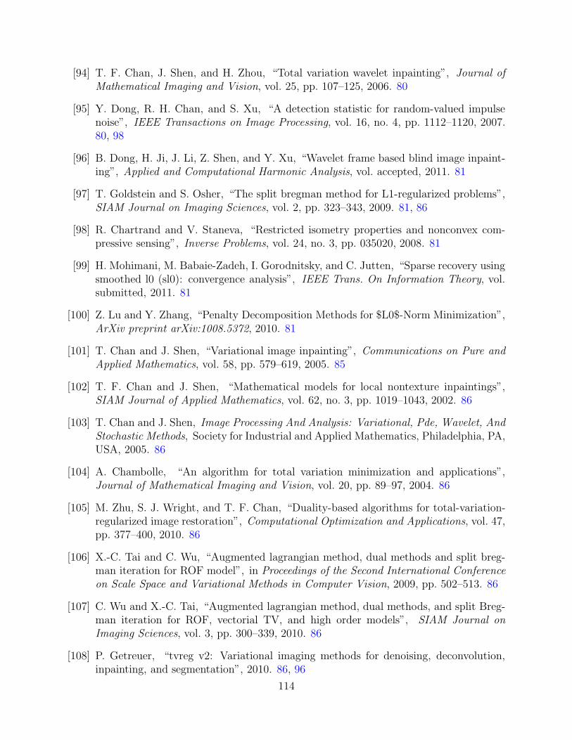
(a) 30µm (b) 21µm (c) 18µm (d) 13µm (e) 10µm

(f) 30µm (g) 21.6µm (h) 18.1µm (i) 12.4µm (j) 9µm

(k) 30µm (l) 21.6µm (m) NA (n) NA (o) NA

Figure 3.6: Top row shows raw lensfree fluorescent images of different pairs of particles. Thedistances betweens thes two particles are 30µm, 21µm, 18µm, 13µm and 9µm, from left toright. Middle row shows the results of EM-Type algorithm with p = 0.5. Bottom row showsthe results for EM (or Richardson-Lucy) method.

3.6 Conclusion

In this chapter, we proposed general robust EM-Type algorithms for image reconstruction

with background emission when the measured data is corrupted by Poisson noise: iteratively

performing EM and regularization in the image domain. The convergence of these algorithms

is proved in several ways. For the case without regularization, the KL distance to the limit of

the sequence of iterations is decreasing. The problem with regularization will lead to contrast

reduction in the reconstructed images. Therefore, in order to improve the contrast, we

suggested EM-Type algorithms with Bregman iteration by applying a sequence of modified

58

EM-Type algorithms. We have tested EM-Type algorithms with different J(x). With TV

regularization, this EM-TV algorithm can provide images with preserved edges and artifacts

are removed. When lp regularization is used, this EM-lp algorithm can be used to separate

sparse particles even when the distance is small, in which case the EM method can not do

a good job.

59

Part II

Adaptive Outlier Pursuit

60

CHAPTER 4

Adaptive Outlier Pursuit for Robust 1-Bit

Compressive Sensing

4.1 Introduction

The theory of compressive sensing (CS) enables reconstruction of sparse or compressible

signals from a small number of linear measurements relative to the dimension of the signal

space [54, 55, 56, 57, 58]. In this setting, we have

y = Φx, (4.1)

where x ∈ RN is the signal, Φ ∈ RM×N with M < N is an underdetermined measurement

system, and y ∈ RM is the set of linear measurements. It was demonstrated that K-sparse

signals, i.e., x ∈ ΣK where ΣK := x ∈ RN : ‖x‖0 := |supp(x)| ≤ K, can be reconstructed

exactly if Φ satisfies the restricted isometry property (RIP) [59]. It was also shown that

random matrices will satisfy the RIP with high probability if the entries are chosen according

to independent and identically distributed (i.i.d.) Gaussian distribution.

Classic compressive sensing assumes that the measurements are real valued and have

infinite bit precision. However, in practice, CS measurements must be quantized, i.e., each

measurement has to be mapped from a real value (over a potentially infinite range) to a

discrete value over some finite range, which will induce error in the measurements. The

quantization of CS measurements has been studied recently and several new algorithms were

proposed [60, 61, 62, 63, 64, 65].

Furthermore, for some real world problems, severe quantization may be inherent or pre-

61

ferred. For example, in analog-to-digital conversion (ADC), the acquisition of 1-bit measure-

ments of an analog signal only requires a comparator to zero, which is an inexpensive and

fast piece of hardware that is robust to amplification of the signal and other errors, as long

as they preserve the signs of the measurements, see [5, 66]. In this paper, we will focus on

the CS problem when a 1-bit quantizer is used.

The 1-bit compressive sensing framework proposed in [5] is as follows. Measurements of

a signal x ∈ RN are computed via

y = A(x) := sign(Φx). (4.2)

Therefore, the measurement operator A(·) is a mapping from RN to the Boolean cube 1

BM := −1, 1M . We have to recover a signal x ∈∑∗

K := x ∈ SN−1 : ‖x‖0 ≤ K where

SN−1 := x ∈ RN : ‖x‖2 = 1 is the unit hyper-sphere of dimension N . Since the scale

of the signal is lost during the quantization process, we can restrict the sparse signals to

be on the unit hyper-sphere. Jacques et al. provided two flavors of results for the 1-bit CS

framework [67]: 1) a lower bound is provided on the best achievable performance of this 1-bit

CS framework, and if the elements of Φ are drawn randomly from i.i.d. Gaussian distribution

or its rows are drawn uniformly from the unit sphere, then the solution will have bounded

error on the order of the optimal lower bound; and 2) a condition on the mapping A, binary

ǫ-stable embedding (BǫSE), that enables stable reconstruction is given to characterize the

reconstruction performance even when some of the measurement signs have changed (e.g.,

due to noise in the measurements).

Since this problem was introduced and studied by Boufounos and Baraniuk in 2008 [5], it

has been studied by many people and several algorithms have been developed [5, 67, 68, 69,

70, 71, 72]. Binary iterative hard thresholding (BIHT) [67] is shown to perform better than

other algorithms such as matching sign pursuit (MSP) [68] and restricted-step shrinkage

(RSS) [70] in reconstruction error as well as consistency, see [67] for more details. The

experiment in [67] shows that the one-sided ℓ1 objective (BIHT) performs better when there

1Generally, the M -dimensional Boolean cube is defined as 0, 1M . Without loss of generality, we use−1, 1M instead.

62

are only a few errors, and the one-sided ℓ2 objective (BIHT-ℓ2) performs better when there

are significantly more errors, which implies that BIHT-ℓ2 is useful when the measurements

contain significant noise that might cause a large number of sign flips.

In practice, there will always be noise in the measurements during acquisition and trans-

mission, therefore, a robust algorithm for 1-bit compressive sensing when the measurements

flip their signs is strongly needed. One possible way to build this robust algorithm is to

introduce an outlier detection technique.

There are many applications where the accurate detection of outliers is needed. For

example, when an image is corrupted by random-valued impulse noise, the corrupted pixels

are useless in image denoising. There are some methods (e.g., adaptive center-weighted

median filter (ACWMF) [4]) for detecting the damaged pixels. But these methods will miss

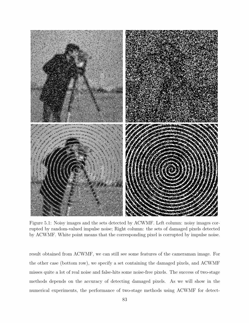
quite a lot of real noise and false-hit some noise-free pixels when the noise level is high. In

[73], we proposed a method to adaptively detect the noisy pixels and restore the image with

ℓ0 minimization. Instead of detecting the damaged pixels before recovering the image, we

iteratively restore the image and detect the damaged pixels. This idea works really well for

impulse noise removal. In this 1-bit compressive sensing framework, when there is a sign

flip in one measurement, this measurement will worsen the reconstruction performance. If

we can detect all the measurements with sign flips, then we can change the signs for these

measurements and improve the reconstruction performance a lot. However, it is much more

difficult than detecting impulse noise and there is no method for detecting sign flips, but

we can still utilize the idea in [73] to adaptively find the sign flips. In this chapter, we will

introduce a method for robust 1-bit compressive sensing which can detect the sign flips and

reconstruct the signals with very high accuracy even when there are a large number of sign

flips.

This chapter is organized as follows. We will introduce several algorithms for recon-

structing the signal and detecting the sign flips in section 4.2. Section 4.3 studies the case

when the noise information is not given. The performance of these algorithms is illustrated

in section 4.4 with comparison to BIHT and BIHT-ℓ2. We will end this work by a short

conclusion.

63

4.2 Robust 1-bit Compressive Sensing using

Adaptive Outlier Pursuit

Binary iterative hard thresholding (BIHT or BIHT-ℓ2) in [67] is the algorithm for solving

minimizex

M∑

i=1

φ(yi, (Φx)i)

subject to: ‖x‖2 = 1, ‖x‖0 ≤ K,

(4.3)

where φ is the one-sided ℓ1 (or ℓ2) objective:

φ(x, y) =

0, if x · y > 0,

|x · y| (or |x · y|2/2), otherwise.(4.4)

The high performance of BIHT is demonstrated when all the measurements are noise-free.

However when there are a lot of sign flips, the performance of BIHT and BIHT-ℓ2 is worsened

by the noisy measurements. There is no method to detect the sign flips in the measurements,

but adaptively finding the sign flips and reconstructing the signals can be combined together

as in [73] to obtain better performance.

Let us assume firstly that the noise level (the ratio of the number of sign flips over

the number of measurements for 1-bit compressive sensing) is provided. Based on this

information, we can choose a proper integer L such that at most L elements of the total

measurements are wrongly detected (having sign flips). For measurements y ∈ −1, 1M ,

Λ ∈ RM is a binary vector denoting the “correct” data:

Λi =

1, if yi is “correct”,

0, otherwise.(4.5)

According to the assumption, we haveM∑

i=1

(1− Λi) ≤ L.

Introducing Λ into the old problem solved by BIHT, we have the following new problem

64

with unknown variables x and Λ:

minimizex,Λ

M∑

i=1

Λiφ(yi, (Φx)i)

s.t.M∑

i=1

(1− Λi) ≤ L,

Λi ∈ 0, 1 i = 1, 2, · · · ,M,

‖x‖2 = 1, ‖x‖0 ≤ K.

(4.6)

The above model can also be interpreted in the following way. Let us consider the noisy

measurements y as the signs of Φx with additive unknown noise n, i.e., y = sign(Φx + n).

Though the binary measurement is robust to noise as long as the sign does not change,

there exist some ni’s such that the corresponding measurements change. In our problem,

only a few measurements are corrupted, and only these corresponding ni’s are important.

Therefore, n can be considered as sparse noise with nonzero entries at these locations, and

we have to recover the signal x from sparsely corrupted measurements [74, 75], even when

the measurements are acquired by taking the signs of Φx+ n. This equivalent problem is

minimizex,n

M∑

i=1

φ(yi, (Φx)i + ni)

s.t. ‖n‖0 ≤ L,

‖x‖2 = 1, ‖x‖0 ≤ K.

(4.7)

The equivalence is described in the appendix at the end of this chapter.

The problem defined in (4.6) is non-convex and has both continuous and discrete vari-

ables. It is difficult to find (x,Λ) together, thus we use an alternating minimization method,

which separates the energy minimization over x and Λ into two steps:

• Fix Λ and solve for x:

minimizex

M∑

i=1

Λiφ(yi, (Φx)i)

s.t. ‖x‖2 = 1, ‖x‖0 ≤ K.

(4.8)

This is the same as (4.3) with revised Φ and y. We only need to use the ith rows of Φ

65

and y where Λi = 1.

• Fix x and update Λ:

minimizeΛ

M∑

i=1

Λiφ(yi, (Φx)i)

s.t.M∑

i=1

(1− Λi) ≤ L,

Λi ∈ 0, 1 i = 1, 2, · · · ,M.

(4.9)

This problem is to chooseM−L elements with least sum fromM elements φ(yi, (Φx)i)Mi=1.

Given an x estimated from (4.8), we can update Λ in one step:

Λi =

0, if φ(yi, (Φx)i) ≥ τ,

1, otherwise,(4.10)

where τ is the Lth largest term of φ(yi, (Φx)i)Mi=1. If the Lth and (L + 1)th largest

terms are equal, then we can choose any Λ such that∑M

i=1 Λi = M − L and

mini,Λi=0

φ(yi, (Φx)i) ≥ maxi,Λi=1

φ(yi, (Φx)i).

Since for each step, the updated Λ identifies the outliers, this method is named as adaptive

outlier pursuit (AOP). When L = 0, this is exactly the BIHT proposed in [67]. Our algorithm

is as follows:

66

Algorithm 5 AOP

Input: Φ ∈ RM×N , y ∈ −1, 1M , K > 0, L ≥ 0, α > 0, Miter > 0Initialization: x0 = ΦTy/‖ΦTy‖, k = 0, Λ = 1 ∈ RM , Loc = 1 : M , tol = inf, TOL= inf.while k ≤ Miter and L ≤ tol do

Compute βk+1 = xk + αΦ(Loc, :)T (y(Loc)− sign(Φ(Loc, :)xk)).Update xk+1 = ηK(β

k+1),Set tol = ‖y −A(xk+1)‖0.if tol ≤TOL then,

Compute Λ with (4.10).Update Loc to be the location of 1-entries of Λ.Set TOL = tol.

end ifk = k + 1.

end whilereturn xk/‖xk‖.

ηK(v) computes the bestK-term approximation of v by thresholding. Since yi ∈ −1, 1,once we find the locations of the errors, instead of deleting these data, we can also “cor-

rect” them by flipping their signs. Hence x can also be updated with Φ and these new

measurements. This algorithm with changing signs is called AOP with flips.

Remark: Similar to BIHT-ℓ2, we can also choose the one-sided ℓ2 objective instead of

the ℓ1 objective and obtain two other algorithms.

4.3 The case with L unknown

In the previous section, we assume that L, the number of corrupted measurements, is known

in advance. However in real world applications there are cases when no pre-knowledge about

the noise is given. If L is chosen smaller or larger than the true value, the performance of

these algorithms will get worse. As shown numerically in section 4.4, when L is less than

the true value, even if the L detections are completely correct, some sign flips still remain

in the measurements. On the other hand, some correct measurements will be lost if L is too

large, and the problem will have more solutions if the number of total measurements is not

large enough, which will affect the accuracy of the algorithm. Therefore, in this scenario we

67

have to apply an L detection skill to find an L which is not far from the true value.

When no noise information is given, the following procedure can be applied to predict L.

The first-phase preparation is to do extensive experiments on simulated data with known L

and record the Hamming distances between A(x) and noisy y of BIHT-ℓ2 and AOP. Here

we can simply use the results in our first experiment in section 4.4. The average of the

results describes nicely the behavior of these two algorithms at different noise levels. Hence

a formula can be derived to predict the Hamming distance of AOP based on the results

obtained by BIHT-ℓ2. This could be a fair initial guess for the noise level, and we can derive

an L based on the result, labeled as L0. Then we calculate Lt = ‖A(x)−y‖0 using the result

x gained by AOP with L0 as the input for L. If Lt is greater than L0, which means that L0

is too small while Lt is too large, we set Lt as the upper bound Lmax and L0 as the lower

bound Lmin. Otherwise, if Lt is smaller than or equal to L0, which means L0 may be too

large, we use µLt (0 < µ < 1) as the new L0 to look for new Lt. We will keep doing this

until Lt is greater than L0. Then the previous L0 is defined as the upper bound Lmax and

the new L0 is defined as the lower bound Lmin. This is just one method for finding lower

and upper bounds for L, and there are certainly other possible ways to decide the bounds.

Then we use the bisection method to find a better L. The mean of Lmax and Lmin (Lmean) is

then used as input to derive Lt with AOP. If Lt is greater than Lmean, we update Lmin with

Lmean. Otherwise, Lmean is set as Lmax. This bisection method is applied to update these

two bounds until Lmax − Lmin ≤ 1. The final Lmin is our input L.

4.4 Numerical Results

In this section we use several numerical experiments to demonstrate the effectiveness of AOP

algorithms. Here AOP is implemented in the following four ways: 1) AOP with one-sided ℓ1

objective (AOP); 2) AOP with flips and one-sided ℓ1 objective (AOP-f); 3) AOP with one-

sided ℓ2 objective (AOP-ℓ2); and 4) AOP with flips and one-sided ℓ2 objective (AOP-ℓ2-f).

The four algorithms, together with BIHT and BIHT-ℓ2, are studied and compared in the

following experiments.

68

The setup for our experiments is as follows. We first generate a matrix Φ ∈ RM×N whose

elements follow i.i.d. Gaussian distribution. Then we generate the original K-sparse signal

x∗ ∈ RN . Its non-zero entries are drawn from standard Gaussian distribution and then

normalized to have norm 1. y∗ ∈ −1, 1M is computed by A(x∗).

4.4.1 Noise levels test

In our first experiment, we set M = N = 1000, K = 10, and examine the performance

of these algorithms on data with different noise levels. Here in each test, we choose a few

measurements at random and flip their signs. The noise level is between 0% and 10% and

we assume it is known in advance. For each level, we perform 100 trials and record the

average signal-to-noise ratio (SNR), average reconstruction angular error for each recon-

structed signal x with respect to x∗, average Hamming error between A(x) and A(x∗), and

average Hamming distance between A(x) and the noisy measurements y. Here SNR is de-

noted by 10 log10(‖x‖2/‖x−x∗‖2), angular error is defined as arccos〈x, x∗〉/π, Hamming error

stands for ‖A(x) − A(x∗)‖0/M and the Hamming distance between A(x) and y, defined as

‖A(x)−y‖0/M , is used to measure the difference between A(x) and the noisy measurements

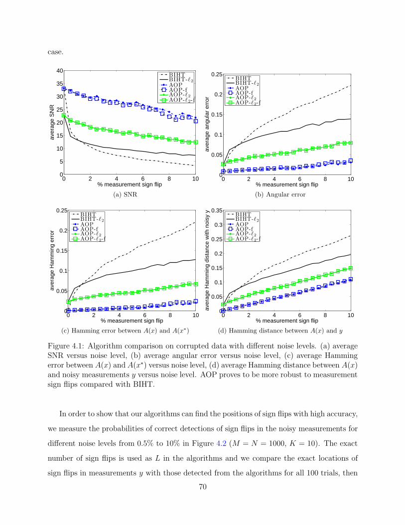
y. The results are depicted in Figure 4.1. The plots demonstrate that in these comparisons

four AOP algorithms outperform BIHT and BIHT-ℓ2 for all noise levels, significantly so when

more than 2% of the measurements are corrupted. Compared with BIHT, BIHT-ℓ2 tends to

give worse results when there are only a few sign flips in y and better results if we have high

noise level. This has been shown and studied in [67]. Of all the AOP series, AOP and AOP-f

give better results compared with AOP-ℓ2 and AOP-ℓ2-f. We can also see that there is a lot

of overlap between the results obtained by AOP and the ones acquired by AOP with flips,

especially when one-sided ℓ2 objective is used, the results are almost the same. Figure 4.1(d)

compares the average Hamming distances between A(x) and the noisy measurements y for

all algorithms. If the sign flips can be found correctly, then the Hamming distance between

A(x) and y should be equal to the noise level. The result shows that average Hamming

distances for AOP and AOP-f are slightly above the noise levels, which means that AOP

with one-sided ℓ1 objective performs better in consistency than other algorithms in noisy

69

case.

0 2 4 6 8 100

5

10

15

20

25

30

35

40

% measurement sign flip

aver

age

SN

R

BIHTBIHT-ℓ2

AOPAOP-fAOP-ℓ2

AOP-ℓ2-f

(a) SNR

0 2 4 6 8 100

0.05

0.1

0.15

0.2

0.25


aver

age

angu

lar

erro

r

BIHTBIHT-ℓ2

AOPAOP-fAOP-ℓ2

AOP-ℓ2-f

(b) Angular error

0 2 4 6 8 100

0.05

0.1

0.15

0.2

0.25


aver

age

Ham

min

g er

ror

BIHTBIHT-ℓ2

AOPAOP-fAOP-ℓ2

AOP-ℓ2-f

(c) Hamming error between A(x) and A(x∗)

0 2 4 6 8 100

0.05

0.1

0.15

0.2

0.25

0.3

0.35


aver

age

Ham

min

g di

stan

ce w

ith n

oisy

y

BIHTBIHT-ℓ2

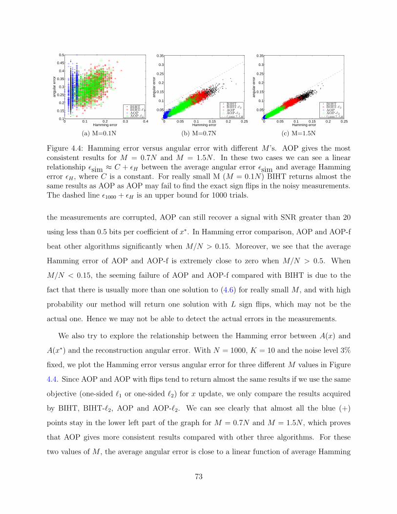
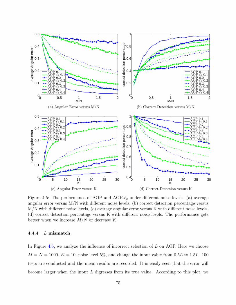
AOPAOP-fAOP-ℓ2

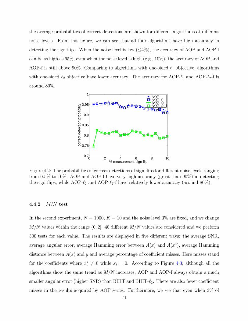
AOP-ℓ2-f

(d) Hamming distance between A(x) and y

Figure 4.1: Algorithm comparison on corrupted data with different noise levels. (a) averageSNR versus noise level, (b) average angular error versus noise level, (c) average Hammingerror between A(x) andA(x∗) versus noise level, (d) average Hamming distance between A(x)and noisy measurements y versus noise level. AOP proves to be more robust to measurementsign flips compared with BIHT.

In order to show that our algorithms can find the positions of sign flips with high accuracy,

we measure the probabilities of correct detections of sign flips in the noisy measurements for

different noise levels from 0.5% to 10% in Figure 4.2 (M = N = 1000, K = 10). The exact

number of sign flips is used as L in the algorithms and we compare the exact locations of

sign flips in measurements y with those detected from the algorithms for all 100 trials, then

70

the average probabilities of correct detections are shown for different algorithms at different

noise levels. From this figure, we can see that all four algorithms have high accuracy in

detecting the sign flips. When the noise level is low (≤4%), the accuracy of AOP and AOP-f

can be as high as 95%, even when the noise level is high (e.g., 10%), the accuracy of AOP and

AOP-f is still above 90%. Comparing to algorithms with one-sided ℓ1 objective, algorithms

with one-sided ℓ2 objective have lower accuracy. The accuracy for AOP-ℓ2 and AOP-ℓ2-f is

around 80%.

0 2 4 6 8 100.7

0.75

0.8

0.85

0.9

0.95

1


corr

ect d

etec

tion

prob

abili

ty

AOPAOP-fAOP-ℓ2

AOP-ℓ2-f

Figure 4.2: The probabilities of correct detections of sign flips for different noise levels rangingfrom 0.5% to 10%. AOP and AOP-f have very high accuracy (great than 90%) in detectingthe sign flips, while AOP-ℓ2 and AOP-ℓ2-f have relatively lower accuracy (around 80%).

4.4.2 M/N test

In the second experiment, N = 1000, K = 10 and the noise level 3% are fixed, and we change

M/N values within the range (0, 2]. 40 different M/N values are considered and we perform

300 tests for each value. The results are displayed in five different ways: the average SNR,

average angular error, average Hamming error between A(x) and A(x∗), average Hamming

distance between A(x) and y and average percentage of coefficient misses. Here misses stand

for the coefficients where x∗i 6= 0 while xi = 0. According to Figure 4.3, although all the

algorithms show the same trend as M/N increases, AOP and AOP-f always obtain a much

smaller angular error (higher SNR) than BIHT and BIHT-ℓ2. There are also fewer coefficient

misses in the results acquired by AOP series. Furthermore, we see that even when 3% of

71

0 0.5 1 1.5 2−5

0

5

10

15

20

25

30

35

40

M/N

aver

age

SN

R

BIHTBIHT-ℓ2

AOPAOP-fAOP-ℓ2

AOP-ℓ2-f

(a) SNR

0 0.5 1 1.5 20

0.05

0.1

0.15

0.2

0.25

0.3

0.35

0.4

M/N

aver

age

angu

lar

erro

r

BIHTBIHT-ℓ2

AOPAOP-fAOP-ℓ2

AOP-ℓ2-f

(b) Angular error

0 0.5 1 1.5 20

0.05

0.1

0.15

0.2

M/N

aver

age

Ham

min

g er

ror

BIHTBIHT-ℓ2

AOPAOP-fAOP-ℓ2

AOP-ℓ2-f

(c) Hamming distance between A(x) andA(x∗)

0 0.5 1 1.5 20

0.05

0.1

0.15

0.2

M/N

aver

age

Ham

min

g di

stan

ce w

ith n

oisy

y

BIHTBIHT-ℓ2

AOPAOP-fAOP-ℓ2

AOP-ℓ2-f

(d) Hamming error between A(x) and y

0 0.5 1 1.5 20

0.2

0.4

0.6

0.8

1

M/N

% c

oeffi

cien

t mis

ses

BIHTBIHT-ℓ2

AOPAOP-fAOP-ℓ2

AOP-ℓ2-f

(e) % coefficient misses

Figure 4.3: Algorithm comparison on corrupted data with different M/N . (a) average SNRversus M/N , (b) average angular error versus M/N , (c) average Hamming error betweenA(x) and A(x∗) versus M/N , (d) average Hamming distance between A(x) and y versusM/N , (e) average percentage of coefficient misses versus M/N . AOP yields a remarkableimprovement in reducing the Hamming and angular error and achieving higher SNR.

72

0 0.1 0.2 0.3 0.40.1

0.15

0.2

0.25

0.3

0.35

0.4

0.45

0.5

Hamming error

angu

lar

erro

r

BIHTBIHT-ℓ2

AOPAOP-ℓ2

(a) M=0.1N

0 0.05 0.1 0.15 0.2 0.250

0.05

0.1

0.15

0.2

0.25

0.3

0.35

Hamming error

angu

lar

erro

r

BIHTBIHT-ℓ2

AOPAOP-ℓ2

ǫ1000+ ǫH

(b) M=0.7N

0 0.05 0.1 0.15 0.2 0.250

0.05

0.1

0.15

0.2

0.25

0.3

0.35

Hamming error

angu

lar

erro

r

BIHTBIHT-ℓ2

AOPAOP-ℓ2

ǫ1000+ ǫH

(c) M=1.5N

Figure 4.4: Hamming error versus angular error with different M ’s. AOP gives the mostconsistent results for M = 0.7N and M = 1.5N . In these two cases we can see a linearrelationship ǫsim ≈ C + ǫH between the average angular error ǫsim and average Hammingerror ǫH , where C is a constant. For really small M (M = 0.1N) BIHT returns almost thesame results as AOP as AOP may fail to find the exact sign flips in the noisy measurements.The dashed line ǫ1000 + ǫH is an upper bound for 1000 trials.

the measurements are corrupted, AOP can still recover a signal with SNR greater than 20

using less than 0.5 bits per coefficient of x∗. In Hamming error comparison, AOP and AOP-f

beat other algorithms significantly when M/N > 0.15. Moreover, we see that the average

Hamming error of AOP and AOP-f is extremely close to zero when M/N > 0.5. When

M/N < 0.15, the seeming failure of AOP and AOP-f compared with BIHT is due to the

fact that there is usually more than one solution to (4.6) for really small M , and with high

probability our method will return one solution with L sign flips, which may not be the

actual one. Hence we may not be able to detect the actual errors in the measurements.

We also try to explore the relationship between the Hamming error between A(x) and

A(x∗) and the reconstruction angular error. With N = 1000, K = 10 and the noise level 3%

fixed, we plot the Hamming error versus angular error for three different M values in Figure

4.4. Since AOP and AOP with flips tend to return almost the same results if we use the same

objective (one-sided ℓ1 or one-sided ℓ2) for x update, we only compare the results acquired

by BIHT, BIHT-ℓ2, AOP and AOP-ℓ2. We can see clearly that almost all the blue (+)

points stay in the lower left part of the graph for M = 0.7N and M = 1.5N , which proves

that AOP gives more consistent results compared with other three algorithms. For these

two values of M , the average angular error is close to a linear function of average Hamming

73

error, which is predicted by BǫSE property in [67]. We also plot an empirical upper bound

ǫ1000 + ǫH for AOP defined in [67], where ǫ1000 is the largest angular error of AOP and ǫH

is the Hamming distance. Especially for the “under-sampled” case like M = 0.1N , none

of these algorithms are able to return consistent reconstructions, as we can see the points

scatter almost randomly over the domain. In this case the results obtained by BIHT stay

really close to those gained by AOP. As mentioned above, this is because AOP may not be

able to detect the exact sign flips in the noisy measurements when M is too small.

4.4.3 High noise levels

In this subsection, we study the performance of AOP and AOP-ℓ2 when a large number of

measurements are corrupted. Two settings are considered. In the first experiment, we fix

N = 1000, K = 10, and change theM/N ratio between 0.05 and 2. Four different noise levels

are considered from 0.1 to 0.4 and we record the average angular error and correct detection

probability from 100 tests. In the second setting, we fix M = 2000, N = 1000 and change K

from 1 to 30. Still, four noise levels are considered and the mean results from 100 tests are

recorded. From Figure 4.5 (a) and (b), we can see a similar trend for the behavior of angular

error and correct detection probability as we have discovered in Figure 4.3. According to

(c), (d), for all the noise levels the performance of these two algorithms tends to get worse as

K increases. We also have another interesting discovery that when the noise level is greater

than 0.2, AOP-ℓ2 turns out to be a better choice than AOP. This is because when the noise

level is extremely high, even with outlier detection technique, lots of sign flips remain in the

recovered measurements, and this new “noise level” is still relatively high. According to [67],

BIHT-ℓ2 outperforms BIHT when the measurements contain lots of sign flips. Therefore,

when the noise level is high enough, AOP-ℓ2 is considered as a better choice compared with

AOP.

74

0 0.5 1 1.5 20

0.1

0.2

0.3

0.4

0.5

M/N

aver

age

Ang

ular

err

or

AOP 0.1AOP-ℓ2 0.1AOP 0.2AOP-ℓ2 0.2AOP 0.3AOP-ℓ2 0.3AOP 0.4AOP-ℓ2 0.4

(a) Angular Error versus M/N

0 0.5 1 1.5 20

0.2

0.4

0.6

0.8

1

M/N

corr

ect d

etec

tion

perc

enta

ge


(b) Correct Detection versus M/N

0 5 10 15 20 25 300

0.1

0.2

0.3

0.4

0.5

K

aver

age

Ang

ular

err

or


(c) Angular Error versus K

0 5 10 15 20 25 300.4

0.5

0.6

0.7

0.8

0.9

1

K

corr

ect d

etec

tion

perc

enta

ge


(d) Correct Detection versus K

Figure 4.5: The performance of AOP and AOP-ℓ2 under different noise levels. (a) averageangular error versus M/N with different noise levels, (b) correct detection percentage versusM/N with different noise levels, (c) average angular error versus K with different noise levels,(d) correct detection percentage versus K with different noise levels. The performance getsbetter when we increase M/N or decrease K.

4.4.4 L mismatch

In Figure 4.6, we analyze the influence of incorrect selection of L on AOP. Here we choose

M = N = 1000, K = 10, noise level 5%, and change the input value from 0.5L to 1.5L. 100

tests are conducted and the mean results are recorded. It is easily seen that the error will

become larger when the input L digresses from its true value. According to this plot, we

75

know that in order to obtain good performance for our method, we should choose a proper

L as input.

0.5 1 1.50.05

0.1

0.15

0.2

0.25

L/Ltrue

aver

age

angu

lar

erro

r

(a) Angular Error

0.5 1 1.50.05

0.06

0.07

0.08

0.09

0.1

0.11

L/Ltrue

aver

age

Ham

min

g er

ror

(b) Hamming Error

Figure 4.6: The performance of AOP with different L inputs. L has to stay close to its truevalue in order to get good performance.

4.4.5 Unknown L

To show that our method works even when L is not given, we use the method described in

Section 4.3 to find an approximation of L, and compare the results of AOP with different

L’s. Here M = N = 1000, K = 10 are fixed, and 10 different noise levels (from 1% to

10%) are tested. Three inputs for L: the initial L0 predicted from the result of BIHT-ℓ2,

L obtained from bisection method, exact L, are used in AOP to obtain the results. The

following Figure 4.7 is depicted with the average results from 100 trials. Even with the

initial L0, the results are comparable to those with exact L, and the bisection method can

provide a better approximation for L with longer time for predicting L.

4.5 Conclusion

In this chapter, we propose a method based on adaptive outlier pursuit for robust 1-bit

compressive sensing. By iteratively detecting the sign flips in measurements and recovering

76

2 4 6 8 100

0.01

0.02

0.03

0.04

0.05


aver

age

angu

lar

erro

r

initial LL by bisectionexact L

(a) Angular error

2 4 6 8 100

0.02

0.04

0.06

0.08

0.1

0.12


aver

age

Ham

min

g di

stan

ce w

ith n

oisy

y

initial LL by bisectionexact L

(b) Hamming distance with noisy y

Figure 4.7: Comparison of results by different L’s at different noise levels from 1% to 10%.(a) average angular error versus noise level, (b) average Hamming distance between A(x)and noisy y versus noise level. By choosing appropriate L as the input, we can obtain theresults comparable to those with exact L.

the signals from “correct” measurements, this method can obtain better results in both

finding the noisy measurements and recovering the signals, even when there are a lot of

sign flips in the measurements. Four algorithms (AOP, AOP-f, AOP-ℓ2 and AOP-ℓ2-f) are

given based on this method, and the performance of these four algorithms is shown in the

numerical experiments. The algorithms based on one-sided ℓ1 objective (AOP and AOP-f)

have better performance compared to the other two algorithms (AOP-ℓ2 and AOP-ℓ2-f),

which are based on one-sided ℓ2 objective when the noise level is not high (less than 20%).

When the noise level is extremely high, AOP-ℓ2 is a better choice compared with AOP. In

addition, we propose a simple method to find a candidate for the number of sign flips L

when L is unknown and the numerical experiments show that the performance of AOP with

this inexact input L is comparable with that of exact L.

77

Appendix

In this appendix, we show the equivalence of problems (4.6) and (4.7). If (x, n) satisfies the

constraints of problem (4.7), we can define

Λi =

1, if ni = 0,

0, otherwise.(4.11)

Then we have φ(yi, (Φx)i+ni) = 0 if Λi = 0, as we can always find ni such that φ(yi, (Φx)i+

ni) = 0 for fixed x. If Λi = 1, we have ni = 0, thus φ(yi, (Φx)i+ni) = φ(yi, (Φx)i). Therefore,

problem (4.7) is equivalent to

minimizex,n

M∑

i=1

Λiφ(yi, (Φx)i)

s.t. ‖n‖0 ≤ L,

‖x‖2 = 1, ‖x‖0 ≤ K.

(4.12)

From the relation of Λ and n in (4.11), we know that the constraint ‖n‖0 ≤ L in the above

problem can be replaced with the constraint on Λ defined in (4.6). Therefore, problems (4.6)

and (4.7) are equivalent.

78

CHAPTER 5

Impulse Noise Removal

5.1 Introduction

Observed images are often corrupted by impulse noise during image acquisition and trans-

mission, caused by malfunctioning pixels in camera sensors, faulty memory locations in

hardware, or bit errors in transmission [76]. There are two common types of impulse noise:

salt-and-pepper impulse noise and random-valued impulse noise. Assume that the dynamic

range of an image is [dmin, dmax]. For images corrupted by salt-and-pepper impulse noise, the

noisy pixels can take only two values dmin and dmax, while for images corrupted by random-

valued impulse noise, the noisy pixels can take any random value between dmin and dmax.

In this work, the original unknown image u is defined on a domain Ω, and the observed

image f is modeled as

f =

Hu+ n1 x ∈ Ω1

n2 x ∈ Ωc1 := Ω\Ω1.

(5.1)

Here, n2 is the impulse noise, and n1 is the additive zero-mean Gaussian white noise. H

is the identity or a blurring operator. The subset Ωc1 of Ω denotes the region where the

information of Hu is missing. The problem is to find the true image u from observed f given

the operator H .

If Ωc1 is empty, there is no impulse noise, then we have f = Hu+ n1, which is an image

denoising (and deblurring) problem, and it has been extensively studied by both signal

processing researchers and mathematicians. If Ωc1 is not empty and known, this can be

considered as an image inpainting (and deblurring) problem.

79

Here, we will consider the last and most difficult case where Ωc1 is not empty and unknown.

The challenge of this problem is to restore the lost details, and remove the impulse noise

simultaneously. If n1 = 0, this problem is an impulse noise removal (and deblurring) problem

and if n1 6= 0 it becomes a mixed Gaussian impulse noise removal (and deblurring) problem.

There are already several types of approaches for solving this problem.

The first type of approaches treats n2 as outliers and uses the L1 norm in the fidelity

term to increase the robustness of inpainting to outliers [77, 78, 79, 80], and the problem is

to solve

minimizeu

∫

Ω

|Hu− f |dx+ J(u), (5.2)

where J(u) is a regularization on the true image u. There are many candidates for the

regularization J(u), some examples are Tikhonov regularization [81]; Geman and Reynolds’

half quadratic variational models [82]; Rudin, Osher and Fatemi’s total variation models

[2, 83]; and framelet based models [84, 85]. This approach does not need to find the damaged

pixels and performs well when there is only impulse noise. However, for the case of images

corrupted by mixed Gaussian impulse noise, the Gaussian noise is not treated properly.

The second type of approaches are the two-stage approach [86, 87, 88, 89, 85, 90], which

estimates the inpainting region Ωc1 before estimating u. In these approaches, the second

stage becomes a regular image inpainting (and deblurring) problem [91, 92, 93, 94]:

minimizeu

1

2

∫

Ω1

(Hu− f)2dx+ J(u). (5.3)

The success of these two-stage approaches relies on the accurate detection of Ωc1, e.g., adaptive

median filter (AMF) [3] is used to detect salt-and-pepper impulse noise, while adaptive

center-weighted median filter (ACWMF) [4] and rank-ordered logarithmic difference (ROLD)

[95] are utilized to detect random-valued impulse noise.

Though adaptive median filter can detect most pixels damaged by salt-and-pepper im-

pulse noise, it is more difficult to detect pixels corrupted by random-valued impulse noise

80

than salt-and-pepper impulse noise. Recently, by considering two different types of noise,

Dong et.al. [96] proposed a new method using framelets to remove random-valued impulse

noise plus Gaussian noise by solving

minimizeu,v

1

2

∫

Ω

(Hu+ v − f)2dx+ λ‖Wu‖1 +∫

Ω

|v|dx, (5.4)

where W is a transformation from the image to the framelet coefficients. Two unknowns u

(restored image) and v (noise) are introduced into this variational method, and their methods

can simultaneously find u and v using split Bregman iterations [97].

Dong et.al.’s method uses ℓ1 norm as a convex approximation of ℓ0 to make the result

v sparse, and keep the problem convex in the meantime. However, using non-convex op-

timization (ℓp when p < 1) has better performance than convex optimization in dealing

with sparsity, as shown in compressive sensing [98]. Even ℓ0 minimization and smoothed ℓ0

minimization are used in many algorithms [99, 100]. In this chapter, we will use ℓ0 instead

of ℓ1 minimization in the problem, and by using ℓ0, the problem in u and v is shown to

be equivalent to a problem in u and Ω1. Thus using alternating minimization algorithms,

it can be solved easily by alternately solving the image inpainting problem and finding the

damaged pixels.

The work is organized as follows. An introduction of ACWMF is given in section 5.2.

We will show in this section that ACWMF cannot detect the pixels corrupted by random-

valued impulse noise correctly. In section 5.3 and 5.4, we introduce our general methods

for removing impulse noise using two different treatments for ℓ0: I) the ℓ0 term is put in

the objective functional, II) the ℓ0 term is in the constraint. The algorithms for these two

methods and performances are similar. The convergence analysis is shown in section 5.5.

These algorithms will converge to coordinatewise minimum points. In addition, they will

converge to local minimum points (with probability one) with some modifications in the

algorithms. Some experiments are given in section 5.6 to show the efficiency of proposed

method for removing impulse noise and mixed Gaussian impulse noise. We will end this

work by a short conclusion section.

81

5.2 The Adaptive Center-Weighted Median Filter

In order to remove random-valued impulse noise, adaptive center-weighted median filter

(ACWMF) [4] is considered as a good method for detecting the damaged pixels when the

noise level is not too high. So the result of ACWMF is often utilized in two-stage ap-

proaches [88, 89, 85] to estimate the set of damaged pixels Ωc1.

If u is a noisy M-by-N (M × N) grayscale image, and ui,j is the gray level at pixel

(i, j) ∈ 1, · · · ,M × 1, · · · , N, the expression of the ACWMF filter is as follows:

y2ki,j = medianui−s,j−t, (2k) ⋄ ui,j| − h ≤ s, t ≤ h,

where (2h+ 1)× (2h+ 1) is the window size, and ⋄ represents the repetition operation. For

k = 0, 1, · · · , J − 1, where J = 2h(h+ 1), we can determine the differences dk = |y2ki,j − ui,j|.They satisfy the condition dk ≤ dk−1 for k ≥ 1. To determine if the considered pixel (i, j) is

noisy, a set of thresholds Tk is utilized, where Tk−1 > Tk for k = 1, · · · , J − 1. The output

of the filter is defined in the following manner:

uACWMF =

y0i,j, if dk > Tk for some k,

ui,j, otherwise.(5.5)

Usually, the window size is chosen as 3 × 3 (i.e., h = 1 and J = 4), four thresholds Tk

(k = 0, · · · , 3) are needed, and they are calculated as follows:

Tk = s ·MAD+ δk, (5.6)

MAD = median|ui−s,j−t − y1i,j| − h ≤ s, t ≤ h, (5.7)

where [δ0, δ1, δ2, δ3] = [40, 25, 10, 5] and 0 ≤ s ≤ 0.6.

The performance of ACWMF is demonstrated in Figure 5.1 on a 256x256 blurry camera-

man image when 25% of the pixels are corrupted by random-valued impulse noise. For the

first case (top row), the set having the corrupted pixels is chosen randomly, and from the

82

Figure 5.1: Noisy images and the sets detected by ACWMF. Left column: noisy images cor-rupted by random-valued impulse noise; Right column: the sets of damaged pixels detectedby ACWMF. White point means that the corresponding pixel is corrupted by impulse noise.

result obtained from ACWMF, we can still see some features of the cameraman image. For

the other case (bottom row), we specify a set containing the damaged pixels, and ACWMF

misses quite a lot of real noise and false-hits some noise-free pixels. The success of two-stage

methods depends on the accuracy of detecting damaged pixels. As we will show in the

numerical experiments, the performance of two-stage methods using ACWMF for detect-

83

ing damaged pixels is not good enough, and even worse than the methods using L1 fidelity

term. If the detection of damaged pixels can be updated during the image restoration with

increasing accuracy, then the performance will be better. In the next two sections, we will

provide two methods that iteratively update the detection of damaged pixels and restore the

images.

5.3 Blind Inpainting Models using ℓ0 Norm

5.3.1 Formulation

For a M×N image, Λ ∈ 0, 1M×N is a binary matrix denoting the undamaged pixels (pixels

not corrupted by impulse noise):

Λi,j =

1, if pixel (i, j) ∈ Ω1,

0, otherwise.(5.8)

We use PΛ(·) to represent the projection of an image onto a matrix supported by Λ:

PΛ(u)i,j =

0, if Λi,j = 0,

ui,j, if Λi,j = 1.(5.9)

Given a degraded image f , our objective is to estimate the damaged (or missing) pixels

and restore them. We propose the following model using ℓ0 minimization to solve this

problem:

minimizeu,v

1

2

∫

Ω

(Hu+ v − f)2dx+ λ1J(u) + λ2‖v‖0, (5.10)

where J(u) is the regularization term on the image, λ1 and λ2 are two positive parameters.

The parameter λ1 is dependent on the noise level of n1. The higher the noise level, the larger

the parameter should be. The parameter λ2 is dependent on the noise level of impulse noise.

The difference from Dong et.al.’s method is that ℓ1 norm is replaced by ℓ0. However, it is

84

difficult to solve this problem because of the ℓ0 term in the functional. We will show that

this problem in u and v is equivalent to a problem in u and Ω1, which is easy to solve.

Assume that (u∗, v∗) is the optimal solution to problem (5.10). When v∗i,j 6= 0, we have

v∗i,j = fi,j − (Hu∗)i,j. Therefore if we denote

Λi,j =

0, if vi,j 6= 0,

1, if vi,j = 0.(5.11)

then problem (5.10) is equivalent to

minimizeu,Λ

F1(u,Λ) ≡1

2

∑

i,j

Λi,j((Hu)i,j − fi,j)2 + λ1J(u) + λ2

∑

i,j

(1− Λi,j), (5.12)

which is a problem in u and Ω1, because each Ω1 corresponds to a unique binary matrix Λ.

Problem (5.12) can be solved easily by alternating minimization method, and the algorithm

for solving (5.12) is described below.

5.3.2 Algorithm

The objective function defined in (5.12) is non-convex and has both continuous and discrete

variables. It is still difficult to solve it in the pair (u,Λ), but we can use alternating min-

imization method, which separates the energy minimization over u and Λ into two steps.

For solving the problem in u with Λ fixed, it is a convex optimization problem for image

inpainting and finding Λ with u fixed is a combinatorial optimization problem, which can be

solved in one step. These two subproblems are

1) Finding u: Given an estimate of the support matrix Λ, the minimization over u is just

an image inpainting (and deblurring) problem [101]:

minimizeu

1

2

∫

Ω1

(Hu− f)2dx+ λ1J(u). (5.13)

There are many existing methods for solving this problem.

85

2) Finding Λ: Given an estimate of the image u, the minimization over Λ becomes:

minimizeΛ

1

2

∑

i,j

Λi,j((Hu)i,j − fi,j)2 − λ2

∑

i,j

Λi,j. (5.14)

Since this minimization problem of Λ is separable, it can be solved exactly in only one step:

Λi,j =

0 if ((Hu)i,j − fi,j)2 /2 > λ2,

0 or 1 if ((Hu)i,j − fi,j)2 /2 = λ2,

1 if ((Hu)i,j − fi,j)2 /2 < λ2.

(5.15)

Therefore, the proposed algorithm for blind inpainting with ℓ0 minimization is iteratively

finding u and Λ. If the regularization J(·) is chosen to be total variation, the detailed

algorithm is described below.

5.3.3 TV Blind Inpainting

If the regularization for the image u is the total variation, H is the identity operator and

the noise n1 is zero-mean Gaussian white noise, then problem (5.12) becomes

minimizeu,Λ

F1(u,Λ) ≡∑

i,j

1

2Λi,j(ui,j − fi,j)

2 + λ1

∫

Ω

|∇u|+ λ2

∑

i,j

(1− Λij). (5.16)

The step for finding u is

minimizeu

∑

i,j

1

2Λi,j(ui,j − fi,j)

2 + λ1

∫

Ω

|∇u|, (5.17)

which is the famous TV inpainting model [102, 103]. Numerous algorithms proposed for

solving TV denoising problem can be adopted to solve this TV inpainting problem with

some necessary modifications. Some examples are algorithms based on duality [104, 105],

augmented Lagrangian methods [106, 107], and split Bregman iterations [97, 108].

The algorithm for total variation blind inpainting is described below, the initial Λ0 is

chosen by the methods for detecting the impulse noise (AMF for salt-and-pepper impulse

86

noise and ACWMF for random-valued impulse noise). Usually three iterations are sufficient,

as shown in the experiments.

Algorithm 6 Proposed total variation blind inpainting algorithm.

Input: f , λ1, λ2, Λ0, ǫ

Initialization: k = 1.while k < 2 or F1(u

k,Λk)− F1(uk−1, λk−1) > ǫ do

Obtain uk by solving (5.17),Obtain Λk by (5.15).k = k + 1.

end while

5.4 Blind Inpainting Using Adaptive Outlier Pursuit

In the previous section, we proposed a method for blind inpainting by putting a ℓ0 term in

the objective functional, which can be solved by iteratively updating the set Λ and restoring

the image. Instead of putting the ℓ0 term in the objective functional, we can also put a

constraint on ‖v‖0, which will be equivalent to a constraint on∑

i,j Λi,j. This technique

has been applied to robust 1-bit compressive sensing where there are sign flips in the binary

measurements belonging to −1, 1 [109]. We proposed an algorithm, named adaptive outlier

pursuit (AOP), which can adaptively find the sign flips and reconstruct the signal by using

other measurements assumed to be correct. Since images corrupted by impulse noise can

also be considered as sparsely corrupted measurements, the same idea can be applied to

impulse noise (and mixed Gaussian impulse noise) removal by iteratively finding the pixels

corrupted by impulse noise and recovering the image using the other pixels.

Let us assume that the number of pixels corrupted by impulse noise is bounded above by

L, this can be obtained from the noise level of impulse noise. Therefore, the new problem is

minimizeu,v

12

∫

Ω(Hu+ v − f)2dx+ λ1J(u),

subject to ‖v‖0 ≤ L(5.18)

87

Similarly, we have the equivalent form in (u,Λ), which is

minimizeu,Λ

F2(u,Λ) ≡∑

i,j12Λi,j((Hu)i,j − fi,j)

2 + λ1J(u),

subject to∑

i,j(1− Λi,j) ≤ L, Λi,j ∈ 0, 1.(5.19)

This problem can also be solved iteratively as in previous section.

The u-subproblem is the same as the previous one, and the Λ-subproblem is slightly

different. In order to update Λ, we have to solve

minimizeΛ

∑

i,j((Hu)i,j − fi,j)2/2

subject to∑

i,j(1− Λi,j) ≤ L,Λi,j ∈ 0, 1.(5.20)

This problem is to choose M × N − L elements with least sum from M × N elements

((Hu)i,j − fi,j)2/2M,N

i=1,j=1. Given an u estimated from (5.17), we can update Λ in one step:

Λi,j =

0, if ((Hu)i,j − fi,j)2/2 ≥ λ2,

1, if ((Hu)i,j − fi,j)2/2 < λ2,

(5.21)

where λ2 is the Lth largest term of ((Hu)i,j−fi,j)

2/2M,Ni=1,j=1. If the L

th and (L+1)th largest

terms are equal, then we can choose any binary matrix Λ such that∑

i,j Λi,j = M ×N − L

and

mini,j,Λi,j=0

((Hu)i,jfi,j)2/2 ≥ max

i,j,Λi,j=1((Hu)i,j − fi,j)

2/2. (5.22)

The algorithm for total variation blind inpainting using AOP is described below.

Algorithm 7 Proposed total variation blind inpainting using AOP.

Input: f , λ1, L, Λ0, ǫ

Initialization: k = 1.while k < 2 or F2(u

k,Λk)− F2(uk−1, λk−1) > ǫ do

Obtain uk by solving (5.17),Obtain Λi by (5.21).k = k + 1.

end while

88

The difference between these two algorithms is the Λ-subproblem, the threshold λ2 is

fixed for algorithm 6, while λ2 is changing for AOP. AOP can be considered as one special

case of algorithm 6 with changing λ2. However the performance of these two algorithms is

similar, and the parameter L is easier to obtain than λ2. So we will only use algorithm 7 for

numerical experiments.

These two algorithms are both for the case where H is the identity, and there is no

blurring in the observed image. In order to show that our idea can be applied to other

two-stage approaches easily, we will introduce in the next subsection a method for dealing

with the case when H is a blurring operator using framelet.

5.4.1 Framelet-Based Deblurring

Though total variation (TV) is popular for regularization in recent years as it preserves edges,

its limitation is that TV-based regularization can not preserve the details and textures very

well in the regions of complex structures due to the stair-casing effects [110]. Therefore,

framelet-based algorithms are introduced in [84, 85] for impulse noise removal. In [85], itera-

tive framelet-based approximation/sparsity deblurring algorithm (IFASDA) and accelerated

algorithm of IFASDA (Fast IFASDA) are proposed to deblur images corrupted by impulse

plus Gaussian noise. They both have two steps, the first step is to apply AMF or ACWMF

on f to estimate the set Ωc1; the second step is deblurring the image using framelet from

PΛ(f).

The energy functional to be minimized is

E(u) := ‖φ(PΛ(Hu− f))‖1 + λ‖OwHu‖1, (5.23)

where OwH := [w1O21 w2OT

2 · · · w17OT17]

T and φ(x) = ηx2

η+|x|. Ok17k=0 are the matrix repre-

sentations of the tight framelet filters τk17k=0 under a proper boundary condition [111] (see

Section III in [85] for the tight framelet filters O and weight w). In addition a matrix OH is

89

formed by stacking the matrices Ok, 1 ≤ k ≤ 17 together, that is

OH = [O21 OT

2 · · · OT17]

T . (5.24)

Associated with the matrix OH and a diagonal matrix

Γ := diag(· · · , γl, · · · ), γl ≥ 0, (5.25)

the shrinkage function ShΓ : RM×N → RM×N is defined as follow:

ShΓ(f) := OT0 O0f +OT

H · shrink(OHf,Γ) (5.26)

where shrink is the componentwise thresholding operator

shrink(x,Γ)[l] = sign(x[l]) max|x[l]| − γl, 0. (5.27)

The algorithm is

un+1 = ShΓn(un − βn∇Jn(u

n)) (5.28)

where

Jn(y) := ‖φn(PΛ(Hy − f))‖1 + λn‖OwHy‖1, (5.29)

with

φn(x) =ηnx

2

ηn + |x| . (5.30)

The ACWMF can not estimate the set Ω1c perfectly, especially when noise level is high

and two types of impulse noise are present, thus frequently updating the set is necessary.

90

The new constrainted optimization problem using AOP is

minimizeu,Λ

‖φ(PΛ(Hu− f))‖1 + λ‖OwHu‖1

subject to:∑

i,j(1− Λi,j) ≤ K.

If alternating minimizing method is utilized, the first step for finding u is the same as

IFASDA, and the second step for updating Ω1 is very easy to find from (5.21). The modified

IFASDA algorithm Ada IFASDA is shown below:

Algorithm 8 Proposed framelet-based deblurring algorithm (Ada IFASDA).

Input: f , L, Λ,for k = 1, 2, · · · , do

Estimate ηk, βk, λk, Γk.Compute uk+1.Stop if uk+1 meets a stopping criteriaif mod(k,5)=0 then

Obtain Λ by (5.21).end ifk = k + 1.

end for

Here, the input Λ is obtained from ACWMF. In fact, we do not need to wait until the

step for finding u converges, several iterations in IFASDA are sufficient for the full algorithm

to converge. We choose to update the set Ω1c for every five iterations in IFASDA.

Similarly, Fast IFASDA can also be modified into Ada Fast IFASDA by adding the steps

for updating Ω1c every five iterations in Fast IFASDA.

5.5 Convergence Analysis

First of all, we will show that the constraint Λi,j ∈ 0, 1 in (5.12) and (5.19) can be

replaced by the relaxed constraint Λi,j ∈ [0, 1]. Because for every fixed u, we can always find

a minimum point of F1(u,Λ) (or F2(u,Λ)) satisfying the constraint Λi,j ∈ 0, 1. Therefore,for any local minimum of F1(u,Λ) (or F2(u,Λ)) with the relaxed constraint, we can find

a corresponding Λ satisfying the unrelaxed constraint such that the local minimum is the

91

same.

In this section, we establish some convergence results for these two algorithms. We

will show that the algorithm will stop in finite steps, and the output is a coordinatewise

minimum point of F1(u,Λ) (or F2(u,Λ)) with relaxed constraint Λi,j ∈ [0, 1]. In addition,

we can modify a little bit the algorithm and the output will be a local minimum point (with

probability one).

Let us define a new function combining F1(u,Λ) and F2(u,Λ) as follows

F (u,Λ) =∑

i,j

1

2Λi,j((Hu)i,j − fi,j)

2 + λ1J(u) +R(Λ), (5.31)

where R(Λ) = λ2

∑

i,j(1 − Λi,j) + χA(Λ) with A = Λ : Λi,j ∈ [0, 1] for F1(u,Λ). χA(Λ)

is the characteristic function having value 0 if Λ ∈ A and +∞ if Λ /∈ A. For F2(u,Λ),

R(Λ) = χB(Λ) with B = Λ : Λi,j ∈ [0, 1],∑

i,j(1− Λi,j) ≤ L.

Theorem 5.5.1. Both algorithms will converge in a finite number of steps and the output

(u∗,Λ∗) is a coordinatewise minimum point of F (u,Λ).

Proof. Since Λi,j ∈ 0, 1, there are only finite number of Λ’s and the algorithm will stop in

a finite number of steps if the u-subproblem and Λ-subproblem are solved exactly. Assume

that at step i, the function F (u,Λ) stops decreasing, which means

F (uk,Λk) = F (uk+1,Λk+1). (5.32)

Together with the nonincreasing property of the algorithm

F (uk,Λk) ≥ F (uk+1,Λk) ≥ F (uk+1,Λk+1), (5.33)

we have

F (uk,Λk) = F (uk+1,Λk) = F (uk+1,Λk+1), (5.34)

92

Thus

F (uk,Λk) = F (uk+1,Λk) = minimizeu

F (u,Λk), (5.35)

F (uk,Λk) = minimizeΛ

F (uk,Λ). (5.36)

Then (u∗,Λ∗) = (uk,Λk) is a coordinatewise minimum point of F (u,Λ).

However, (u∗,Λ∗) may not be a local minimum point of F (u,Λ). As shown in the next

theorem, Λ∗ being the unique minimum point of F (u∗,Λ) is a sufficient condition for (u∗,Λ∗)

to be a local minimum point.

Theorem 5.5.2. If Λ∗ is the unique minimum point of F (u∗,Λ), then (u∗,Λ∗) is a local

minimum point of F (u,Λ).

Proof. We have to show that there exists ǫ > 0, such that for all (∂u, ∂Λ) satisfying

‖(∂u, ∂Λ)‖ ≤ ǫ, F (u∗ + ∂u,Λ∗ + ∂Λ) ≥ F (u∗,Λ∗). F1(u,Λ) and F2(u,Λ) cases are proved

separately. For F1(u,Λ), as

F1(u∗ + ∂u,Λ∗ + ∂Λ)

=1

2

∑

i,j

(Λ∗ + ∂Λ)i,j((H(u∗ + ∂u))i,j − fi,j)2 + λ1J(u

∗ + ∂u) + λ2

∑

i,j

(1− (Λ + ∂Λ)i,j)

= F1(u∗ + ∂u,Λ∗) +

1

2

∑

i,j

∂Λi,j((H(u∗ + ∂u))i,j − fi,j))2 − λ2

∑

i,j

∂Λi,j

≥ F1(u∗,Λ∗) +

∑

i,j

∂Λi,j(((H(u∗ + ∂u))i,j − fi,j)2/2− λ2).

We have to show that∑

i,j ∂Λi,j(((Hu∗ + ∂u)i,j − fi,j)2/2− λ2) ≥ 0.

Λ∗ being the unique minimum point of F1(u∗,Λ) implies

mini,j,Λ∗

i,j=0((Hu∗)i,j − fi,j)

2/2 > λ2. (5.37)

93

Therefore, we can find a ǫ > 0 such that for all ‖∂u‖ ≤ ǫ,

mini,j,Λ∗

i,j=0((H(u∗ + ∂u))i,j − fi,j)

2/2 > λ2. (5.38)

Combining with the constraint of Λ, we have ∂Λi,j ≥ 0 if Λ∗i,j = 0, ∂Λi,j ≤ 0 if Λ∗

i,j = 1.

Thus∑

i,j ∂Λi,j(((Hu∗ + ∂u)i,j − fi,j)2/2− λ2) ≥ 0.

For AOP, as

F2(u∗ + ∂u,Λ∗ + ∂Λ) =

1

2

∑

i,j

(Λ∗ + ∂Λ)i,j((H(u∗ + ∂u))i,j − fi,j)2 + λ1J(u

∗ + ∂u)

= F2(u∗ + ∂u,Λ∗) +

1

2

∑

i,j

∂Λi,j((H(u∗ + ∂u))i,j − fi,j)2

≥ F2(u∗,Λ∗) +

1

2

∑

i,j

∂Λi,j((H(u∗ + ∂u))i,j − fi,j)2.

We have to show that∑

i,j ∂Λi,j((Hu+ ∂u)i,j − fi,j)2/2 ≥ 0.

Λ∗ being the unique minimum point of F2(u∗,Λ) implies that

mini,j,Λ∗


2/2 > mini,j,Λ∗


2/2. (5.39)

Therefore, we can find a ǫ > 0 such that for all ‖∂u‖ ≤ ǫ, we have

mini,j,Λ∗

i,j=0((H(u∗ + ∂u))i,j − fi,j)

2/2 > mini,j,Λ∗

i,j=1((H(u∗ + ∂u))i,j − fi,j)

2/2. (5.40)

Combining with the constraint of Λ, we have ∂Λi,j ≥ 0 if Λ∗i,j = 0, ∂Λi,j ≤ 0 if Λ∗

i,j = 1. In

addition, there is a constraint∑

i,j ∂Λi,j ≥ 0. Thus∑

i,j ∂Λi,j((Hu+∂u)i,j−fi,j)2/2 ≥ 0.

From theorem 5.5.2, if (u∗,Λ∗) is not a local minimum point, then there are many mini-

mum points for F (u∗,Λ). A more accurate necessary condition is stated in the next theorem.

Theorem 5.5.3. If (u∗,Λ∗) is not a local minimum point of F (u,Λ), then there exists an-

other minimum point Λ of F (u∗,Λ) being a binary matrix, such that F (u∗, Λ) > minu F (u, Λ).

94

Proof. Since F (u,Λ) is linear with respect to Λ, and Λ∗ + ∂Λ is a linear combination of

ΛiK1+K2i=1 , where Λi are binary matrices, we have

F (u∗ + ∂u,Λ∗ + ∂Λ) =

K1∑

i=1

αiF (u∗ + ∂u,Λi) +

K1+K2∑

i=K1+1

αiF (u∗ + ∂u,Λi), (5.41)

where Λ1,Λ2, · · ·ΛK1 are the minimum points of F (u∗,Λ), αi > 0 and∑K1+K2

i=1 αi = 1.

Because for all i > K1, we have F (u∗,Λi) > F (u∗,Λ∗), there exist ǫ > 0 such that when

‖∂u‖ ≤ ǫ, we still have F (u∗+ ∂u,Λi) ≥ F (u∗,Λ∗) for all i > K1. Therefore, in order to find

(∂u, ∂Λ) small enough to make F (u∗ + ∂u,Λ∗ + ∂Λ) < F (u∗,Λ∗), there exist i ≤ K1 such

that F (u∗,Λi) > minu F (u,Λi).

From theorem 5.5.3, when the Λ-subproblem has many solutions, we can choose the best

Λ with lowest minu F (u,Λ), then the algorithm will stop at a local minimum. Also, we

can modify the objective function F (u,Λ) by adding τ∑

i,j Λi,jri,j, where ri,j are random

values uniformly distributed in [0, 1] and τ is a small number, as Wang et.al. did in [112].

Then the algorithm will converge to a local minimum with probability one, because the

minimum point of F (u,Λ) for fixed u will be unique with probability one.

5.6 Experiments

Because the performance of these two algorithms is similar, in this section, we applied the

total variation blind inpainting algorithm using AOP to remove impulse noise and mixed

Gaussian impulse noise. To evaluate the quality of the restoration results, peak signal

to noise ratio (PSNR) is employed. Given an image u ∈ [0, 255]M×N , the PSNR of the

restoration result u is defined as follows:

PSNR(u, u) = 10 log102552

1MN

∑

i,j

(uij − uij)2. (5.42)

There are two important types of impulse noise: salt-and-pepper impulse noise and

95

random-valued impulse noise. The pixels damaged by salt-and-pepper impulse noise are

much easier to find as the values are either dmin or dmax. The adaptive median filter (AMF)

has been widely used to accurately identify most pixels damaged by salt-and-pepper impulse

noise (See e.g. [113, 3]). The detection of pixels corrupted by random-valued impulse noise

is much harder than those corrupted by salt-and-pepper impulse noise because the value of

damaged pixels can be any number between dmin and dmax. ACWMF was proposed to detect

pixels damaged by random-valued impulse noise.

For the first experiment, salt-and-pepper impulse noise is considered. Because the pixels

corrupted by this kind of impulse noise can only take two values, the detection of damaged

pixels is easy. As an efficient method for detecting the damaged pixels, AMF is used widely

in salt-and-pepper impulse noise removal. We will compare total variation blind inpainting

using AOP with AMF and TVL1 [114, 115], where TVL1 is the result of solving the following

problem,

minimizeu

∑

i,j

|ui,j − fi,j|+ λ

∫

Ω

|∇u|, (5.43)

using split Bregman [108]. The parameter λ is tuned to achieve the best quality of the

restoration images.

Four test images are corrupted by Gaussian noise of zero mean and standard devia-

tions σ = 5, 10, 15, then we add salt-and-pepper impulse noise with different levels (s =

30%, 50%, 70%) on the test images, with or without the Gaussian noise. The PSNR values

of the results from three methods are summarized in Table 5.1.

From Table 5.1, we can see that for salt-and-pepper impulse noise, the results from total

variation blind inpainting using AOP are better than those by AMF and TVL1 for all noise

levels. The visual comparison of some results is shown in Figure 5.2. We can see noisy

artifacts in the background of the images obtained by AMF, and the images obtained by

TVL1 are blurred with some lost details. Images restored by total variation blind inpainting

using AOP are smooth in flat regions of the background and the details are kept.

We do not compare AOP with two-stage approaches because the detection of damaged

96

Salt-and-Pepper Impulse Noise

σ + s“Lena” “House”

Noisy AMF TVL1 AOP Noisy AMF TVL1 AOP0+30% 10.68 33.80 30.97 37.75 10.42 38.97 36.53 47.145+30% 10.66 31.47 30.32 34.56 10.40 33.69 34.49 39.0910+30% 10.62 27.93 29.40 32.25 10.39 28.90 32.79 35.7315+30% 10.54 25.14 28.59 30.41 10.30 25.66 31.41 33.490+50% 8.44 30.35 27.98 33.98 8.22 34.60 31.70 42.505+50% 8.45 29.00 27.58 32.61 8.19 31.73 31.36 37.4310+50% 8.42 26.54 27.25 30.88 8.18 27.84 30.37 34.6015+50% 8.40 24.15 26.46 29.50 8.14 24.96 29.60 32.500+70% 7.00 26.85 24.90 30.61 6.75 30.05 26.80 36.845+70% 6.97 26.11 24.65 29.94 6.73 28.80 26.81 34.4410+70% 6.98 24.62 24.57 29.05 6.74 26.15 26.36 32.2815+70% 6.97 22.83 24.20 28.11 6.72 23.86 25.85 31.23

“Cameraman” “Boat”Noisy AMF TVL1 AOP Noisy AMF TVL1 AOP

0+30% 10.32 33.62 30.43 38.43 10.70 30.16 27.64 33.325+30% 10.28 31.34 30.09 35.33 10.69 30.27 27.84 33.3910+30% 10.25 28.15 29.35 32.47 10.69 30.34 27.70 33.0615+30% 10.21 25.39 28.40 30.45 10.68 30.24 27.70 32.960+50% 8.08 29.78 26.80 34.58 8.49 27.27 25.00 30.545+50% 8.08 28.35 26.55 32.78 8.51 27.20 25.02 30.4910+50% 8.09 26.38 26.16 30.57 8.48 27.24 25.24 30.1915+50% 8.04 24.29 26.09 29.08 8.49 27.12 25.02 30.120+70% 6.62 25.73 23.20 29.85 7.02 24.33 22.42 27.205+70% 6.62 25.22 23.21 29.06 7.02 24.19 22.35 27.1410+70% 6.60 24.02 23.01 28.04 7.02 24.18 22.42 27.0815+70% 6.60 22.48 22.66 26.96 7.01 24.23 22.37 26.97

Table 5.1: PSNR(dB) for denoising results of different algorithms for noisy images corruptedby salt-and-pepper impulse noise and mixed Gaussian impulse noise. σ is the standarddeviation for the Gaussian noise and s is the level of salt-and-pepper impulse noise.

pixels by salt-and-pepper impulse noise using AMF is very accurate, and Λ will not change

too much in the iterations, thus the performance of AOP will be similar to the two-stage

approach by first detecting the damaged pixels by AMF and then solve the total variation

image inpainting problem, which is just the first iteration of AOP.

For random-valued impulse noise removal, it is more difficult to detect the corrupted

pixels because they can take any value between dmin and dmax. ACWMF and BOLD are

97

Figure 5.2: Denoising results of images contaminated by both Gaussian noise and salt-and-pepper impulse noise with σ = 10 and s = 30%. Top row: noisy images; Second row: theresults restored by AMF; Third row: the results restored by TVL1; Bottom row: the resultsrestored by total variation blind inpainting using AOP.

used in two-stage approaches for detecting the damaged pixels [4, 95]. In this experiment, we

will compare AOP with ACWMF, TVL1, and two-stage approaches (TS) for random-valued

impulse noise removal. The two-stage approach we used here is just one step of AOP, and

the parameter for second stage (total variation image inpainting) is also tuned to achieve

98

the best quality of the restoration images.

Again four test images are corrupted by Gaussian noise of zero mean and standard

deviation (σ = 5, 10, 15), then we add random-valued impulse noise with different levels

(s = 25%, 40%) onto the test images, with or without Gaussian noise. The PSNR values of

the results from these four methods are summarized in Table 5.2.

Random-Valued Impulse Noise

σ + s“Lena” “House”

Noisy acwmf TVL1 TS BI Noisy acwmf TVL1 TS BI

0+25% 15.25 30.53 31.75 32.65 33.74 14.71 31.50 36.88 35.55 42.11

5+25% 15.25 30.51 31.88 32.72 33.85 14.68 31.35 36.95 35.56 41.58

10+25% 15.26 30.44 31.87 32.65 33.66 14.71 31.38 36.36 35.55 41.61

15+25% 15.33 30.62 31.88 32.81 33.89 14.65 31.28 36.81 35.43 41.49

0+40% 13.27 24.62 29.22 28.44 30.77 12.65 23.90 32.77 30.07 37.39

5+40% 13.23 24.61 29.20 28.51 30.51 12.63 23.90 32.49 30.05 36.86

10+40% 13.22 24.31 28.94 28.15 30.34 12.62 23.82 32.44 29.97 36.71

15+40% 13.25 24.60 29.10 28.43 30.75 12.65 23.90 32.50 30.07 36.66

σ + s“Cameraman” “Boat”

Noisy acwmf TVL1 TS BI Noisy acwmf TVL1 TS BI

0+25% 14.48 28.93 31.24 31.75 33.16 15.29 28.18 28.63 29.37 29.60

5+25% 14.41 28.77 31.26 31.72 33.21 15.32 28.16 28.62 29.42 29.67

10+25% 14.52 28.99 31.32 31.86 33.26 15.35 28.16 28.76 29.48 29.78

15+25% 14.47 28.98 31.24 31.63 32.55 15.35 27.99 28.56 29.19 29.47

0+40% 12.37 22.26 27.36 26.51 29.16 13.30 23.56 26.16 26.03 27.12

5+40% 12.46 22.50 27.67 26.70 29.26 13.26 23.40 26.11 25.96 26.99

10+40% 12.39 22.42 27.75 26.74 29.21 13.31 23.42 26.22 25.96 26.99

15+40% 12.43 22.42 27.89 26.69 29.08 13.28 23.47 26.18 26.03 27.02

Table 5.2: PSNR(dB) for denoising results of different algorithms for noisy images corruptedby random-valued impulse noise and mixed Gaussian impulse noise. σ is the standarddeviation for the Gaussian noise and s is the level of random-valued impulse noise.

From Table 5.2, we can see that for random-valued impulse noise, the results from total

variation blind inpainting using AOP are better than those by other methods for all noise

levels. The comparison of ACWMF and TVL1 shows that TVL1 outperforms ACWMF for

all noise levels tested, because ACWMF misses quite a lot of real noise and false-hits some

noise-free pixels. TVL1 has better performance than two-stage approach for the cases when

noise level is high (s = 40% in the numerical experiments), because the accuracy of detecting

corrupted pixels by random-valued impulse noise using ACWMF is very low when the noise

99

level is high. The accuracy of detecting corrupted pixels can be improved by our method via

iteratively updating the binary matrix Λ, as shown in the comparison.

The visual comparison of some results is shown in Figure 5.3. We can see noisy artifacts

in the background of the images obtained by ACWMF, and the images obtained by TVL1

are blurred with some lost details. Images restored by total variation blind inpainting are

smooth in flat regions of the background and the details are kept.

Both experiments show that our method by iteratively updating the inpainting region and

performing image inpainting provides better results in identifying the outliers and recovering

damaged pixels. For salt-and-pepper impulse noise, because there are very accurate methods

for detecting the corrupted pixels such as AMF, our method has similar performance as two-

stage approaches. However, for random-valued impulse noise, there is no method that can

detect corrupted pixels accurately, especially when the noise level is high. Our method by

iteratively updating the corrupted pixels is a better choice.

When H is a blurring operator instead of the identity, Ada IFASDA (Ada Fast IFASDA)

are proposed for deblurring of images corrupted by mixed Gaussian and random-valued im-

pulse noise by iteratively updating the inpainting region Ωc1 . The last experiment is to com-

pare the performance of Ada IFASDA (Ada Fast IFASDA) and IFASDA (Fast IFASDA),

for deblurring of images corrupted by Gaussian noise of mean zero and random-valued im-

pulse noise. Four test images are blurred by the kernel fspecial(’disk’,3), and cor-

rupted by Gaussian noise of mean zero and standard deviation σ = 5. Several noise levels

(s = 25%, 40%, 55% for random set, and s = 25.32%, 31.40%, 36.83% for specified set) are

added into those blurry and noisy images.

The quantitative qualities (PSNR values) of restored images are listed in Table 5.3.

From Table 5.3, the performances of Ada IFASDA and Ada Fast IFASDA are better than

those of IFASDA and Fast IFASDA respectively. The restored images of Fast IFASDA and

Ada Fast IFASDA for noise levels s = 55% and s = 36.83% are shown in Figures 5.4 and

5.5 respectively. From the results, a better estimate for the damaged pixels is very crucial to

two-stage methods (e.g. IFASDA), especially when the noise level is high. The results show

100

Figure 5.3: Denoising results of images contaminated by both Gaussian noise and random-valued impulse noise with σ = 10 and s = 25%. Top row: noisy images; Second row: theresults restored by ACWMF; Third row: the results restored by TVL1; Bottom row: theresults restored by total variation blind inpainting using AOP.

the advantage of simultaneously detecting damaged pixels and restoring images.

Furthermore, we compared the damaged pixels detected by ACWMF and obtained from

Ada IFASDA in Figure 5.6 for the cameraman image. For the first case where the damaged

pixels are chosen randomly (s = 40%), the set obtained from our method is also random and

101

Algorithn“Lena” “Goldhill” “Cameraman” “Boat”

Case (s)PSNR Sec PSNR Sec PSNR Sec PSNR Sec

Random-Valued Impulse Noise at Random Set

IFASDA 27.20 49 26.23 85 24.71 51 26.59 44Ada IFASDA 27.59 83 26.34 52 24.70 45 26.99 84Fast IFASDA 27.43 49 26.23 44 25.03 54 26.83 44 25%

Ada Fast IFASDA 27.61 54 26.37 48 25.21 82 27.03 44


Ada Fast IFASDA 27.37 68 26.21 55 24.90 81 26.66 48


Ada Fast IFASDA 26.15 80 25.85 81 24.52 82 26.20 79

Random-Valued Impulse Noise at Specific Set

IFASDA 26.27 40 25.44 39 23.99 40 26.10 41Ada IFASDA 26.97 43 25.90 39 24.45 42 26.46 42Fast IFASDA 26.57 59 25.62 58 24.55 61 26.36 59 25.32%

Ada Fast IFASDA 27.30 59 26.25 60 25.03 60 26.81 54


Ada Fast IFASDA 27.00 59 26.01 59 24.76 61 26.50 59


Ada Fast IFASDA 26.47 59 25.60 58 24.44 59 26.03 59

Table 5.3: PSNR(dB) and CPU computing time (seconds) for deblurred results of differentalgorithms for blurred images corrupted by random-valued impulse noise plus Gaussian noise.The images are blurred by the blurring kernel fspecial(’disk’,3).

does not contain any information from the image, while the set detected by ACWMF still

has some information. For the second case where the set of damaged pixels is not random

(s = 31.40%), the set obtained by our method is still better than the set from ACWMF.

In the modified algorithms, parameter L plays an important role in the results of restored

images. If we know the number of damaged pixels (pixels in Ω1c) |Ω1

c| , then L can be chosen

as the exact number of damaged pixels. However the difference between Hu and f may be

very small at some damaged pixels and these pixels may not be considered as damaged.

Thus, a number slightly less than |Ω1c| is better. To find a best rate for L/|Ω1

c|, we test on

102

Figure 5.4: The restored results of images blurred by fspecial(’disk’,3) and corruptedby random-valued impulse noise (level s = 55%) at random set and Gaussian noise (STDσ = 5). Top row: blurry and noisy images; Middle row: the results restored by Fast IFASDA;Bottom row: the results restored Ada Fast IFASDA.

the cameraman image when the level of noise is 40%, and the results are shown in Figure 5.7.

For both methods, we can obtain image with highest PSNR when the rate is 0.85, and this

number is chosen for all previous experiments.

5.7 Conclusion

This chapter presents two general algorithms based on blind inpainting and ℓ0 minimization

for removing impulse noise. The difference is in the treatment of the ℓ0 term: I) the ℓ0

term is put in the objective functional, II) the ℓ0 term is in the constraint. Both problems

can be solved by iteratively restoring the images and identifying the damaged pixels. The

103

Figure 5.5: The restored results of images blurred by fspecial(’disk’,3) and corruptedby random-valued impulse noise (level s = 36.83%) at specific set and Gaussian noise (STDσ = 5). Top row: blurry and noisy images; Middle row: the results restored by Fast IFASDA;Bottom row: the results restored Ada Fast IFASDA.

performance of these two methods is similar, and the connection between these two methods

is shown. It is also shown in the experiments that the proposed methods performed better

than two-stage approaches and TVL1. This simple idea can also be applied to other cases

where the noise model is not Gaussian.

104

Figure 5.6: The damaged pixels detected by ACWMF and Ada IFASDA. Left column: theset obtained by ACWMF; Right column: the set obtained by Ada IFASDA

105

0.5 0.55 0.6 0.65 0.7 0.75 0.8 0.85 0.9 0.95 126.2

26.4

26.6

26.8

27

27.2

27.4

Ada_IFASDAAda_Fast_IFASDA

Figure 5.7: PSNR values for different K/|Λc| for cameraman image when the level of random-valued impulse noise is 40%.

106

References

[1] A. Dempster, N. Laird, and D. Rubin, “Maximum likelihood from incomplete datavia the EM algorithm”, Journal of the Royal Statistical Society Series B, vol. 39, pp.1–38, 1977. 2, 11, 14, 39, 42

[2] L. Rudin, S. Osher, and E. Fatemi, “Nonlinear total variation based noise removalalgorithms”, Physics D, vol. 60, pp. 259–268, 1992. 2, 80

[3] R. C. Gonzalez and R. E. Woods, Digital Image Processing, Addison-Wesley LongmanPublishing Co., Inc., Boston, MA, USA, 2nd edition, 2001. 2, 80, 96

[4] T. Chen and H. R. Wu, “Adaptive impulse dectection using center-weighted medianfilters”, IEEE Signal Processing Letters, vol. 8, no. 1, pp. 1–3, 2001. 2, 63, 80, 82, 98

[5] P. T. Boufounos and R. G. Baraniuk, “One-bit compressive sensing”, in Conferenceon Information Sciences and Systems (CISS), Princeton, March 2008. 2, 62

[6] L. Shepp and B. Logan, “The Fourier reconstruction of a head section”, IEEE Trans-action on Nuclear Science, vol. 21, pp. 21–34, 1974. 5

[7] A. Kak and M. Slaney, Principles of Computerized Tomographic Imaging, Society ofIndustrial and Applied Mathematics, 2001. 5

[8] S. Geman and D. Geman, “Stochastic relaxation, Gibbs distributions, and theBayesian restoration of images”, IEEE Transactions on Pattern Analysis and Ma-chine Intelligence, vol. 6, pp. 721–741, 1984. 6

[9] U. Grenander, “Tutorial in pattern theory”, Lecture Notes Volume, Division of Ap-plied Mathematics, Brown University, 1984. 6

[10] J. A. Conchello and J. G. McNally, “Fast regularization technique for expectationmaximization algorithm for optical sectioning microscopy”, in Proceedings of SPIESymposium on Electronic Imaging Science and Technology, 1996, vol. 2655, pp. 199–208. 7

[11] J. Markham and J. A. Conchello, “Fast maximum-likelihood image-restoration algo-rithms for three-dimensional fluorescence microscopy”, Journal of the Optical SocietyAmerica A, vol. 18, pp. 1052–1071, 2001. 7

[12] D. Zhu, M. Razaz, and R. Lee, “Adaptive penalty likelihood for reconstruction ofmulti-dimensional confocal microscopy images”, Computerized Medical Imaging andGraphics, vol. 29, pp. 319–331, 2005. 7

[13] L. Rudin, S. Osher, and E. Fatemi, “Nonlinear total variation based noise removalalgorithms”, Phys D,, vol. 60, pp. 259–268, 1992. 7

107

[14] N. Dey, L. Blanc-Feraud, C. Zimmer, P. Roux, Z. Kam, J. C. Olivo-Marin, and J. Zeru-bia, “Richardson-Lucy algorithm with total variation regularization for 3D confocalmicroscope deconvolution”, Microscopy Research and Technique, vol. 69, pp. 260–266,2006. 7

[15] C. Brune, A. Sawatzky, F. Wubbeling, T. Kosters, and M. Burger, “An analyticalview on EM-TV based methods for inverse problems with Poisson noise”, Preprint,University of Munster, Aug. 2009. 7, 8

[16] M. Yan and L. A. Vese, “Expectation maximization and total variation based modelfor computed tomography reconstruction from undersampled data”, in Proceedings ofSPIE Medical Imaging: Physics of Medical Imaging, 2011, vol. 7961, p. 79612X. 7, 31

[17] M. Yan, “Em-type algorithms for image reconstruction with background emission andpoisson noise”, in ISVC (1), G. Bebis, R. D. Boyle, B. Parvin, D. Koracin, S. Wang,K. Kim, B. Benes, K. Moreland, C. W. Borst, S. DiVerdi, Y.-J. Chiang, and J. Ming,Eds. 2011, vol. 6938 of Lecture Notes in Computer Science, pp. 33–42, Springer. 7

[18] S. Joshi and M. I. Miller, “Maximum a posteriori estimation with Good’s roughnessfor optical sectioning microscopy”, Journal of the Optical Society of America A, vol.10, pp. 1078–1085, 1993. 7

[19] A. N. Tychonoff and V. Y. Arsenin, Solution of Ill-posed Problems, Washington,Winston, 1977. 7

[20] T. Le, R. Chartrand, and T. J. Asaki, “A variational approach to reconstructingimages corrupted by poisson noise”, Journal of Mathematical Imaging and Vision,vol. 27, pp. 257–263, 2007. 7, 37

[21] L. Shepp and Y. Vardi, “Maximum likelihood reconstruction for emission tomogra-phy”, IEEE Transaction on Medical Imaging, vol. 1, pp. 113–122, 1982. 7, 10, 11, 37,38, 39

[22] R. Acar and C. R. Vogel, “Analysis of bounded variation penalty methods for ill-posedproblems”, Inverse Problem, vol. 10, pp. 1217–1229, 1994. 8

[23] W. H. Richardson, “Bayesian-based iterative method of image restoration”, Journalof the Optical Society America, vol. 62, pp. 55–59, 1972. 10, 38

[24] L. B. Lucy, “An iterative technique for the rectification of observed distributions”,Astronomical Journal, vol. 79, pp. 745–754, 1974. 10, 38

[25] H. Kuhn and A. Tucker, “Nonlinear programming”, in Proceedings of the SecondBerkeley Symposium on Mathematical Statistics and Probability, 1951, pp. 481–492.11, 39

[26] W. Karush, “Minima of functions of several variables with inequalities as sideconstraints”, Master’s thesis, Department of Mathematics, University of Chicago,Chicago, Illinois, 1939. 11, 39

108

[27] H. Hurwitz, “Entropy reduction in Bayesian analysis of measurements”, PhysicsReview A, vol. 12, pp. 698–706, 1975. 12, 40

[28] E. Levitan and G. T. Herman, “A maximum a posteriori probability expectationmaximization algorithm for image reconstruction in emission tomography”, IEEETransactions on Medial Imaging, vol. 6, pp. 185–192, 1987. 12, 40

[29] R. Gordon, R. Bender, and G. Herman, “Algebraic reconstruction techniques (ART)for three-dimensional electron microscopy and X-ray photography”, Journal of Theo-retical Biology, vol. 29, pp. 471–481, 1970. 20

[30] G. Herman, Fundamentals of Computerized Tomography: Image Reconstruction FromProjection, Springer, 2009. 20, 29

[31] A. Andersen, “Algebraic reconstruction in CT from limited views”, IEEE Transactionson Medical Imaging, vol. 8, pp. 50–55, 1989. 20, 21

[32] A. Andersen and A. Kak, “Simultaneous algebraic reconstruction technique (SART):a superior implementation of the ART algorithm”, Ultrasonic Imaging, vol. 6, pp.81–94, 1984. 20

[33] C. Atkinson and J. Soria, “An efficient simultaneous reconstruction technique fortomographic particle image velocimetry”, Experiments in Fluids, vol. 47, pp. 553–568,2009. 20

[34] Y. Pan, R. Whitaker, A. Cheryauka, and D. Ferguson, “Feasibility of gpu-assisted it-erative image reconstruction for mobile c-arm ct”, Proceedings of International Societyfor Photonics and Optonics (SPIE), vol. 7258, pp. 72585J, 2009. 20

[35] H. Yu and G. Wang, “SART-type image reconstruction from a limited number ofprojections with the sparsity constraint”, International Journal of Biomedical Imaging,p. 934847, 2010. 20

[36] M. Jiang and G. Wang, “Convergence studies on iterative algorithms for image recon-struction”, IEEE Transactions on Medical Imaging, vol. 22, pp. 569–579, 2003. 20,27

[37] M. Jiang and G. Wang, “Convergence of the simultaneous algebraic reconstructiontechnique (SART)”, IEEE Transaction on Image Processing, vol. 12, pp. 957–961,2003. 20, 27

[38] J. Wang and Y. Zheng, “On the convergence of generalized simultaneous iterativereconstruction algorithms”, IEEE Transaction on Image Processing, vol. 16, pp. 1–6,2007. 20

[39] Y. Censor and T. Elfving, “Block-iterative algorithms with diagonally scaled obliqueprojections for the linear feasibility problem”, SIAM Journal on Matrix Analysis andApplications, vol. 24, pp. 40–58, 2002. 20, 21

109

[40] M. Yan, “Convergence analysis of sart: Optimization and statistics”, submitted, 2011.20, 21, 27

[41] Y. Censor, D. Gordon, and R. Gordon, “Component averaging: An efficient iterativeparallel algorithm for large and sparse unstructured problems”, Parallel Computing,vol. 27, pp. 777–808, 2001. 21

[42] R. Siddon, “Fast calculation of the exact radiological path for a three-dimensional CTarray”, Medical Physics, vol. 12, pp. 252–255, 1986. 29

[43] H. Zhao and A. Reader, “Fast ray-tracing technique to calculate line integral pathsin voxel arrays”, IEEE Nuclear Science Symposium Conference Record, pp. M11–197,2003. 29

[44] H. Shah, “A common framework for curve evolution, segmentation and anisotropicdiffusion”, Proceedings of IEEE Conference on Computer Vision and Pattern Recog-nition, pp. 136–142, 1996. 33

[45] R. Alicandro, A. braides, and J. Shah, “Free-discontinuity problems via functionalsinvolving the L1-norm of the gradient and their approximation”, Interfaces and FreeBoundaries, vol. 1, pp. 17–37, 1999. 33

[46] M. Bertero, P. Boccacci, G. Desidera, and G. Vicidomini, “Image deblurring withPoisson data: from cells to galaxies”, Inverse Problem, vol. 25, pp. 123006, 2009. 36

[47] D. G. Politte and D. L. Snyder, “Corrections for accidental coincidences and attenua-tion in maximum-likelihood image reconstruction for positron-emission tomography”,IEEE Transaction on Medical Imaging, vol. 10, pp. 82–89, 1991. 36

[48] Y. Meyer, Oscillating Patterns in Image Processing and in some Nonlinear EvolutionEquations, American Mathematical Society, 2001. 50

[49] L. Bregman, “The relaxation method for finding common points of convex sets and itsapplication to the solution of problems in convex programming”, USSR ComputationalMathematics and Mathematical Physics, vol. 7, pp. 200–217, 1967. 50

[50] S. Osher, Y. Mao, B. Dong, and W. Yin, “Fast linearized Bregman iteration forcompressed sensing and sparse denoising”, Communications in Mathematical Sciences,vol. 8, pp. 93–111, 2010. 50

[51] W. Yin, S. Osher, D. Goldfarb, and J. Darbon, “Bregman iterative algorithms for l1-minimization with applications to compressed sensing”, Journal on Imaging Sciences,vol. 1, pp. 143–168, 2008. 50

[52] J. Chung, J. Nagy, and D. O’Leary, “A weighted GCV method for Lanczos hybridregularization”, Electronic Transactions on Numerical Analysis, vol. 28, pp. 149–167,2008. 55

110

[53] A. F. Coskun, I. Sencan, T. W. Su, and A. Ozcan, “Lensless wide field fluorescentimaging on a chip using compressive decoding of sparse objects”, Optics Express, vol.18, pp. 10510–10523, 2010. 55

[54] E. Candes, “Compressive sampling”, in Int. Congress of Mathematics, Madrid, Spain,2006, vol. 3, pp. 1433–1452. 61

[55] E. J. Candes, J. K. Romberg, and T. Tao, “Robust uncertainty principles: exact signalreconstruction from highly incomplete frequency information”, IEEE Transactions onInformation Theory, vol. 52, no. 2, pp. 489–509, 2006. 61

[56] E. J. Candes, J. K. Romberg, and T. Tao, “Stable signal recovery from incompleteand inaccurate measurements”, Communications on Pure and Applied Mathematics,vol. 59, no. 8, pp. 1207–1223, Aug. 2006. 61

[57] E. J. Candes and T. Tao, “Near-optimal signal recovery from random projections:Universal encoding strategies?”, IEEE Transactions on Information Theory, vol. 52,no. 12, pp. 5406–5425, 2006. 61

[58] D. L. Donoho, “Compressed sensing”, IEEE Transactions on Information Theory,vol. 52, no. 4, pp. 1289–1306, 2006. 61

[59] E. Candes, “The restricted isometry property and its implications for compressedsensing”, Comptes Rendus Mathematique, vol. 346, no. 9-10, pp. 589–592, May 2008.61

[60] J. Z. Sun and V. K. Goyal, “Quantization for Compressed Sensing Reconstruction”, inSAMPTA’09, International Conference on Sampling Theory and Applications, L. Fes-quet and B. Torresani, Eds., Marseille, France, 2009, p. Special session on samplingand quantization. 61

[61] W. Dai, H. V. Pham, , and O. Milenkovic, “Distortion-rate functions for quantizedcompressive sensing”, in IEEE Information Theory Workshop on Networking andInformation Theory, 2009. 61

[62] A. Zymnis, S. Boyd, and E. Candes, “Compressed sensing with quantized measure-ments”, IEEE Signal Processing Letters, vol. 17, no. 2, pp. 149–152, 2010. 61

[63] J. N. Laska, P. T. Boufounos, M. A. Davenport, and R. G. Baraniuk, “Democracyin action: Quantization, saturation, and compressive sensing”, Applied and Computa-tional Harmonic Analysis, vol. 31, no. 3, pp. 429–443, Nov. 2011. 61

[64] L. Jacques, D. K. Hammond, and M.-J. Fadili, “Dequantizing compressed sensing:When oversampling and non-gaussian constraints combine.”, IEEE Transactions onInformation Theory, pp. 559–571, 2011. 61

[65] Y. Plan and R. Vershynin, “Robust 1-bit compressed sensing and sparse logistic re-gression: A convex programming approach”, submitted, 2012. 61

111

[66] J. N. Laska and R. G. Baraniuk, “Regime change: Bit-depth versus measurement-ratein compressive sensing”, IEEE Transactions on Signal Processing, accepted. 62

[67] L. Jacques, J. N. Laska, P. T. Boufounos, and R. G. Baraniuk, “Robust 1-bit com-pressive sensing via binary stable embeddings of sparse vectors”, submitted, 2011. 62,64, 66, 69, 74

[68] P. T. Boufounos, “Greedy sparse signal reconstruction from sign measurements”,in Proceedings of the 43rd Asilomar conference on Signals, systems and computers,Piscataway, NJ, USA, 2009, Asilomar’09, pp. 1305–1309, IEEE Press. 62

[69] A. Gupta, R. Nowak, and B. Recht, “Sample complexity for 1-bit compressed sensingand sparse classification”, in Proceedings of the IEEE International Symposium onInformation Theory, 2010. 62

[70] J. N. Laska, Z. Wen, W. Yin, and R. G. Baraniuk, “Trust, but verify: Fast andaccurate signal recovery from 1-bit compressive measurements”, IEEE Transactionson Signal Processing, vol. 59, no. 11, pp. 5289–5301, 2011. 62

[71] Y. Plan and R. Vershynin, “One-bit compressed sensing by linear programming”,submitted, 2011. 62

[72] T. Zhou and D. Tao, “Hamming compressed sensing”, submitted, 2011. 62

[73] M. Yan, “Restoration of images corrupted by impulse noise and mixed Gaussianimpulse noise using blind inpainting”, submitted, 2011. 63, 64

[74] J. N. Laska, M. A. Davenport, and R. G. Baraniuk, “Exact signal recovery fromsparsely corrupted measurements through the pursuit of justice”, in Proceedings of the43rd Asilomar conference on Signals, systems and computers, Piscataway, NJ, USA,2009, Asilomar’09, pp. 1556–1560, IEEE Press. 65

[75] C. Studer, P. Kuppinger, G. Pope, and H. Bolcskei, “Recovery of sparsely corruptedsignals”, IEEE Transactions on Information Theory, vol. 58, pp. 3115–3130, 2012. 65

[76] A. C. Bovik, Handbook of Image and Video Processing (Communications, Networkingand Multimedia), Academic Press, Inc., Orlando, FL, USA, 2005. 79

[77] M. Nikolova, “A variational approach to remove outliers and impulse noise”, Journalof Mathematical Imaging and Vision, vol. 20, pp. 99–120, 2004. 80

[78] L. Bar, N. A. Sochen, and N. Kiryati, “Image deblurring in the presence of salt-and-pepper noise”, in Scale-Space, R. Kimmel, N. A. Sochen, and J. Weickert, Eds. 2005,vol. 3459 of Lecture Notes in Computer Science, pp. 107–118, Springer. 80

[79] L. Bar, N. Kiryati, and N. Sochen, “Image deblurring in the presence of impulsivenoise”, International Journal of Computer Vision, vol. 70, pp. 279–298, 2006. 80

[80] G. Gilboa and S. Osher, “Nonlocal operators with applications to image processing”,Multiscale Modeling & Simulation, vol. 7, no. 3, pp. 1005–1028, 2008. 80

112

[81] A. N. Tikhonov and V. Y. Arsenin, Solutions of Ill-Posed Problems, V. H. Winston& Sons, Washington, D.C.: John Wiley & Sons, New York,, 1977. 80

[82] D. Geman and G. Reynolds, “Constrained restoration and the recovery of discontinu-ities”, IEEE Transactions on Pattern Analysis and Machine Intelligence, vol. 14, no.3, pp. 367–383, 1992. 80

[83] L. I. Rudin and S. Osher, “Total variation based image restoration with free localconstraints”, in Proceedings of 1st International Conference on Image Processing.1994, vol. 1, pp. 31–35, IEEE Comput. Soc. Press. 80

[84] J. Cai, R. H. Chan, and Z. Shen, “A framelet-based image inpainting algorithm”,Applied and Computational Harmonic Analysis, vol. 24, pp. 131–149, 2008. 80, 89

[85] Y. Li, L. Shen, D. Dai, and B. Suter, “Framelet algorithms for de-blurring imagescorrupted by impulse plus Gaussian noise”, IEEE Transactions on Image Processing,vol. 20, no. 7, pp. 1822–1837, 2011. 80, 82, 89

[86] R. Chan, C. Hu, and M. Nikolova, “An iterative procedure for removing random-valued impulse noise”, IEEE Signal Processing Letters, vol. 11, no. 12, pp. 921–924,2004. 80

[87] R. H. Chan, C.-W. Ho, and M. Nikolova, “Salt-and-pepper noise removal by median-type noise detectors and detail-preserving regularization”, IEEE Transactions on Im-age Processing, vol. 14, no. 10, pp. 1479–1485, 2005. 80

[88] J. Cai, R. H. Chan, and M. Nikolova, “Two-phase approach for deblurring imagescorrupted by impulse plus Gaussian noise”, Inverse Problem and Imaging, vol. 2, pp.187–204, 2008. 80, 82

[89] J. Cai, R. H. Chan, and M. Nikolova, “Fast two-phase image deblurring under impulsenoise”, Journal of Mathematical Imaging and Vision, vol. 36, pp. 46–53, 2010. 80, 82

[90] Y. Xiao, T. Zeng, J. Yu, and M. Ng, “Restoration of images corrupted by mixedGaussian-impulse noise via l1-l0 minimization”, Pattern Recognition, vol. 44, pp. 1708–1720, 2011. 80

[91] M. Bertalmio, G. Sapiro, V. Caselles, and C. Ballester, “Image inpainting”, in Proceed-ings of the 27th annual conference on Computer graphics and interactive techniques,2000, SIGGRAPH ’00, pp. 417–424. 80

[92] M. Bertalmio, L. Vese, G. Sapiro, and S. Osher, “Simultaneous structure and textureimage inpainting”, in IEEE Computer Society Conference on Computer Vision andPattern Recognition, 2003, vol. 2, p. 707. 80

[93] M. Bertalmıo, L. A. Vese, G. Sapiro, and S. Osher, “Simultaneous structure andtexture image inpainting”, IEEE Transactions on Image Processing, vol. 12, no. 8, pp.882–889, 2003. 80

113

[94] T. F. Chan, J. Shen, and H. Zhou, “Total variation wavelet inpainting”, Journal ofMathematical Imaging and Vision, vol. 25, pp. 107–125, 2006. 80

[95] Y. Dong, R. H. Chan, and S. Xu, “A detection statistic for random-valued impulsenoise”, IEEE Transactions on Image Processing, vol. 16, no. 4, pp. 1112–1120, 2007.80, 98

[96] B. Dong, H. Ji, J. Li, Z. Shen, and Y. Xu, “Wavelet frame based blind image inpaint-ing”, Applied and Computational Harmonic Analysis, vol. accepted, 2011. 81

[97] T. Goldstein and S. Osher, “The split bregman method for L1-regularized problems”,SIAM Journal on Imaging Sciences, vol. 2, pp. 323–343, 2009. 81, 86

[98] R. Chartrand and V. Staneva, “Restricted isometry properties and nonconvex com-pressive sensing”, Inverse Problems, vol. 24, no. 3, pp. 035020, 2008. 81

[99] H. Mohimani, M. Babaie-Zadeh, I. Gorodnitsky, and C. Jutten, “Sparse recovery usingsmoothed l0 (sl0): convergence analysis”, IEEE Trans. On Information Theory, vol.submitted, 2011. 81

[100] Z. Lu and Y. Zhang, “Penalty Decomposition Methods for $L0$-Norm Minimization”,ArXiv preprint arXiv:1008.5372, 2010. 81

[101] T. Chan and J. Shen, “Variational image inpainting”, Communications on Pure andApplied Mathematics, vol. 58, pp. 579–619, 2005. 85

[102] T. F. Chan and J. Shen, “Mathematical models for local nontexture inpaintings”,SIAM Journal of Applied Mathematics, vol. 62, no. 3, pp. 1019–1043, 2002. 86

[103] T. Chan and J. Shen, Image Processing And Analysis: Variational, Pde, Wavelet, AndStochastic Methods, Society for Industrial and Applied Mathematics, Philadelphia, PA,USA, 2005. 86

[104] A. Chambolle, “An algorithm for total variation minimization and applications”,Journal of Mathematical Imaging and Vision, vol. 20, pp. 89–97, 2004. 86

[105] M. Zhu, S. J. Wright, and T. F. Chan, “Duality-based algorithms for total-variation-regularized image restoration”, Computational Optimization and Applications, vol. 47,pp. 377–400, 2010. 86

[106] X.-C. Tai and C. Wu, “Augmented lagrangian method, dual methods and split breg-man iteration for ROF model”, in Proceedings of the Second International Conferenceon Scale Space and Variational Methods in Computer Vision, 2009, pp. 502–513. 86

[107] C. Wu and X.-C. Tai, “Augmented lagrangian method, dual methods, and split Breg-man iteration for ROF, vectorial TV, and high order models”, SIAM Journal onImaging Sciences, vol. 3, pp. 300–339, 2010. 86

[108] P. Getreuer, “tvreg v2: Variational imaging methods for denoising, deconvolution,inpainting, and segmentation”, 2010. 86, 96

114

[109] M. Yan, Y. Yang, and S. Osher, “Robust 1-bit compressive sensing using adaptiveoutlier pursuit”, IEEE Transactions on Signal Processing, accepted. 87

[110] Y. Meyer, Oscillating patterns in image processing and nonlinear evolution equations,vol. 22 of University Lecture Series, American Mathematical Society, Providence, RI,2001, The fifteenth Dean Jacqueline B. Lewis memorial lectures. 89

[111] R. H. Chan, S. D. Riemenschneider, L. Shen, and Z. Shen, “Tight frame: an efficientway for high-resolution image reconstruction.”, Applied and Computational HarmonicAnalysis, vol. 17, no. 1, pp. 91–115, 2004. 89

[112] Y. Wang, A. Szlam, and G. Lerman, “Robust locally linear analysis with applicationsto image denoising and blind inpainting”, submitted, 2011. 95

[113] H. Hwang and R. A. Haddad, “Adaptive median filters: new algorithms and results”,IEEE Transactions on Image Processing, vol. 4, no. 4, pp. 499–502, 1995. 96

[114] S. Alliney, “A property of the minimum vectors of a regularizing functional defined bymeans of the absolute norm”, IEEE Transactions on Signal Processing, vol. 45, no. 4,pp. 913–917, 1997. 96

[115] T. F. Chan and S. Esedoglu, “Aspects of total variation regularized l1 function ap-proximation”, SIAM Journal on Applied Mathematics, vol. 65, no. 5, pp. 1817, 2005.96

115

Date post:	10-Feb-2022
Category:	Documents
Upload:	others
View:	4 times
Download:	0 times

Image and Signal Processing with Non-Gaussian Noise: EM-Type

Documents