54
INTRODUCTION TO DIGITAL IMAGE CLASSIFICATION WAN BAKX ADAPTED BY GABRIEL PARODI
| Date post: | 20-Jul-2016 |
| Category: |
Documents |
| Upload: | edith-bonilla |
| View: | 51 times |
| Download: | 0 times |

INTRODUCTION TO DIGITAL IMAGE CLASSIFICATIONWAN BAKXADAPTED BY GABRIEL PARODI

Main lecture topics Review of basic concepts of pixel-based classification Review of principal terms (Image space vs. feature space) Decision boundaries in feature space Unsupervised vs. supervised classification Training of classifier Classification algorithms available Validation of results Problems and limitations
PURPOSE OF LECTURE

What is it ? grouping of similar features separation of dissimilar ones assigning class label to pixels resulting in manageable size of classes
MULTISPECTRAL CLASSIFICATION
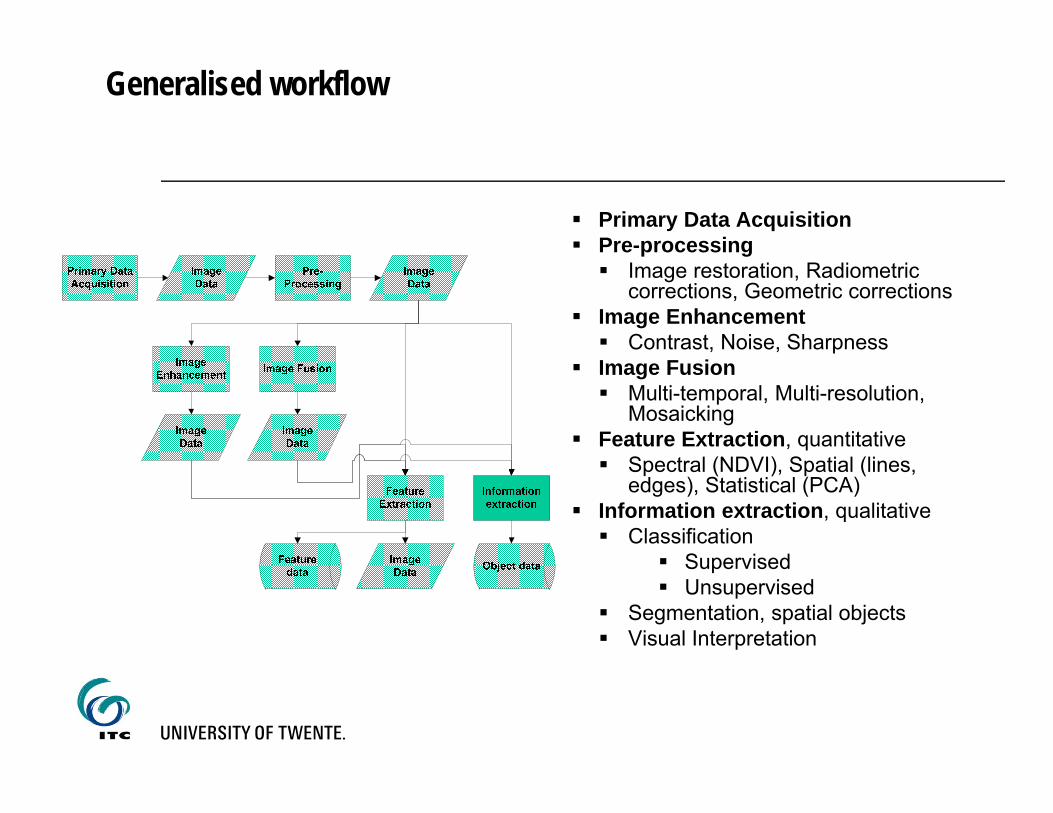
Generalised workflow
Primary Data Acquisition Pre-processing Image restoration, Radiometric
corrections, Geometric corrections Image Enhancement Contrast, Noise, Sharpness
Image Fusion Multi-temporal, Multi-resolution,
Mosaicking Feature Extraction, quantitative Spectral (NDVI), Spatial (lines,
edges), Statistical (PCA) Information extraction, qualitative Classification
Supervised Unsupervised
Segmentation, spatial objects Visual Interpretation
What are the advantages of using image classification?
We are not interested in brightness values, but in thematic characteristics
To translate continuous variability of image data into map patterns that provide meaning to the user
To obtain insight in the data with respect to ground cover and surface characteristics
To find anomalous patterns in the image data set
MULTISPECTRAL CLASSIFICATION

Why use it? - cont’ Cost efficient in the analyses of large data sets Results can be reproduced More objective then visual interpretation Effective analysis of complex multi-band (spectral)
interrelationships Classification achieves data size reduction
MULTISPECTRAL CLASSIFICATION
Together with manual digitising and photogrammetricprocessing (for map making), classification is the mostcommonly used image processing technique

Objective: Converting imagedata into thematic data
SUPERVISED CLASSIFICATION

Multi-band Image
IMAGE SPACE

One-dimensional feature space
Input layer (single)
Distinction between slices/classes
Histogram
Segmented image
unsupervised classification
No distinction between slices/classes
Histogram ?

MULTI-DIMENSIONAL FEATURE SPACE
statistical pattern recognition
feature vectors e.g.(34, 25, 117)(34, 24, 119)
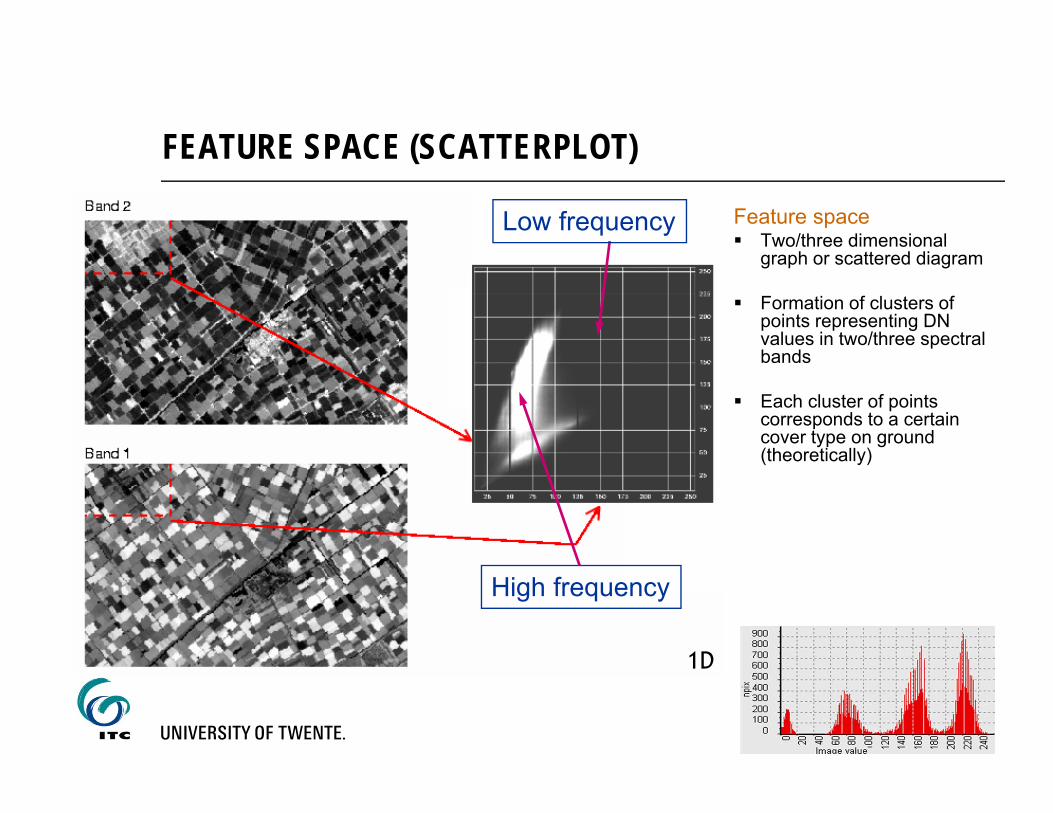
FEATURE SPACE (SCATTERPLOT)
Feature space Two/three dimensional
graph or scattered diagram
Formation of clusters of points representing DN values in two/three spectral bands
Each cluster of points corresponds to a certain cover type on ground (theoretically)
High frequency
Low frequency
1D

DISTANCES AND CLUSTERS IN FEATURE SPACE
(0,0) band x (units of 5 DN)
band y (units of 5 DN)
. .
Euclidian distance
Min y
Max y
..(0,0) Min x Max x
. .... ..
Cluster

Supervised classification procedure
1. Prepare Define/describe the classes,
define image criteria Aquire required image data
2. Define clusters in the feature space Collect ground truth Create a sample set
3. Choose a classifier / decisionrule / algorithm
4. Classify5. Validate the result
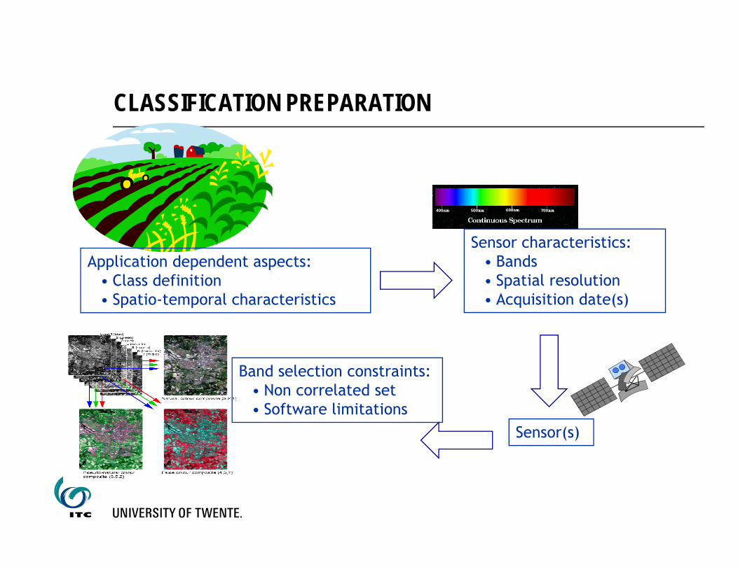
Application dependent aspects:• Class definition• Spatio-temporal characteristics
Sensor characteristics:• Bands• Spatial resolution• Acquisition date(s)
Sensor(s)
Band selection constraints:• Non correlated set• Software limitations
CLASSIFICATION PREPARATION

UNSUPERVISED APPROACH Considers only spectral distance measures Minimum user interaction Requires interpretation after classification Based on spectral groupings
SUPERVISED APPROACH Incorporates prior knowledge Requires a training set (samples) Based on spectral groupings More extensive user interaction
SUPERVISED VS. UNSUPERVISED CLASSIFICATION

UNSUPERVISED SLICING
Input layer (single)
Distinction between slices
Histogram
Segmented image
unsupervised classification
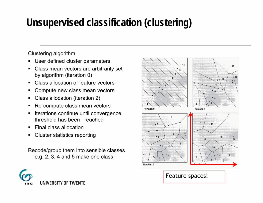
Unsupervised classification (clustering)
Clustering algorithm User defined cluster parameters Class mean vectors are arbitrarily set
by algorithm (iteration 0) Class allocation of feature vectors Compute new class mean vectors Class allocation (iteration 2) Re-compute class mean vectors Iterations continue until convergence
threshold has been reached Final class allocation Cluster statistics reporting
Recode/group them into sensible classese.g. 2, 3, 4 and 5 make one class
Feature spaces!

Supervised Classification
Principle Collect samples for training
the classifier Define clusters (decision
boundaries) in the feature space
Assign a class label to a pixel based on its feature vector and the predefined clusters in the feature space
(160,170)(160,170) = Grass
(60,40)(60,40)= House
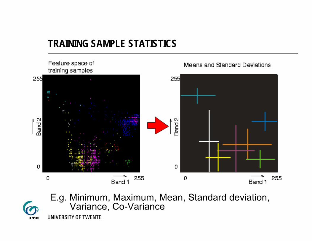
TRAINING SAMPLE STATISTICS
E.g. Minimum, Maximum, Mean, Standard deviation, Variance, Co-Variance

The points a,b and c are cluster centres of clusters A, B and C. Line ab is the distance between the cluster centres A and B.
There is overlap between the clusters A and B.
TRAINING SAMPLES IN POTENTIAL FEATURE SPACES

SAMPLE SET - 1 BAND
0 31 63 95 127 159 191 223 255
Freq.
300
200
100
0
Ground-truth
Class-Slices
Histogram of training/sample set
Samples setof classes
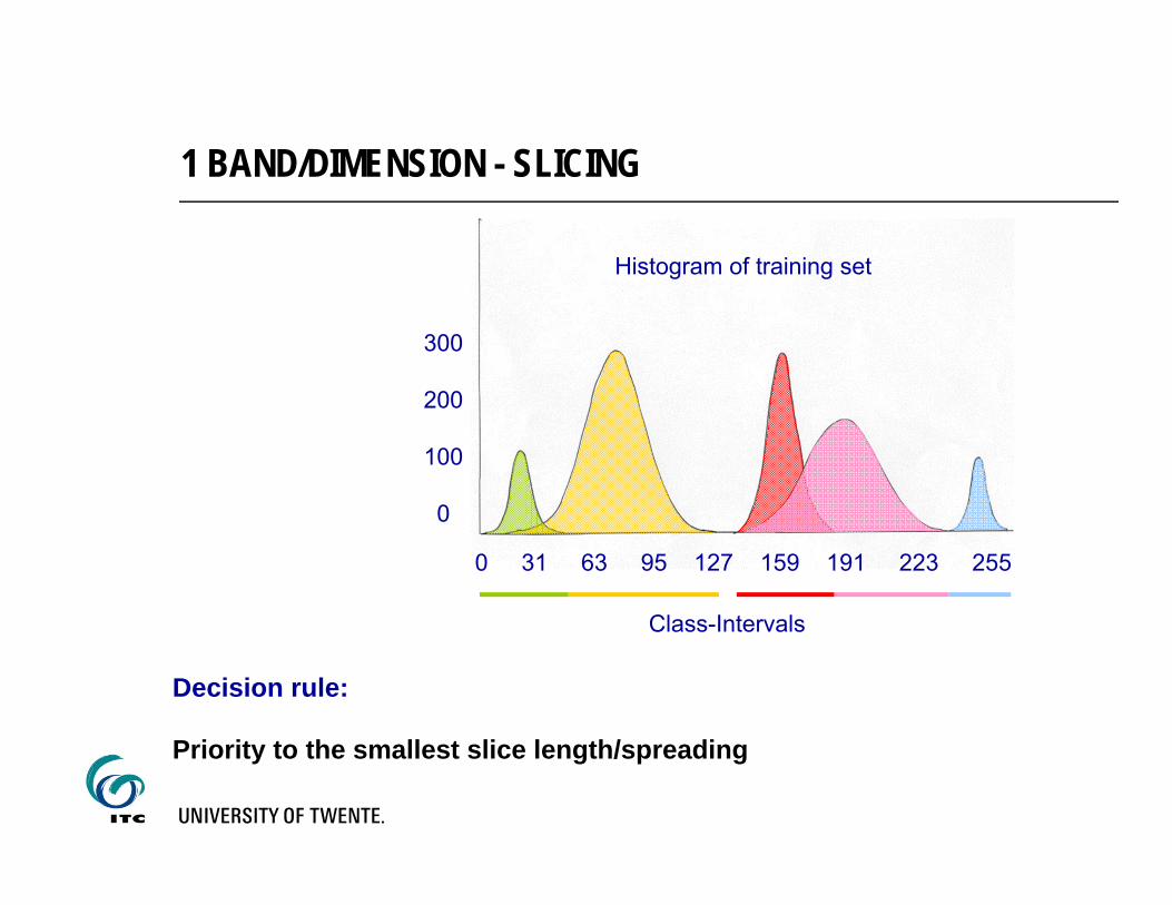
1 BAND/DIMENSION - SLICING
0 31 63 95 127 159 191 223 255
300
200
100
0
Class-Intervals
Histogram of training set
Decision rule:
Priority to the smallest slice length/spreading
0 255
0
255
Band 1
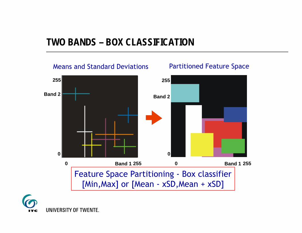
Means and Standard Deviations
0 255
0
255
Band 2
Band 1
Feature Space Partitioning - Box classifier[Min,Max] or [Mean - xSD,Mean + xSD]
Partitioned Feature Space
Band 2
TWO BANDS – BOX CLASSIFICATION

Box classification
Characteristics considers only the lower
and the upper limits of cluster
computation is simple and fast
Disadvantage overlapping boxes poorly adapted to
cluster shape
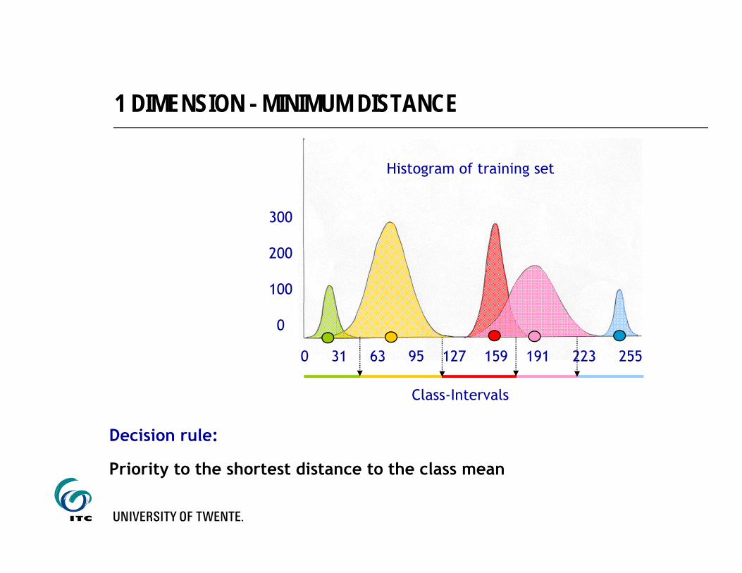
1 DIMENSION - MINIMUM DISTANCE
0 31 63 95 127 159 191 223 255
300
200
100
0
Class-Intervals
Histogram of training set
Decision rule:
Priority to the shortest distance to the class mean

Feature Space Partitioning - Minimum Distance to Mean Classifier
0
255
0 255
Band 2
Band 1
0255
Band 2
Band 1
Mean vectors
0
255
"Unknown"
2550
255
Band 2
Band 10
Threshold Distance
N DIMENSIONS – MIN. DISTANCE TO MEAN

Minimum distance to mean classifier
Characteristics emphasis on the location of
cluster centre class labelling by
considering minimum distance to the cluster centres
Disadvantage disregards the presence of
variability within a class shape and size of the
clusters are not considered

0 31 63 95 127 159 191 223 255
300
200
100
0
1 BAND – MAXIMUM LIKELIHOOD
Class-Intervals
Histogram of training set &Probability density functions
Priority to the highest probability (based upon σ and μ)
2
2
2σμ)(x
e2πσ
1f(x)
The probability that a pixel value x belongs to a class is calculated assuming a normal/Gaussian distribution
Decision rule:

255
0255
Band 2
Band 10
02550
255
Band 2
Band 1
Feature Space Partitioning -Maximum Likelihood Classifier
0 255
Band 2
Band 10
255
"Unknown"Mean vectors and variance-covariance matrices
MAXIMUM LIKELIHOOD CLASSIFIER
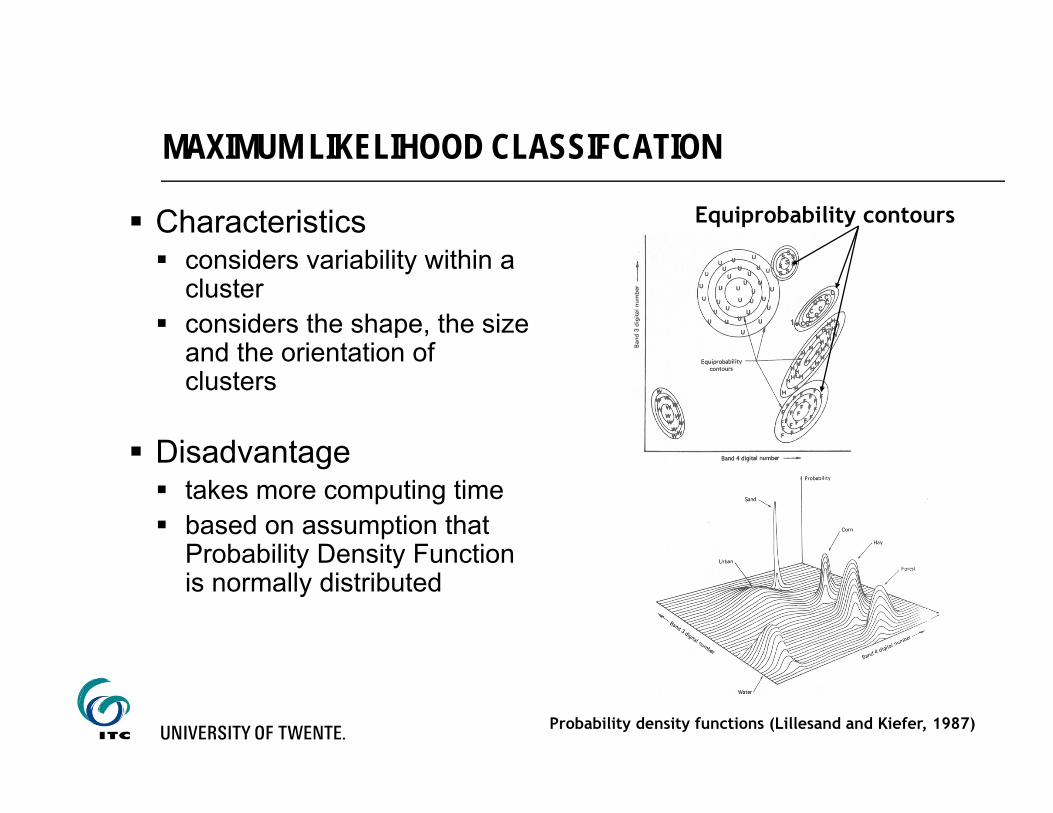
MAXIMUM LIKELIHOOD CLASSIFCATION
Characteristics considers variability within a
cluster considers the shape, the size
and the orientation of clusters
Disadvantage takes more computing time based on assumption that
Probability Density Function is normally distributed
Equiprobability contours
Probability density functions (Lillesand and Kiefer, 1987)

Systematic Sampling (n=9) Simple Random Sampling (n=9) Stratified Random Sampling (n=9)
C
A B
C
A B
C
A B
VALIDATION – SAMPLING SCHEME
Number of samples is related to: The number of samples that must be taken in order to reject a data
set as being inaccurate The number of samples required to determine the true accuracy,
within some error bounds
Sampling design:
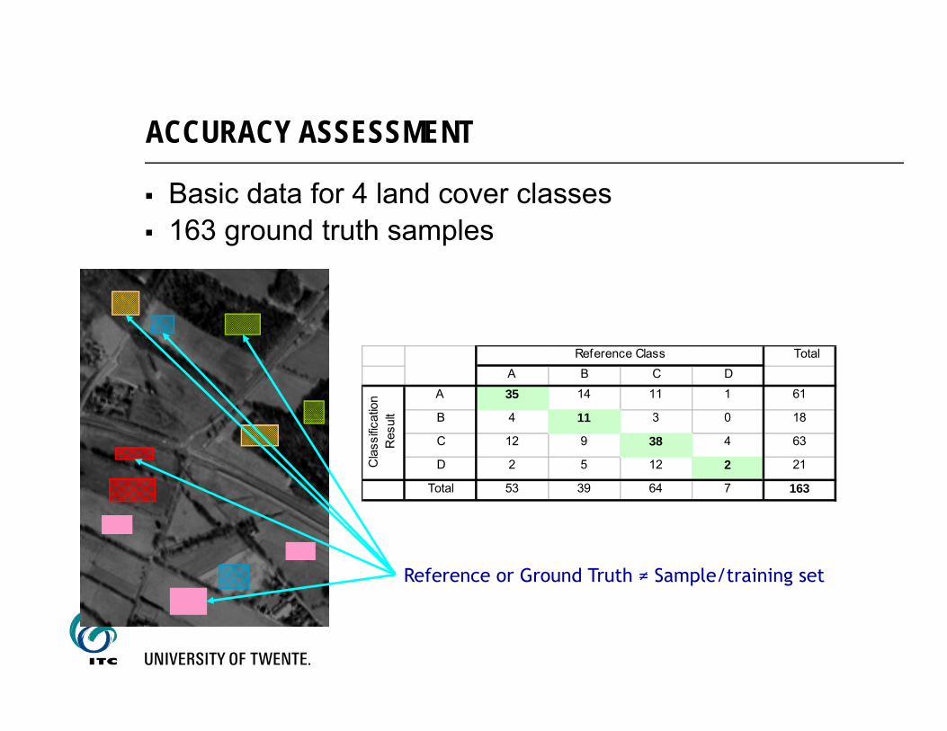
TotalA B C D
A 35 14 11 1 61
B 4 11 3 0 18
C 12 9 38 4 63
D 2 5 12 2 21
Total 53 39 64 7 163
Reference ClassC
lass
ificat
ion
Res
ult
ACCURACY ASSESSMENT
Basic data for 4 land cover classes 163 ground truth samples
Reference or Ground Truth ≠ Sample/training set

MEASURES OF THEMATIC ACCURACY
Error of commission and user accuracy Error of omission and producer accuracy
Error or confusion matrix
Total
A B C D
A 35 14 11 1 61 43% 57%
B 4 11 3 0 18 39% 61%
C 12 9 38 4 63 40% 60%
D 2 5 12 2 21 90% 10%
Total 53 39 64 7 163
34% 72% 41% 71% Overall Accuracy = SumDiag/SumTotal(4+12+2)/53 . . . . . . . . . 53%
66% 28% 59% 29%35/53 . . . . . . . . .
Producer Accuracy
Cla
ssifi
catio
nre
sult
Error ofCommision
UserAccuracy
Error of Omission
Reference Class
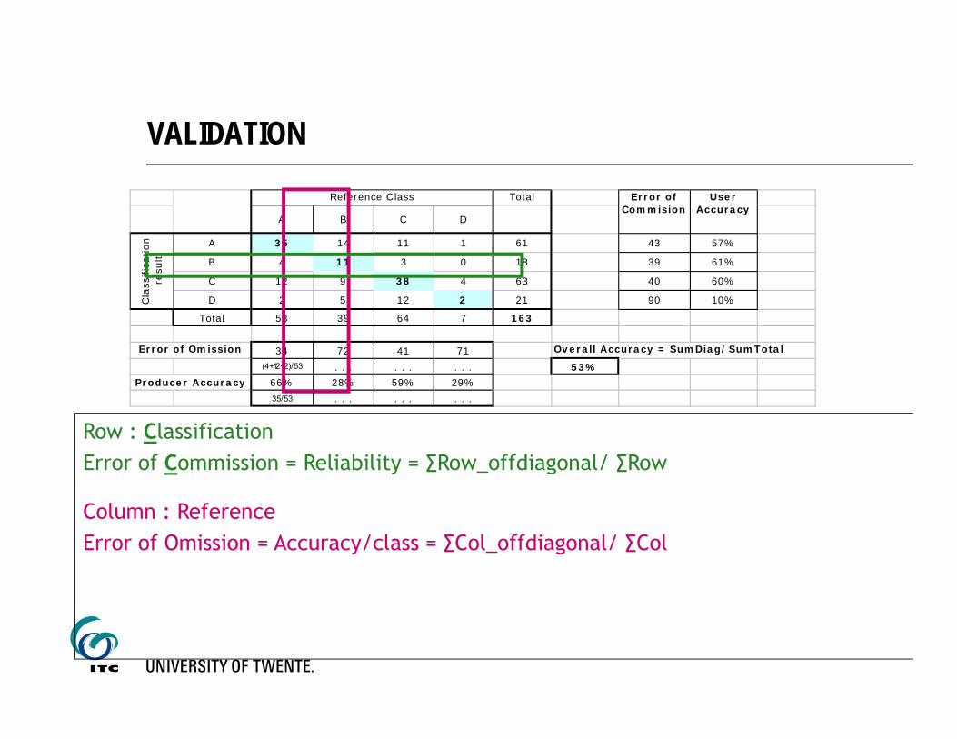
VALIDATION
Total
A B C D
A 35 14 11 1 61 43 57%
B 4 11 3 0 18 39 61%
C 12 9 38 4 63 40 60%
D 2 5 12 2 21 90 10%
Total 53 39 64 7 163
34 72 41 71 Overall Accuracy = SumDiag/SumTotal(4+12+2)/53 . . . . . . . . . 53%
66% 28% 59% 29%35/53 . . . . . . . . .
Producer Accuracy
Cla
ssifi
catio
nre
sult
Error ofCommision
UserAccuracy
Error of Omission
Reference Class
Row : ClassificationError of Commission = Reliability = ∑Row_offdiagonal/ ∑Row
Column : ReferenceError of Omission = Accuracy/class = ∑Col_offdiagonal/ ∑Col

User accuracy: Probability that a certain reference class has also been labelled as that
class. In other words, it tells us the likelihood that a pixel classified as a certain class actually represents that class (57% of what has been classified as A is A).
Producer accuracy: Probability that a reference pixel on a map is that particular class. It
indicates how well the reference pixels for that class have been classified (66% of the reference pixels A were classified as A)
Kappa statistic: Takes into account that even assigning labels at random has a certain
degree of accuracy. Kappa allows to detect if 2 datasets have a statistically different accuracy.
VALIDATION – TERMINOLOGY
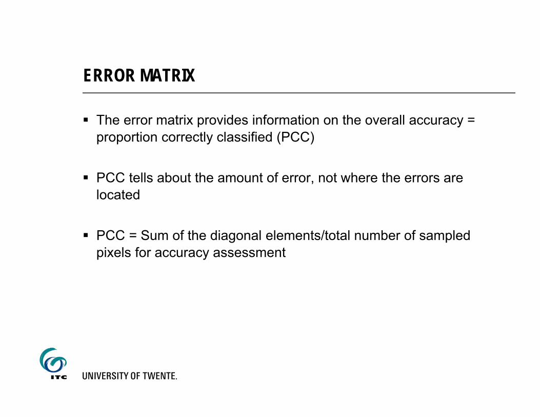
The error matrix provides information on the overall accuracy = proportion correctly classified (PCC)
PCC tells about the amount of error, not where the errors are located
PCC = Sum of the diagonal elements/total number of sampled pixels for accuracy assessment
ERROR MATRIX

Create more than 1 feature class for one land cover/use class Filter salt/pepper (majority on result) Use masks to identify areas where other rules apply (hybrid) Use multi temporal expertise to identify classes (expert
knowledge) Use other additional data (expert knowledge)
IMPROVEMENTS
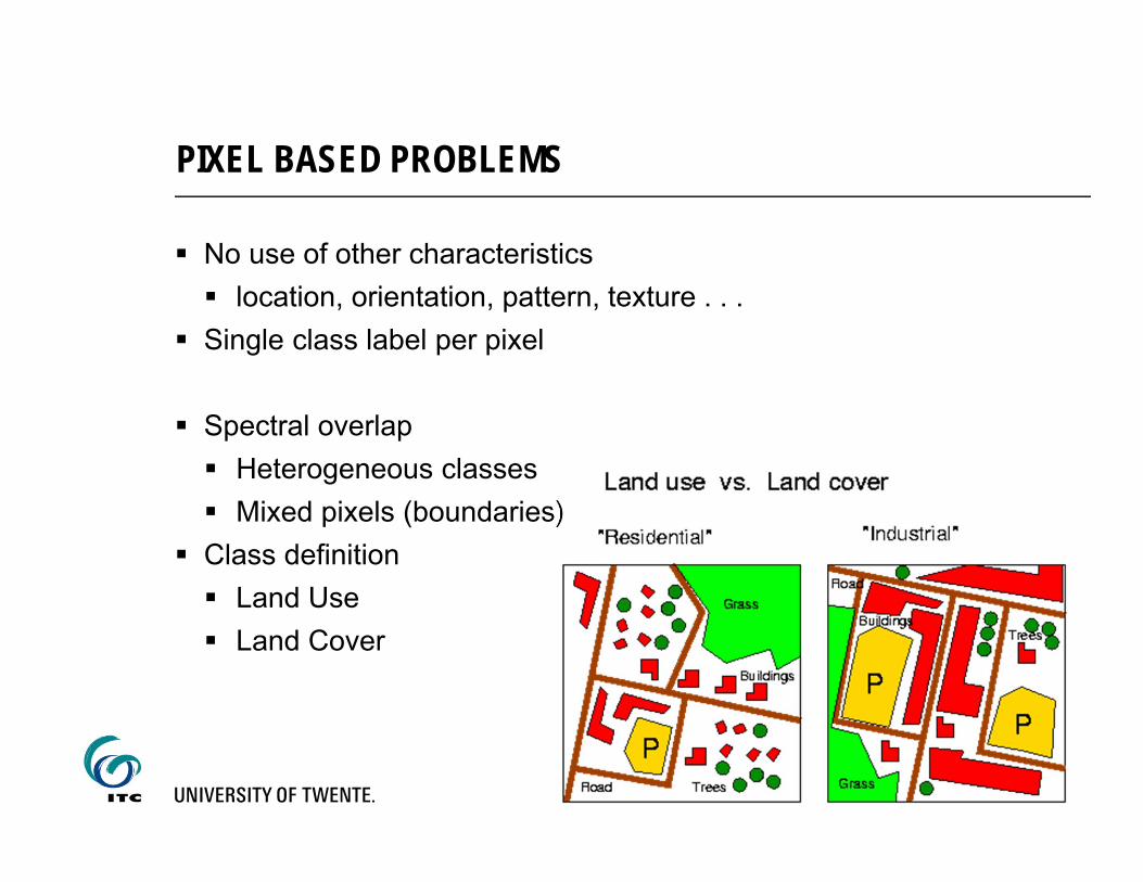
No use of other characteristics location, orientation, pattern, texture . . .
Single class label per pixel
Spectral overlap Heterogeneous classes Mixed pixels (boundaries)
Class definition Land Use Land Cover
PIXEL BASED PROBLEMS

Constraints of pixel based image classification it results in spectral classes each pixel is assigned to one class only
Spectral bands - Spectral classes - Land cover - Land use
Land cover
Grass
Training samplesSpectral classes
Meadow
Land use
Sport
PROBLEMS – LAND COVER/LAND USE

DEM or other additional datacan help improve a classification
Spectral Class Land Cover Class Land Use Classwater water shrimp cultivationgrass1grass2grass3bare soil
grassgrassgrassbare soil
nature reservenature reservenature reservenature reserve
trees1trees2trees3
forestforestforest
nature reserveproduction forestcity park
1-n and n-1 relationships can existbetween land cover and land use classes
PROBLEMS – LAND COVER/LAND USE

Objects smaller than a pixel Mixtures
Boundaries between objects Transitions
PROBLEMS – MIXED PIXELS

PROBLEMS – SPATIAL RESOLUTIONResolution dependency
Large cluster in the feature space
Spectral overlap with other classes
Distinct reflection measurement
Each pixel contains approximately the same mixture
Regular, repetition of spatial pattern

Object Based Classification
Hybrid (stratified) Classification Unsupervised/Clustering (Hyper)Spectral Classifications Subpixel Classification Expert/Knowledge Based Classification Neural Network
ALTERNATIVE PROCEDURES
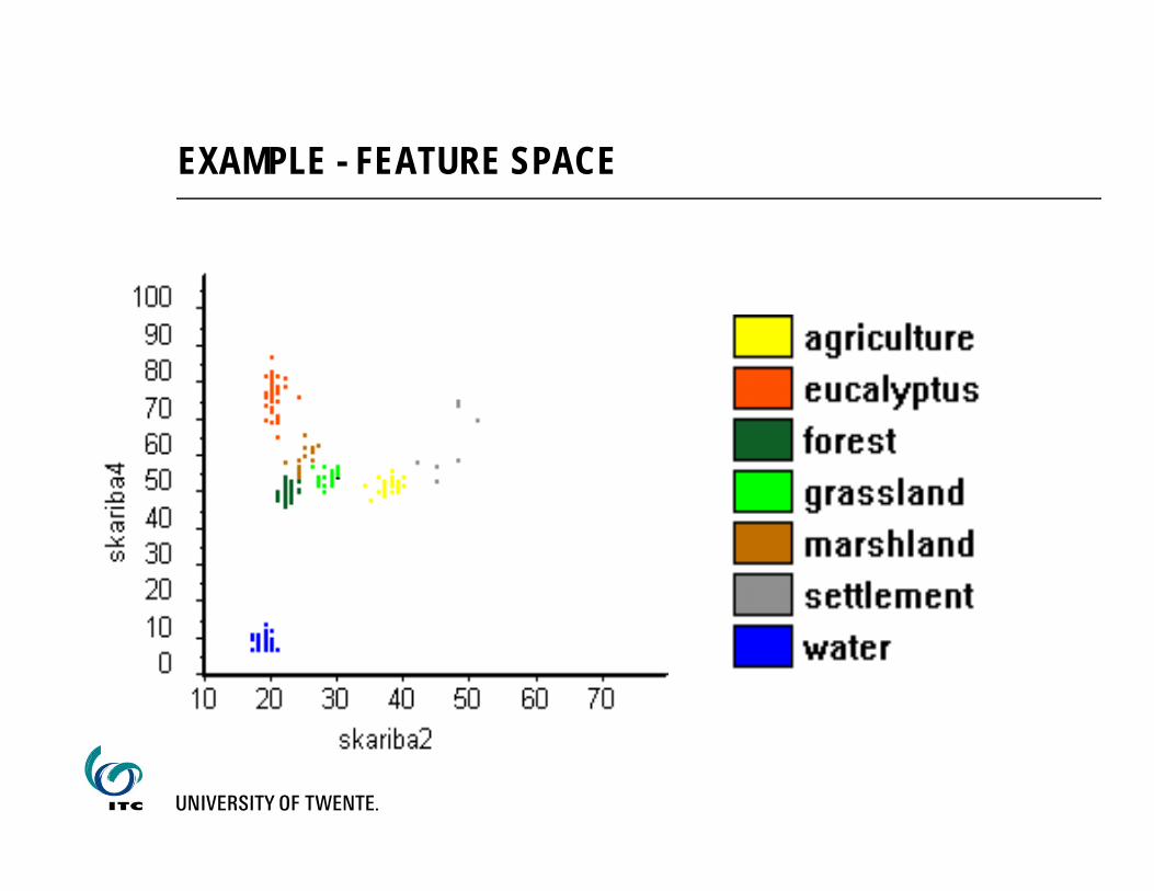
EXAMPLE - FEATURE SPACE
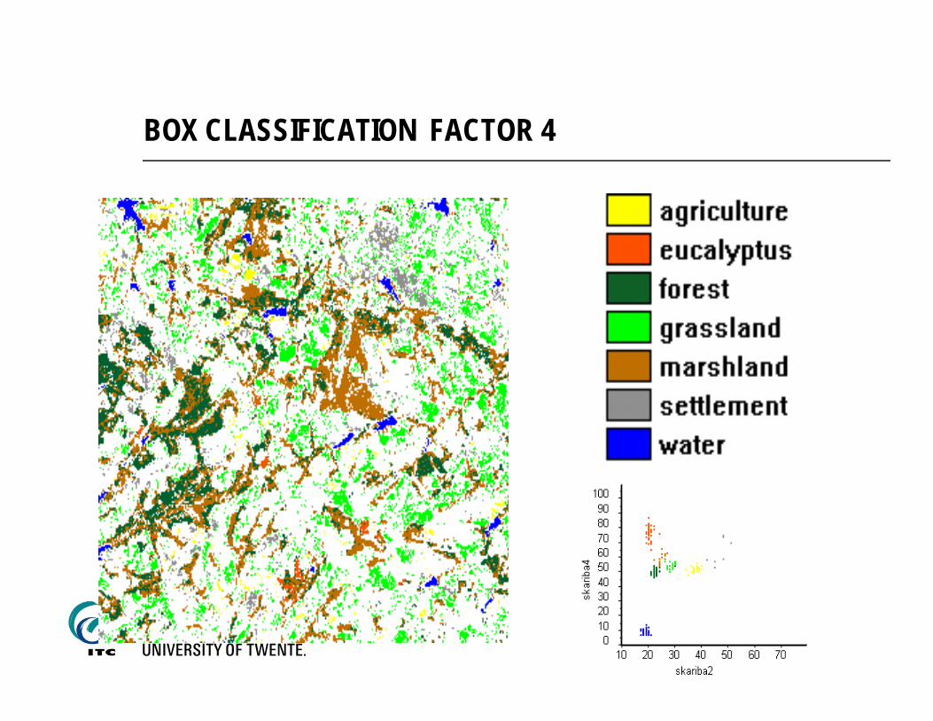
BOX CLASSIFICATION FACTOR 4
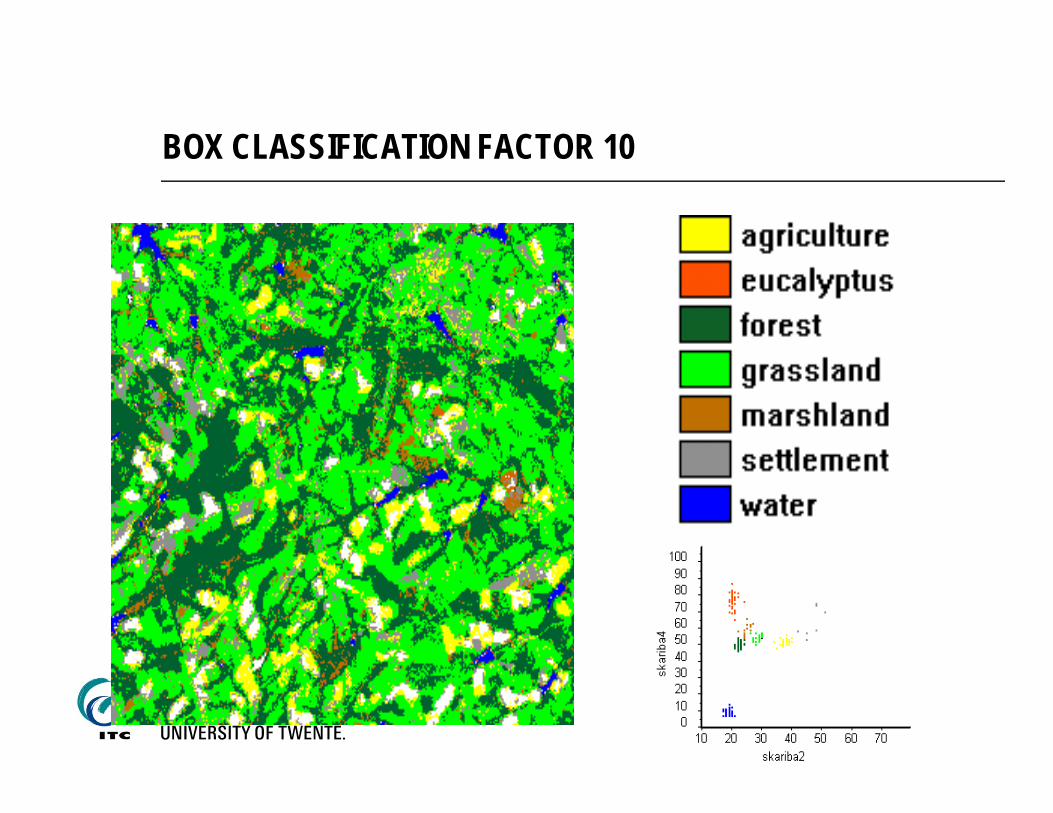
BOX CLASSIFICATION FACTOR 10
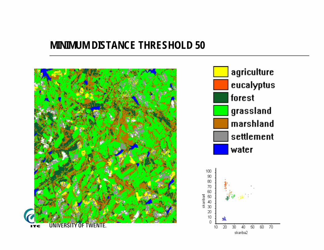
MINIMUM DISTANCE THRESHOLD 50

MINIMUM DISTANCE THRESHOLD 100

MAXIMUM LIKELIHOOD THRESHOLD 100
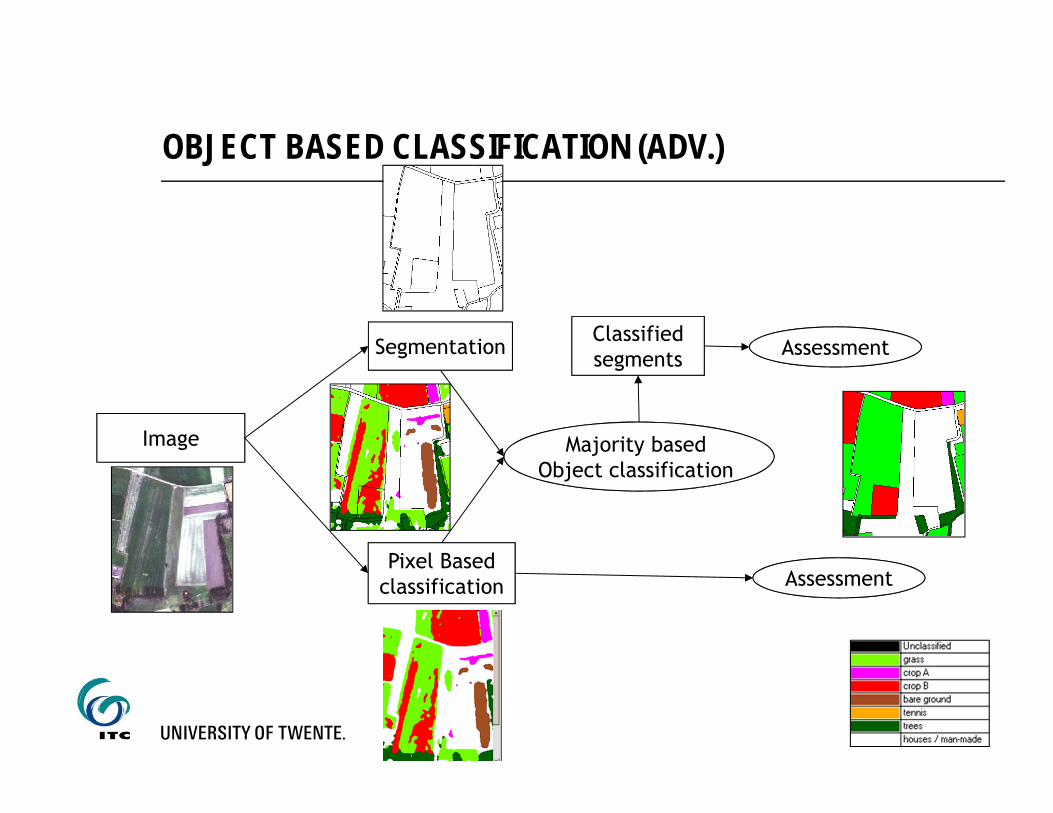
Image
Pixel Basedclassification
Segmentation
Object classification Majority based
Object classification
Classifiedsegments Assessment
Assessment
OBJECT BASED CLASSIFICATION (ADV.)
IHE: Introduction to Remote Sensing with applications in water resources
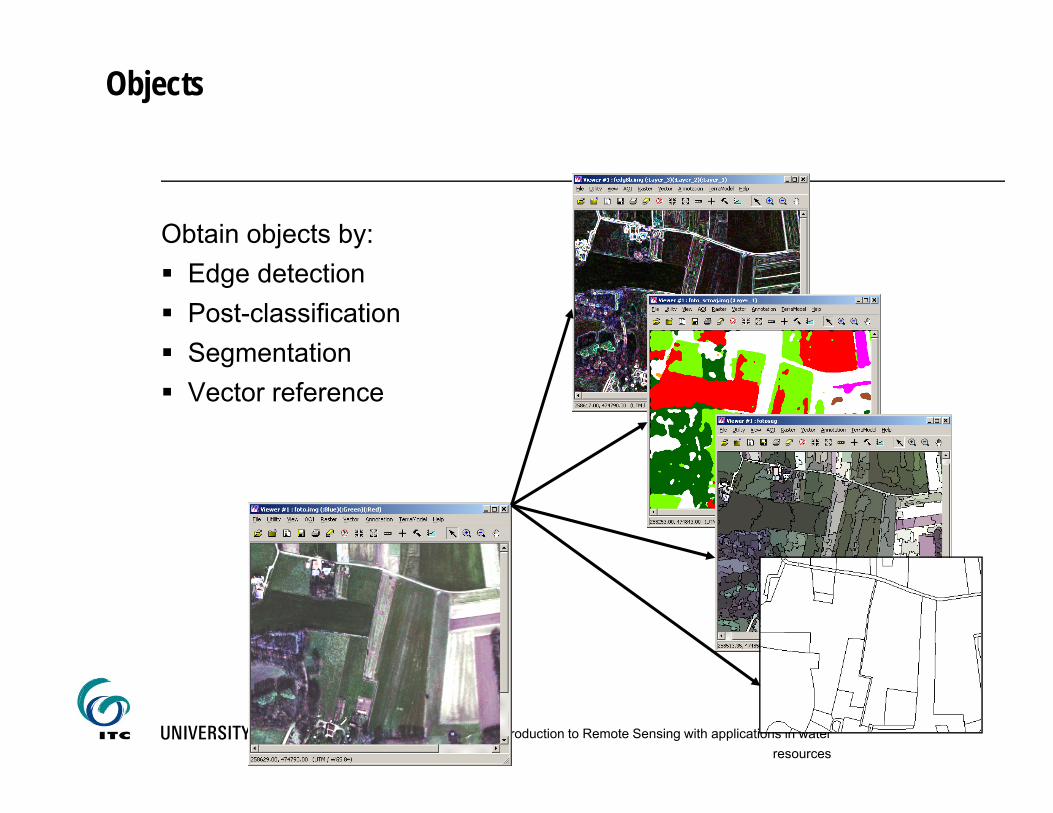
Objects
Obtain objects by: Edge detection Post-classification Segmentation Vector reference

CLASSES
Obtain class label from: Frequency/majority Object mean . . .
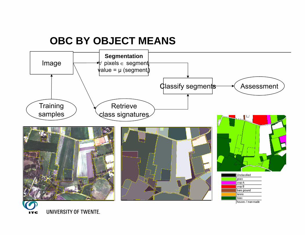
OBC BY OBJECT MEANS
Image tiv )
Segmentation pixels segmentivalue = μ (segmenti)
class signatures Retrieve
class signatures
Assessment
Trainingsamples
Classify segmentsClassify segments


