Page 1
IMAGE CLASSIFICATION USING TRANSFER LEARNING AND CONVOLUTION
NEURAL NETWORKS
A Paper
Submitted to the Graduate Faculty
of the
North Dakota State University
of Agriculture and Applied Science
By
Mohan Burugupalli
In Partial Fulfillment of the Requirements
for the Degree of
MASTER OF SCIENCE
Major Department:
Computer Science
July 2020
Fargo, North Dakota
Page 2
North Dakota State University
Graduate School
Title
IMAGE CLASSIFICATION USING TRANSFER LEARNING AND
CONVOLUTION NEURAL NETWORKS
By
Mohan Burugupalli
The Supervisory Committee certifies that this disquisition complies with North Dakota
State University’s regulations and meets the accepted standards for the degree of
MASTER OF SCIENCE
SUPERVISORY COMMITTEE:
Dr. Simone Ludwig
Chair
Dr. Saeed Salem
Dr. Maria Alfonseca Cubero
Approved:
July 30, 2020 Dr. Kendall Nygard
Date Department Chair
Page 3
iii
ABSTRACT
In the recent years, deep learning has shown to have a formidable impact on image
classification and has bolstered the advances in machine learning research. The scope of image
recognition is going to bring big changes in the Information Technology domain. This paper aims
to classify medical images by leveraging the advantages of Transfer Learning over Conventional
methods. Three types of approaches are used namely, pre-trained CNN as a Feature Extractor,
Feature Extractor with Image Augmentation, and Fine-tuning with Image Augmentation. The best
pre-trained network architectures such as VGG16, VGG19, ResNet50, Inception, Xception and
DenseNet are used for classification with each being applied to all the three approaches mentioned.
The results are captured to find the best combination of pre-trained network and an approach that
classifies the medical datasets with a higher accuracy.
Page 4
iv
ACKNOWLEDGMENTS
I would like to thank everyone who inspired me to work on the “Image Classification
project”. First and foremost, I thank my adviser, Professor Simone Ludwig for introducing me to
the concept of “Convolution Neural Networks” through her course “Advanced Intelligent
Systems”. Also, I always admire her for the quick and prompt responses, providing me all the
encouragement and support needed for completing this paperwork successfully. I would also like
to thank my committee members Professor Saeed Salem, Professor Maria Alfonseca Cubero for
their interest in my work and willingness to serve on my committee.
Finally, I would like to thank my parents and friends for their unending support and
inspiration.
Page 5
v
TABLE OF CONTENTS
ABSTRACT ................................................................................................................................... iii
ACKNOWLEDGMENTS ............................................................................................................. iv
LIST OF TABLES ....................................................................................................................... viii
LIST OF FIGURES ....................................................................................................................... ix
1. INTRODUCTION ...................................................................................................................... 1
1.1. Understanding of a Neural Network..................................................................................... 1
1.1.1. Basic Building Block of Neural Networks – “Neuron” ................................................ 1
1.1.2. Neural Network ............................................................................................................. 2
1.2. Composition of a Convolution Neural Network .................................................................. 2
1.3. Transfer Learning ................................................................................................................. 3
2. RELATED WORK ..................................................................................................................... 5
3. APPROACH ............................................................................................................................... 7
3.1. How a Computer See an Image ............................................................................................ 7
3.1.1. Colored Images .............................................................................................................. 7
3.1.2. Gray Scale Images ......................................................................................................... 8
3.2. Convolution Neural Networks.............................................................................................. 9
3.2.1. Assigning Values According to Color ........................................................................... 9
3.2.2. Selecting Features for Convolution ............................................................................. 10
3.2.3. Convolution Layer ....................................................................................................... 10
3.2.4. ReLU Layer ................................................................................................................. 12
3.2.5. Pooling Layer .............................................................................................................. 13
3.2.6. Stacking Up the Layers................................................................................................ 14
3.2.7. Fully Connected Layer ................................................................................................ 15
3.2.8. Output .......................................................................................................................... 15
Page 6
vi
3.3. Transfer Learning ............................................................................................................... 17
3.3.1. Why to Use Transfer Learning .................................................................................... 17
3.4. Architectures of Pre-trained Models .................................................................................. 20
3.4.1. VGG16 Architecture ................................................................................................... 20
3.4.2. VGG19 Architecture ................................................................................................... 21
3.4.3. ResNet50 Architecture ................................................................................................ 21
3.5. Leveraging Transfer Learning with Pre-trained CNN Models........................................... 22
3.5.1. Feature Extractor ......................................................................................................... 22
3.5.2. Feature Extractor with Image Augmentation .............................................................. 22
3.5.3. Fine-Tuning with Image Augmentation ....................................................................... 22
4. EXPERIMENTS AND RESULTS ........................................................................................... 24
4.1. Data Composition ............................................................................................................... 24
4.1.1. Initial Datasets ............................................................................................................. 24
4.1.2. Labelled and Organized Datasets ................................................................................ 24
4.2. Performance Metrics Setup ................................................................................................ 26
4.2.1. Accuracy and Precision ............................................................................................... 26
4.2.2. Recall/Sensitivity and Specificity/Selectivity ............................................................. 27
4.2.3. F1-Score ...................................................................................................................... 27
4.2.4. Confusion Matrix......................................................................................................... 28
4.2.5. ROC Curve .................................................................................................................. 28
4.3. Three Methodologies of Classification .............................................................................. 29
4.3.1. Pre-trained CNN Model as Feature Extractor ............................................................. 29
4.3.2. Pre-trained CNN Model as a Feature Extractor with Image Augmentation ................ 30
4.3.3. Pre-trained Model with Fine-Tuning and Image Augmentation ................................. 31
Page 7
vii
4.4. Evaluation Results .............................................................................................................. 33
4.4.1. Random Test Images Classification ............................................................................ 33
4.4.2. Accuracy ...................................................................................................................... 34
4.4.3. Precision ...................................................................................................................... 35
4.4.4. Recall/Sensitivity ......................................................................................................... 36
4.4.5. Specificity .................................................................................................................... 37
4.4.6. F1-score ....................................................................................................................... 38
4.4.7. Confusion Matrix to Show True Normal and True Pneumonia .................................. 39
4.4.8. ROC Curve for Best and Worst Model ....................................................................... 40
5. CONCLUSION ......................................................................................................................... 41
REFERENCES ............................................................................................................................. 42
Page 8
viii
LIST OF TABLES
Table Page
1: Demonstration of Layers in Convolution Neural Network ...................................................... 19
2: Initial Datasets .......................................................................................................................... 24
3: Labelled and Organized Datasets ............................................................................................. 25
4: True Positive, True Negative, False Positive, False Negative .................................................. 26
5: Accuracy Results ...................................................................................................................... 34
6: Precision Results ....................................................................................................................... 35
7: Recall/Sensitivity Results ......................................................................................................... 36
8: Specificity Results .................................................................................................................... 37
9: F1-Score Results ....................................................................................................................... 38
Page 9
ix
LIST OF FIGURES
Figure Page
1: Basic Neuron [2] ......................................................................................................................... 1
2: Simple Neural Network [2]......................................................................................................... 2
3: Convolution Neural Network Layers [2] .................................................................................... 3
4: Difference between Initial Layers and Later Layers [4] ............................................................. 4
5: Color Pixel Visualization [16] .................................................................................................... 7
6: Color Code Composition [1]....................................................................................................... 8
7: Gray Scale Representation of Images [19] ................................................................................. 8
8: Deformed Images of ‘X’ and ‘O’ [19] ....................................................................................... 9
9: Assigned Values for ‘X’ [19]...................................................................................................... 9
10: Selecting Features for Convolution [19] ................................................................................. 10
11: Convolution Step 1 [19] .......................................................................................................... 11
12: Convolution Step 2 [19] .......................................................................................................... 11
13: Convolution Step 3 [19] .......................................................................................................... 11
14: Convolution Step 4 [19] .......................................................................................................... 12
15: ReLU Function [19] ................................................................................................................ 12
16: ReLU Step [19] ....................................................................................................................... 13
17: Pooling Layer Step 1 [19] ....................................................................................................... 13
18: Pooling Layer Step 2 [19] ....................................................................................................... 14
19: Stacking Up of Layers Step1 [19] ........................................................................................... 14
20: Stacking Up of Layers Step 2 [19] .......................................................................................... 15
21: Fully Connected Layer [19] .................................................................................................... 15
22: Output Step 1 [19] ................................................................................................................... 16
23: Output Step 2 [19] ................................................................................................................... 16
Page 10
x
24: A Sample Image ...................................................................................................................... 18
25: Deep Neural Network [21] ..................................................................................................... 19
26: Complete Picture of CNN [41] ............................................................................................... 19
27: VGG16 Architecture [43] ....................................................................................................... 20
28: VGG19 Architecture [42] ....................................................................................................... 21
29: ResNet50 Architecture [42] .................................................................................................... 21
30: Block Diagram Showing Transfer Learning Strategies on VGG16 Model [43] .................... 23
31: Datasets ................................................................................................................................... 25
32: Accuracy vs. Precision [44] .................................................................................................... 26
33: Accuracy, Precision, Recall, Specificity, F1-Score Formulae [34] ........................................ 27
34: Confusion Matrix Demonstration [45] ................................................................................... 28
35: ROC Curve Example [40]....................................................................................................... 29
36: Illustration of Frozen Layers................................................................................................... 30
37: Illustration of Unfrozen Layers for Fine-tuning ..................................................................... 32
38: Classified Images .................................................................................................................... 33
39: Bar plot of Accuracy Values Obtained ................................................................................... 34
40: Bar Plot of Precision ............................................................................................................... 35
41: Bar Plot of Sensitivity ............................................................................................................. 36
42: Bar Plot of Specificity............................................................................................................. 37
43: Bar Plot of F1-Score ............................................................................................................... 38
44: Confusion Matrices of All Models ......................................................................................... 39
45: ROC Curve ............................................................................................................................. 40
Page 11
1
1. INTRODUCTION
Image classification has become of increasing importance recently. With the rapid growth
in Artificial Intelligence and Deep Learning, the necessity of computer vision is one of the top
priorities. The future of Image recognition and analysis is gaining momentum and is surely going
to change the world in the days to come.
1.1. Understanding of a Neural Network
Neural Networks is one of the most popular machine learning algorithms at present. It
outpaces many other peer algorithms in solving complex problems with speed and accuracy.
1.1.1. Basic Building Block of Neural Networks – “Neuron”
From the biological definition, a neuron is the basic working unit of the brain that takes
sensory input from the external world and transmits the response to other nerve cells, muscle or
gland cells to perform the respective action [2]. In simple terms, it receives an input signal, process
it and delivers an output signal.
Similarly, a neuron in machine learning is defined as a placeholder for a mathematical
function, that takes input and performs the given function on them to provide an output [2][3]. The
function used in neuron is generally termed as activation function.
Figure 1 describes X1, X2, X3 as inputs fed to a neuron. It delivers a result output after
applying the function on the inputs given.
Figure 1: Basic Neuron [2]
Page 12
2
1.1.2. Neural Network
The fundamental blocks in Neural networks are called layers. A layer is a collection of
neurons that takes an input and provide an output. Each neuron has its own function and the inputs
are processed layer by layer [2].
Figure 2 describes the leftmost layer as the input layer, rightmost layer is the output layer
and the middle layer is called hidden layer. The number and type of hidden layers differ according
to the problem. If the neural network has more than 3 or 4 hidden layers, it is called as Deep Neural
Network.
Figure 2: Simple Neural Network [2]
1.2. Composition of a Convolution Neural Network
The general activation functions used in most neural networks are step, sigmoid, tanh,
ReLU and leaky ReLU. Instead of these activation functions, if we use convolution and pooling
functions as activation functions in the hidden layers of the neural network, then it is called as
Convolution Neural Network.
Page 13
3
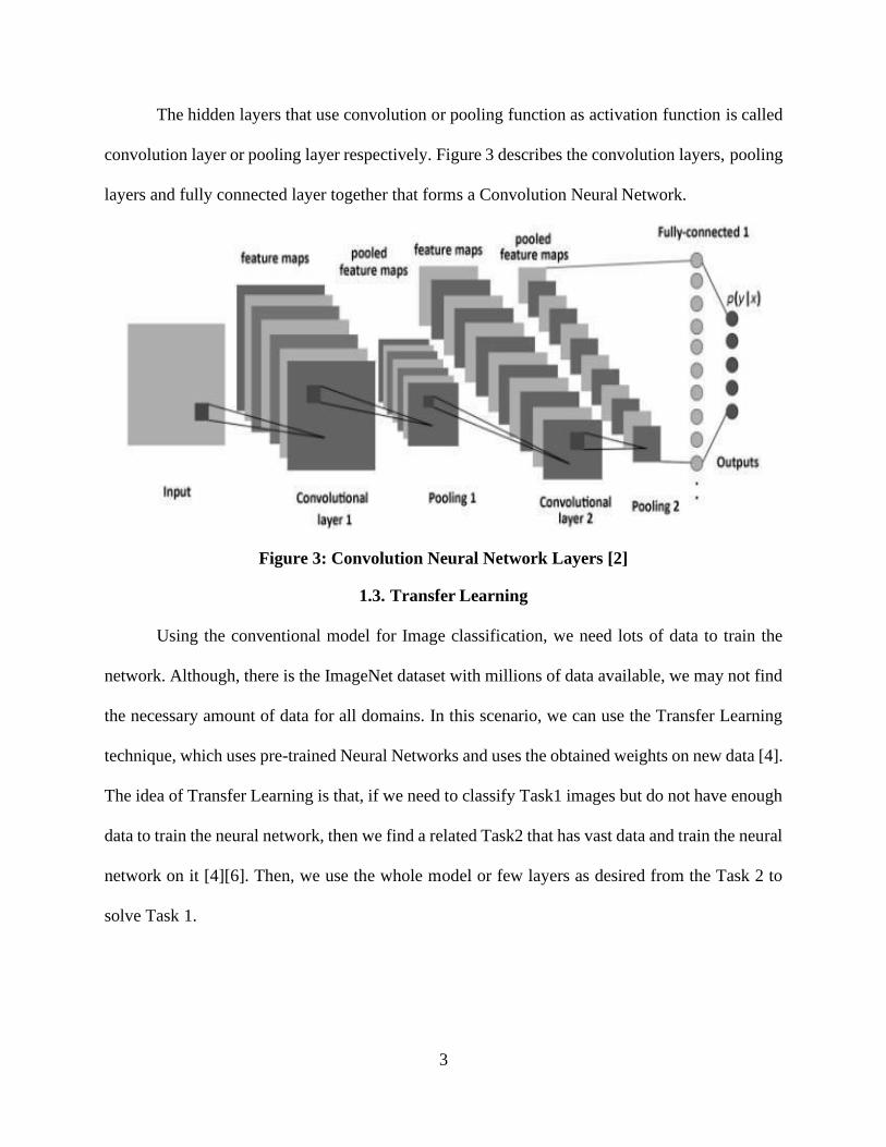
The hidden layers that use convolution or pooling function as activation function is called
convolution layer or pooling layer respectively. Figure 3 describes the convolution layers, pooling
layers and fully connected layer together that forms a Convolution Neural Network.
Figure 3: Convolution Neural Network Layers [2]
1.3. Transfer Learning
Using the conventional model for Image classification, we need lots of data to train the
network. Although, there is the ImageNet dataset with millions of data available, we may not find
the necessary amount of data for all domains. In this scenario, we can use the Transfer Learning
technique, which uses pre-trained Neural Networks and uses the obtained weights on new data [4].
The idea of Transfer Learning is that, if we need to classify Task1 images but do not have enough
data to train the neural network, then we find a related Task2 that has vast data and train the neural
network on it [4][6]. Then, we use the whole model or few layers as desired from the Task 2 to
solve Task 1.
Page 14
4
Figure 4 describes the earlier layers of ConvNet that deals with generic features such as
edge detectors, texture detectors, patterns, etc. The later layers to the end of the network become
more specific to the details of the image dataset [7]. Here come the advantages of Transfer
Learning. We will fix/freeze the earlier layers of the pre-trained network and retrain the rest of the
layers with fine tuning of backpropagation. Instead of training our network from the first layer, we
just transfer the weights already learned by a pre-trained network such as VGG16 and save time
and efforts [8][9].
Figure 4: Difference between Initial Layers and Later Layers [4]
Page 15
5
2. RELATED WORK
The growing medical usability of Image classification attracts the attention of many
researchers to do further investigation on the concepts of Convolution Neural Networks. One of
the ways of investigation is the detection of pneumonia from X-ray chest images using Transfer
Learning technique. Kermany et al. in [10] presented medical diagnoses and treatable diseases by
using image-based deep learning models to detect or classify different medical datasets. They used
the Inception V3 architecture for pre-training the model on the ImageNet dataset. Here, the
convolution layers were frozen and used as fixed feature extractors. Initially generated bottleneck
features from training on the ImageNet dataset and utilized them to train and classify X-ray images.
The testing accuracy for chest X-rays for pneumonia detection was 92.80 %.
Stephen et al. in [11] presented an efficient deep learning approach to pneumonia
classification in healthcare. The authors proposed a deep learning model with 4 convolutional
layers and 2 dense layers in addition to classical image augmentation. They did not use any pre-
trained networks rather developed a CNN from scratch to extract features from a given chest X-
ray image and classify it to determine if a person is infected with pneumonia. They used the image
augmentation concept to mitigate the reliability and interpretability challenges often faced when
dealing with medical imagery and achieved 93.73% testing accuracy.
Wu et al. in [12] presented a model to predict pneumonia with chest X-ray images based
on convolutional deep neural learning networks and random forest. Initially, the authors used
adaptive median filtering to improve the quality of images. Then, established the CNN architecture
based on Dropout to extract deep activation features from each chest X-ray image. Finally,
employed the Random Forest classifier based on GridSearchCV class as a classifier for deep
activation features in CNN model. The authors achieved 97 % testing accuracy.
Page 16
6
Liang and Zheng in [13] presented a transfer learning method with a deep residual network
for pediatric pneumonia diagnosis. The authors a deep learning model with 49 convolutional layers
and 2 dense layers and achieved 96.70% testing accuracy. Their paper has shown that deep learning
does not require feature processing of input data compared to traditional supervised pattern
recognition methods, and model performance is not limited by the medical diagnostic experience
owned by the designer, thus having an unparalleled advantage.
Lung cancer accounts for 26 % of all cancer deaths in 2017, accounting for more than 1.5
million deaths. Thus, Nobrega et al. in [14] proposed to explore the performance of deep transfer
learning to classify pulmonary nodule malignancies. In this work, they have used a convolutional
neural network such as VGG16, VGG19, MobileNet, Xception, InceptionV3, ResNet50,
Inception-ResNet-V2, DenseNet169, DenseNet201, NASNetMobile and NASNetLarge, where
they were used to extract parameters from an image database of the lung. The characteristics were
classified using Naive Bayes, Perceptron multilayer, support vector machine, Near Neighbors and
Random Forest and achieved 95.3% testing accuracy.
All the above-related works used the chest X-ray images for pneumonia classification in
different methodologies. The main difference between our proposed model and other related works
according to literature surveys; this paper considered one of the methods to use the data
augmentation to generate more images and make the proposed model immune from a smaller
number of datasets. We used feature extraction with fine-tuning that re-trains the weights in
‘unfreeze layers’ by backward propagation. Also, we showed the implementation using the top
best pre-trained networks of Transfer Learning and compared all of them in terms of accuracy,
precision, sensitivity, specificity and F1-score.
Page 17
7
3. APPROACH
3.1. How a Computer See an Image
A computer understands an image using numbers for each pixel. The smallest element of
an image is called a pixel, which is basically a dot as shown in Figure 5. If an image is said to have
resolution 250*350, it means it’s 250 pixels wide and 350 pixels high [16]. We can describe images
into two types according to their color, namely colored and gray scale (black and white).
Figure 5: Color Pixel Visualization [16]
3.1.1. Colored Images
In color images, pixels are represented in the RGB color model. RGB stands for Red Green
Blue and represents a tuple of three components. Each component can take a value between 0 and
255, where the tuple (0,0,0) represents black and (255,255,255) represents white [17]. All colors
that humans perceive are various combinations of red, green and blue. Figure 6 describes a few
more examples of color notations in RGB model. If an image is represented as 250*350*3 pixels,
the last pixel indicates the three components of the RGB tuple. We can convert a colored image
to gray scale and vice-versa by applying transformation on the tuple values respectively.
Page 18
8
Figure 6: Color Code Composition [1]
3.1.2. Gray Scale Images
In grayscale (black and white) images, each pixel is a single number representing the
amount of light, or intensity, it carries. In most of the cases, the range of intensities are used which
are from 0(black) to 255(white). Everything between 0 and 255 is various shades of gray. Figure
7 describes the clear view of a gray scale image as seen by a computer. Colored images can be
converted to gray scale and vice-versa by altering the RGB tuple components [18].
Figure 7: Gray Scale Representation of Images [19]
Page 19
9
3.2. Convolution Neural Networks
CNNs are a combination of convolution, ReLU, pooling and fully connected layers [19].
If we need to predict ‘X’ vs ‘O’ images, there can be trickier cases where images are deformed.
We need to classify all images to either ‘X’ or ‘O’ irrespective of deformations. Using normal
techniques, computers compare images for classification and the deformed images cannot be
classified. Here comes the use of CNNs that can classify normal as well as deformed.
Figure 8: Deformed Images of ‘X’ and ‘O’ [19]
3.2.1. Assigning Values According to Color
As the computer understands an image using numbers at each pixel and the intensity is
same throughout the ‘X’ or ‘O’, let’s use value 1 for black pixel and -1 for white pixel as shown
in Figure 9 [19].
Figure 9: Assigned Values for ‘X’ [19]
Page 20
10
3.2.2. Selecting Features for Convolution
CNN compares images piece by piece. The pieces that it looks for are called features. By
finding rough feature matches, in roughly the same position in two images, CNN gets a lot better
at seeing similarity than whole-image matching schemes. Figure 10 describes the three features or
filters used in this case [19].
Figure 10: Selecting Features for Convolution [19]
3.2.3. Convolution Layer
Here we will move each feature/filter to every possible position on the image. Multiply
each image pixel by the corresponding feature pixel and finish a result matrix as described in
Figure 11. The next step is to add all the elements in the result matrix and divide by total number
of pixels in the feature. To create a map put the value of a filter at that respective place as shown
in Figure 12.
Similarly, move the filter/feature to every other positions of the image and will see how
the feature matches that area. Finally, we will get an output as shown in Figure 13 for one feature.
After performing the same process for the other two filters as well, we get the convolution results
for all the features as shown in Figure 14.
Page 21
11
Figure 11: Convolution Step 1 [19]
Figure 12: Convolution Step 2 [19]
Figure 13: Convolution Step 3 [19]
Page 22
12
Figure 14: Convolution Step 4 [19]
3.2.4. ReLU Layer
Rectified Linear Unit (ReLU) is an activation function that activates a node if the input is
above a certain quantity. While the input is below zero, the output is zero, but when the output
rises above a certain threshold, it has a linear relationship with the dependent variable as shown in
Figure 15 [20].
In this layer we remove every negative value from convolution results and replace it with
zeros. This is done to avoid the values from summing up to zero. The output for one feature looks
like as shown in Figure 16. Likewise, we must calculate ReLU activation results for all features.
Figure 15: ReLU Function [19]
Page 23
13
Figure 16: ReLU Step [19]
3.2.5. Pooling Layer
In this layer, the image stack is shrunk into a smaller size. We use the max pooling function
here. The steps include picking a window size (usually 2 or 3), pick a stride (usually 2), walk the
window across the ReLU results, from each window take the maximum value. Let us see results
after performing pooling with a window size 2 and a stride 2 on first filtered image.
In the first window the maximum or highest value is 1, so we track that and move the
window two strides. Figure 17 describes the pooling of one 2*2 window.
After doing the pooling for entire image, we get the result as shown in Figure 18. We can
see that the result matrix got reduced from 7*7 to 4*4 of size. Repeat the process for all three
outputs that we got after ReLU layer and we get 4*4 matrix for each respectively.
Figure 17: Pooling Layer Step 1 [19]
Page 24
14
Figure 18: Pooling Layer Step 2 [19]
3.2.6. Stacking Up the Layers
After passing through Convolution, ReLU and Pooling we get the 4*4 matrices from the
input image [21] as shown in Figure 19.
Figure 19: Stacking Up of Layers Step1 [19]
Page 25
15
Figure 20: Stacking Up of Layers Step 2 [19]
3.2.7. Fully Connected Layer
This is the final layer where the actual classification happens. Here we take our filtered and
shrunk images and put them into a single list or a vector as shown in Figure 21.
Figure 21: Fully Connected Layer [19]
3.2.8. Output
We can see that certain values in the list are high for ‘X’ and if we repeat the entire process
for ‘O’ there will be certain different values which are high. For ‘X’ 1, 4, 5, 10, 11 vectors are high
and for ‘O’ 2, 3, 9, 12 element vectors are high. Now, as shown in Figure 22, the model is trained
with the vectors to classify between ‘X’ and ‘O’.
Page 26
16
Consider we have given a new input image for classification. That image passes through
all the layers and got the corresponding 12 element vector as shown in Figure 23. We compare
with the list of ‘X’ and ‘O’. For ‘X’ there are certain values which are high (1,4,5,10,11) and sum
these vectors which is 5. Sum the corresponding vectors of input image which is 4.96. Divide by
5 and we get 0.91. Similarly, for ‘O’ we get 0.51. As 0.91 is greater than 0.51, the input image is
classified as ‘X’.
Figure 22: Output Step 1 [19]
Figure 23: Output Step 2 [19]
Page 27
17
3.3. Transfer Learning
In context of deep learning, most models need lots of data, and obtaining a large amount
of labeled data for a variety of domains can be difficult, considering the time and effort it takes to
label the data. Although there is ImageNet dataset with millions of data, getting data for every
domain is tough. While there are state-of-the-art models which give high accuracy, they would be
only on specific datasets and when used on new similar task, they suffer a significant loss. This
forms the basis for transfer learning which used knowledge gained from pre-trained networks and
use it to solve new similar problems [22].
3.3.1. Why to Use Transfer Learning
Consider Figure 24 for training with label as an elephant. It is of size 225*150 pixels taking
color pixel as a single component. As ‘X’ and ‘O’ are simple, we just used three filters. Here, we
must take hundreds or even thousands of filters for convolution. If each filter is of size 3*3, it must
perform convolution on the given image which is 225*150 pixels. That is, each feature generates
a 75*50 size matrix. All filters together generate thousands of similar matrices which takes lot of
computational time and memory. Figure 25 shows the sample computations visual for each layer.
Apart from this, there is still ReLU and pooling functions in each block as shown in Figure 26. In
summary, if we have 3000 training images of 228*150 pixels each, the computations for the initial
block are as shown in Table 1.
The initial layers perform a lot of computations and as passed to the next block the number
of computations decreases due to the convolution and pooling in the previous blocks. To train the
model on one image, the computations of first block are as shown in Table 1. If the training images
are around 3,000, these computations are multiplied by the same amount which need huge
memory, time and computational power.
Page 28
18
Here comes the use of pre-trained networks which are already trained on millions of
ImageNet datasets and can be used instantly for classification. However, all types of images are
not available in ImageNet and the pre-trained networks become obsolete if they need to classify
new set of images which are out of scope of the ImageNet datasets.
The solution for this is to use Transfer Learning. It enables us to utilize knowledge from
previously learned tasks and apply on new similar tasks. In computer vision domain, the initial
blocks of CNN extract certain low-level features such as edges, shapes, corners, intensity etc. As
we know that initial blocks use more computational power, we transfer the knowledge (features,
weights) of them from a pre-trained network and utilize to classify new images. The last blocks in
CNN are more specific to image details and hence we freeze the top layers and use the bottom
layers as per the problem.
Figure 24: A Sample Image
Page 29
19
Figure 25: Deep Neural Network [21]
Figure 26: Complete Picture of CNN [41]
Table 1: Demonstration of Layers in Convolution Neural Network
Block 1 For One training image of 225*150 pixels
Input Output
Convolution Layer let 100 number of filters Hundred 75*50 matrices
ReLU Layer Hundred 75*50 matrices Hundred 75*50 matrices
Pooling layer Hundred 75*50 matrices Hundred 36*25 matrices
Page 30
20
3.4. Architectures of Pre-trained Models
In all pre-trained networks, we use all the convolution layers for feature extraction. We
then replace the fully connected and dense layer with our own layers to classify the images as
normal or pneumonia. With fine-tuning in place, we unfreeze last couple of blocks before fully
connected layers. These blocks adjust their weights with respect to loss function using
backpropagation technique. Let us have a look at a couple of architectures [25].
3.4.1. VGG16 Architecture
This is a 16-layer (convolution and fully connected) network built on the ImageNet
database for the purpose image classification. Figure 27 describes the architecture of the model.
From the image, we can see that there are 13 convolution layers using 3*3 filters along
with max pooling and two fully connected hidden layers of 4,096 units in each layer followed by
a dense layer of 1,000 units, where each unit represents one of the image categories in the
ImageNet database.
Figure 27: VGG16 Architecture [43]
Page 31
21
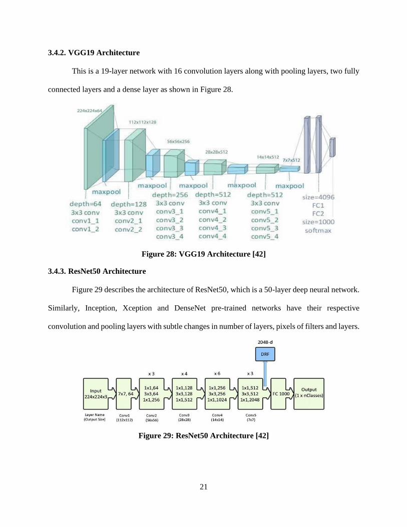
3.4.2. VGG19 Architecture
This is a 19-layer network with 16 convolution layers along with pooling layers, two fully
connected layers and a dense layer as shown in Figure 28.
Figure 28: VGG19 Architecture [42]
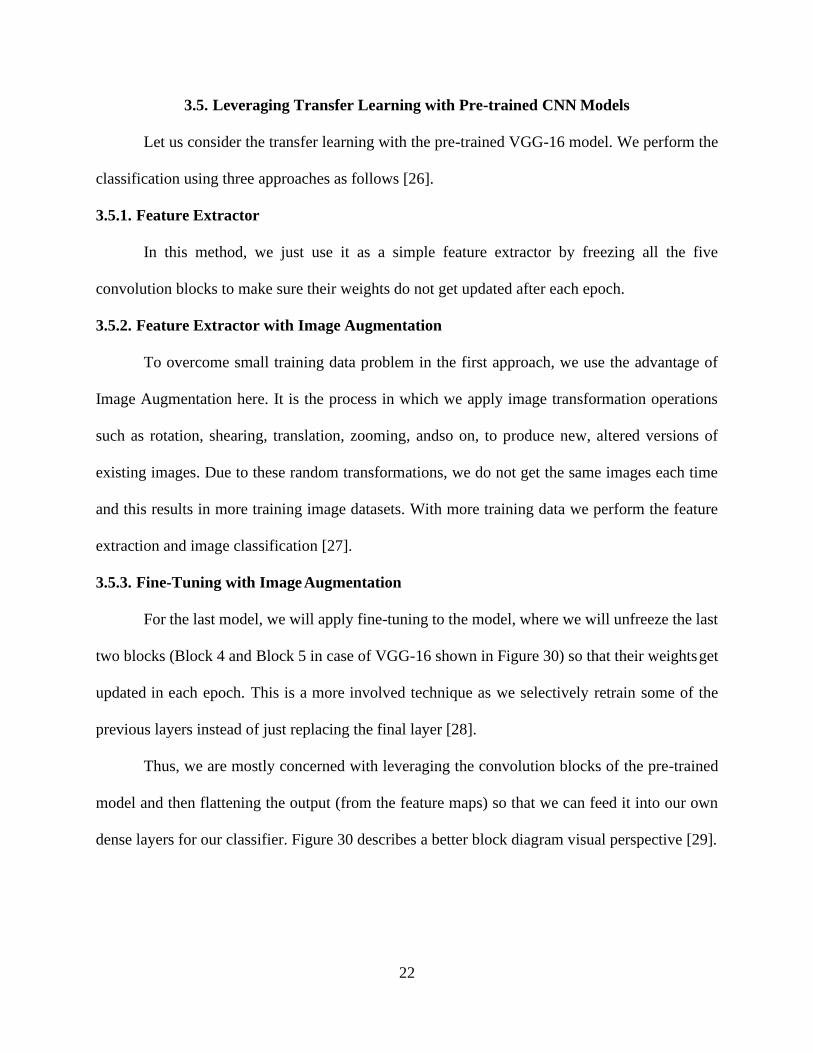
3.4.3. ResNet50 Architecture
Figure 29 describes the architecture of ResNet50, which is a 50-layer deep neural network.
Similarly, Inception, Xception and DenseNet pre-trained networks have their respective
convolution and pooling layers with subtle changes in number of layers, pixels of filters and layers.
Figure 29: ResNet50 Architecture [42]
Page 32
22
3.5. Leveraging Transfer Learning with Pre-trained CNN Models
Let us consider the transfer learning with the pre-trained VGG-16 model. We perform the
classification using three approaches as follows [26].
3.5.1. Feature Extractor
In this method, we just use it as a simple feature extractor by freezing all the five
convolution blocks to make sure their weights do not get updated after each epoch.
3.5.2. Feature Extractor with Image Augmentation
To overcome small training data problem in the first approach, we use the advantage of
Image Augmentation here. It is the process in which we apply image transformation operations
such as rotation, shearing, translation, zooming, andso on, to produce new, altered versions of
existing images. Due to these random transformations, we do not get the same images each time
and this results in more training image datasets. With more training data we perform the feature
extraction and image classification [27].
3.5.3. Fine-Tuning with Image Augmentation
For the last model, we will apply fine-tuning to the model, where we will unfreeze the last
two blocks (Block 4 and Block 5 in case of VGG-16 shown in Figure 30) so that their weights get
updated in each epoch. This is a more involved technique as we selectively retrain some of the
previous layers instead of just replacing the final layer [28].
Thus, we are mostly concerned with leveraging the convolution blocks of the pre-trained
model and then flattening the output (from the feature maps) so that we can feed it into our own
dense layers for our classifier. Figure 30 describes a better block diagram visual perspective [29].
Page 33
23
Figure 30: Block Diagram Showing Transfer Learning Strategies on VGG16 Model [43]
Page 34
24
4. EXPERIMENTS AND RESULTS
4.1. Data Composition
4.1.1. Initial Datasets
The initial raw datasets are unlabeled images with the number of images in each category
as described in Table 2.
Table 2: Initial Datasets
Number of Images
Data type NORMAL PNEUMONIA
Test 234 390
Train 1341 3875
Val 8 8
4.1.2. Labelled and Organized Datasets
In neural networks, better accuracies can be achieved with more training data. A good
number of validation data is required to calculate the accurate validation loss after each epoch and
backpropagate the error to correct the weights in the desired layers. The test data should be
maintained to check the results and performance accuracy. Neural networks need the label dataof
each image to train, validate and test them appropriately. With these points in mind, the data is
split proportionally as shown in Table 3, and the images are labelled as NORMAL and
PNEUMONIA, respectively.
Considering the VGG-16 model to demonstrate the experiments, the datafile has test, train
and validation data in the test, train and val subfolders. Each category (test/train/val) of the data
folder has NORMAL/PNEUMONIA subfolders that contain the respective images.
Create train, test and validation lists. Append images locations to these lists according to
labels. Example: x_train contains all NORMAL Images from training dataset and y_train contains
all PNEUMONIA images of training dataset. Figure 31 describes datasets count for each category.
Page 35
25
Resize and convert the images to array using the python inbuilt library ‘array_to_img’.
Store the arrays in separate lists for training and validation. Split the labels and store in labels list.
Training dataset shape and Validation dataset shape now is: (5000, 150, 150, 3) and (80, 150, 150,
3) respectively.
Scale the images and transform the labels using ‘LabelEncoder’ library. Import and Load
the chosen model with ‘imagenet’ as weights.
Table 3: Labelled and Organized Datasets
Number of Images
Data type NORMAL PNEUMONIA Total
Test 300 390 690
Train 1200 3800 5000
Val 80 80 160
Figure 31: Datasets
Page 36
26
4.2. Performance Metrics Setup
The labels of all test data are available for the classification. The new predicted labels are
then compared with the existing labels [33]. From the comparison we find the measures as
described in Table 4.
• True positive: Pneumonia images correctly identified as pneumonia
• False positive: Normal images incorrectly identified as pneumonia
• True negative: Normal people correctly identified as Pneumonia
• False negative: Pneumonia people incorrectly identified as Normal
Table 4: True Positive, True Negative, False Positive, False Negative
Predicted Class
NORMAL PNEUMONIA
True
Class
NORMAL True Negative (TN) False Positive (FP)
PNEUMONIA False Negative (FN) True Positive (TP)
4.2.1. Accuracy and Precision
Accuracy is how close a measured value is to its true value. Precision is how close all the
measured values are to each other. In other words, accuracy is the ratio of the number of correct
classifications to the number of all classifications. Precision is the ratio of true Pneumoniaimages
to all Pneumonia predictions. Figure 32 describes the difference of the same.
Figure 32: Accuracy vs. Precision [44]
Page 37
27
4.2.2. Recall/Sensitivity and Specificity/Selectivity
Sensitivity, also called as true positive rate is the ratio of true positives to total number of
actual positives [34]. Similarly, specificity, also called as true negative rate is the ratio of true
negatives to total number of actual negatives. In simple terms, if 100 images are of pneumonia and
we predict 90 of them as pneumonia (true positive), sensitivity is said to be 90%. Similarly, if 100
images are healthy and we predict 85 of them as healthy (true negative), specificity is 85%.
4.2.3. F1-Score
If a model accuracy is 90%, it is high enough to consider it as an accurate model. Yet, there
are 10% patients whose pneumonia results are incorrect, and this is too high a cost. Hence, we also
consider F1-score as a metric that gives a better measure of incorrectly classified cases [35]. This
is calculated as a harmonic mean of precision and recall. Accuracy is used when true positives and
true negatives are more important. While the F1-score is a better metric when the class distribution
is unequal and false positives and false negatives are more crucial [36]. Figure 33 describes all the
metrics formulae.
Figure 33: Accuracy, Precision, Recall, Specificity, F1-Score Formulae [34]
Page 38
28
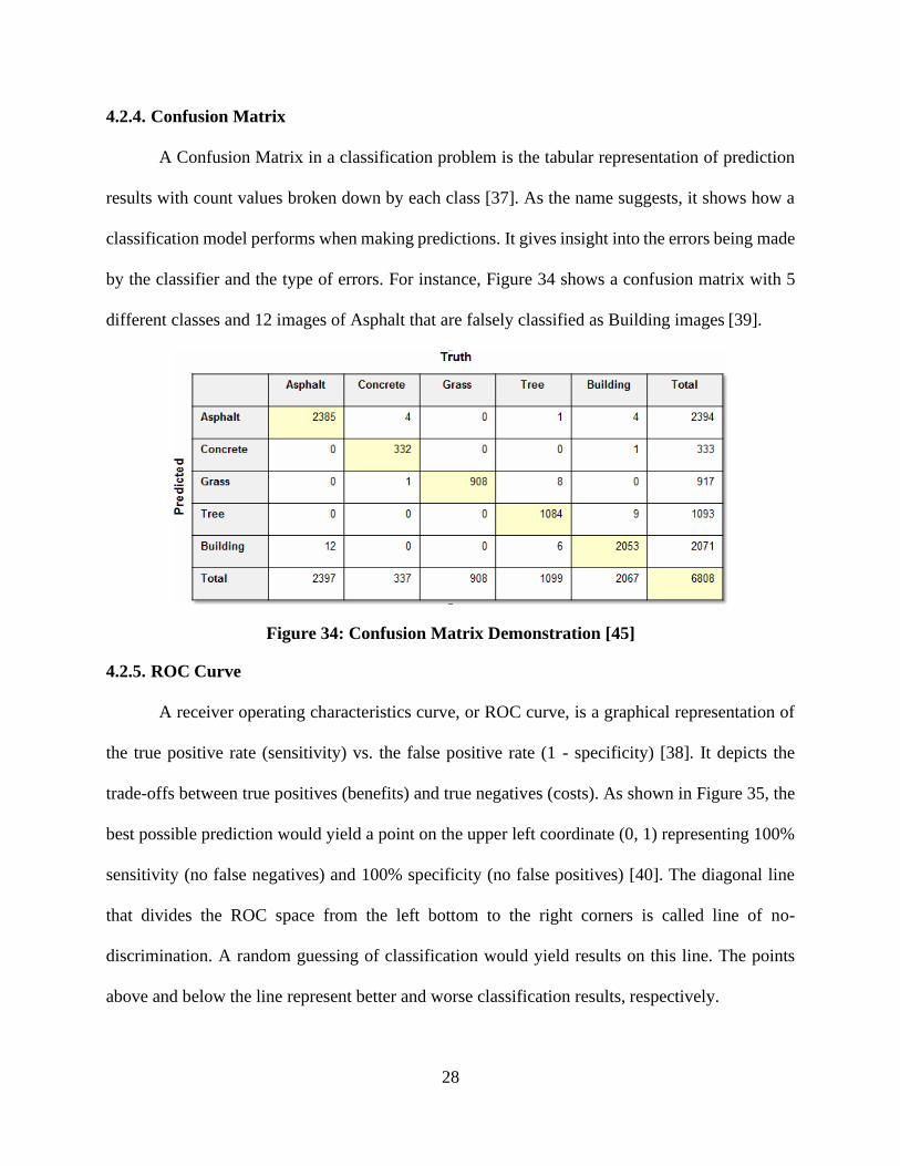
4.2.4. Confusion Matrix
A Confusion Matrix in a classification problem is the tabular representation of prediction
results with count values broken down by each class [37]. As the name suggests, it shows how a
classification model performs when making predictions. It gives insight into the errors being made
by the classifier and the type of errors. For instance, Figure 34 shows a confusion matrix with 5
different classes and 12 images of Asphalt that are falsely classified as Building images [39].
Figure 34: Confusion Matrix Demonstration [45]
4.2.5. ROC Curve
A receiver operating characteristics curve, or ROC curve, is a graphical representation of
the true positive rate (sensitivity) vs. the false positive rate (1 - specificity) [38]. It depicts the
trade-offs between true positives (benefits) and true negatives (costs). As shown in Figure 35, the
best possible prediction would yield a point on the upper left coordinate (0, 1) representing 100%
sensitivity (no false negatives) and 100% specificity (no false positives) [40]. The diagonal line
that divides the ROC space from the left bottom to the right corners is called line of no-
discrimination. A random guessing of classification would yield results on this line. The points
above and below the line represent better and worse classification results, respectively.
Page 39
29
Figure 35: ROC Curve Example [40]
4.3. Three Methodologies of Classification
4.3.1. Pre-trained CNN Model as Feature Extractor
Freeze all the convolution layers using the python libraries and use the pre-trained network
as just for feature extraction of the images.
The output is as shown in Figure 36. It shows all the layers are frozen as expected. The last
activation feature map is the output from ‘block5_pool’ that gives the bottleneck features. All the
training and validation dataset features are extracted, flattened and fed as input to the classifier.
Build a classifier that takes the flattened bottleneck features as input and performs the
classification. Train the model using ‘model.fit’ selecting the number of epochs, batch size,
training data and validation data. Save the model to use for classifying the testing images.
model.save(‘chest_xray_fulldataset/NORMAL_PNEUMONIA_tlearn_basic_cnn.h5’)
Page 40
30
Figure 36: Illustration of Frozen Layers
4.3.2. Pre-trained CNN Model as a Feature Extractor with Image Augmentation
Perform image augmentation on training and validation datasets. We keep layers of CNN
network frozen and generate image data using python library ‘ImageDataGenertor’. Build training
model on the data generators rather on the bottleneck features as in Method 1. Save the model as
h5 file to be used for classifying the training data.
model.save(‘chest_xray_fulldataset/NORMAL_PNEUMONIA_tlearn_img_aug_cnn.h5’)
Page 41
31
4.3.3. Pre-trained Model with Fine-Tuning and Image Augmentation
Unfreeze the last two layers – ‘block5_conv1’ and ‘block4_conv1’.
for layer in cnn_model.layers:
if layer.name in [‘block5_conv1’,
‘block4_conv1’]: set_trainable = True
if set_trainable:
layer.trainable
= True
else:
layer.trainable = False
Figure 37 describes that the block4 and block5 are now trainable backwards after each
epoch. Use the same model with the Image generators as in Section 4.1.2 to train the model. Save
the model for classifying the testing data.
model.save(‘chest_xray_fulldataset/NORMAL_PNEUMONIA_tlearn_finetune_img_aug_cnn.h5’)
Plot the changes of the validation accuracy after each epoch. Load the test images. Scale
them, split the labels and save them to separate lists. Load the ‘.h5’ file and input the test data to
get the classification. Choose random test images and show their actual and predicted labels. Plot
confusion matrix that shows the True Normal and True Pneumonia classification. Calculate the
accuracy, precision, sensitivity, specificity and F-1 score. Create a 2d array with all the accuracies
updated to it. Visualize it as a DataFrame and plot the bar diagram of all accuracies for each pre-
trained network.
Page 42
32
Figure 37: Illustration of Unfrozen Layers for Fine-tuning
Page 43
33
4.4. Evaluation Results
4.4.1. Random Test Images Classification
Choose random images from test dataset. The image can be either ‘NORMAL’ or
‘PNEUMONIA’. Classify the image using the pre-trained models and plot the image with its actual
label and predicted label. Figure 38 describes the random generation of test images and their
classification using the VGG16 model with Image Augmentation and Fine-Tuning method.
Figure 38: Classified Images
Page 44
34
4.4.2. Accuracy
The prediction accuracies of all pre-trained networks with the corresponding method of the
classification is listed in Table 5. From the three approaches used, Feature Extraction with Image
Augmentation gave the best results, out of which the ‘Xception’ model achieved the best accuracy
with 92.5%. Figure 39 shows the bar plot visual of all accuracies.
Table 5: Accuracy Results
Model Conv Method Image Augm Fine Tuning
VGG16 84.75 92.15 87.17
VGG19 76.118 91.42 88.52
ResNet50 79.82 90.11 63.17
InceptionV3 78.217 88.521 68.04
Xception 83.594 92.57 67.46
DenseNet 81.56 88.98 56.66
Figure 39: Bar plot of Accuracy Values Obtained
Page 45
35
4.4.3. Precision
As Precision describes the true Pneumonia images out of predicted Pneumonia, Table 6
and Figure 40 represents the percentage measures of the same. From the three approaches, the
Feature Extraction with Image Augmentation gave the best results, out of which the ‘VGG16’
model achieved the best precision value of 94.55%. Figure 40 shows the bar plot visual of all the
precision.
Table 6: Precision Results
Model Conv Method Image Augm Fine Tuning
VGG16 90.66 94.559 90.45
VGG19 84.16 93.5 94.1
ResNet50 89.68 93.42 76.07
InceptionV3 85.26 90.95 80.16
Xception 89.7 94.11 81.57
DenseNet 88.28 92.4 77.16
Figure 40: Bar Plot of Precision
Page 46
36
4.4.4. Recall/Sensitivity
As Sensitivity is the probability of being tested positive when the disease is present, Table
7 and Figure 41 represents the results of the test to correctly classify an individual as ‘diseased’.
From the three approaches used in this paper, Feature Extraction with Image Augmentation gave
the best results, out of which the ‘Xception’ model achieved the best Sensitivity of 94.35%.
Table 7: Recall/Sensitivity Results
Model Conv Method Image Augm Fine Tuning
VGG16 87.17 93.58 87.43
VGG19 81.79 92.3 90
ResNet50 80.25 91.02 73.06
InceptionV3 83.07 90.25 76.66
Xception 87.17 94.35 77.17
DenseNet 88.07 90.51 75.38
Figure 41: Bar Plot of Sensitivity
Page 47
37
4.4.5. Specificity
As Specificity is the probability of being tested negative when the disease is not present,
Table 8 and Figure 42 represents the results of the test to correctly classify an individual as ‘not
diseased’. From the three approaches used, Feature Extraction with Image Augmentation gave the
best results, out of which the ‘VGG16’ model achieved the best Specificity of 93%.
Table 8: Specificity Results
Model Conv Method Image Augm Fine Tuning
VGG16 88.33 93 88
VGG19 80 91.66 92.66
ResNet50 88 91.66 71
InceptionV3 81.33 88.33 75.33
Xception 87 92.33 77.33
DenseNet 85.66 90.33 71
Figure 42: Bar Plot of Specificity
Page 48
38
4.4.6. F1-score
As the dataset classes distribution are unbalanced, the F-1 score shows the better accuracy
values compared to normal accuracy measured. From the three approaches used in this paper,
Feature Extraction with Image Augmentation gave the best results, out of which the ‘VGG16’
model achieved the best F1-Score of 94%. Table 9 and Figure 43 shows the DataFrame and Bar
plot visual of F1-scores.
Table 9: F1-Score Results
Model Conv Method Image Augm Fine Tuning
VGG16 88.33 94 88
VGG19 82 92.66 92.66
ResNet50 84 92.66 74
InceptionV3 84.33 90.33 78.33
Xception 88 93.75 79.33
DenseNet 85.66 91.33 76
Figure 43: Bar Plot of F1-Score
Page 49
39
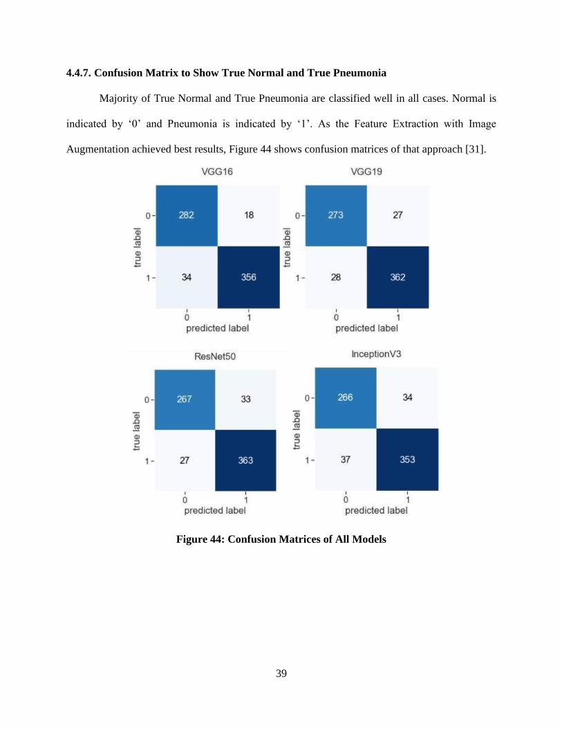
4.4.7. Confusion Matrix to Show True Normal and True Pneumonia
Majority of True Normal and True Pneumonia are classified well in all cases. Normal is
indicated by ‘0’ and Pneumonia is indicated by ‘1’. As the Feature Extraction with Image
Augmentation achieved best results, Figure 44 shows confusion matrices of that approach [31].
Figure 44: Confusion Matrices of All Models
Page 50
40
Figure 44: Confusion Matrices of All Models (continued)
4.4.8. ROC Curve for Best and Worst Model
Figure 45 describes the Receiving Operating Characteristic curve for the best and worst
models, respectively [32].
Figure 45: ROC Curve
Page 51
41
5. CONCLUSION
The project work compares the performance of six pre-trained convolutional neural
networks with three types of approaches, namely CNN as feature extraction, CNN as feature
extraction with image augmentation, and CNN with fine-tuning and image augmentation. The
dataset includes chest X-rays of Normal and Pneumonia patients.
With the help of transfer learning and the approaches mentioned above, better accuracy
values are achieved with almost all the pre-trained networks for the classification of medical
images. In all the pre-trained networks used, Feature extraction with Image augmentation method
delivered the best results. Of all the networks the ‘Xception’ model with Image Augmentation as
feature extraction method returned the highest accuracy of 92.5% followed by VGG16, VGG19,
ResNet 50, InceptionV3 and DenseNet201 with 92.1%, 91.42%, 90%, 88% and 88%, respectively.
The same method showed better indication in terms of Sensitivity where as the ‘VGG16’ model
showed better results in specificity, precision, recall and F1 score. Hence, when the datasets are
balanced and unbalanced, the Feature Extraction with Image Augmentation approach with the pre-
trained networks ‘Xception’ and ‘VGG16’ performed well respectively.
Page 52
42
REFERENCES
[1] “Computer Colors (RGB).” Smile Basic, last accessed: June 2020,
http://smilebasic.com/en/e-manual/manual28/.
[2] V. Nigam, “Understanding Neural Networks. From neuron to RNN, CNN, and Deep
Learning”, 2018, https://towardsdatascience.com/understanding-neural-networks- from-
neuron-to-rnn-cnn-and-deep-learning-cd88e90e0a90.
[3] Stanford.edu, “Multi-Layer Neural Network”, 2020,
http://ufldl.stanford.edu/tutorial/supervised/MultiLayerNeuralNetworks/.
[4] Isikdogan, “Transfer Learning”, 2018, http://www.isikdogan.com/blog/transfer-
learning.html.
[5] N. Donges, “What is Transfer Learning? Exploring the popular deep learning approach”,
2019, https://builtin.com/data-science/transfer-learning.
[6] P. Radhakrishnan, “What is Transfer Learning?”, 2017,
https://towardsdatascience.com/what- is-transfer-learning-8b1a0fa42b4.
[7] TensorFlow, “Transfer learning and fine-tuning”, 2020,
“https://www.tensorflow.org/tutorials/images/transfer_learning”.
[8] Hackerearth, “ Transfer Learning”, https://www.hackerearth.com/practice/machine-
learning/transfer-learning/ transfer-learning-intro/tutorial/, last accessed: June 2020.
[9] J. Brownlee, “A gentle introduction to Transfer Learning for Deep Learning”, 2017,
https://machinelearningmastery.com/transfer-learning-for-deep-learning/.
[10] D. S. Kermany et al., “Identifying Medical Diagnoses and Treatable Diseases by Image-
Based Deep Learning”. Cell, vol. 172, no. 5, pp. 1122-1131, Feb. 2018.
Page 53
43
[11] O. Stephen et al., “An Efficient Deep Learning Approach to Pneumonia Classification in
Healthcare”. Hindawi, Journal of Healthcare Engineering , vol. 2019, Mar. 2019.
[12] H. Wu et al., “Predict pneumonia with chest X-ray images based on convolutional deep
neural learning networks”. Journal of Intelligent and Fuzzy Systems, vol: Pre-press, no.
Pre-Press, pp. 1-15, 2020.
[13] G. Liang and L. Zheng. “A transfer learning method with deep residual network for
pediatric pneumonia diagnosis”. Computer Methods and Programs in Biomedicine, vol.
187, June 2019.
[14] M. B. Rodrigues et al., “Health of things algorithms for malignancy level classification of
lung nodules”. IEEE Xplore, vol. 6, Apr 2018.
[15] S. Ruder, “Transfer Learning-Machine Learning’s Next Frontier”, 2017,
https://ruder.io/transfer-learning/.
[16] S. Pokhrel, “How does Computer understand Images?”, 2019,
https://towardsdatascience.com/how-does-computer-understand-images-
c1566d4537bf#:~:text=A%20computer%20sees%20an%20image%20as%200s%20and%
201s.,smallest%20unit%20in%20an%20image.&text=As%20shown%20in%20the%20ab
ove,com puter%20can%20understand%20the%20image.
[17] Wikipedia. “https://en.wikipedia.org/wiki/RGB_color_model”, last accessed: June 2020.
[18] D. Upadhyay, “How a computer looks at pictures: Image Classification”, 2019,
https://medium.com/datadriveninvestor/how-a-computer-looks-at-pictures-image-
classification-a4992a83f46b
Page 54
44
[19] A. Rao, “Convolutional Neural Network Tutorial (CNN) – Developing An Image
Classifier In Python Using TensorFlow”, 2019,
https://www.edureka.co/blog/convolutional-neural-network/
[20] D. Liu. “A Practical Guide to ReLU, Start using and understanding ReLU without BS or
fancy equations”, 2017, https://medium.com/@danqing/a-practical-guide-to-relu-
b83ca804f1f7.
[21] Missinglink, “Fully Connected Layers in Convolutional Neural Networks: The Complete
Guide”, last accessed: June 2020, https://missinglink.ai/guides/convolutional-neural-
networks/fully-connected- layers-convolutional-neural-networks-complete-guide/.
[22] D. S. Gupta,“ Transfer learning and the art of using Pre-trained Models in Deep
Learning”, 2017, https://www.analyticsvidhya.com/blog/2017/06/transfer- learning-the-
art-of-fine-tuning-a-pre-trained-model/.
[23] Google Cloud, “Advanced Guide to Inception v3 on Cloud TPU”, 2020
“https://cloud.google.com/tpu/docs/inception-v3-advanced”.
[24] S. Tsang, “ Review: Inception-v3 — 1st Runner Up (Image Classification)”, 2018,
https://medium.com/@sh.tsang/review-inception-v3-1st-runner-up-image-classification-
in- ilsvrc-2015-
17915421f77c#:~:text=With%20multi%2Dmodel%20multi%2Dcrop,which%20will%20
be% 20reviewed%20later.
[25] R. Karim, “Illustrated: 10 CNN Architectures. A compiled visualisation of the common
convolutional neural networks”, 2019, https://towardsdatascience.com/illustrated-10-
cnn-architectures-95d78ace614d.
Page 55
45
[26] P. Marcelino, “Transfer learning from pre-trained models”, 2018,
https://towardsdatascience.com/transfer-learning-from-pre-trained-models-f2393f124751.
[27] Q. Guan, “Deep convolutional neural network VGG-16 model for differential diagnosing
of papillary thyroid carcinomas in cytological images: a pilot study”, 2019,
https://www.ncbi.nlm.nih.gov/pmc/articles/PMC6775529/.
[28] Keras, “Keras Applications”, Last accessed: June 2020,
“https://keras.io/api/applications/”.
[29] D. Sarkar. “A Comprehensive Hands-on Guide to Transfer Learning with Real-World
Applications in Deep Learning”, 2018, https://towardsdatascience.com/a-
comprehensive-hands-on-guide-to-transfer-learning-with-real-world-applications-in-
deep-learning-212bf3b2f27a.
[30] R. Gour, “ Transfer Learning for Deep Learning with CNN”. 2018,
https://medium.com/@rinu.gour123/transfer-learning-for-deep-learning-with-cnn-
afa1fe0aa7e2.
[31] Scikit learn. “https://scikit-learn.org/stable/modules/generated/
sklearn.metrics.confusion_matrix.html”, last accessed: June 2020.
[32] S. S. Nazrul, “Receiver Operating Characteristic Curves Demystified (in Python)”, 2018,
https://towardsdatascience.com/receiver-operating-characteristic-curves-demystified-in-
python-bd531a4364d0.
[33] “Sensitivity and specificity.”, Wikipedia, Wikimedia Foundation, last accessed: June
2020, https://en.wikipedia.org/wiki/Sensitivity_and_specificity.
[34] “Precision and recall”, Wikipedia, Wikimedia Foundation, last accessed: July 2020,
https://en.wikipedia.org/wiki/Precision_and_recall.
Page 56
46
[35] “F1 score“, Wikipedia, Wikimedia Foundation, last accessed: June 2020,
https://en.wikipedia.org/wiki/F1_score.
[36] K. P. Shung, “Accuracy, Precision, Recall or F1?”, 2018,
https://towardsdatascience.com/accuracy-precision-recall-or-f1-331fb37c5cb9.
[37] “Confusion Matrix.” Wikipedia, Wikimedia Foundation, last accessed: June 2020.
https://en.wikipedia.org/wiki/Confusion_matrix.
[38] W. Zhu. “Sensitivity, Specificity, Accuracy, Associated Confidence Interval and ROC
Analysis with Practical SAS Implementations”, 2010,
https://www.lexjansen.com/nesug/nesug10/hl/hl07.pdf, NESUG.
[39] S. Narkade, “Understanding Confusion Matrix”. 2018,
https://towardsdatascience.com/understanding-confusion-matrix-a9ad42dcfd62.
[40] “Receiver Operating Characteristics.” Wikipedia, Wikimedia Foundation, last accessed:
June 2020, https://en.wikipedia.org/wiki/Receiver_operating_characteristic.
[41] R Yamashita et al., “Convolutional neural networks: an overview and application in
radiology”, Springer, June 2018, https://link.springer.com/article/10.1007/s13244-018-
0639-9 .
[42] R Karim, “Illustrated: 10 CNN Architectures”, 2019,
https://towardsdatascience.com/illustrated-10-cnn-architectures-95d78ace614d.
[43] A Joshi, “How to leverage transfer learning using pretrained CNN models”, 2019,
https://hub.packtpub.com/how-to-leverage-transfer-learning-using-pretrained-cnn-
models-tutorial/
[44] Gizmo, “Timer Accuracy”, 2018, https://gizmo-engineering.com/information/technical-
information/timer-accuracy/
Page 57
47
[45] Harris, “ENVIConfustionMatrix:ConfustionMatrix”, 2020,
https://www.harrsisgeospatial.com/docs/ENVIConfustionMatrix_ConfustionMatrix.html.