Image coding by multistep, adaptive flux interpolation

L. Baghai-Ravary S.W. Beet M .O. To kh i

Indexing terms: Image coding, Adaptive flux interpolation, Multistep adaptive flux interpolation

Abstract: The authors describe and discuss the new technique, multistep adaptive flux interpolation (MAFI), and its application to image data for coding. When applied to an image, MAFI produces an output which is also in an image form, but which has a more uniform feature density and a greatly reduced size. MAFI warps the input image by removing those rows and columns which contain a majority of redundant pixels. The side information required for reconstruction is minimal, and the image can be further compressed using conventional coders, making the compression ratio even higher. Because of its warped nature, the MAFI output’s statistics are also more consistent with the properties assumed by block-based discrete cosine transform (DCT) methods.

1 Introduction

Methods based on the two-dimensional discrete cosine transform (DCT) [l], such as that specified by JPEG (Joint Photographic Image Expert Group) [2] , generally use the same vector quantisation process for all parts of the image. Thus, they inherently assume that the data statistics are uniform, but in many cases this is not true, as different parts of the image may exhibit very different feature densities. However, if the image were warped before being encoded, the assumption of uni- formity could be made more realistic. An arbitrary two-dimensional warping function could be applied, but this would require something of the order of one bit per pixel to specify the proximity of each encoded pixel to its neighbours in each direction. Such a high level of side information would be prohibitive. A more practical solution is to identify and remove the whole of any columns or rows which are redundant.

The redundant columns and rows in a (two- dimensional) image contain data which could be interpolated from their neighbours. Provided the interpolation algorithm is sophisticated enough, and

0 IEE, 1996 IEE Proceedings online no. 19960576 Paper first received 12th July 1995 and in revised form 25th April 1996 L. Baghai-Ravary and S.W. Beet were with the University of Sheffield and are now with Aculab plc, Lakeside, Bramley Road, Mount Farm, Milton Keynes MK1 IPT, UK M.O. To& is with the Department of Automatic Control and Systems Engineering, The University of Sheffield, Mappin Street, Sheffield S1 3JD, UK

the same features are present in all those columns or rows, the neighbours need not be very similar to one another, or to the data being interpolated. Image compression can be achieved by removing this redundant data. Removal of complete columns and rows leaves the data in the form of a reduced dimensionality image (with minimal side information) which can be further compressed by DCT and other algorithms [3, 41. This technique improves on the compression ratio and modifies the image statistics, producing a more uniform distribution of spatial frequencies over the image.

Furthermore, image compression by localised warp- ing, as described here, can be applied repeatedly, yield- ing additional compression with each application. This is in contrast to other image coders such as JPEG, which produce outputs which are different in form from that of their inputs and cannot be viewed as an image, directly. Thus these compression algorithms can only be applied once to any image.

2 Compression process

Adaptive flux interpolation (AFI) is a powerful method for interpolating a vector from a sequence [5, 61. Multi- step AFI (MAFI) uses the same model to interpolate a sequence of vectors and can be used to identify extended sequences of vectors which are redundant. For simplicity, only the MAFI algorithm is discussed further here (see the next Section), but the AFI algo- rithm is simply a special case of this, where every block to be interpolated is of fixed length (one vector).

By treating the image as a matrix with its columns as vector inputs to MAFI, the redundant columns can be removed. The output of the MAFI process is in a compressed form, which consists of the remaining columns concatenated, together with a set of numbers recording interpolated block sizes to allow reconstruction of the image. The image is, therefore, of a reduced horizontal dimensionality while still maintaining an image form.

This reduced image matrix can be transposed, and then the whole process reapplied to remove the redun- dant rows. Further redundancy can be removed by repeating this process one or more times (see Fig. 1).

compressed input image - 4 z + - - J @ z d e d image image

Fig. 1 Encoding system

IEE Proc.-Vis. Image Signal Process., Vol. 143, No. 6, December 1996 331

3

Multistep adaptive flux interpolation (MAFI) is analo- gous to optical flow [7, 81, as both techniques are used for tracking features in an image. However, MAFI functions in a two-dimensional image space, whereas optical flow is used for image sequences which are effectively three-dimensional.

MAFI assumes that lines of flux can be defined within an image, joining pixels of similar values. At least one line of flux passes through every pixel in the image, linking it to related pixels in neighbouring col- umns or rows. A complete image can then be defined in terms of lines of flux and the variation in image intensity along them. In many images, that variation is much smaller and smoother than the variation between horizontally or vertically adjacent pixels. This means that the pixels joined by each line can be reconstructed without reference to every corresponding pixel of the original image: many can be omitted and later recon- structed by interpolation along the lines of flux.

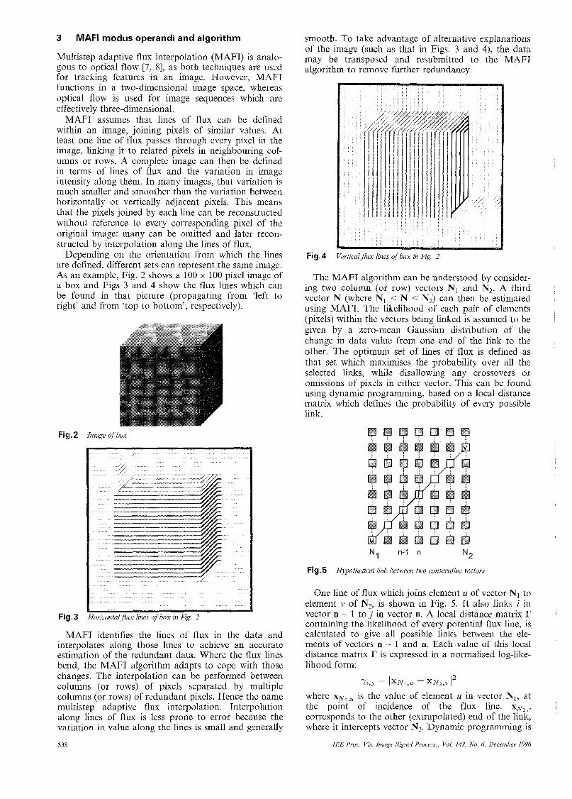
Depending on the orientation from which the lines are defined, different sets can represent the same image. As an example, Fig. 2 shows a 100 x 100 pixel image of a box and Figs 3 and 4 show the flux lines which can be found in that picture (propagating from ‘left to right’ and from ‘top to bottom’, respectively).

MAFI modus operandi and algorithm

Fig.2 Image of box

Fig.3 Horizontalflun lines of box in Fig 2

MAFI identifies the lines of flux in the data and interpolates along those lines to achieve an accurate estimation of the redundant data. Where the flux lines bend, the MAFI algorithm adapts to cope with those changes. The interpolation can be performed between columns (or rows) of pixels separated by multiple columns (or rows) of redundant pixels. Hence the name multistep adaptive flux interpolation. Interpolation along lines of flux is less prone to error because the variation in value along the lines is small and generally

338

smooth. To take advantage of alternative explanations of the image (such as that in Figs. 3 and 4), the data may be transposed and resubmitted to the MAFI algorithm to remove further redundancy.

111 II

Fig.4 Verticalflux lines of box in Fig. 2

The MAFI algorithm can be understood by consider- ing two column (or row) vectors N1 and N2. A third vector N (where Nl < N < N2) can then be estimated using MAFI. The likelihood of each pair of elements (pixels) within the vectors being linked is assumed to be given by a zero-mean Gaussian distribution of the change in data value from one end of the link to the other. The optimum set of lines of flux is defined as that set which maximises the probability over all the selected links, while disallowing any crossovers or omissions of pixels in either vector. This can be found using dynamic programming, based on a local distance matrix which defines the probability of every possible link.

Q g @ Q g g g \ \ ! \ I ; :

N2 N, n-I n

Fig. 5 Hypothetical link between two consecutive vectors

One line of flux which joins element U of vector NI to element v of N2, is shown in Fig. 5. It also links i in vector n - 1 to j in vector n. A local distance matrix r containing the likelihood of every potential flux line, is calculated to give all possible links between the ele- ments of vectors n - 1 and n. Each value of this local distance matrix r is expressed in a normalised log-like- lihood form:

Y2,J = lXNl,U - XNZ,Vl2

where x ~ , , ~ is the value of element U in vector NI, at the point of incidence of the flux line. x N ~ , ~ corresponds to the other (extrapolated) end of the link, where it intercepts vector N2. Dynamic programming is

IEE Proc -Vis Image Signal Process, Vol 143, No 6, December 1996

Fig. 6 Moon landing

Original image (left) and reconstructed image after two applications of MAFI (right), without visual acceptability constraints:

Compression ratio = 42%

then used to find the set of flux lines which give the maximum total log-likelihood over all possible combinations of lines.

The use of dynamic programming to identify this mathematically optimal set of links also allows the imposition of arbitrary constraints to ensure that any interpolation is performed in a visually acceptable fashion. In particular, very oblique lines are visually distracting, so these can be disallowed by setting the respective elements of the local distance matrix to infinity.

The redundant vectors (columns or rows) are identi- fied by successively attempting to encode blocks of increasing numbers of vectors, until a normalised meas- ure of the root mean square error exceeds a threshold. At this point, the last vector in the block N2 is trans- mitted, together with a number giving the size of the block N2 - NI. The threshold is chosen to give the desired image quality.

In the box example (Fig. 2) the original 100 x 100 pixel image can be reduced to only 36 pixels. plus a minimum of side information, which together carry all the necessary material for reconstruction of that image [Note I]. The number of pixels retained is independent of the shape or the size of the box, or the size of the picture as a whole, although the side information very slightly increases with the width and height of the picture. This picture is simple and very geometrical. Thus after compression, it can be reconstructed with no error. The 36 pixels are from the points where the vertical and horizontal critical flux lines intersect; these lines are along the vertical and horizontal: (i) edges of the picture (two of each); (ii) visible edges of the box (three of each); (iii) hidden edges of the box (one of each). So there are six vertical and six horizontal critical flux lines overall, intersecting at 36 points.

4 Coding considerations

The degree of compression possible with MAFI depends on several factors. These are outlined below.

4.7 Acceptable level of image distortion The value of the threshold, used to distinguish between the critical and the predictable vectors in the image, determines the level of maximum distortion which is allowed to be present in the data after reconstruction. The higher the threshold, the more data is perceived as Note 1: In this example, a maximum of 60 bits is required to encode the five vertical and five horizontal block sizes with six bits per block. With more sophisticated encoding algorithms, and with a more ‘normal’ image, the block sizes can be encoded with around two bits per block (equivalent to le* bits per pixel or less).

being redundant and, thus, the higher the compression ratio.

4.2 Nature of the image An image with a low average feature density gives a higher compression ratio than an image dominated by a higher feature density. Fine details contain more crit- ical information and are therefore, less predictable than gross features. However, the shape and structure of the features also influences the final compression. For example, an image containing only combed hair is compressed more than one containing very curly or fuzzy hair.

4.3 ‘Visual acceptability ’ constraints during dynamic programming As mentioned earlier, dynamic programming (DP) is used to match and link similar pixels of the columns together, to yield the flux lines. A limit is set in the DP routine so that this procedure is carried out reasonably and unrealistic links, such as a very sharp one from one end of one column to the other end of the next, cannot be made. This type of link is not usually visually acceptable in an image and is, therefore, disallowed.

The freedom of the feature to match and link from one column to another is, thus, fixed by a limit param- eter. If this limit is set too high the reconstructed data may contain unrealistic and visually unacceptable dis- tortions. This is especially noticeable if the known frames are widely separated, and in practice, the fur- ther apart these frames are, the smaller the limit must be to obtain reliable interpolation.

Examples of unacceptable links are shown in the high compression ratio images in Figs. 8 and 10. The reconstructed images were produced with no limit on the allowed links, and show occasional spurious lines joining unrelated points in the image. The other images are relatively unaffected because of the more moderate compression ratios (Figs. 6 and 7) or the nature of the image (Fig. 9). However, in general, the likelihood of such lines appearing is increased when high compres- sion ratios are attempted. At the other extreme, if the limit is set too low, it could restrict the interpolator’s ability to create valid links, and may result in low com- pression ratios because the pixels may not be able to be matched correctly.

4.4 Number of MAFI applications and their directions MAFI can be applied several times without lowering the standard of allowable error in the reconstructed data (set by the threshold) provided each application is at a different orientation from its predecessor. This, in

339 IEE Proc-Vis. Image Signal Process., Vol. 143, No. 6, December 1996

Fig. 7 Man in front of building Compression ratio = 60%

Original image (left) and reconstructed image after two applications of MAFI (right), without visual acceptability constraints:

Fig. 8 Statue of Liberty Compression ratio = 75%

Original image (left) and reconstructed image a$er two applications of MAFI (right), without visual acceptability constraints:

Fig.9 Some keys Compression ratio = 91%

Original image (left) and reconstructed image after two applications of MAFI (right), without visual acceptability constraints.

Fig. 10 A toucan Compression ratio = 97%

Original image (le$) and reconstructed image after two applications

fact, further increases the compression ratio on each application.

In this paper, and for the sake of simplicity, MAFI is onentated orthogonally on each application to remove the redundant rows and columns in the data. However, it is not necessary that the adjustment should be orthogonal, as long as it is at a different angle to its

of MAFI (right), without visual acceptability constraints:

previous application. Fig. 11 shows another method for utilising MAFI. Here, MAFI is applied in four direc- tions, each 45" to the other (from left to right, respec- tively; the arrow shows the direction of MAFI application). This technique will not only remove the predictable rows and columns, but also any predictable diagonal vectors. The only drawback to this approach

340 IEE Proc -Vis Image Signal Process, Vol 143, No 6, December 1996

is that the rectangular image format is lost and so the MAFI output would be difficult to encode further.

Fig. 11 direction of MAFI application

MAFI applied in four nonorthogonal directions Arrow shows

output of output of first MAFI second MAFI application, application in the same direction

1 3 y v 3 3 1 m 3 . m .

3 q o 3 e * i i 1 i i* s o * * 3 o i * 3 3 ! * * o Q O d o b o b c j i i i i 3 i 3

133Q1331+ i o * + ii

3 3 Fig. 12 Consequences of applying MAFI in same direction twice

It is not practical to apply MAFI in the same direc- tion, consecutively. This would have a similar effect to an increase in the threshold on the former application and could give suboptimal results (Fig. 12).

The compression ratio increases with each applica- tion of MAFI, although if it is applied too many times successive increases become smaller and eventually reach zero when all redundant pixels have been removed. The number of times MAFI is usefully applied depends on the nature of the image, the thresh- old and the DP limit settings (i.e. on the quality and desired characteristics of the reconstructed image).

4.5 Changes in the MAFI parameters between applications The parameters include: threshold, DP limit, and the direction of application. The structure and the nature of the output of each MAFI application are different from those of its input. For example, the output would have a higher feature density, where redundancy has been detected, and dimensionally it is reduced in size. Consequently, better results could be obtained by changing the MAFI parameters for each application to match the properties of the respective input images, and achieve an optimal result.

However, in practice, it is the characteristics of the original image which have the greatest effect on the choice of parameters. It is possible to achieve good lev- els of performance with just a single set of parameters for multiple applications, provided the direction of application is changed each time.

5 Experiments

A number of experiments have been conducted to eval- uate the optimum parameters and to observe how criti- cal their values are to the resulting image quality. MAFI has been applied a number of times in orthogo- nal directions and the signal-to-noise ratio (SNR) of the reconstructed image evaluated. The results of these experiments are summarised in Figs. 13 and 14.

Fig. 13 shows the variation in compression ratio with the value of the DP limit (for a range of coding error thresholds and numbers of MAFI applications). The value of the limit parameter is numerically equal to the gradient of the steepest line of flux plus one. The opti- mum value of this parameter varies from image to image, but for the data used here, it is clear that there is an optimum limit value of 2 (a maximum gradient of

IEE Proc.-Vis. Image Signal Process., Vol. 143, No. 6 , December 1996

+1). This value is much more critical (and image- dependent) when only one MAFI application is used, while multiple applications provide broadly compara- ble levels of compression over a range of limit values. In general, the optimum limit is still the same, but it is less critical to the compression. This is because, although the shorter blocks, which result from allowing unrealistic flux linkages during the first application, leave a higher level of redundancy in the image, that redundancy is in a form which can be removed easily in the orthogonal direction. That is to say that any fea- tures with a gradient greater than 21 in the original direction will have a gradient less than that in the orthogonal direction.

1oor thre?hold /."'... .. - ............. - _ _ ~ - - ~ ---... .................................... 1 -I -------------- -___ -___ _________-----

901- I

8 0 1 f i - 3 500'0 ,-" 70t

50 a

.>---".. ............ ................ ._______ ......................... .__-__ -- -_____ _ _ _ _ -____ _ _ _ _ -. --_---- /* ..

l o t

0 5 10 N value of DP limit

Compression ratio as function of DP gradient limit Fig. 13 Number of applications: 4 .."; 3 - - -; 2 - - -: 1 ~

30 r

0 0 20 40 60 80 100

compression,% Fig. 14 Signal-to-noise ratio as function of compression ratio

Fig. 14 shows the relationship between compression ratio and SNR for different numbers of MAFI applica- tions, with the limit set to 2. This graph is, however, virtually identical for other values of the limit. The coding error threshold has been varied to achieve the different SNRs and compression ratios. It should be

341

noted here that this graph highlights the inappropriate- ness of SNR as a measure of perceived quality. The nature of the distortion introduced by MAFI coding appears quite severe from the values presented in Fig. 14, but when observing the quality of the recon- structed images in Figs. 15-18, for example, it can be seen that that distortion is not visually significant. However, the development of a more meaningful meas- ure (which could allow for the shape, intensity, texture and visual context of the features in an image) is itself the subject of ongoing research.

Fig. 15 Original image (face of clown)

Fig. 16 MAFI

Reconstructed image (face of clown) after two applications of

Fig. 17 MAFI

Reconstructed image (face of clown) after four applications of

Figs. 15-18 show a rendition of the MATLAB clown, which contains large amounts of fine detail and texture. Thus this is quite a difficult image, chosen to illustrate the nature of the distortion introduced by MAFI coding, rather than typical values for its performance. Even so, MAFI can remove around two- thirds of the data with four applications. The compression achieved after each MAFI application is

342

shown in Table 1. This Table shows both the compression achieved with MAFI alone, and that when MAFI is followed by JPEG coding [Note 21. For reference, the row labelled as using zero applications of MAFI shows the compression for JPEG alone. In this Table, the compression is quoted as a percentage, rather than giving (for example) the number of bits per pixel, since the MAFI algorithm will provide similar levels of compression, regardless of the number of bits per pixel in the original or the reconstructed images. Data is either transmitted ‘as is’ or discarded completely; it is not quantised and the number of bits transmitted will depend on the number of bits per pixel in the original image.

Fig. 1 8 Transmitted data after four applications of MAFI

Fig. 15 shows the original 320 x 200 image of the MATLAB clown and Figs. 16 and 17, the recon- structed versions after applying MAFI two and four times,respectively. Fig. 18 shows the final encoded image (118 x 142 pixels), after all redundant rows and columns have been removed. It is clear that the largest part of the compression has occurred on the left and the lower halves of the image. The upper right-hand corner, which contains the hair and is much more finely detailed, has not been so heavily compressed. Thus the spatial frequencies in the MAFI compressed image have become more uniform.

Table 1: Compression achieved by successive applica- tions of MAFl

Number of MAFl Compression applications (bitdpixel)

Side information

MAFl MAFl + JPEG

(%) (%) 0 0.0 67.8 0.000

0.006 59.0 84.9 1

2 68.9 87.7 0.010

3 69.8 88.1 0.01 1

4 70.5 88.2 0.012

Another item of interest is the directions of the flux linkages in a complex image of this sort. It is difficult to represent so much data graphically, so Figs. 19 and 20 show a small section of the image (including an eye and a part of the nose), and the lines of flux, calculated horizontally, with the darkness of the lines of flux Note 2: The REG algorithm was from the Graphic Workshop 1.1 package, with a quahty factor of 75. Any incomplete 8 x 8 DCT blocks, as required for the DCT of the P E G algorithm, were discarded and the values presented in this paper, calculated based on only that part of the original image which could be reconstructed.

IEE Proc.-Vis. Image Signal Process., Vol. 143, No. 6, December 1996

denoting the darkness of the image at the respective points. The flux generally follows intuitively meaning- ful contours in the image, adapting to the shapes of the features within the image.

considered in this study, can remove more than 70% of the data without introducing unacceptable levels of distortion. The SNR at this level of compression is more than IOdB, but the distortion is not of an

Fig. 19 Detailjiom Fig. 15 (eye, nose and some hair)

Fig. 20 Adapted horizontal flux lines (eye, nose and some hair)

6 Conclusions

The development of the new algorithm MAFI has been presented and its performance in image compression has been demonstrated. It has been found that MAFI, even for detailed images such as the clown’s face

obviously structured form and is visually acceptable. This is indicative of the inappropriateness of mean square error values as a criterion of visual acceptability, when distortion is of a more complicated structure, as here.

In practice, two applications of MAFI, one in each direction, are sufficient to obtain very nearly the best compression ratio for any given SNR. They can remove the bulk of the redundant rows and columns, although some slight improvement can be obtained by further applications. However, the main advantage of using multiple orthogonal applications is not to achieve greater compression, but to make selection of optimum coding parameters less critical. This allows a single set of parameters to be applied successfully to a wide range of image types.

Furthermore, MAFI can be used before applying other coders to reduce the size of the encoded data still further. Its output (although in a compressed form) still has an image structure and is viewable and intelligible as an image in its own right. When used in conjunction with JPEG, an average reduction in encoded data by a factor of 2.7 is obtained (relative to JPEG alone).

7 References

1 ISO/TC97/SG2/WG8-ADCTG: ‘IS0 adaptive discrete cosine transform coding scheme for still image telecommunication serv- ices’ (IS0 adct-88, N640, 1988)

2 WALLACE, G.K.: ‘The JPEG still picture compression stand- ard’, Commun. A C M , 1991, 34, (4), pp. 3144

3 MATSUDA, I., ITOH, S., and UTSUNOMIYA, T.: ‘Adaptive transform image coding based on variable-shape-blocks and directional autocorrelation models’, Signal Process., 1994, TA-7,

4 CICCONI, P., LEONARDI, R., and KUNT, M.: ‘Symmetry- based image coding’. Proceedings of the VCIP-92 conference, Boston, (SPIE-1818 (3)), 1992, pp. 1312-1323

5 BAGHAI-RAVARY, L., BEET, S.W., and TOKHI, M.O.: ‘Var- iable frame-rate speech coding by adaptive-flux interpolation’, IEEE Signal Process. Lett., (submitted)

6 BAGHAI-RAVARY, L., BEET, S.W., and TOKHI, M.O.: ‘Adaptive flux interpolation, flow-based prediction, delta or deltadelta: which is best?’. Proceedings of EuroSpeech ’95, 1995

7 ADIV, G.: ‘Determining three-dimensional motion and structure from optical flow generated by several moving objects’, IEEE Trans., 1985, PAMI-7, (7), pp. 384401

8 BERGHOLM, F., and CARLSSON, S.: ‘A ‘theory’ of optical flow’, Graphic Models Image Process., 1991, 53, (2), pp. 171-188

pp. 163-166

IEE Proc.-Vis. Image Signal Process., Vol. 143, No. 6, December 1996 343