IMAGE COMPRESSION & TRANSMISSION THROUGH DIGITAL ... · Channel Equalization 47 3.1 Channel...

IMAGE COMPRESSION & TRANSMISSION

THROUGH

DIGITAL COMMUNICATION SYSTEM

A THESIS SUBMITTED IN PARTIAL FULFILLMENT OF THE

REQUIREMENTS FOR THE DEGREE OF

Bachelor of Technology

In

Electronics & Communication Engineering

By

ANTIM MAIDA SHRIKANT VAISHNAV

Roll No. : 10509015 Roll No. : 10509014

Under the Guidance of Dr. S.MEHER

Department of Electronics & Communication Engineering

National Institute of Technology

Rourkela-769008

2009


Rourkela

CERTIFICATE

This is to certify that the thesis entitled “IMAGE COMPRESSION &

TRANSMISSION THROUGH DIGITAL COMMUNICATION SYSTEM”

submitted by Shrikant Vaishnav, Roll No. 10509014 in partial

fulfillment of the requirements for the award of Bachelor of

Technology degree in Electronics & Communication Engineering at

the National Institute of Technology, Rourkela (Deemed University)

is an authentic work carried out by him under my supervision and

guidance.

To the best of my knowledge, the matter embodied in the

thesis has not been submitted to any other University/Institute for the

award of any Degree or Diploma.

Date: (Dr. S.MEHER)


Rourkela

CERTIFICATE

This is to certify that the thesis entitled “IMAGE COMPRESSION &

TRANSMISSION THROUGH DIGITAL COMMUNICATION SYSTEM”

submitted by Antim Maida, Roll No. 10509015 in partial fulfillment

of the requirements for the award of Bachelor of Technology degree

in Electronics & Communication Engineering at the National

Institute of Technology, Rourkela (Deemed University) is an

authentic work carried out by him under my supervision and

guidance.

To the best of my knowledge, the matter embodied in the

thesis has not been submitted to any other University/Institute for the

award of any Degree or Diploma.

Date: (Dr. S.MEHER)

ACKNOWLEDGEMENT

The most pleasant point of presenting a thesis is the opportunity to thank those

who have contributed their guidance & help to it. I am grateful to Deptt. Of Electronics &

Communication Engineering, N.I.T Rourkela, for giving me the opportunity to undertake

this project, which is an integral part of the curriculum in B.Tech programme at the

National Institute Of Technology, Rourkela.

I would like to acknowledge the support

of every individual who assisted me in making this project a success & I would like to

thank & express heartfelt gratitude for my project guide Dr. S.Meher, who provided me

with valuable inputs at the critical stages of this project execution along with guidance,

support & direction without which this project would not have taken shape.

I am also thankful to the staff of Deptt.

Of Electronics & Communication Engineering, N.I.T Rourkela, for co-operating with me

& providing the necessary resources during the course of my project.

SHRIKANT VAISHNAV

DATE: Roll No. 10509014

PLACE Dept. Of Electronics & Communication Engineering

National Institute of Technology, Rourkela

ACKNOWLEDGEMENT

The most pleasant point of presenting a thesis is the opportunity to thank those

who have contributed their guidance & help to it. I am grateful to Deptt. Of Electronics &

Communication Engineering, N.I.T Rourkela, for giving me the opportunity to undertake

this project, which is an integral part of the curriculum in B.Tech programme at the

National Institute Of Technology, Rourkela.

I would like to acknowledge the support

of every individual who assisted me in making this project a success & I would like to

thank & express heartfelt gratitude for my project guide Dr. S.Meher, who provided me

with valuable inputs at the critical stages of this project execution along with guidance,

support & direction without which this project would not have taken shape.

I am also thankful to the staff of Deptt.

Of Electronics & Communication Engineering, N.I.T Rourkela, for co-operating with me

& providing the necessary resources during the course of my project.

ANTIM MAIDA

DATE: Roll No. 10509015

PLACE Dept. Of Electronics & Communication Engineering

National Institute of Technology, Rourkela

ABSTRACT

Image Compression addresses the problem of reducing the amount of data required to represent the

digital image. Compression is achieved by the removal of one or more of three basic data redundancies:

(1) Coding redundancy, which is present when less than optimal (i.e. the smallest length) code words are

used; (2) Interpixel redundancy, which results from correlations between the pixels of an image; &/or

(3) psycho visual redundancy which is due to data that is ignored by the human visual system (i.e.

visually nonessential information). Huffman codes contain the smallest possible number of code

symbols (e.g., bits) per source symbol (e.g., grey level value) subject to the constraint that the source

symbols are coded one at a time. So, Huffman coding & Shannon Coding , which remove coding

redundancies , when combined with the technique of image compression using Discrete Cosine

Transform (DCT) & Discrete Wavelet Transform (DWT) helps in compressing the image data to a very

good extent.

For the efficient transmission of an image across a channel, source coding in the form of image

compression at the transmitter side & the image recovery at the receiver side are the integral process

involved in any digital communication system. Other processes like channel encoding, signal

modulation at the transmitter side & their corresponding inverse processes at the receiver side along

with the channel equalization help greatly in minimizing the bit error rate due to the effect of noise &

bandwidth limitations (or the channel capacity) of the channel.

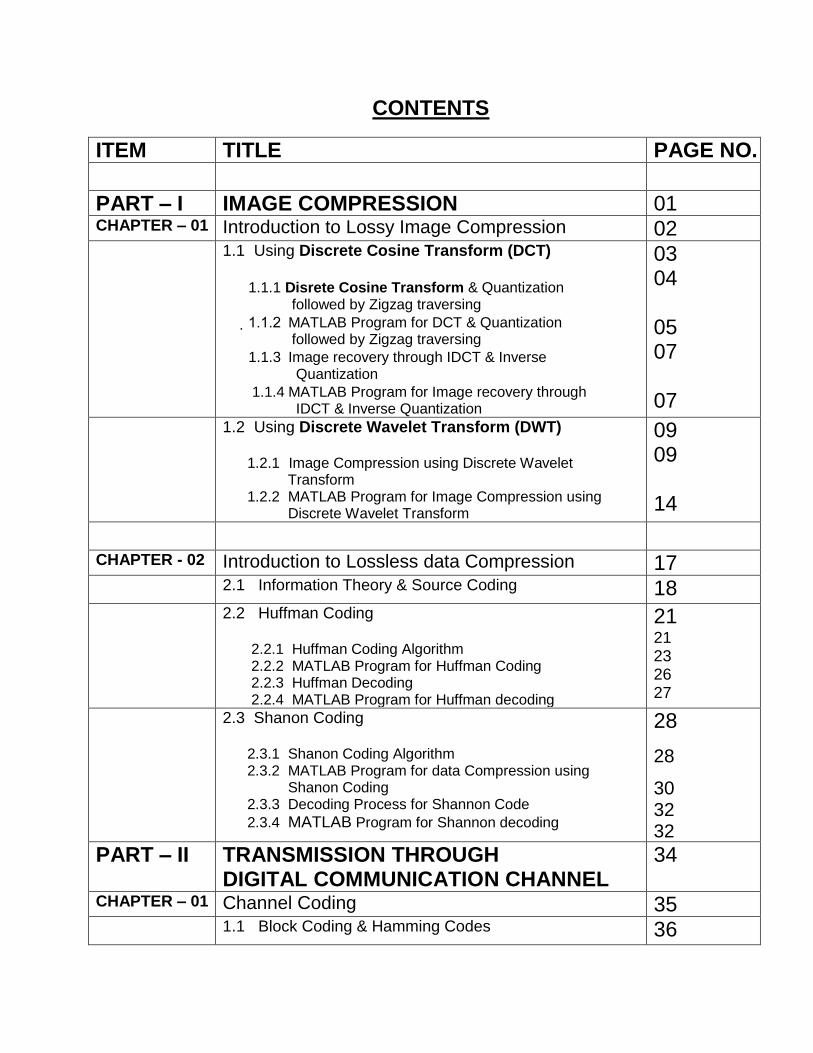
CONTENTS

ITEM TITLE PAGE NO.

PART – I IMAGE COMPRESSION 01 CHAPTER – 01 Introduction to Lossy Image Compression 02

1.1 Using Discrete Cosine Transform (DCT)

1.1.1 Disrete Cosine Transform & Quantization followed by Zigzag traversing

1.1.2 MATLAB Program for DCT & Quantization followed by Zigzag traversing

1.1.3 Image recovery through IDCT & Inverse Quantization

1.1.4 MATLAB Program for Image recovery through IDCT & Inverse Quantization

03 04 05 07 07

1.2 Using Discrete Wavelet Transform (DWT) 1.2.1 Image Compression using Discrete Wavelet Transform 1.2.2 MATLAB Program for Image Compression using Discrete Wavelet Transform

09 09 14

CHAPTER - 02 Introduction to Lossless data Compression 17

2.1 Information Theory & Source Coding 18

2.2 Huffman Coding 2.2.1 Huffman Coding Algorithm 2.2.2 MATLAB Program for Huffman Coding 2.2.3 Huffman Decoding 2.2.4 MATLAB Program for Huffman decoding

21 21 23 26 27

2.3 Shanon Coding 2.3.1 Shanon Coding Algorithm 2.3.2 MATLAB Program for data Compression using Shanon Coding 2.3.3 Decoding Process for Shannon Code

2.3.4 MATLAB Program for Shannon decoding

28

28

30 32 32

PART – II

TRANSMISSION THROUGH DIGITAL COMMUNICATION CHANNEL

34

CHAPTER – 01 Channel Coding 35

1.1 Block Coding & Hamming Codes 36

1.2 MATLAB Program for Hamming Codes 38

1.3 Detecting the error & decoding the received codeword

38

1.4. MATLAB Program for error detection & decoding 39

CHAPTER – 02 Modulation 42

2.1 Signal Modulation Using BPSK 43

2.2 MATLAB Program for Signal Modulation Using BPSK 43

2.3 Reception of BPSK ( Demodulation) 44

2.4 MATLAB Program for Reception of BPSK 46

CHAPTER – 03 Channel Equalization 47

3.1 Channel Equalization using LMS technique 48

3.2 MATLAB Program for Channel Equalization using LMS technique

48

CHAPTER – 04 Digital Communication System Implementation 50

4.1 Digital Communication System Block Diagram 51

4.2 MATLAB Program to implement the System 51

CHAPTER – 05 Results (Observation) 54

5.1 Compression with Discrete Cosine Transform 55

5.2 Compression with Discrete Wavelet Transform 61 5.3 Comparison between DCT & DWT Compression 69 5.4 Comparison between Huffman & Shannon Coding 70 5.5 Channel Equalizer Performance: The limiting value

of Noise power in channel 71 & 72

CHAPTER – 06 Conclusion & Scope for Improvement 73 CHAPTER – 07 References 75

LIST OF FIGURES

FIG

NO.

TITLE PAGE

NO.

1 Typical Discrete Cosine Transform Values for a 4X4

image block.

2

2 An Example of Quantization followed by zigzag

traversing

5

3 Two-Dimensional DWT Decomposition Process 13

4 Huffman Coding for Table 1 22

5 Shannon Coding for Table 2 29

6 Scheme to recover the baseband signal in BPSK 44

7 Calculating the Equalizer Coefficients Iteratively –LMS

Approach

48

8 Digital Communication System 51

LIST OF TABLES

TABLE NO.

TITLE PAGE NO.

1 Example to explain Huffman Coding Algorithm 22

2 Example to explain Shannon Coding Algorithm 29

3 Input & output parameters for Image Compression using

DCT for fixed quantization level

56

4 Input & output parameters for Image Compression using

DCT by varying quantization level

57

5 Input & output parameters for Colour Image Compression

using DCT for fixed quantization level

59

6 Input & output parameters for Colour Image Compression

using DCT by varying quantization level

60

7 Input & output parameters for image compression by DWT

using “sym4” wavelet

62


using “sym8” wavelet

63


using “daubechie8” or “db8” wavelet

64


using “daubechie15” or “db15” wavelet

65

11 Comparison between DCT & DWT methods of

compression

69

12 Comparison between Huffman & Shannon coding 70

13 Channel Equalizer Performance 71

14 Limiting value for noise 72

PART: I

IMAGE COMPRESSION

CHAPTER: 01

INTRODUCTION TO LOSSY

IMAGE COMPRESSION

CHAPTER 01

INTRODUCTION TO LOSSY IMAGE COMPRESSION

Image has the quality of higher redundancy that we can generally expect in arbitrary data. For

example, a pair of adjacent horizontal lines in an image is nearly identical (typically), while two

adjacent lines in a book have no commonality. Images can be sampled & quantized sufficiently

finely so that a binary data stream can represent the original data to an extent that is

satisfactory to the most discerning eye. Since we can represent a picture by something

between a thousand & a million bytes of data, we should be able to apply the techniques to the

task of compressing that data for storage & transmission.

Another interesting point to note is that the human eye is very tolerant

to approximation error in image. Thus, it may be possible to compress the image data in a

manner in which the less important information (to the human eye) can be dropped. That is, by

trading some of the quality of the image we might obtain a significantly reduced data size. This

technique is called LOSSY COMPRESSION. By applying such techniques we can store or

transmit all of the information content of a string of data with fewer bits then are in the source

data.

1.1 Using Disrete Cosine Transform

The lossy image simplification step, which we call the image reduction, is based on the

exploitation of an operation known as Discrete Cosine Transform (DCT), defined as follows:

The DCT is the unitary discrete cosine transform (DCT) of each channel in the M-by-N input

matrix, u.

Summation ∑ (from m=1 to M)

Y(K,L)= W(K) ∑ 4y(m,L) COS(π(K -1)(2m-1)/2M) , k=1,2,3……..M

Where, W (K) = 1/sqrt (M) when K=1

W (K) = sqrt (2/M) when K=2……M

Where input image is M-by-N pixel, y(i,j) is row i & column j, Y(K,L) is the DCT coefficient in

row K & column l of the DCT matrix. All DCT multiplications are real. This lowers the number of

required multiplication, as compared to the Discrete Fourier Transform. For most images,

much of the signal energy lies at low frequencies, which appear at the upper left corner of the

DCT. The lower right values represent higher frequencies, & are often small (usually small

enough to be neglected with little visible distortion).

In the image reduction process, the DCT is applied to 8X8 pixel blocks of image. Hence if the

image is 256x256 pixels in size, we break it into 32X32 square blocks of 8X8 pixels & treat

each one independently. The 64 pixel values in each block are transformed by the DCT into a

new set of 64 values. These new 64 values, known also as the DCT coefficients represent the

spatial frequency of the image sub-block. The upper left corner of the DCT matrix has low

frequency components (see figure 1). The top left coefficient is called the DC coefficient. Its

value is proportional to the average value of the 8X8 pixels. The rest era called the AC

coefficients.

Disrete Cosine Transform & Quantization followed by Zigzag traversing

However due to the nature of most of the images, maximum energy (information) lies in low

frequency as opposed to the high frequency. We can represent the high frequency

components coarsely, or drop them altogether, without strongly affecting the quality of the

resulting image reconstruction. This leads to a lot of compression (lossy). The JPEG lossy

compression algorithm does the following operations: (see next page)

1. First the lowest weights are trimmed by setting them to zero.

2. The remaining weights are quantized (that is, rounded of to some nearest of discrete code

represented values), some more coarsely than others according to observed levels of

sensitivity of viewers to these degradations. The accuracy of quantization depends on the

number of quantization levels taken.

FIGURE: 1

Typical Discrete Cosine Transform Values for a 4X4 image block.

FIGURE: 2

An Example of Quantization followed by zigzag traversing

We next look at the AC coefficients. We first quantize them, which transforms most of the high

frequency coefficients to zero. We then use a zigzag coding as shown in figure 2. The purpose

of zigzag coding is that we gradually move from the low frequency to high frequency, avoiding

abrupt jumps in the values. Zigzag coding will lead to long run of 0‟s, which are ideal for

Huffman coding.

1.1.2 MATLAB Program for DCT & Quantization followed by Zigzag traversing in function form:

function [sequence Highm maximum minimum Ro2 Co2 Do2]=

dct_zigzag(yimu,Ro1,Co1,Do,dia,quantization_level1,block_size1);

%----dct_zigzag--- is the name of function-----

%--------------Variables--------------

% yimu : image Matrix having size Ro1 Co1 Do1

% sequence : output linear data sequence after DCT, Quantization & ZigZag

traversing

% dia : no of diagonals whose values are considered during ZigZag traversing

pad_row=mod(Ro1,block_size1);

pad_col=mod(Co1,block_size1);

%padding rows & columns for blocks

if (pad_row~=0 && pad_col~=0)

yim1=zeros(Ro1+block_size1-pad_row,Co1+block_size1-pad_col,Do);

end

if (pad_row~=0 && pad_col==0)

yim1=zeros(Ro1+block_size1-pad_row,Co1,Do);

end

if (pad_row==0 && pad_col~=0)

yim1=zeros(Ro1,Co1+block_size1-pad_col,Do);

end

if (pad_row==0 && pad_col==0)

yim1=yimu;

end

yim1(1:Ro1,1:Co1,1:Do)=yimu;

[Ro2 Co2 Do2]=size(yim1)

n1=Ro2/block_size1;

n2=Co2/block_size1;

sequence=[];

for dd=1:Do2

cell_image=mat2cell(yim1(:,:,dd),block_size1*ones(1,n1),block_size1*ones(1,n2));

for i=1:n1

for j=1:n2

image_block=[];

image_block=cell2mat(cell_image(i,j));

image_block_dct=dct(image_block);

%-----------QUANTIZATION-----------

minimum(i,j,dd)=min(image_block_dct(:)');

maximum(i,j,dd)=max(image_block_dct(:)');

Highm=2^quantization_level1-1;

image_block_dct=round((image_block_dct-minimum(i,j,dd))*Highm/(maximum(i,j,dd)-

minimum(i,j,dd)));

x=image_block_dct;

x1=fliplr(x');

v=cell(2*block_size1-1,1);

s=1;

a=-(block_size1-1);

b=block_size1+1;

for k=a:b

d = diag(x1,k);

v(s,1)={d};

s=s+1;

end

ct=dia;

seq1=[];

%-----------------ZIGZAG TRAVERSING------------------

for u=1:ct

if mod((2*block_size1-u),2)==0

seq1=[seq1 (cell2mat(v(2*block_size1-u))')];

else

seq1=[seq1 fliplr(cell2mat(v(2*block_size1-u))')];

end

end

sequence1=[seq1 zeros(1,(block_size1*block_size1-length(seq1)))];

sequence=[sequence sequence1];

end

end

end

1.1.3 Image recovery through IDCT & Inverse Quantization

At the receiver‟s end, after Huffman/Shannon Decoding, following two operations are

performed in order to recover the image:

1. Inverse Discrete Cosine Transform (IDCT), corresponding to the DCT done at transmitters‟

side.

Inverse Discrete Cosine Transform (IDCT) is defined below :

For an M-by-N matrix whose Lth column contains the length-M IDCT of the corresponding

input column:

Summation ∑ (from K=1 to M)

Y(M,L)= ∑ W(K)* U(K,L) COS(π(K -1)(2m-1)/2M) , m=1,2,3……..M

Where, W (K) = 1/sqrt (M) when K=1

W (K) = sqrt (2/M) when K=2……M

2. De-quantization (or Inverse-quantization) corresponding to the quantization done at

transmitters‟ side.

3. Consturction of 8X8 block matrix from the linear sequence of data followed by formation of

Image Matrix by combining all 8X8 bolcks.

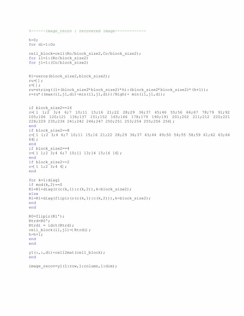
1.1.4 The Matlab Program including above three steps for Image recovery in function form

function

image_recov=idct_zigzag(string,diag1,max,min,High,Ro,Co,Do,block_size2,row,column,d

im)

%------image_recov : recovered image-------------

h=0;

for di=1:Do

cell_block=cell(Ro/block_size2,Co/block_size2);

for i1=1:(Ro/block_size2)

for j1=1:(Co/block_size2)

R1=zeros(block_size2,block_size2);

ru=[];

r=[];

ru=string((1+(block_size2*block_size2)*h):(block_size2*block_size2)*(h+1));

r=ru*((max(i1,j1,di)-min(i1,j1,di))/High)+ min(i1,j1,di);

if block_size2==16

c=[1 1;2 3;4 6;7 10;11 15;16 21;22 28;29 36;37 45;46 55;56 66;67 78;79 91;92

105;106 120;121 136;137 151;152 165;166 178;179 190;191 201;202 211;212 220;221

228;229 235;236 241;242 246;247 250;251 253;254 255;256 256];

end

if block_size2==8

c=[1 1;2 3;4 6;7 10;11 15;16 21;22 28;29 36;37 43;44 49;50 54;55 58;59 61;62 63;64

64];

end

if block_size2==4

c=[1 1;2 3;4 6;7 10;11 13;14 15;16 16];

end

if block_size2==2

c=[1 1;2 3;4 4];

end

for k=1:diag1

if mod(k,2)==0

R1=R1+diag(r(c(k,1):c(k,2)),k-block_size2);

else

R1=R1+diag(fliplr(r(c(k,1):c(k,2))),k-block_size2);

end

end

R0=fliplr(R1');

Rtrd=R0';

Rtrdi = idct(Rtrd);

cell_block(i1,j1)={Rtrdi};

h=h+1;

end

end

y1(:,:,di)=cell2mat(cell_block);

end

image_recov=y1(1:row,1:column,1:dim);

1.2 Using Discrete Wavelet Transform

1.2.1 Image compression using Using Discrete Wavelet Transform

Compression is one of the most important applications of wavelets. Like de-noising, the

compression procedure contains three steps:

1) Decomposiyion: Choose a wavelet, choose a level N. Compute the wavelet decomposition

of the signal at level N.

2) Threshold detail coefficients: For each level from 1 to N, a threshold is selected and hard

thresholding is applied to the detail coefficients.

3) Reconstruct: Compute wavelet reconstruction using the original approximation coefficients

of level N and the modified detail coefficients of levels from 1 to N.

Global Thresholding

The compression features of a given wavelet basis are primarily linked to the relative

scarceness of the wavelet domain representation for the signal. The notion behind

compression is based on the concept that the regular signal component can be accurately

approximated using the following elements: a small number of approximation coefficients (at a

suitably chosen level) and some of the detail coefficients.

n = 5; % Decomposition Level

w = 'sym8'; % Near symmetric wavelet

[c l] = wavedec2(x,n,w); % Multilevel 2-D wavelet decomposition.

In this first method, the WDENCMP function performs a compression process from the wavelet

decomposition structure [c,l] of the image.

opt = 'gbl'; % Global threshold

thr = 20; % Threshold

sorh = 'h'; % Hard thresholding

keepapp = 1; % Approximation coefficients cannot be thresholded

[xd,cxd,lxd,perf0,perfl2] = wdencmp(opt,c,l,w,n,thr,sorh,keepapp);

image(x)

title('Original Image')

colormap(map)

figure('Color','white'),image(xd)

title('Compressed Image - Global Threshold = 20')

colormap(map)

wdencmp: WDENCMP De-noising or compression using wavelets. WDENCMP performs a

de-noising or compression process of a signal or an image using wavelets.

[XC,CXC,LXC,PERF0] = WDENCMP('gbl',X,'wname',N,THR,SORH,KEEPAPP)

returns a de-noised or compressed version XC of input signal X (1-D or 2-D) obtained by

wavelet coefficients thresholding using global positive threshold THR. Additional output

arguments [CXC,LXC] are the wavelet decomposition structure of XC, PERF0 is

compression scores in percentages. Wavelet decomposition is performed at level N and

'wname' is a string containing the wavelet name. SORH ('s' or 'h') is for soft or hard

thresholding. If KEEPAPP = 1, approximation coefficients cannot be threshold, otherwise it is

possible.

Matlab Program for wdencmp

function [xc,cxc,lxc,perf0] = wdencmp(o,varargin)

% Get Inputs

w = varargin{indarg};

n = varargin{indarg+1};

thr = varargin{indarg+2};

sorh = varargin{indarg+3};

if (o=='gbl') , keepapp = varargin{indarg+4}; end

% Wavelet decomposition of x

[c,l] = wavedec2(x,n,w);

% Wavelet coefficients thresholding.

if keepapp

% keep approximation.

cxc = c;

if dim == 1, inddet = l(1)+1:length(c);

else, inddet = prod(l(1,:))+1:length(c); end

% threshold detail coefficients.

cxc(inddet) = c(inddet).*(abs(c(inddet)>thr)); % hard thresholding

else

% threshold all coefficients.

cxc = c.*(abs(c)>thr); % hard thresholding

end

lxc = l;

% Wavelet reconstruction of xd.

if dim == 1,xc = waverec(cxc,lxc,w);

else xc = waverec2(cxc,lxc,w);

end

% Compute compression score.

perf0 = 100*(length(find(cxc==0))/length(cxc));

wavedec2 Multilevel 2-D wavelet decomposition

Syntax

[C,S] = wavedec2(X,N,'wname')

[C,S] = wavedec2(X,N,Lo_D,Hi_D)

Description: wavedec2 is a two-dimensional wavelet analysis function.

[C,S] = wavedec2(X,N,'wname') returns the wavelet decomposition of the matrix X at level N,

using the wavelet named in string 'wname' (see wfilters for more information).

Outputs are the decomposition vector C and the corresponding bookkeeping matrix S.

N must be a strictly positive integer (see wmaxlev for more information).

Instead of giving the wavelet name, you can give the filters.

For [C,S] = wavedec2(X,N,Lo_D,Hi_D), Lo_D is the decomposition low-pass filter and Hi_D is

the decomposition high-pass filter.

Vector C is organized as

C = [ A(N) | H(N) | V(N) | D(N) | ...

H(N-1) | V(N-1) | D(N-1) | ... | H(1) | V(1) | D(1) ].

where A, H, V, D, are row vectors such that

A = approximation coefficients, H = horizontal detail coefficients,

V = vertical detail coefficients, D = diagonal detail coefficients

Each vector is the vector column-wise storage of a matrix.

Matrix S is such that:

S(1,:) = size of app. coef.(N)

S(i,:) = size of det. coef.(N-i+2) for i = 2,...,N+1

and S(N+2,:) = size(X).

Matlab Program for wavedec2

function [c,s] = wavedec2(x,n,IN3)

% [C,S] = WAVEDEC2(X,N,'wname') returns the wavelet

% decomposition of the matrix X at level N, using the wavelet named in string 'wname' (see WFILTERS).

% Outputs are the decomposition vector C and the corresponding bookkeeping matrix S.

s = [size(x)];

c = [];

for i=1:n

[x,h,v,d] = dwt2(x,Lo_D,Hi_D); % decomposition

c = [h(:)' v(:)' d(:)' c]; % store details

s = [size(x);s]; % store size

end

% Last approximation.

c = [x(:)' c];

s = [size(x);s];

DWT2 Single-level discrete 2-D wavelet transform

Syntax

[cA,cH,cV,cD] = dwt2(X,'wname')

[cA,cH,cV,cD] = dwt2(X,Lo_D,Hi_D)

Description

The dwt2 command performs a single-level two-dimensional wavelet decomposition with

respect to either a particular wavelet ('wname', see wfilters for more information) or particular

wavelet decomposition filters (Lo_D and Hi_D) you specify.

[cA,cH,cV,cD] = dwt2(X,'wname') computes the approximation coefficients matrix cA and

details coefficients matrices cH, cV, and cD (horizontal, vertical, and diagonal, respectively),

obtained by wavelet decomposition of the input matrix X. The 'wname' string contains the

wavelet name.

[cA,cH,cV,cD] = dwt2(X,Lo_D,Hi_D) computes the two-dimensional wavelet decomposition

as above, based on wavelet decomposition filters that you specify.

Lo_D is the decomposition low-pass filter.

Hi_D is the decomposition high-pass filter.

Lo_D and Hi_D must be the same length.

Algorithm

For images, there exist an algorithm similar to the one-dimensional case for two-dimensional

wavelets and scaling functions obtained from one- dimensional ones by tensorial product.

This kind of two-dimensional DWT leads to a decomposition of approximation coefficients at

level j in four components: the approximation at level j + 1, and the details in three orientations

(horizontal, vertical, and diagonal).

The following diagram describes the basic decomposition steps for images:

FIGURE 3

TWO-DIMENSIONAL DWT

1.2.2 Matlab Program for Image Compression Using DWT

close all;

clear all;

clc;

X=imread('C:\Documents and Settings\Shrikant Vaishnav\My Documents\My Pictures\My Pictures\lena_dct.bmp');

x=rgb2gray(X);

img=x;

figure(3)

imshow(x)

map=colormap;

figure(1)

image(x)

title('Original Image')

colormap(map)

n = 5; % Decomposition Level

w = 'sym8'; % Near symmetric wavelet

[Lo_D,Hi_D] = wfilters(w,'d');

% Initialization.

a=x;

l = [size(a)];

c = [];

for i=1:n

[a,h,v,d] = dwt2(a,Lo_D,Hi_D); % decomposition........a is approximation Matrix

c = [h(:)' v(:)' d(:)' c]; % store details

l = [size(a);l]; % store size

end

% Last approximation.

c = [a(:)' c];

l = [size(a);l];

% In this first method, the WDENCMP function performs a compression process

% from the wavelet decomposition structure [c,l] of the image.

thr = 50; % Threshold

keepapp = 1; % Approximation coefficients cannot be thresholded

% [cxd,perf0] = compress_dwt(c,l,thr,keepapp);

if keepapp

% keep approximation.

cxd = c;

inddet = prod(l(1,:))+1:length(c);

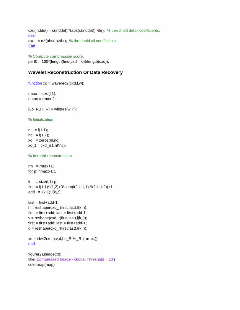
cxd(inddet) = c(inddet).*(abs(c(inddet))>thr); % threshold detail coefficients.

else

cxd = c.*(abs(c)>thr); % threshold all coefficients.

End

% Compute compression score.

perf0 = 100*(length(find(cxd==0))/length(cxd));

Wavelet Reconstruction Or Data Recovery

function xd = waverec2(cxd,l,w);

rmax = size(l,1);

nmax = rmax-2;

[Lo_R,Hi_R] = wfilters(w,'r');

% Initialization.

nl = l(1,1);

nc = l(1,2);

xd = zeros(nl,nc);

xd(:) = cxd_r(1:nl*nc);

% Iterated reconstruction.

rm = rmax+1;

for p=nmax:-1:1

k = size(l,1)-p;

first = l(1,1)*l(1,2)+3*sum(l(2:k-1,1).*l(2:k-1,2))+1;

add = l(k,1)*l(k,2);

last = first+add-1;

h = reshape(cxd_r(first:last),l(k,:));

first = first+add; last = first+add-1;

v = reshape(cxd_r(first:last),l(k,:));

first = first+add; last = first+add-1;

d = reshape(cxd_r(first:last),l(k,:));

xd = idwt2(xd,h,v,d,Lo_R,Hi_R,l(rm-p,:));

end

figure(2),image(xd)

title('Compressed Image - Global Threshold = 20')

colormap(map)

OUTPUT:

dwt_compression_score_in_percentage = perf0 % Compression score

dwt_compression_ratio=100/(100-perf0) % Compression ratio

CHAPTER: 02

INTRODUCTION TO LOSSLESS DATA

COMPRESSION

CHAPTER 02

Introduction to Lossless data Compression

Information Theory & Source Coding

The most significant feature of the communication system is its unpredictability or uncertainty. The

transmitter transmits at random any one of the pre-specified messages. The probability of transmitting

each individual message is known. Thus our quest for an amount of information is virtually a search for

a parameter associated with a probability scheme. The parameter should indicate a relative measure

of uncertainty relevant to the occurrence of each message in the message ensemble.

The principle of improbability (which is one of the basic principles of the media world)--“if a dog bites a

man, it’s no news, but if a man bites a dog, it’s a news”—helps us in this regard. Hence

there should be some sort of inverse relationship between the probability of an event and the amount

of information associated with it. The more the probability of an event, the less is the amount of

information associated with it, & vice versa. Thus,

I(xj)=f(1/p(Xj)), where Xj is an event with a probability p(Xj) & the amount of information associated

with it is I(xj).

Now let there be another event Yk such that Xj & Yk are independent . Hence probability of the

joint event is p(Xj, Yk)= p(Xj) p(Yk) with associated information content ,

I(Xj, Yk)=f(1/p(Xj, Yk))= f(1/p(Xj) (Yk))

The total information I(Xj, Yk) must be equal to the sum of individual information I(Xj) & I(Yk), where

I(Yk)=f(1/p(Yk)). Thus it can be seen that function f must be a function which converts the operation

of multiplication into addition.

LOGARITHM is one such function.

Thus, the basic equation defining the amount of information (or self-information) is,

I(Xj) = log(1/P(Xi)= - log(P(Xi) ,

when base is 2 (or not mentioned)the unit is bit, when base is e the unit is nat, when base is 10 the unit is decit or Hertley.

ENTROPY: Entropy is defined as the average information per individual message.

Let there be L different messages m1, m2…….mL, with their respective probabilities of occurrences be

p1, p2…….pL. Let us assume that in a long time interval, M messages have been generated. Let M be

very large so that M>>L The total amount of information in all M messages.

The number of messages m1=M*p1, the amount of information in message m1= log2(1/P(Xi)), & thus

the total amount of information in all m1 messages = M*p1* log2(1/P(Xi)).

So, the total amount of information in all L messages will then be

I= M*(P1)*log(1/P1)+ M*(P2)*log(1/P2) +………+ M*(PL)*log(1/PL);

So, the average information per message, or entropy, will then be

H=I/M=(P1)*log(1/P1)+ (P2)*log(1/P2) + ………+ (PL)*log(1/PL);

Hence, H(X) = -∑P(Xi) log2(P(Xi)) , summation i=1 to L

The Entropy of a source in bits/symbol is given by

H(X) = -∑P(Xi) log2(P(Xi)) ≤ log2L , summation i=1 to L

Where Xi are the symbols with probabilities P(Xi) , i=1,2,3………..L

The equality holds when the symbols are equally likely.

There are two types of code possible:

1) Fixed Length Code : All code words are of equal length

2) Variable Length Code: All code words are not of equal length. In such cases, it is important for the

formation of uniquely decodable code that all the code words satisfy the PREFIX CCONDITION,

which states that “no code word forms the prefix of any other code word”.

The necessary & sufficient condition for the existence of a binary code with code words having lengths

n1≤n2≤……………nL that satisfy the prefix condition is,

∑ 2^(-nk) ≤ 1 , summation k = 1…………..L ,

which is known as KRAFT INEQUALITY

SOURCE CODING THEORAM:

Let X be ensemble of letters from a discrete memory less source with finite Entropy H(X) & output

symbols Xi with probabilities P(Xi) , i=1,2,3………..L

It is possible to construct a code that satisfies the prefix condition & has an average length R that

satisfies the following inequality,

H(x) ≤ R < H(x)+1,

& the efficiency of the prefix code is defined as η= H(x)/R,

where, H(X) = -∑P(Xi) log2(P(Xi)) , summation i=1 to L

& R = -∑ni log2(P(Xi)) , summation i=1 to L

Here ni denotes the length of ith code word

The source coding theorem tells us that for any prefix code used to represent the symbols from a

source, the minimum number of bits required to represent the source symbols on an average must be

at least equal to the entropy of the source. If we have found a prefix code that satisfies R=H(x) for a

certain source X, we must abandon further search because we can not do any better. The theorem also

tells us that a source with higher entropy (uncertainty) requires on an average, more number of bits to

represent the source symbols in terms of a prefix code.

PROOF:

lower bound:

First consider the lower bound of the inequality. For codewords that have length nk , 1≤k≤L, the

difference H(x)-R can be expressed as

H(x)-R = ∑P(Xk) log2(1/P(Xk)) - ∑P(Xk) nk , summation K=1…………..L

H(x)-R = ∑P(Xk) log2(2^(- nk)/P(Xk)) , summation k=1……………L

H(x)-R ≤ (log2e) ∑P(Xk) { (2^(- nk)/P(Xk))-1} , summation k=1……L

H(x)-R ≤ (log2e) ∑ { (2^(- nk) } – 1 , summation k=1……..…L

H(x)-R ≤ 0 (using KRAFT’S INEQUALITY)

H(x) ≤ R

Upper bound:

Let us select a code word length nk such that

2^(- nk) ≤ P(Xk) < 2^(- nk + 1)

First consider, 2^(- nk) ≤ P(Xk)

∑ 2^(-nk) ≤ ∑ P(Xk) = 1 , summation k=1………….L

Which is the Kraft’s inequality for which there exist a code satisfying the prefix condition

Next consider, P(Xk) < 2^(- nk + 1)

log2(P(Xk)) < (- nk + 1)

nk < 1 - log2(P(Xk))

Multiply both sides by P(Xk)

∑ P(Xk) nk < ∑ P(Xk) + ∑ P(Xk) log2(P(Xk)) , summation k=1……..L

R < H(x)+1

2.2 HUFFMAN CODING

2.2.1 Huffman Coding Algorithm

Huffman coding is an efficient source coding algorithm for source symbols that are not equally

probable. A variable length encoding algorithm was suggested by Huffman in 1952, based on

the source symbol probabilities P(xi), i=1,2…….,L . The algorithm is optimal in the sense that

the average number of bits required to represent the source symbols is a minimum provided

the prefix condition is met. The steps of Huffman coding algorithm are given below:

1. Arrange the source symbols in increasing order of heir probabilities.

2. Take the bottom two symbols & tie them together as shown in Figure 3. Add the

probabilities of the two symbols & write it on the combined node. Label the two branches

with a „1‟ & a „0‟ as depicted in Figure 3

3. Treat this sum of probabilities as a new probability associated with a new symbol. Again

pick the two smallest probabilities, tie them together to form a new probability. Each time

we perform the combination of two symbols we reduce the total number of symbols by one.

Whenever we tie together two probabilities (nodes) we label the two branches with a „0‟ & a

„1‟.

4. Continue the procedure until only one procedure is left (& it should be one if your addition is

correct). This completes the construction of the Huffman Tree.

5. To find out the prefix codeword for any symbol, follow the branches from the final node

back to the symbol. While tracing back the route read out the labels on the branches. This

is the codeword for the symbol.

The algorithm can be easily understood using the following example :

TABLE 1

Symbol Probability Codeword Code length

X1 0.46 1 1

X2 0.30 00 2

X3 0.12 010 3

X4 0.06 0110 4

X5 0.03 01110 5

X6 0.02 011110 6

X7 0.01 011111 6

FIGURE: 4

Huffman Coding for Table 1

The Entropy of the source is found to be

H(X) = -∑P(Xi) log2(P(Xi)) , summation i=1 to 7

H(X) = 1.9781

& R = -∑ni log2(P(Xi)) , summation i=1 to 7

R = 1(0.46)+2(0.30)+3(0.12)+4(0.06)+5(0.03)+6(0.02)+6(0.01)

R = 1.9900

Efficiency, η= H(x)/R = (1.9781/1.9900)= 0.9944

Had the source symbol probabilities been

2^(-1), 2^(-2), 2^(-3), 2^(-4), 2^(-5), 2^(-6), 2^(-6) respectively

then , R=H(x) which gives Efficiency η=1

Huffman Coding for Table 1

2.2.2 MATLAB Program for Huffman Coding in the form of function named “huffman_compression”

function [im_compressed data_length str_code data] = huffman_compression

(signal,Probability,Ro,Co,Do,High1)

%---------huffman_compression-----is the name of function------------

%--------variables---------------

%------signal: input sequence whose Huffman coding is to be done-------

%------im_compressed : output Huffman's coded data sequence(binary)----

lp=length(Probability);

py=round(1000000*Probability);

pyo=zeros(1,lp);

pyo=(py);

pr=fliplr(sort((pyo)));

bit=zeros(1,length(pr));

for ar=1:High1+1

if pr(ar)==0;

data_length=ar-1;

break;

else data_length=ar;

end

end

pr1=zeros(1,data_length);

for j=1:data_length

pr1(j)=pr(j);

end

a=data_length;

d=ones(a,a);

for h=1:a

d(h,1)=h;

end

for e=1:a

t=[];

ph=zeros(a,a);

for n=1:length(pr1)

ph(n,:)=pr1(n);

end

i=0;

for x=2:a

y=ph((length(pr1)-i),x-1)+ ph((length(pr1)-i-1),x-1);

g=0;

for j=1:a

if(g~=1)

if((d(e,x-1)==(length(pr1)-i))||(d(e,x-1)==(length(pr1)-i-1)))

if (y<=(ph(j,x-1)))

ph(j,x)= ph(j,x-1);

else

ph(j,x)=y;

d(e,x)=j;

for k=(j+1):(a-1)

ph(k,x)=ph(k-1,x-1);

end

g=1;

end

else

if (y<=ph(d(e,x-1),x-1));

d(e,x)=d(e,x-1);

else

d(e,x)=d(e,x-1)+1;

end

if (y<=(ph(j,x-1)))

ph(j,x)= ph(j,x-1);

else

ph(j,x)=y;

for k=(j+1):(a-1)

ph(k,x)=ph(k-1,x-1);

end

g=1;

end

end

end

end

i=i+1;

end

end

d;

bit=5*ones(a,a-1);

for x=1:a

j=0;

for i=1:a-1

j=j+1;

if (d(x,i)-(a+1-j))==0

bit(x,i)=0;

else

if (d(x,i)-(a+1-j))==(-1)

bit(x,i)=1;

end

end

end

bit(x,:)=fliplr(bit(x,:));

end

bit;

str_code=cell(a,1);

for i=1:a

h=1;

dt=[];

for j=1:a-1

if(bit(i,j)==0)

dt(h)=0;

h=h+1;

else

if (bit(i,j)==1)

dt(h)=1;

h=h+1;

end

end

end

dt;

str_code(i)=({dt}); %notice { } sign, for conversion to cell type,

end

ph;

xm=[];

for i=1:High1+1

u=0;

for j=0:(High1)

if (round(1000000*Probability(j+1))==round(pr(i)))

len(j+1)=round(Ro*Co*pr(i)/1000000);

u=u+len(j+1);

if(length(find(xm==j))==0)

xm=[xm j];

end

end

end

i=i+u;

end

data=zeros(1,data_length);

for j=1:data_length

data(j)=xm(j);

end

lcomp=0;

tra=signal;

compr=zeros(1,2000000);

for f=1:Ro*Co*Do

for g=1:data_length

if (data(g)==tra(f))

lstrg=length(cell2mat(str_code(g)));

compr(lcomp+1:lcomp+lstrg)=cell2mat(str_code(g));

lcomp=lcomp+lstrg;

forming_compressed_string = lcomp

break

end

end

end

im_compressed=compr(1:lcomp);

2.2.3 HUFFMAN DECODING

The Huffman Code in Table 1 & FIGURE 4 is an instantaneous uniquely decodable block

code. It is a block code because each source symbol is mapped into a fixed sequence of code

symbols. It is instantaneous because each codeword in a string of code symbols can be

decoded without referencing succeeding symbols. That is, in any given Huffman code, no

codeword is a prefix of any other codeword. And it is uniquely decodable because a string of

code symbols can be decoded only in one way. Thus any string of Huffman encoded symbols

can be decoded by examining the individual symbols of the string in left to right manner.

Because we are using an instantaneous uniquely decodable block code, there is no need to

insert delimiters between the encoded pixels.

For Example consider a 19 bit string 1010000111011011111 which can be decoded uniquely

as x1 x3 x2 x4 x1 x1 x7.

A left to right scan of the resulting string reveals that the first valid code word is 1 which is a

code symbol for, next valid code is 010 which corresponds to x1, continuing in this manner, we

obtain a completely decoded sequence given by x1 x3 x2 x4 x1 x1 x7.

2.2.4 MATLAB Program for Huffman Decoding in the function form:

Function recov = recover_data (string1, data_length1, compressed1, padding1,

data1,length_quant1)

%---------variables----------------

% string1 : set of all different codes corresponding to different probability

% data1 : all symbols whose codes are given

% recov : recovered symbols in the sequence that were transmitted after dct &

quantization

le=[1]; % number of discrete codes

k=2;

for x=1:data_length1

ck=1;

w=length(cell2mat(string1(x)));

for jj=1:length(le)

if(le(jj)==w)

ck=0;

end

end

if (ck==1)

le=[le w];

k=k+1;

end

end

if padding1==0

truncate=0

else

truncate=40-padding1;

end

str=0;

reci=1;

recov=zeros(1,length_quant1);

while(str<(length(compressed1)-truncate)) % notice :- '-40+pdg' to compensate

padding

[number position] = recover_num (str, string1, compressed1, data1, le,

data_length1); % le is number of discrete codes

% calling a function which recovers single symbol at a time, one after the other

recov(reci)=number;

str=position;

reci=reci+1;

end

Recovering_compressed_string = 0

recov;

function

[number position]=recover_num(st1,stri,compressed2,data2,le2,data_length2)

%--------"number" is the one recovered symbol with its last bit's "position"---

number=[];

if compressed2(st1+1)==cell2mat(stri(1))

number=data2(1);

position=st1+length(cell2mat(stri(1)));

Recovering_compressed_string = length(compressed2)-position + 1

return

else

for c=2:length(le2)

v=compressed2((1+st1):(le2(c)+st1));

for h=1:data_length2

if(length(cell2mat(stri(h)))==length(v))

if(cell2mat(stri(h))==v)

number=data2(h);

position=st1+length(cell2mat(stri(h)));

Recovering_compressed_string = length(compressed2)-position + 1

return

end

end

end

if(c==length(le2))

error('Data too much corrupted to be decoded')

end

end

end

2.3 SHANNON CODING

2.3.1 SHANNON CODING Algorithm

Shannon coding is yet another coding algorithm, which follows PREFIX Condition & can

achieve compression performance close to that of Huffman coding.

Following are the steps to obtain the codewords by using Shannon Coding Algorithm:

1. Arrange the symbols along with their Probability in decreasing order of Probabilities.

2. Select all those symbols on one side whose probabilities is closest to half of the sum of probabilities of all symbols, & remaining symbols on the other side & assign the values 0 & 1 (first bit of their codeword) respectively to all the symbols in each of the two groups.

3. Select the group having 0 assigned to each of its symbol in step 2 & repeat step 2 for this group. Repeat the same task for the other group (whose symbols have been assigned 1 in the step 2)

4. Repeat step 3 till a group remains to exist like above having more than one symbol.

Diagram(Figure 5) & Table (Table2) in Next Page clearly elaborates the above steps:

FIGURE 5

TABLE 2

Symbol Probability Codeword Code length

X1 0.46 1 1

X2 0.30 01 2

X3 0.12 001 3

X4 0.06 0001 4

X5 0.03 00001 5

X6 0.02 000001 6

X7 0.01 000000 6

The Entropy of the source is found to be

H(X) = -∑P(Xi) log2(P(Xi)) , summation i=1 to 7

H(X) = 1.9781

& R = -∑ni log2(P(Xi)) , summation i=1 to 7

R = 1(0.46)+2(0.30)+3(0.12)+4(0.06)+5(0.03)+6(0.02)+6(0.01)

R = 1.9900

Efficiency, η= H(x)/R = (1.9781/1.9900)= 0.9944

2.3.2 MATLAB program for Shannon coding in the function form:

function [sf_code data_length str_code

data]=sha_fan(signal,Probability,High1)

lp=length(Probability);

pyo=Probability;

pr=fliplr(sort((pyo)));

for ar=1:High1+1

if pr(ar)==0;

data_length=ar-1;

break;

else data_length=ar;

end

end

pr1=zeros(1,data_length);

for j=1:data_length

pr1(j)=pr(j);

end

data_length;

pr1;

code=5*ones(length(pr1),length(pr1)+1);

t=[1 data_length+1];

temp=[];

i=1;

while((length(t)-1)<length(pr1))

if i+1>length(t)

i=1;

end

diff(i)=t(i+1)-t(i)-1;

if diff(i)>0

ss=sum(pr1(t(i):(t(i+1)-1)))/2 ;

for k=t(i):(t(i+1)-1)

if (sum(pr1(t(i):k))<(ss))

else

k;

h=1;

for r=(t(i)):k

while((code(r,h)==0)||(code(r,h)==1))

h=h+1;

end

code(r,h)=0;

end

for rr=k+1:(t(i+1)-1)

code(rr,h)=1;

end

temp=k+1;

break;

end

end

t=[t temp];

t=sort(t);

end

i=i+1;

end

a=length(pr1);

str_code=cell(a,1);

for i=1:a

h=1;

dt=[];

for j=1:a

if(code(i,j)==0)

dt(h)=0;

h=h+1;

else

if (code(i,j)==1)

dt(h)=1;

h=h+1;

end

end

end

dt;

str_code(i)=({dt});

end

xm=[];

for i=1:High1+1

u=0;

for j=0:(High1)

if ((Probability(j+1))==(pr(i)))

len(j+1)=round(length(signal)*pr(i));

u=u+len(j+1);

if(length(find(xm==j))==0)

xm=[xm j];

end

end

end

i=i+u;

end

data=zeros(1,data_length);

for j=1:data_length

data(j)=xm(j);

end

lcomp=0;

tra=signal;

compr=zeros(1,2000000);

for f=1:length(tra)

for g=1:data_length

if (data(g)==tra(f))

lstrg=length(cell2mat(str_code(g)));

compr(lcomp+1:lcomp+lstrg)=cell2mat(str_code(g));

lcomp=lcomp+lstrg;

forming_compressed_string = lcomp

break

end

end

end

sf_code=compr(1:lcomp);

2.3.3 Decoding Process for Shannon Code The Decoding Process of Shannon Codes is identical to that of Huffman Codes as it also

satisfies Prefix Condition & forms uniquely decodable code.

2.3.4 MATLAB Program for Shannon Decoding in the function form:

function recov = recover_data_sh

(string1,data_length1,compressed1,padding1,data1,length_quant1)

%---------variables---------------- % string1 : set of all different codes corresponding to different probability

% data1 : all symbols whose codes are given % recov : recovered symbols in the sequence that were transmitted after dct

& quantization

data1; le=[1]; % number of discrete codes k=2;

for x=1:data_length1 ck=1; w=length(cell2mat(string1(x))); for jj=1:length(le) if(le(jj)==w) ck=0; end end if (ck==1) le=[le w]; k=k+1; end

end

if padding1==0 truncate=0; else truncate=40-padding1; end

str=0; reci=1; recov=zeros(1,length_quant1); while(str<(length(compressed1)-truncate)) % notice :- '-40+pdg' to compensate

padding [number position]

=recover_num_sh(str,string1,compressed1,data1,le,data_length1);

% le is number of discrete codes % calling a function which recovers single symbol at a time, one after the

other

recov(reci)=number; str=position; reci=reci+1; end Recovering_compressed_string = 0

recov; function [number position] =

recover_num_sh(st1,stri,compressed2,data2,le2,data_length2)

%--------"number" is the one recovered symbol with its last bit's "position"-

--

number=[];

for c=1:length(le2) v=compressed2((1+st1):(le2(c)+st1)); for h=1:data_length2 if(length(cell2mat(stri(h)))==length(v)) if(cell2mat(stri(h))==v) v; number=data2(h); position=st1+length(cell2mat(stri(h))); Recovering_compressed_string = length(compressed2)-position +

1 return end end end

if(c==length(le2)) error('Data too much corrupted to be decoded') end end

PART: II

TRANSMISSION

THROUGH

DIGITAL COMMUNICATION CHANNEL

CHAPTER: 01

CHANNEL CODING

CHAPTER 01

CHANNEL CODING

All real life channels are affected by noise. Noise causes discrepancies (errors) between the

input & the output data sequences of a digital communication system. In order to achieve

reliability we have to resort to the use of channel coding. The basic objective of channel coding

is to increase the resistance of the digital communication system to channel noise. This is

done by adding redundancies in the transmitted data stream in a controlled manner. In channel

coding we map the incoming data sequence to a channel input sequence. This encoding

procedure is done by the channel encoder. The encoded sequence is then transmitted over

the noisy channel. The channel output sequence at the receiver is inversely mapped to an

output data sequence. This is called the decoding procedure, and is carried out by the

channel decoder.

Channel coding is also referred to as Error Control Coding. It is interesting to note here that the

source coder reduces redundancy to improve efficiency, where as the channel coder adds

redundancy, in a controlled manner, to improve reliability.

1.1 BLOCK CODING & HAMMING CODES

Consider a message source can generate M equally likely messages. Then initially we

represent each message by k binary digits with 2^k=M. These k bits are the information

bearing bits. We next add to each k bit message, r redundant bits (parity check bits). Thus

each message has been expanded into a codeword of length n bits with n=k+r. The total

number of possible n bit codeword is 2^n while the total number of possible messages is 2^k.

There are therefore 2^n - 2^k possible n bit words which do not represent possible messages.

Codes formed by taking a block of k information bits & adding r (= n-k) redundant bits to form a

codeword are called block codes & designated as (n,k) codes.

ENCODING:

The generation of a block code starts with a selection of the number r of parity bits to be added

& thereafter with the specification of H matrix known as Parity Check Matrix.

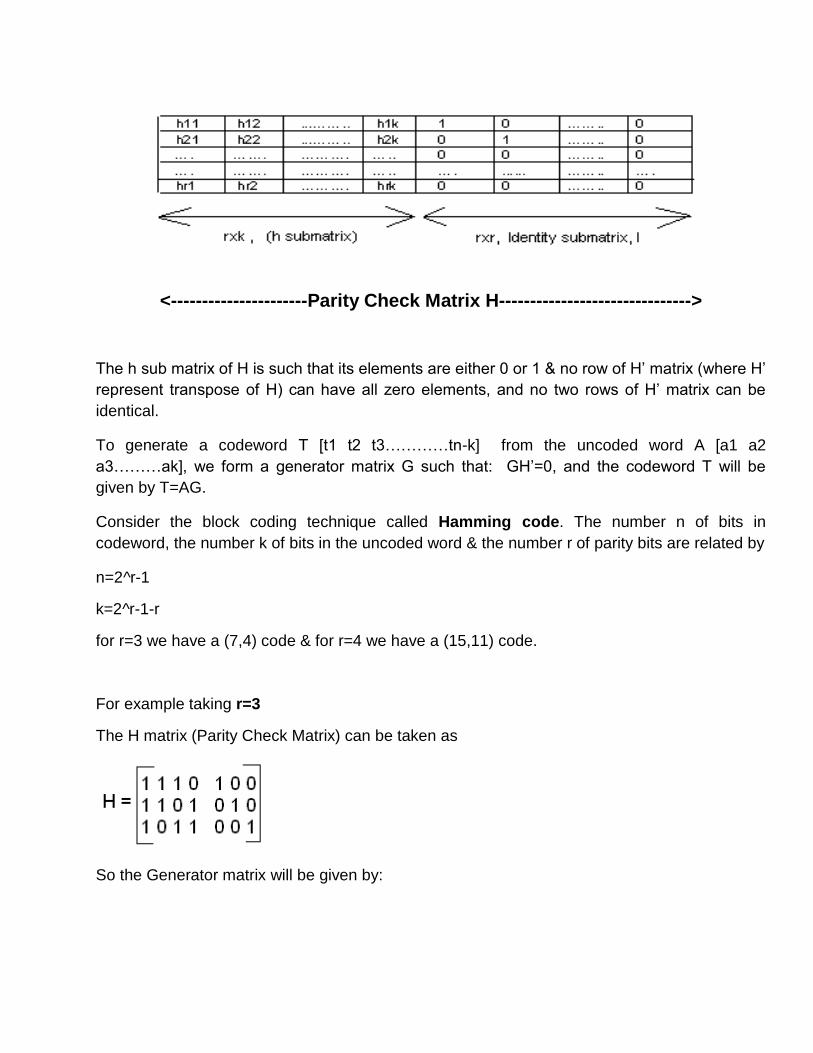
<----------------------Parity Check Matrix H------------------------------->

The h sub matrix of H is such that its elements are either 0 or 1 & no row of H‟ matrix (where H‟

represent transpose of H) can have all zero elements, and no two rows of H‟ matrix can be

identical.

To generate a codeword T [t1 t2 t3…………tn-k] from the uncoded word A [a1 a2

a3………ak], we form a generator matrix G such that: GH‟=0, and the codeword T will be

given by T=AG.

Consider the block coding technique called Hamming code. The number n of bits in

codeword, the number k of bits in the uncoded word & the number r of parity bits are related by

n=2^r-1

k=2^r-1-r

for r=3 we have a (7,4) code & for r=4 we have a (15,11) code.

For example taking r=3

The H matrix (Parity Check Matrix) can be taken as

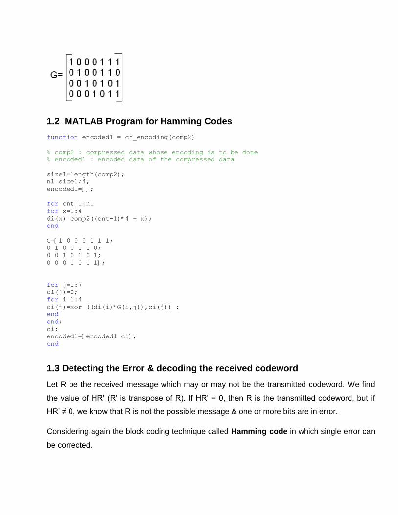
So the Generator matrix will be given by:

1.2 MATLAB Program for Hamming Codes

function encoded1 = ch_encoding(comp2)

% comp2 : compressed data whose encoding is to be done

% encoded1 : encoded data of the compressed data

size1=length(comp2);

n1=size1/4;

encoded1=[];

for cnt=1:n1

for x=1:4

di(x)=comp2((cnt-1)*4 + x);

end

G=[1 0 0 0 1 1 1;

0 1 0 0 1 1 0;

0 0 1 0 1 0 1;

0 0 0 1 0 1 1];

for j=1:7

ci(j)=0;

for i=1:4

ci(j)=xor ((di(i)*G(i,j)),ci(j)) ;

end

end;

ci;

encoded1=[encoded1 ci];

end

1.3 Detecting the Error & decoding the received codeword

Let R be the received message which may or may not be the transmitted codeword. We find

the value of HR‟ (R‟ is transpose of R). If HR‟ = 0, then R is the transmitted codeword, but if

HR‟ ≠ 0, we know that R is not the possible message & one or more bits are in error.

Considering again the block coding technique called Hamming code in which single error can

be corrected.

For r=3 & H matrix (Parity Check Matrix) again taken as

Then for R= [1 0 0 0 0 1 1]

Let the syndrome vector be S=HR‟

Clearly S is obtained to be S = [1 0 0]

Comparing S with H’ (transpose of H) we find that 5th row from top of H’ is same as S as shown below:

So vector R also has the error in 5th bit from left i.e the transmitted codeword was T=[1 0 0 0 1

1 1]. Hence the error is detected & received code word is correctly decoded by extracting the

1st k (=4) information bit from T which is given by A=[1 0 0 0].

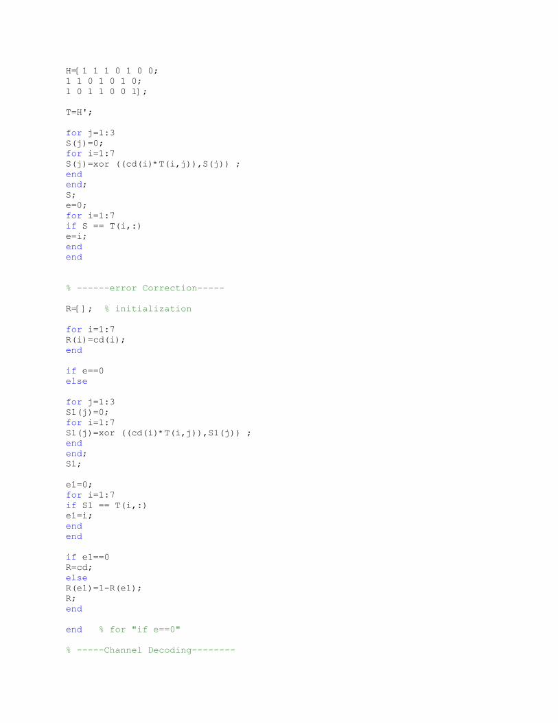
1.4 MATLAB Program for Error Detection & Channel Decoding in Function form

function decoded1=ch_decoding(demodulated2)

%---------demodulated2 : demodulated data whose decoding is to be done--

%---------decoded1 : obtained decoded data---------

decoded1=[];

size5=length(demodulated2);

n5=round(size5/7);

for cnt=1:n5

for x=1:7

cd(x)=demodulated2((cnt-1)*7 + x);

end

% ----test for ERROR---

H=[1 1 1 0 1 0 0;

1 1 0 1 0 1 0;

1 0 1 1 0 0 1];

T=H';

for j=1:3

S(j)=0;

for i=1:7

S(j)=xor ((cd(i)*T(i,j)),S(j)) ;

end

end;

S;

e=0;

for i=1:7

if S == T(i,:)

e=i;

end

end

% ------error Correction-----

R=[]; % initialization

for i=1:7

R(i)=cd(i);

end

if e==0

else

for j=1:3

S1(j)=0;

for i=1:7

S1(j)=xor ((cd(i)*T(i,j)),S1(j)) ;

end

end;

S1;

e1=0;

for i=1:7

if S1 == T(i,:)

e1=i;

end

end

if e1==0

R=cd;

else

R(e1)=1-R(e1);

R;

end

end % for "if e==0"

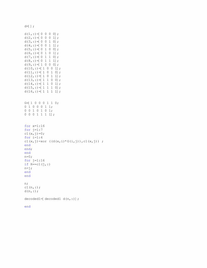
% -----Channel Decoding--------

d=[];

d(1,:)=[0 0 0 0];

d(2,:)=[0 0 0 1];

d(3,:)=[0 0 1 0];

d(4,:)=[0 0 1 1];

d(5,:)=[0 1 0 0];

d(6,:)=[0 1 0 1];

d(7,:)=[0 1 1 0];

d(8,:)=[0 1 1 1];

d(9,:)=[1 0 0 0];

d(10,:)=[1 0 0 1];

d(11,:)=[1 0 1 0];

d(12,:)=[1 0 1 1];

d(13,:)=[1 1 0 0];

d(14,:)=[1 1 0 1];

d(15,:)=[1 1 1 0];

d(16,:)=[1 1 1 1];

G=[1 0 0 0 1 1 0;

0 1 0 0 0 1 1;

0 0 1 0 1 0 1;

0 0 0 1 1 1 1];

for x=1:16

for j=1:7

c1(x,j)=0;

for i=1:4

c1(x,j)=xor ((d(x,i)*G(i,j)),c1(x,j)) ;

end

end;

end

n=0;

for j=1:16

if R==c1(j,:)

n=j;

end

end

n;

c1(n,:);

d(n,:);

decoded1=[decoded1 d(n,:)];

end

CHAPTER: 02

MODULATION

CHAPTER 02

SIGNAL MODULATION

2.1 SIGNAL MODULATION USING BINARY PHASE SHIFT KEYING (BPSK)

In binary phase shift keying (BPSK) the transmitted signal is a sinusoid of fixed amplitude. It

has one fixed phase when the data is at one level & when the data is at the other level the

phase is different by 180 degree. If the sinusoid is of amplitude A. The transmitted signal is

either A*cos(wt) or –A*cos(wt). In BPSK, the data b(t) is a stream of binary digits with voltage

levels which as a matter of convenience, we take to be at +1V or -1V. When b(t)=1V we say it

is at logic level 1 & when b(t) = -1V we say it is at logic level 0. Hence V(bpsk) can be written,

with no loss of generality, as

V(bpsk)=b(t)*Acos(wt)

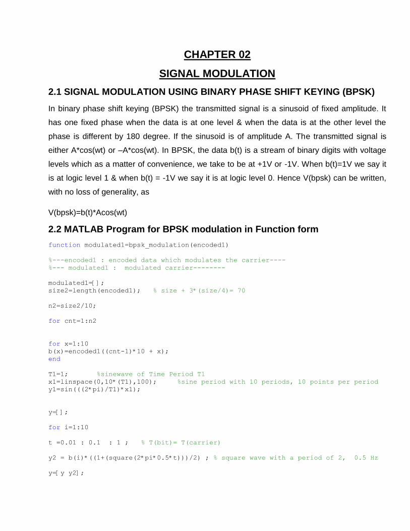
2.2 MATLAB Program for BPSK modulation in Function form

function modulated1=bpsk_modulation(encoded1)

%---encoded1 : encoded data which modulates the carrier----

%--- modulated1 : modulated carrier--------

modulated1=[];

size2=length(encoded1); % size + 3*(size/4)= 70

n2=size2/10;

for cnt=1:n2

for x=1:10

b(x)=encoded1((cnt-1)*10 + x);

end

T1=1; %sinewave of Time Period T1

x1=linspace(0,10*(T1),100); %sine period with 10 periods, 10 points per period

y1=sin(((2*pi)/T1)*x1);

y=[];

for i=1:10

t =0.01 : 0.1 : 1 ; % T(bit)= T(carrier)

y2 = b(i)*((1+(square(2*pi*0.5*t)))/2) ; % square wave with a period of 2, 0.5 Hz

y=[y y2];

end

y=2*(y-(1/2));

t=0.01:0.1:1;

%---------------MODULATION-------------------

t=0.01:0.1:1;

vm=[];

vm=y.*y1;

modulated1=[modulated1 vm];

end

2.3 RECEPTION OF BPSK

The received signal has the form V(bpsk)=b(t)*Acos(wt+$). Here $ is the phase shift

corresponding to the time delay which depends on the length of the path from transmitter to

receiver & the phase shift produced by the amplifiers in the front end of the receiver preceding

the demodulator. The original data b(t) is recovered in the demodulator. The demodulation

technique usually employed is called synchronous demodulation & requires that there be

available at the demodulator the wave form cos(wt + $). A scheme for generating the carrier at

the demodulator & for recovering the baseband signal is shown in Figure 6

FIGURE 6

Scheme to recover the baseband signal in BPSK

The received signal is squared to generate the signal

(Cos(wt+$))^2 = ½(1 + cos(wt+$))

The dc component is removed by the bandpass filter whose passband is centered around 2fo

& we then have the signal whose waveform is that of cos2(wt + $). A frequency divider

(composed of a flip-flop & a narrow band filter tuned at fo) is used to regenerate the wave form

cos(wt+$).Only the waveforms of the signals at the outputs of the squarer, filter & divider are

relevant to our discussion & not their amplitudes. Accordingly in Figure 5, we have arbitrarily

taken each amplitude to be unity. In practice the amplitude will be determined by features of

these devices which are of no present concern. In any event, the carrier having been

recovered, it is multiplied with the received signal to generate

b(t)*A((cos (wt+$))^2) = b(t)*A½(1 + cos(wt+$))

which is then applied to an integrator as shown in Figure 5

We have included in the system a bit synchronizer. This device precisely recognizes the

moment which corresponds to the end of the time interval allocated to one bit and the

beginning of the next. At that moment it closes the switch Sc very briefly to discharge(dump)

the integrator capacitor & leaves the switch Sc open during the entire course of the ensuing bit

interval, closing switch again very briefly at the end of the next bit time. This circuit is called an

integrate & dump circuit.

The output signal of interest to us is the integrator output at the end of a bit interval but

immediately before the closing of switch Sc. The output signal is made available by switch Ss

which samples the output voltage just prior to dumping the capacitor.For simplicity the bit

interval Tb is equal to the duration of an integral number n of cycles of the carrier frequency fo,

that is n.2π=wTb.

In this case the output voltage Vo(kTb) at the end of a bit interval extending from time (k-1)Tb to kTb is :

Vo(kTb) = A*b(kTb)* ∫1/2dt + A*b(kTb)* ∫1/2*cos2(wt+$)dt

= b(kTb)*(A/2)Tb

Since the integral of a sinusoid over a whole number of cycles has the value zero. Thus we

see that our system reproduces at the demodulator output the transmitted bit stream b(t).

2.4 MATLAB Program for BPSK demodulation in Function form

function demodulated1=bpsk_demodulation(equalized2)

%---equalized : equalized data to be demodulated---

%----demodulated1 : demodulated data--------

demodulated1=[];

size4=length(equalized2);

n4=size4/100;

for cnt=1:n4

for x=1:100

v(x)=equalized2((cnt-1)*100 + x);

end

T1=1; %sinewave of Time Period To

x1=linspace(0,10*(T1),100); %sine period with 10 periods, 25 points per period

y1=sin(((2*pi)/T1)*x1);

f=[];

f=v.*y1;

Tb=1;

n=100;

h=Tb/n;

for k=1:10

s1=0;

s2=0;

for i=(10*(k-1))+1 : k*10

if mod(i,3)==0

s1=s1+f(i);

else

s2=s2+f(i)-f(k*10);

end

end

vdm(k*Tb)=3*h/8*(f(k*10)+3*(s2)+2*(s1));

end

vdm=2*vdm;

vdmb=[];

for i=1:10

if vdm(i)<0

vdmb(i)=0;

else

vdmb(i)=1;

end

end

demodulated1=[demodulated1 vdmb];

end

CHAPTER: 03

CHANNEL EQUALIZATION

CHAPTER 03

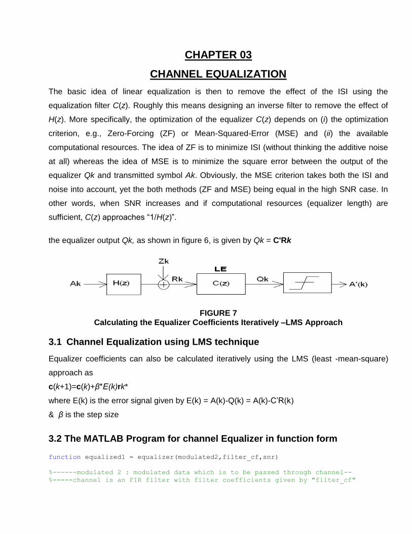
CHANNEL EQUALIZATION

The basic idea of linear equalization is then to remove the effect of the ISI using the

equalization filter C(z). Roughly this means designing an inverse filter to remove the effect of

H(z). More specifically, the optimization of the equalizer C(z) depends on (i) the optimization

criterion, e.g., Zero-Forcing (ZF) or Mean-Squared-Error (MSE) and (ii) the available

computational resources. The idea of ZF is to minimize ISI (without thinking the additive noise

at all) whereas the idea of MSE is to minimize the square error between the output of the

equalizer Qk and transmitted symbol Ak. Obviously, the MSE criterion takes both the ISI and

noise into account, yet the both methods (ZF and MSE) being equal in the high SNR case. In

other words, when SNR increases and if computational resources (equalizer length) are

sufficient, C(z) approaches “1/H(z)”.

the equalizer output Qk, as shown in figure 6, is given by Qk = C'Rk

FIGURE 7 Calculating the Equalizer Coefficients Iteratively –LMS Approach

3.1 Channel Equalization using LMS technique

Equalizer coefficients can also be calculated iteratively using the LMS (least -mean-square)

approach as

c(k+1)=c(k)+β*E(k)rk*

where E(k) is the error signal given by E(k) = A(k)-Q(k) = A(k)-C‟R(k)

& β is the step size

3.2 The MATLAB Program for channel Equalizer in function form function equalized1 = equalizer(modulated2,filter_cf,snr)

%------modulated 2 : modulated data which is to be passed through channel--

%-----channel is an FIR filter with filter coefficients given by "filter_cf"

%-----equalized1 : data after passing through filter & its' equalizer----

equalized1=[];

size3=length(modulated2);

n3=size3/5;

for cnt=1:n3

cnt;

a=[];

rv=[];

for x=1:5

a(x)=modulated2((cnt-1)*5 + x);

end

%------- ADDITION OF NOISE---------

s = cov(a);

n = s/(10^((snr)));

amp = sqrt(n/2);

noise= amp*randn(1,5);

a=a+noise;

for r=1:3

a=[a a];

end

Rk=filter(filter_cf,1,a); % Received Signal

if cnt<10

beta=0.1;% step Size of the algorithm

else

beta=0.25;

end

c=zeros(5,1); % equalizer coefficients

for i=1:length(Rk)-4,

rk=flipud(Rk(i:i+4).'); % received Signal Vector

Error(i)=a(i)-c.'*rk; % Error signal, we assume a known symbol sequence

c=c+beta*Error(i)*rk; % LMS update

end

for i=31:length(Rk)-5,

rk=flipud(Rk(i:i+4).'); % received Signal Vector

Error(i)=a(i)-c.'*rk; % Error signal, we assume a known symbol sequence

rv(i-30)=c.'*rk;

end

equalized1=[equalized1 rv];

end

CHAPTER: 04

Digital Communication System

Implementation

CHAPTER 04

Digital Communication System Implementation

Figure 8

Digital Communication System

4.1 The MATLAB Program to implement the Digital Communication system

clear all;

clc;

close all;

x=imread('D:\My Pictures\s.bmp');

image=double(x)/255;

[Rows Columns Dimensions]=size(image);

figure(1)

imshow(image)

t0=cputime;

%-------Finding The Discrete Cosine Transform------------

%-------finding the transform------------

block_size=input('Size of blocks ');

diagonals=input('Number of diagonals to be considered ZigZag traversing ');

quantization_level=input('Number of quantization_levels ');

[quant_image High max min Ro Co Do]=

dct_zigzag (image,Rows,Columns,Dimensions,diagonals,quantization_level,block_size);

length_quant=length(quant_image);

%-------huffman---encodinig-----------------

%--finding the probability--

Probability=zeros(1,High+1);

for i=0:High

Probability(i+1)=length(find(quant_image==i))/(Ro*Co);

end

[compressed data_length codes data]

= huffman_compression(quant_image,Probability,Ro,Co,Do,High);

%--------Data Transmission------------

%--------channel encoding----Modulation(bpsk)------channel Equalization-----

%--------Demodulation--------channel Decoding-----------------------------

[compressed_padded padding n0]=data_padding(compressed);

%-----Padding the data with sufficient number of bits so that a block of 40

% bits is taken at a time for processing, one after the other --------

% n0 is the total number of such 40 bit blocks formed---------

seconds=0;

comprd=[];

for count=1:n0

In_Enco__BPSK__Ch_Equa = n0-count

seconds=(cputime-t0);

comp1=zeros(1,40);

for x=1:40

comp1(x)=compressed_padded((count-1)*40 + x);

end

% -----------Channel Encoding----------------

[encoded] = ch_encoding(comp1);

% -------------Modulation----------------

modulated=bpsk_modulation(encoded);

%-----------Channel Equalization-------------

filter_coeff=fir1(8,0.6);

snr=4;

equalized=equalizer(modulated,filter_coeff,snr);

% ------------DEMODULATION---------------------

demodulated=bpsk_demodulation(equalized);

% ----------CHANNEL DECODING-------------------

decoded=ch_decoding(demodulated);

comprd=[comprd decoded];

end

compressed_pro=comprd;

% % when channel not used

% compressed_pro=compressed;

% padding=0;

% ----------DATA RECOVERY------OR------HUFFMAN DECODING-------------

recovered_data = recover_data (codes, data_length, compressed_pro, padding, data,

length_quant);

%------------------IMAGE--RECOVERY----------------

%----------------IDCT---&--Zigzag Decoding-------

recovered_image=idct_zigzag(recovered_data,diagonals,max,min,High,Ro,Co,Do,block_si

ze,Rows,Columns,Dimensions);

%---------------------OUTPUT--------------------

figure(4)

imshow(recovered_image);

MSE=sqrt(sum(((recovered_image(:)-image(:)).^2))/(Ro*Co*Do));

SNR=sqrt((sum((recovered_image(:)).^2))/(Ro*Co*Do))/MSE;

RUN_TIME_IN_MINUTES=(cputime-t0)/60

quantization_level

Size_of_Block_taken_for_DCT = block_size

Nmber_of_diagonals = diagonals

COMPRESSION_RATIO = 8*Ro*Co*Do/length(compressed)

SNR

CHAPTER: 05

RESULTS (Observation)

CHAPTTER 05

RESULTS (OBSERVATION)

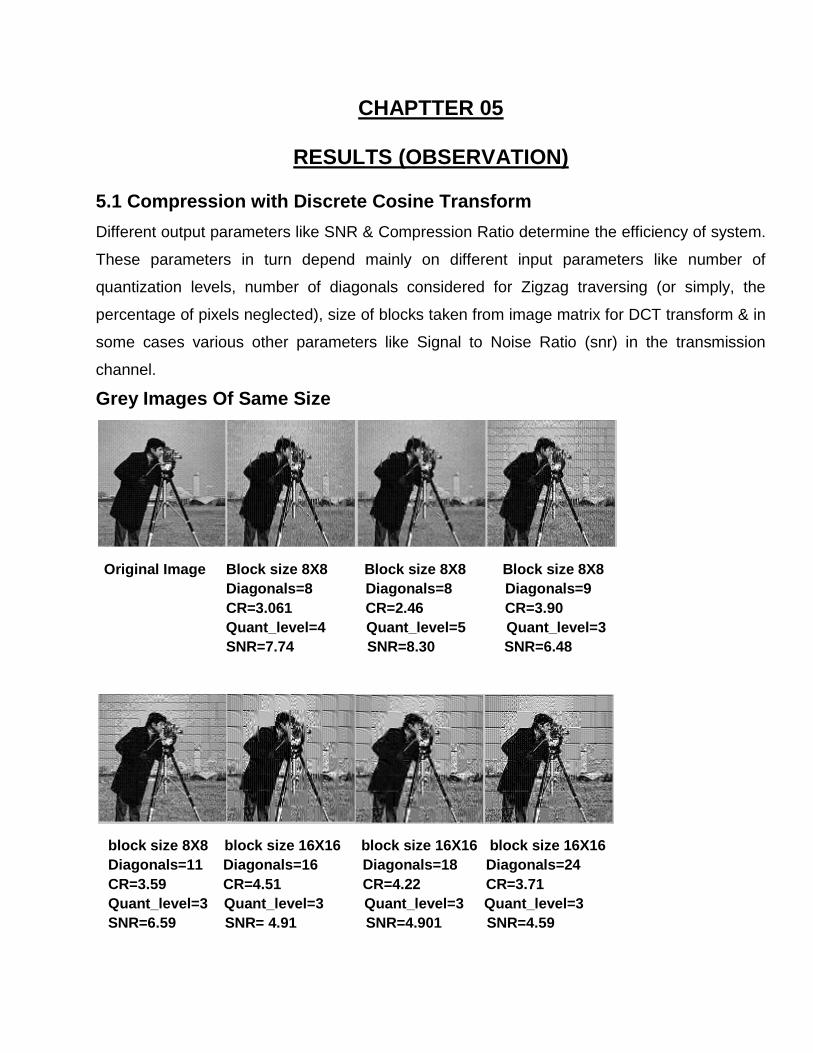
5.1 Compression with Discrete Cosine Transform

Different output parameters like SNR & Compression Ratio determine the efficiency of system.

These parameters in turn depend mainly on different input parameters like number of

quantization levels, number of diagonals considered for Zigzag traversing (or simply, the

percentage of pixels neglected), size of blocks taken from image matrix for DCT transform & in

some cases various other parameters like Signal to Noise Ratio (snr) in the transmission

channel.

Grey Images Of Same Size

Original Image Block size 8X8 Block size 8X8 Block size 8X8

Diagonals=8 Diagonals=8 Diagonals=9

CR=3.061 CR=2.46 CR=3.90

Quant_level=4 Quant_level=5 Quant_level=3

SNR=7.74 SNR=8.30 SNR=6.48

block size 8X8 block size 16X16 block size 16X16 block size 16X16

Diagonals=11 Diagonals=16 Diagonals=18 Diagonals=24

CR=3.59 CR=4.51 CR=4.22 CR=3.71

Quant_level=3 Quant_level=3 Quant_level=3 Quant_level=3

SNR=6.59 SNR= 4.91 SNR=4.901 SNR=4.59

The values of corresponding input & output parameters for different sized gray

images by varying the Block size taken for DCT & number of coefficients

selected for transmission are tabularized as shown. Quantization Level is fixed

for the entire observation.

TABLE 3 Image Size Block Size

taken for DCT Diagonals taken

Quantization Level

SNR (received Image)

Compression Ratio

128x128 4X4 4 3 8.00 3.99

128x128 4X4 5 3 9.27 3.55

128x128 4X4 6 3 10.20 3.36

128x128 8X8 9 3 6.48 3.90

128x128 8X8 10 3 6.59 3.59

128x128 8X8 11 3 6.68 3.33

128x128 16X16 16 3 4.91 4.51

128x128 16X16 18 3 4.91 4.22

128x128 16X16 24 3 4.60 3.71

128x128 16X16 27 3 4.49 3.58

256x256 4X4 4 3 9.01 4.37

256x256 4X4 5 3 10.27 4.21

256x256 4X4 6 3 10.80 4.07

256x256 8X8 9 3 7.61 4.20

256x256 8X8 10 3 7.73 3.66

256x256 8X8 11 3 8.19 3.21

256x256 16X16 16 3 6.01 4.51

256x256 16X16 18 3 6.22 4.21

256x256 16X16 24 3 6.64 3.34

256x256 16X16 27 3 6.81 3.02

The values of corresponding input & output parameters for different sized gray

images by varying the Quantization Level & Block size taken for DCT are

tabularized as shown. Number of Coefficients selected for transmission is kept

fixed for the entire observation.

TABLE 4 Image Size

Block Size taken for DCT

Diagonals taken

Quantization Level


Compression Ratio

128x128 4X4 6 3 8.00 3.99

128x128 4X4 6 4 9.27 3.55

128x128 4X4 6 5 10.20 3.36

128x128 4x4 6 6 11.16 3.27

128x128 8X8 8 4 7.74 4.10

128x128 8X8 8 5 8.30 3.76

128x128 8X8 8 6 9.22 3.19

128x128 8x8 8 7 9.64 3.08

128x128 16X16 11 5 7.46 5.51

128x128 16X16 11 6 7.91 5.64

128x128 16X16 11 7 8.11 5.91

128x128 16X16 11 8 8.54 6.04

256x256 4X4 6 3 8.80 4.91

256x256 4X4 6 4 9.87 4.55

256x256 4X4 6 5 10.96 4.36

256x256 4x4 6 6 11.91 4.17

256x256 8X8 8 4 8.94 5.10

256x256 8X8 8 5 9.30 4.66

256x256 8X8 8 6 9.82 4.39

256x256 8x8 8 7 10.44 4.28

256x256 16X16 11 5 8.46 6.11

256x256 16X16 11 7 9.11 5.81

256x256 16X16 11 8 9.98 5.66

COLOURED IMAGES OF DIFFERENT SIZE Now for coloured image taking 8X8 as the block size for DCT, the SNR & the Compression

Ratio obtained for different number of diagonals taken for some 256X256 Images are as

follows:

256X256 Original Image

Diagonals taken = 5 Diagonals taken = 8 Diagonals taken = 9 SNR = 1.59 SNR = 13.52 SNR = 16.41 Compr. Ratio = 5.62 Compr. Ratio = 3.70 Compr Ratio = 3.27

Where as continuing same technique (8X8 block, 10 diagonals) but for a

512X512 Image yields:

The values of corresponding input & output parameters for different sized

coloured Images by taking fixed Quantization level is tabularized as shown

below:



Quantization Level


Compression Ratio

128x128 4X4 4 3 9.00 4.89

128x128 4X4 5 3 9.87 4.55

128x128 4X4 6 3 11.20 4.36

128x128 8X8 9 3 7.48 4.20

128x128 8X8 10 3 7.79 4.09

128x128 8X8 11 3 8.88 3.93

128x128 16X16 16 3 5.71 5.51

128x128 16X16 18 3 5.90 5.28

128x128 16X16 24 3 6.10 5.11

128x128 16X16 27 3 6.19 4.98

256x256 4X4 4 3 9.51 4.97

256x256 4X4 5 3 10.17 4.61

256x256 4X4 6 3 10.40 4.37

256x256 8X8 9 3 8.41 4.20

256x256 8X8 10 3 8.70 3.66

256x256 8X8 11 3 8.99 3.21

256x256 16X16 16 3 6.71 5.61

256x256 16X16 18 3 6.92 5.34

256x256 16X16 24 3 7.34 4.89

256x256 16X16 27 3 7.71 4.62

The values of corresponding input & output parameters for different sized

coloured images by varying the Quantization Level & Block size taken for DCT

are tabularized as shown. Number of Coefficients selected for transmission is

kept fixed for the entire observation.



Quantization Level


Compression Ratio

128x128 4X4 6 3 9.30 4.96

128x128 4X4 6 4 9.77 4.55

128x128 4X4 6 5 10.90 4.16

128x128 4x4 6 6 11.76 3.97

128x128 8X8 8 4 8.79 5.22

128x128 8X8 8 5 9.30 4.92

128x128 8X8 8 6 9.92 4.67

128x128 8x8 8 7 10.64 4.58

128x128 16X16 11 5 8.79 6.41

128x128 16X16 11 6 9.31 6.30

128x128 16X16 11 7 8.91 6.17

128x128 16X16 11 8 9.54 6.04

256x256 4X4 6 3 9.20 5.79

256x256 4X4 6 4 10.37 5.65

256x256 4X4 6 5 11.16 5.46

256x256 4x4 6 6 12.01 5.27

256x256 8X8 8 4 10.69 5.10

256x256 8X8 8 5 11.34 4.66

256x256 8X8 8 6 11.92 4.39

256x256 8x8 8 7 12.44 4.28

256x256 16X16 11 6 10.51 6.85

256x256 16X16 11 7 10.91 6.51

256x256 16X16 11 8 11.48 6.34

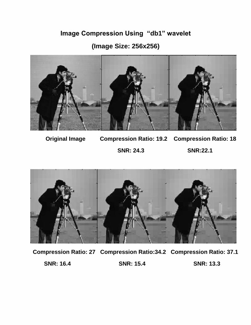
5.2 Compression with Discrete Wavelet Transform

Output parameters like compression score, compression ratio determines the efficiency of

system. These parameters in turn depend mainly on different input parameters like number of

decomposition levels, threshold, size of image matrix etc.

Grey Image Of size 256x256:

Decomposition Level:5 Decomposition Level: 5 Decomposition Level: 5

Threshold: 40 Threshold: 50 Threshold: 65

Original Image Compression_score: 92.5 Compression_score: 93.9 Compressionscore: 95.3

Compression_ratio: 13.29 Compression_ratio: 13.29 Compression_ratio: 13.29

Decomposition Level: 5 Decomposition Level: 5 Decomposition Level: 5

Threshold: 40 Threshold: 50 Threshold: 65

Original Image Compression_score: 91.6 Compression_score: 93.1 Compressionscore: 94.5

Compression_ratio: 11.86 Compression_ratio: 14.48 Compression_ratio: 18.37

It can be observed that for a fixed Decomposition Level, the increase in value of Threshold

results in greater compression. While for a fixed value of Threshold, compression score/ratio

decreases with increase in Decomposition Level. Also better compression results are obtained

for images of larger size. All these observations are also verified by the table shown in next

page.

Image Compression Using “sym4” wavelet

(Image Size: 256x256)

Original Image 22 Compression Ratio: 27 Compression Ratio: 29.1

SNR: 11.4 SNR: 10.3

Compression Ratio: 30.1 Compression Ratio: 34.5 Compression Ratio: 39

SNR: 9.2 SNR: 8.7 SNR:8.1

The values of corresponding input & output parameters using “sym4” wavelet for

various size images are tabularized as shown:

TABLE 7

Size of Image

Decomposition Level

Threshold Compression_score (in_percentage)

Compression ratio

128x128 3 30 86.0 5.97

128x128 3 45 91.0 9.15

128x128 5 20 78.2 4.59

128x128 5 30 83.3 6.32

128x128 5 45 87.4 8.12

128x128 9 20 72.1 4.41

128x128 9 30 77.1 4.96

128x128 9 45 84.2 5.78

200x200 3 20 92.1 9.24

200x200 3 30 94.1 12.15

200x200 3 45 95.2 15.21

200x200 5 20 89.2 8.29

200x200 5 30 91.5 11.03

200x200 5 45 93.6 14.50

200x200 9 20 84.7 7.15

200x200 9 30 88.9 8.65

200x200 9 45 90.5 10.46

332x268 7 40 97.6 36.13

332x268 7 50 98.4 39.64

332x268 7 65 98.7 47.01

332x268 9 40 96.2 35.39

332x268 9 50 97.7 38.50

332x268 9 65 98.5 45.51

332x268 7 40 97.3 33.22

332x268 7 50 97.9 37.60

332x268 7 65 94.4 42.05

Image Compression Using “sym8” wavelet


Original Image Compression Ratio: 10.2 Compression Ratio: 15

SNR: 21.3 SNR:19.1

Compression Ratio: 18 Compression Ratio: 22 Compression Ratio: 29.8

SNR: 18.2 SNR: 15.7 SNR:13.1

The values of corresponding input & output parameters using “sym8” wavelet for

various size images are tabularized as shown

TABLE 8

Size

of Image

Decomposition

Level

Threshold Compression_score

(in percentage)

Compression

ratio

128x128 5 20 74.1 3.89

128x128 5 30 80.3 5.13

128x128 5 45 85.7 7.02

128x128 9 20 68.7 3.21

128x128 9 30 74.8 3.97

128x128 9 45 80.3 5.08

200x200 5 20 87.0 7.69

200x200 5 30 90.1 10.13

200x200 5 45 92.6 13.50

200x200 9 20 83.7 6.15

200x200 9 30 86.9 7.62

200x200 9 45 89.5 9.46

256x256 7 40 91.6 11.86

256x256 7 50 93.1 14.48

256x256 7 65 94.5 18.37

256x256 9 40 90.4 10.40

256x256 9 50 91.9 12.40

256x256 9 65 93.4 15.22

332x268 7 40 96.6 29.43

332x268 7 50 97.1 34.68

332x268 7 65 97.7 43.05

Image Compression Using “db1” wavelet


Original Image Compression Ratio: 19.2 Compression Ratio: 18

SNR: 24.3 SNR:22.1

Compression Ratio: 27 Compression Ratio:34.2 Compression Ratio: 37.1

SNR: 16.4 SNR: 15.4 SNR: 13.3

The values of corresponding input & output parameters using “daubechie1”

Or “db1” wavelet for various size images are tabularized as shown:

TABLE 9

Size

of Image

Decomposition

Level


(in_percentage)

Compression

ratio

128x128 5 20 79.2 4.99

128x128 5 30 84.3 6.53

128x128 5 45 89.2 7.92

128x128 9 20 69.9 4.81

128x128 9 30 77.8 5.67

128x128 9 45 87.0 6.18

200x200 5 20 89.0 8.60

200x200 5 30 93.1 11.43

200x200 5 45 95.6 14.56

200x200 9 20 85.7 7.25

200x200 9 30 89.9 8.92

200x200 9 45 92.5 10.96

256x256 7 40 93.1 15.61

256x256 7 50 94.1 17.18

256x256 7 65 96.3 20.47

256x256 9 40 92.7 14.10

256x256 9 50 93.2 15.10

256x256 9 65 95.3 19.2

332x268 7 40 97.9 38.22

332x268 7 50 98.1 40.69

332x268 7 65 98.8 51.01

332x268 9 40 96.4 31.21

332x268 9 50 96.8 34.55

332x268 9 65 97.9 40.21

The values of corresponding input & output parameters using “db15” wavelet for

various size images are tabularized as shown

TABLE 10

Size

of Image

Decomposition

Level


(in_percentage)

Compression

ratio

128x128 5 20 78.3 4.29

128x128 5 30 82.6 5.73

128x128 5 45 87.6 6.97

128x128 9 20 77.5 4.81

128x128 9 30 79.1 5.67

128x128 9 45 86.0 6.39

200x200 5 20 88.3 7.66

200x200 5 30 92.4 10.13

200x200 5 45 94.2 13.26

200x200 9 20 84.1 7.05

200x200 9 30 88.0 8.91

200x200 9 45 91.6 9.51

256x256 7 40 91.1 14.51

256x256 7 50 93.3 16.38

256x256 7 65 95.4 19.07

256x256 9 40 91.2 13.10

256x256 9 50 91.9 13.98

256x256 9 65 94.8 18.92

332x268 7 40 95.9 37.42

332x268 7 50 96.7 39.19

332x268 7 65 97.4 45.07

332x268 9 40 93.8 30.01

332x268 9 50 94.8 35.95

332x268 9 65 96.6 38.21

5.3 Comparison between DCT & DWT methods of compression:

Comparison between compression ratios for different sized images obtained

using DCT & DWT methods of Lossy image compression for particular SNR

value of the recovered image are shown in the table below

TABLE 11

Size

of Image

SNR

(Recovered Image)

Compression

Ratio using DCT

Compression

Ratio using DWT

128x128 8.5 3.58 11.11

128x128 10 3.55 10.96

128x128 12 3.36 9.94

200x200 8.5 5.02 21.8

200x200 10 4.87 19.4

200x200 12 4.42 18.9

256x256 8.5 6.23 24.2

256x256 10 5.91 23.7

256x256 12 5.65 22.3

332x268 8.5 7.83 36.1

332x268 10 7.07 32.5

332x268 12 6.76 30.1

5.4 Comparison between Huffman & Shannon coding

Comparison between compression ratios for different sized images obtained

using Huffman & Shannon coding methods of Lossless data compression

combined with respective methods of Lossy Image compression are shown in the

table below:

TABLE 12

Size

of Image

Compression

Ratio using

Huffman Codes

Compression

Ratio using

Shannon codes

Method of Lossy

compression it

followed

100x100 3.21 3.10 DCT

128x128 3.42 3.31 DCT

100x100 3.60 3.49 DWT

128x128 3.88 3.71 DWT

200x200 4.21 3.92 DCT

256x256 4.82 4.57 DCT

200x200 4.68 4.59 DWT

256x256 5.01 4.91 DWT

300x300 4.45 4.33 DCT

332x268 4.59 4.45 DCT

300x300 4.68 4.47 DWT

332x268 5.12 4.97 DWT

5.5 Channel Equalizer Performance

The SNR value of the signal obtained after being passed through the channel

equalizer for the input signal with a fixed value of SNR (due to noise present in

the channel).

Variation in parameters like step size for updating weights coefficient & number

of iterations done using LMS algorithm for weights update results in different

value of SNR of the output signal.

TABLE 13

Step size Number of Iterations

Using LMS Algorithm

SNR of the

Input signal (dB)

SNR of the

Output signal (dB)

0.005 50 8 9.21

0.005 80 8 9.90

0.005 100 8 10.29

0.005 200 8 12.11

0.005 300 8 12.16

0.01 50 6 10.89

0.01 80 6 12.01

0.01 100 6 13.35

0.01 200 6 14.21

0.01 300 6 14.17

0.03 50 9 11.31

0.03 80 9 13.49

0.03 100 9 13.44

0.03 200 9 13.47

0.03 300 9 13.41

Limiting value for noise:

Limiting value of the minimum SNR value of the input signal (or correspondingly

the maximum value of noise in the channel) that can be handled by the channel

equalizer for the proper functioning of the Channel Encoder-Decoder system for

variation in different parameters is shown below:

The weight coefficients of the filter used for channel equalization are updated

using least mean Square (LMS) Algorithm

TABLE 14

Step size Number of Iterations

Using LMS Algorithm

SNR of the

Input signal (dB)

SNR of the

Output signal (dB)

0.005 80 3.10 3.81

0.005 100 2.76 4.10

0.005 200 2.91 3.96

0.005 300 2.82 3.93

0.01 50 2.66 3.91

0.01 80 2.47 4.01

0.01 100 2.19 4.13

0.01 200 2.07 3.91

0.01 300 1.98 3.99

0.03 50 3.03 4.31

0.03 80 2.88 4.49

0.03 100 2.61 4.44

0.03 200 2.61 4.47

CHAPTER: 06

CONCLUSION

&

SCOPE OF IMPROVEMENT

CHAPTER 6

CONCLUSION

Thus we see that the SNR (of received image) & the compression ratio are directly affected by

changes in quantization level & number of diagonals. As expected the SNR increases &

compression ratio decreases by increasing the number of diagonals & number of quantization

levels, though the effect of quantization level is more pronounced. Apart from such obvious

results, it can also be noticed that SNR decreases & compression ratio increases with the

increase in the block size taken for DCT (keeping the percentage of pixels taken to be almost

constant with respect to block sizes). This behavior can be explained on the fact that a longer

string of continuous zeros can be obtained (after neglecting the similar percentage of pixels) by

increasing the block size. One more behavior worth analyzing is that when the block size taken

for DCT is increased to 16X16, then on increasing the participating number of diagonals

compression ratio is decreased as expected but the SNR also reduces (though very slightly).

This again can be explained on the basis of the fact that an increasing number of symbols are

being quantized by the same number of quantization level resulting an increase in quantization

error. So, in this case SNR can be increased by increasing the number of quantization levels.

Where as in case of compression using Discrete Wavelet

Transform, it can be observed that for a fixed Decomposition Level, the increase in value of

Threshold results in greater compression. While for a fixed value of Threshold, compression

score/ratio decreases with increase in Decomposition Level. Also better compression results

are obtained for images of larger size.

Scope of Improvement

The system designed above faces the shortcoming of sometimes not recovering the image at

all if any of the received bit is erroneous with respect to the bits transmitted after redundancy

reduction though DCT or DWT followed by Huffman Coding, i.e. the distortion due to

transmission channel have to be reduced properly by channel equalization & bit errors, if

present, should be accurately detected & corrected by Channel Decoding. Thus system can be

modified & designed in such a way that it is able to decode the part of compressed transmitted

data which is errors free, thereby identifying & either correcting or leaving the erroneous data.

CHAPTER: 07

REFERENCES

CHAPTER 7

REFERENCES

1. Digital Image Processing Using Matlab by Rafael C. Gonzalez & Richard E.

Woods.

2. Principles of Communication by Taub & Schilling.

3. Digital Signal Processing by John G. Proakis

4. Electronic Communication by Kennedy & Davis.

5. Information theory, coding & cryptography by Ranjan Bose.

6. Getting Started with Matlab7 by Rudra Pratap.

7. D. Slepian and J.K. Wolf, Noiseless coding of correlated information

sources,IEEE Trans. Inform. Theory IT-19 (March 1973), pp. 471–480.

8. J. Garcia-Frias, Y. Zhao, Compression of binary memoryless sources using

punctured turbo codes, IEEE Comm. Lett. (September 2002) 394–396.

9. S. Pradhan, K. Ramchandran, Distributed source coding using syndromes

(DISCUS), IEEE Trans. Inform. Theory 49 (3) (March 2003) 626–643.

-------------------------------------x--------------------------------------------------------------------x-----------------------------

Date post:	27-Apr-2020
Category:	Documents
Upload:	others
View:	3 times
Download:	0 times