NeuroImage 16, 217–240 (2002)doi:10.1006/nimg.2001.1054, available online at http://www.idealibrary.com on
Image Distortion Correction in fMRI: A Quantitative EvaluationChloe Hutton, Andreas Bork, Oliver Josephs, Ralf Deichmann, John Ashburner, and Robert Turner
Wellcome Department of Cognitive Neurology, Institute of Neurology, London WCIN 3BG, United Kingdom
Echo-planar imaging (EPI) with gradient echo is cur-rently used almost universally for functional neuroim-aging studies. It is possible to acquire whole brain
images with high signal-to-noise ratio in a matter ofseconds. The main limitation of this method is its sen-sitivity to magnetic field inhomogeneity. In regionswhere the magnetic field varies, voxels are shifted fromtheir correct positions and may be compressed orstretched so that the voxel brightness, which is propor-tional to the volume to which it corresponds, is altered(Schmitt et al., 1998). These effects result in geometricdistortion and intensity nonuniformity, well-recog-nized problems with EPI (Weisskoff and Davis, 1992;Bowtell et al., 1994; Jezzard and Balaban, 1995).Sources of field inhomogeneity are poor shimming anddiffering susceptibilities of neighbouring tissues. Thelatter effect is most severe in regions where air-filledsinuses border with bone or tissue such as the frontallobes and temporal lobes, but is also apparent to alesser extent in other regions. When the field inhomo-geneity is large enough, the signal in that region is lostall together. This susceptibility-induced signal loss is arelated artefact that currently limits the use of EPI fortasks involving regions in the temporal and frontallobes (Ojemann et al., 1997; Devlin et al., 2000; Gorno-Tempini et al., 2001). This paper focuses on the correc-tion of moderate geometric distortion.
One of the main consequences of geometric distortionis that it is difficult to achieve an accurate registrationbetween an activation map calculated from an fMRItime series and an undistorted high resolution anatom-ical image. This is important for the anatomical local-isation of functional activations in which a mismatch of1 or 2 voxels (up to 6 mm) can lead to misinterpretationof the results. Accurate registration is of particularimportance when anatomical information is being ex-ploited in the analysis of fMRI data. For example thecortical surface can be manipulated to provide an al-ternative coordinate system for functional activations(Van Essen and Drury, 1997; Fischl et al., 1999) or canbe explicitly used for surface-based fMRI analyses(Kiebel et al., 2000; Andrade et al., 2000).
Reducing magnetic field inhomogeneities decreasesgeometric distortion. This can be achieved by optimis-ing the shim and many MRI scanners now have soft-ware to do this quickly and automatically. However,the inhomogeneity arising from tissues with different
susceptibilities can be shimmed only by using localisedshimming methods similar to those used in spectros-copy (Mao and Kidambi, 2000). This approach may beadvantageous for focussing on a single part of the brainbut can cause severe distortions in the rest of the brainand may still not be able to correct for the large vari-ations in magnetic field occurring in some regions.
Different techniques to correct for image distortionhave been reported. Mostly these methods involve theacquisition of field maps representing the field inhomo-geneity across the images. These maps are used tocorrect the distorted images in a postprocessing step(Weisskoff and Davis, 1992; Jezzard and Balaban,1995; Reber et al., 1999; Chen et al., 2000). In othermethods, bipolar field gradient images have been usedto generate the distortion correction (Bowtell et al.,1994) and a multireference scan used to correct fordistortion during image reconstruction (Wan et al.,1995). In this paper we are concerned with postprocess-ing correction methods that are based on the computa-tion of a field map from gradient-recalled images withdifferent echo-times (Weisskoff and Davis, 1992; Jez-zard and Balaban, 1995). A field map can be computedfrom the phase of the complex image data. By collect-ing more than one echo spaced in time it is possible tomeasure changes in the phase (and therefore the mag-netic field) that are independent of imaging gradientsand artefacts caused by the excitation pulse. Imageprocessing techniques are required to convert thephase change map into a map of voxel shifts that canthen be used to unwarp the distorted images. In thispaper we present a quantitative evaluation of this fieldmap based distortion correction for fMRI at 2T. We usea method based on that of Jezzard and Balaban (1995).Our approach differs in that we use dual echo-time EPIdata to generate the field map. This can be acquiredquickly and has the same geometric properties as thedistorted functional images. We demonstrate that anoptimal echo-time difference can be selected for acquir-ing the field map. We assess the effect of distortioncorrection on the registration between functional andanatomical images using a measure of mutual infor-mation.
The distortion correction methods described aboveassume that there is no head motion between acquisi-tions of the field map and the distorted EPI data.Although it is possible to register the field map withthe EPI data, the distribution of the magnetic fieldthroughout the head is position dependent and it hasbeen demonstrated that the distortions vary with headmotion (Jezzard and Clare, 1999). This means that asingle field map acquired at the beginning of an fMRIscanning session will not necessarily represent the dis-tortions in all of the acquired images. The field inho-mogeneity can be considered as having a static compo-nent that affects every image and can be representedby a single field map and a time-varying component
that varies with head motion. The static componentcan be corrected with a single field map while thetime-varying component will remain as a source ofvariance in the time series even after the images havebeen realigned and distortion corrected. We thereforeuse a dual echo-time sequence to acquire fMRI time-series with two EPI images at each time point. The twoimages have different echo-times so that a robust fieldmap can be calculated at each time point. This allowsus to measure unique, position-specific field maps andto assess the variation in distortion with head move-ment. Jezzard and Clare (1999) demonstrated that at3T, movements of the order of 5 degrees give rise todistortion changes of the order of 2 to 3 voxels. Ingeneral our findings agree with this report (althoughthe distortions are slightly smaller over the wholebrain because our experiments have been carried outat 2T). We also investigated smaller, more typicallysized head movements and show that the interactionbetween head motion and distortion is of a similarscale to the variance between successively measuredfield maps. The error introduced by successive fieldmap differences will therefore manifest itself as anincrease the variance of voxel time-series (i.e., tempo-ral noise). For this reason we suggest that a uniquelycalculated field map for each image in an fMRI time-series generates too much temporal noise to usefullycorrect for time-varying distortions.
THEORY
The phase evolution of a voxel in an MR image de-pends on the local magnetic field that it has experi-enced since the excitation pulse. The field of view(FOV) and therefore spatial localisation of signal iscontrolled by magnetic field gradients in the three im-age dimensions. Where local field inhomogeneities addto the deliberate imaging gradients there is a miscal-culation of the local FOV leading to spatial distortion.This effect is coupled with changes in image intensity.The amount of local distortion is therefore proportionalto the absolute value of the field inhomogeneity and thedata acquisition time. Distortion caused by susceptibil-ity effects also increases with magnetic field strength.
EPI is particularly sensitive to the effects of mag-netic field inhomogeneities because it has relativelylong total readout times. In contrast to other MRItechniques that acquire a single line of raw data aftereach excitation pulse, with EPI a whole slice of rawdata is acquired after a single excitation pulse. Thetime between the collection of adjacent k-space pointscan differ substantially between the two dimensions.The result is that distortions arise in the direction inwhich the acquisition time between adjacent points isgreatest. This is the phase-encoding direction, which isoften associated with the anterior-posterior axis in theMR image of the brain and will be referred to here as
218 HUTTON ET AL.
the y-axis. Distortions in the orthogonal direction (theread-out direction often associated with the right-leftaxis) are negligible because the acquisition time be-tween adjacent points along this axis is much less.Correcting for distortions in EPI therefore involves repo-sitioning voxels in one dimension of the image only.
To generate a map of the one-dimensional imagedistortions, it is necessary to collect a map of the fieldinhomogeneity �B0(x, y, z) (or a field map) where(x, y, z) correspond to voxel coordinates in the image.This can be calculated from a map of the phase evolu-tion of each voxel using
�B0�x, y, z� � �2���TE� �1���x, y, z�, (1)
where �B0 (x, y, z) is measured in Hz, ��(x, y, z) is thephase evolution measured over time �TE and � is thegyromagnetic ratio (Jezzard and Balaban, 1995).
Phase information can be directly accessed from thecomplex data of an MR image. This information repre-sents the phase evolution over the echo-time. If thephase information is extracted from the difference oftwo echoes with an echo-time offset, it is possible toeliminate unwanted effects that are common to bothimages. In this case, in equation 1, ��(x, y, z) is thephase difference between the two echoes and �TE isthe echo-time difference. The phase difference map cantherefore be scaled to represent the measured fieldinhomogeneity and then converted into a map of one-dimensional voxel shifts along the y-axis by multiply-ing the field map by the acquisition time,
dy�x, y, z� � ��B0�x, y, z�Tacq, (2)
where Tacq is the readout time for a slice of raw data, dy
is the map of one-dimensional voxel shifts in the y-axis.If EPI is used to acquire the phase information, themap of voxel shifts will be in distorted space such thata voxel with coordinates (x, y, z) in the distorted imagehas been shifted by dy(x, y, z). The map of one-dimen-sional shifts, dy(x, y, z) can be considered as the warpfield in distorted image space that describes the map-ping from points in an undistorted image to points inthe distorted image. To estimate the undistorted imagefrom the distorted image, we must find the warp fieldthat maps from points in the distorted space to pointsin the undistorted space. This requires the calculationof the inverse transformation dy�(x, y�, z), where y� isthe y-coordinate in undistorted space corresponding toy in the distorted image space.
We find dy�(x, y�, z) by first assuming that the fieldmap can be represented by a set of piecewise one-dimensional linear functions. Each piecewise linearfunction in the distorted image space can then be cal-culated for points in the undistorted image space usinglinear interpolation. We use the map of voxel shifts in
undistorted image space, dy�(x, y�,z) to sample thepoints in the distorted image and create the undis-torted image,
Iundistorted�x, y�, z�
� Idistorted�x, y� � dy��x, y�, z�, z�.(3)
This step requires interpolation to account for sub-voxel shifts in the voxel shift map.
As described previously, geometric distortion is ac-companied by compression or stretching of voxels sothat the voxel brightness is altered as well as voxelposition. We apply an adjustment based on the onedescribed by Jezzard and Balaban (1995), which usesthe one-dimensional derivative of the map of voxelshifts in undistorted space in the phase-encoding di-rection. This gives a measure of the local voxel shiftgradient at each voxel which, when applied to theundistorted image has the effect of decreasing voxelbrightness values that were increased by the distortionand vice-versa. The undistorted image is multiplied byone minus the one-dimensional derivative of the voxelshift map in undistorted image space to perform theintensity adjustment,
The one-dimensional derivative in the phase-encodingdirection is calculated discretely using,
��dy��x, y�, z��/�y�
�1
2�dy��x, y� � 1, z� � dy��x, y� � 1, z�.
(5)
One of the greatest limitations of EPI occurs when alocal field gradient causes a phase change of about 2or more across a voxel. In this case the signal from thatvoxel is not displaced but lost all together due to signaldephasing. It is not possible to correct for susceptibilityinduced signal loss using field mapping techniques.
ACQUISITION AND CALCULATIONOF FIELD MAPS
Different procedures for the acquisition and calcula-tion of field maps have been presented in the literature.The acquisition strategy can be optimized in terms ofthe extra time involved in acquiring the field map andthe robustness of the calculated voxel shift map.
Acquisition Time
In the course of an fMRI study it may take 10 to 15min to acquire a high resolution anatomical scan and
219IMAGE DISTORTION CORRECTION IN fMRI
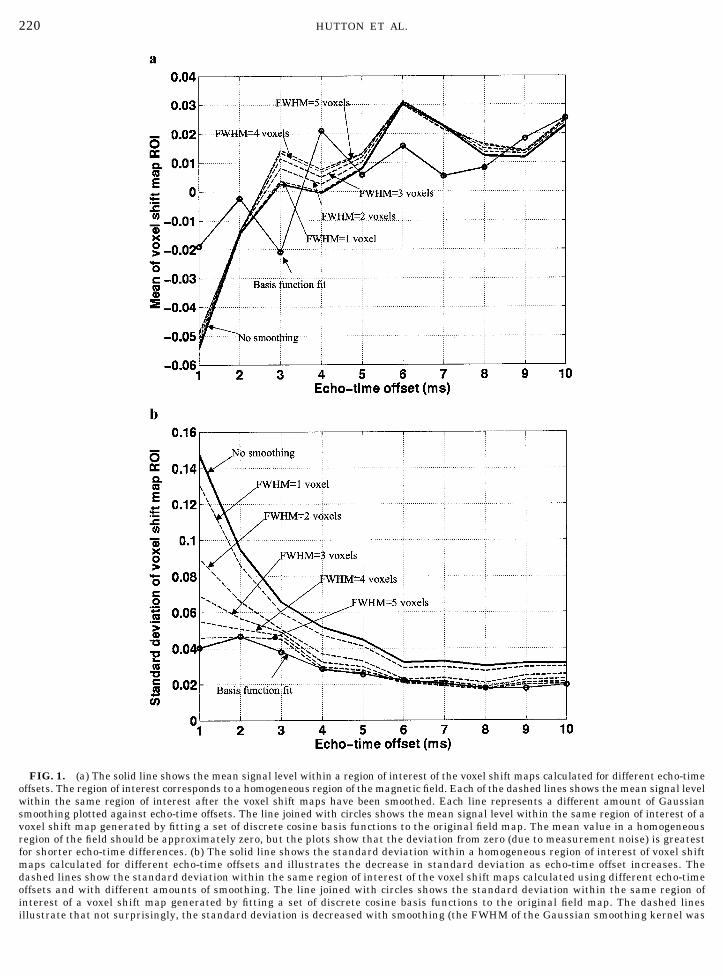
FIG. 1. (a) The solid line shows the mean signal level within a region of interest of the voxel shift maps calculated for different echo-timeoffsets. The region of interest corresponds to a homogeneous region of the magnetic field. Each of the dashed lines shows the mean signal levelwithin the same region of interest after the voxel shift maps have been smoothed. Each line represents a different amount of Gaussiansmoothing plotted against echo-time offsets. The line joined with circles shows the mean signal level within the same region of interest of avoxel shift map generated by fitting a set of discrete cosine basis functions to the original field map. The mean value in a homogeneousregion of the field should be approximately zero, but the plots show that the deviation from zero (due to measurement noise) is greatestfor shorter echo-time differences. (b) The solid line shows the standard deviation within a homogeneous region of interest of voxel shiftmaps calculated for different echo-time offsets and illustrates the decrease in standard deviation as echo-time offset increases. Thedashed lines show the standard deviation within the same region of interest of the voxel shift maps calculated using different echo-timeoffsets and with different amounts of smoothing. The line joined with circles shows the standard deviation within the same region ofinterest of a voxel shift map generated by fitting a set of discrete cosine basis functions to the original field map. The dashed linesillustrate that not surprisingly, the standard deviation is decreased with smoothing (the FWHM of the Gaussian smoothing kernel was
220 HUTTON ET AL.
20 min or more to acquire an fMRI time series ofT2*-weighted images. The time taken to acquire anyadditional scans should therefore be kept to a mini-
mum. A field map based on the acquisition of two EPIvolumes has certain advantages. First, it takes just amatter of seconds to acquire. Second, minimizing the
FIG. 1—Continued
increased from 1 to 5 voxels in unit steps). However, there is a much smaller reduction in standard deviation due to smoothing for field mapsacquired with longer compared with shorter echo-time offsets. (c) Mean image intensity versus echo-time offset within a homogeneous regionof interest after distortion correction with no intensity correction. The plots show the mean of the image intensity after distortion correctionwith the unsmoothed voxel shift map (solid line), with an increasingly smoothed field map (dashed lines), and with the DCT basis functionfit (line joined by circles). The straight line joined by squares represents the mean of the original distorted image. (d) Standard deviation ofimage intensity versus echo-time offset within a homogeneous region of interest after distortion correction with no intensity correction. Theplots show the standard deviation of the image intensity after distortion correction with the unsmoothed voxel shift map (solid line), with anincreasingly smoothed field map (dashed lines), and with the DCT basis function fit (line joined by circles). The straight line joined by squaresrepresents the standard deviation of the original distorted image. (e) Mean image intensity versus echo-time offset within a homogeneousregion of interest after distortion correction with intensity correction. The plots show the mean of the image intensity after distortioncorrection and intensity correction with the unsmoothed voxel shift map (solid line), with an increasingly smoothed field map (dashed lines),and with the DCT basis function fit (line joined by circles). The straight line joined by squares represents the mean of the original distortedimage. (f) Standard deviation of image intensity versus echo-time offset within a homogeneous region of interest after distortion correctionwith intensity correction. The plots show the standard deviation of the image intensity after distortion correction and intensity correctionwith the unsmoothed voxel shift map (solid line), with an increasingly smoothed field map (dashed lines), and with the DCT basis functionfit (line joined by circles). The straight line joined by squares represents the standard deviation of the original distorted image.
221IMAGE DISTORTION CORRECTION IN fMRI
time taken to acquire the two echoes reduces the pos-sibility of artefact due to motion. Finally, the EPI fieldmap will have the same geometric characteristics asthe fMRI data so that unwarping the images involvesminimal processing and linear registration with theEPI data before repositioning voxels along one dimen-sion of the image using linear interpolation.
Decreasing Field Map Noise
As described in Eqs. (1) to (3) above, distortion cor-rection involves scaling the field map, converting it intovoxel shifts that describe the mapping from distortedto undistorted space, then using it to sample the cor-rect points forming the undistorted image. Noise in thecalculated field map will therefore introduce spatialerrors in the undistorted images. In a region of theimage where the magnetic field is uniform, (i.e.,�B0(x, y, z) � 0), there should be no change in positionof the voxels in the corresponding image. However, themeasured field will have measurement noise so thatthe position of a voxel in the corrected image will bedetermined by the field values in the correspondinglocal voxel neighbourhood. Interpolation is required tocalculate the intensity of voxels after adjusting theirposition so that the resulting intensities will also bedependent on field map noise. It is therefore importantto minimize noise in the field map, which can beachieved with the correct choice of acquisition param-eters and with spatial smoothing.
Increasing the echo-time difference of the two im-ages used to calculate the field map increases the sig-nal-to-noise ratio in the acquired phase maps. ForfMRI studies, EPI echo-time is usually selected tomaximise BOLD sensitivity and reduce susceptibility-induced signal loss (Bandettini et al., 1994; Jesmanow-icz et al., 1999). Therefore, if the optimal echo-time isused to acquire the first, longer echo in the field mapacquisition, then the second echo-time should be asshort as possible for two reasons. First, the shorterecho will have less susceptibility-induced signal lossand secondly the echo-time difference will be maxi-mized. This is better than increasing the echo-timedifference by increasing the longer echo-time becausethe increased noise in longer echo-time images woulddominate the noise in the calculated field map.
Different regularisation methods for smoothing fieldmaps have been compared by other authors and theresults suggest that Gaussian smoothing provides thebest regularised field map for distortion correction(Jenkinson, 2001). In this work we wanted to assessthe effect of echo-time difference and spatial smoothingon the signal variance (i.e., noise) in a field map basedon an EPI sequence. We carried out the following ex-periments using a gel phantom. Multislice GE EPIimages were acquired on a Siemens Vision 2T scannerwith matrix size � 64 � 64, FOV � 192 cm, slice
thickness of 1.8 mm with a 1.2-mm gap, TR per slice �76 ms, and 32 slices. A series of EPI images werecollected with echo-times ranging from 40 to 30 ms insteps of 1 ms. A field map was calculated from pairs ofimages for which the longer echo-time was always 40ms and the shorter echo-time was decreased from 39 to30 ms (in 1-ms steps). Field maps were therefore cal-culated with echo-time differences ranging from 1 msto 10 ms (in 1 ms steps). The field maps were scaled asdescribed in Eqs. (1) and (2) and then converted intothe voxel shift maps required for distortion correctionas described in Eq. (3). We use the terms field map andvoxel shift map interchangeably, although in the con-text of distortion correction, it is practical to considerthe field in units of voxel shifts.
We defined a square region of interest (6 � 6 voxelsin one slice) within a homogeneous region of the fieldmap. The mean and standard deviation within theregion of interest were calculated for each of the voxelshift maps (i.e., those calculated with different echo-time offsets) and are illustrated by the solid lines inFigs. 1a and 1b, respectively. The mean value in ahomogeneous region of the field should be approxi-mately zero, but the plots show that the deviation fromzero (due to measurement noise) is greatest for theshorter echo-time difference ( 0.06 voxels). The stan-dard deviation within the region of interest decreasesas the echo-time difference increases ( 0.05 voxels).
Figures 1a and 1b also illustrate the effect of gaus-sian smoothing on noise within a homogeneous regionof the field map. The voxel shift map calculated foreach echo-time difference was smoothed with a three-dimensional Gaussian filter of increasing kernel size.The full width at half-maximum height (FWHM) of thekernel was increased from 1 to 5 voxels in unit steps.The mean and standard deviation of the smoothed fieldwithin the same region of interest as above was mea-sured for the range of smoothing kernels and echo-timeoffsets. The dashed lines in Fig. 1a show that smooth-ing does not have a particularly interesting effect onthe mean value within the homogeneous region of thefield map. Each of the dashed lines in Fig. 1b illus-trates that not surprisingly, the standard deviationdecreases as the smoothing increases. However, thereis a smaller reduction in standard deviation due tosmoothing for field maps acquired with longer com-pared with shorter echo-time offsets. Smoothing istherefore more important for field maps acquired withshorter echo-time offsets.
It is also possible to generate a smoothed version ofthe field map by fitting to it a smoothly varying func-tion. This is particularly advantageous for modellingfield inhomogeneity over the brain because it allowsthe field to be estimated in regions where low signal-to-noise ratio means that the field cannot be accuratelymeasured. The magnetic field varies smoothly overmost regions of the brain but can change more rapidly
222 HUTTON ET AL.
in regions affected by susceptibility artefacts. To modelthese characteristics of the field, Jezzard and Balaban(1995), fit a 2-D polynomial surface to the field map. Inthis work we fit a linear combination of low frequencybasis functions to the field map. We use the eightlowest frequency basis functions (including the con-stant, linear component) of the three-dimensional dis-crete cosine set of transformations (DCT; Jain, 1989) tomodel each spatial dimension. The field is thereforemodelled by a total of 512 (83) basis functions. Thisnumber of basis functions in three dimensions hasbeen chosen empirically for brain images and allowsrapid changes in the magnetic field to be modeled with-out over-fitting to noise or errors in the measuredphase map. Although the DCT basis function model isfitted to the phantom data in this section, the signifi-cance of using this smoothing method for brain imageswill become apparent in the following section.
To observe the smoothing effect of the DCT basis func-tion model versus echo-time difference, the model wasfitted to the phantom field maps calculated above. Themean and standard deviation of the modeled field mapwas calculated within the same region of interest and theresults are illustrated by the lines joined with circles inFigs. 1a and 1b, respectively. The mean of the modeledfield map deviates from zero, although less than the orig-inal and smoothed field maps for shorter echo-time off-sets. At longer echo-time offsets the mean of the modeledfield map varies from the original and smoothed fieldmaps by less than 0.005 voxels. The standard deviation ofthe modeled field map is slightly smaller than that of theoriginal and smoothed field maps.
We used the field maps calculated in the previoussteps to distortion correct the original 40-ms echo-timeimage as described in Eq. (3). Field maps before andafter both gaussian smoothing and DCT basis functionfitting were used for distortion correction to observe
how smoothing the field map influences the correctedimage intensities. Distortion correction was appliedboth with and without the intensity correction de-scribed by Eqs. (4) and (5).
The mean and standard deviation of the distortion-corrected image intensities with and without intensitycorrection were measured within the same region ofinterest as above. Plots of the mean and standarddeviation versus echo-time offset are shown for distor-tion correction without intensity correction in Figs. 1cand 1d, respectively, and with intensity correction inFigs. 1e and 1f, respectively. Each figure shows the meanor standard deviation of the image intensity after distor-tion correction with the unsmoothed voxel shift map (sol-id line), with an increasingly gaussian smoothed fieldmap (dashed lines), and with the DCT basis function fit(line joined by circles). In each figure, the straight linejoined by squares represents the mean or standard devi-ation of the original distorted image.
The results without intensity correction (Figs. 1c and1d) show that both the mean and standard deviation ofthe original image are decreased by all methods ofdistortion correction. For short echo-time offsets thisdecrease is quite abrupt. The mean and standard de-viation are reduced because the distortion correctionitself has a smoothing effect on the image. This iscaused by the interpolation required for the sub-voxelshifts from distorted to undistorted positions [Eq. (3)].The noisier the voxel shift map, the more subvoxelshifting is required for the distortion correction result-ing in a smoother distortion-corrected image. At echotimes longer than 3 ms, there appears to be very littledifference between the results for the different methodsof distortion correction without intensity correction.
The distortion correction results with intensity cor-rection (Figs. 1e and 1f) show that the mean of theoriginal image is increased by all correction methods
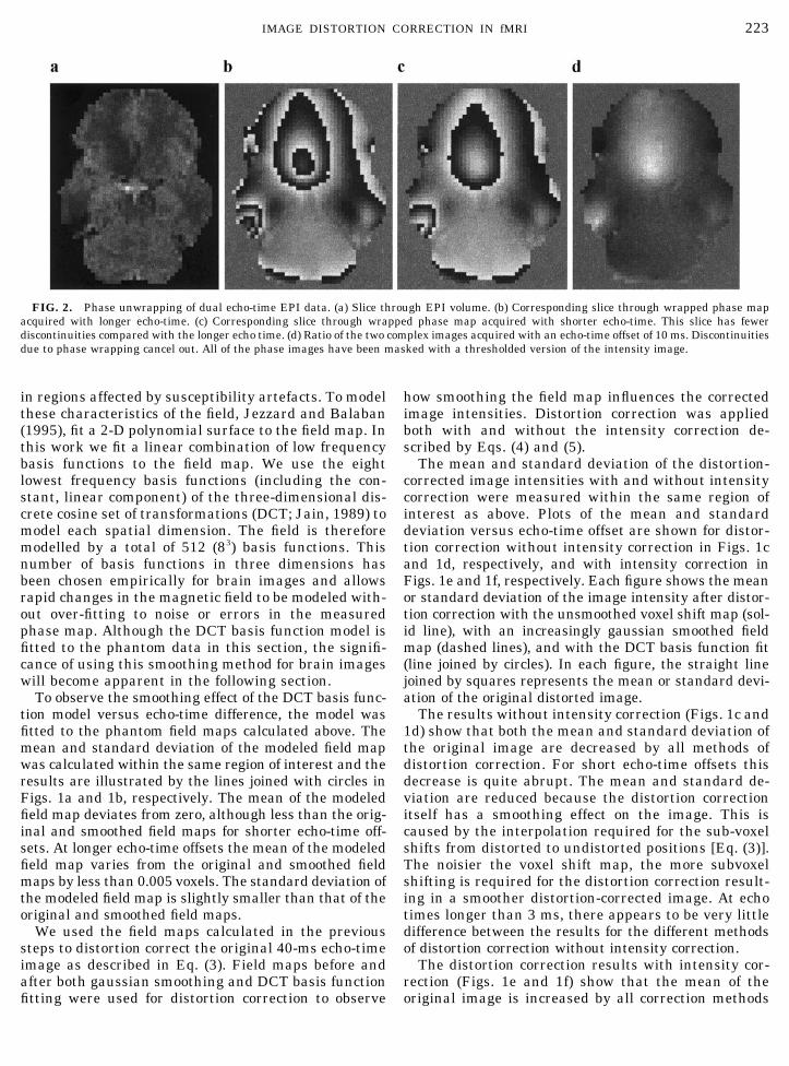
FIG. 2. Phase unwrapping of dual echo-time EPI data. (a) Slice through EPI volume. (b) Corresponding slice through wrapped phase mapacquired with longer echo-time. (c) Corresponding slice through wrapped phase map acquired with shorter echo-time. This slice has fewerdiscontinuities compared with the longer echo time. (d) Ratio of the two complex images acquired with an echo-time offset of 10 ms. Discontinuitiesdue to phase wrapping cancel out. All of the phase images have been masked with a thresholded version of the intensity image.
223IMAGE DISTORTION CORRECTION IN fMRI
for echo-time offsets greater than 2 ms. The standarddeviation of the original image is increased by all meth-ods of distortion correction except for the DCT basisfunction fit. These results suggest that including anintensity correction may increase the noise in the cor-rected image. As described in Eqs. (4) and (5), theintensity correction is based on a function of the one-dimensional derivative of the voxel shift map, which ismultiplied by the image intensity. Therefore, if thevoxel shift map is noisy it is clear that this will resultin an increase in image noise. The DCT basis functionfit is very smooth and therefore an intensity correctionbased on its derivative introduces less image noise.
Phase Unwrapping
The robustness of the calculated field map is depen-dent not only on the noise characteristics of the ac-
quired phase maps but also on the ability to extractreliable phase information from the measured complexdata. The problem is that phase is uniquely definedonly in the principal value range of [�, ]. Any valueoutside this range will be wrapped around so that itsso-called “wrapped phase” is offset from its actualphase by an integer multiple of 2. Phase wrappingcan be detected as spatial discontinuities in the phasemap and can be “unwrapped” by adding or subtractingmultiples of 2 to the voxels where these discontinui-ties occur. The addition and subtraction of multiples of2 can be arbitrary over the image. It is thereforeimportant to correctly define where in the image the“wrapped phase” offset is zero. This can be achieved bydefining a starting point for the phase unwrapping thatcorresponds to the most uniform region of the magneticfield, i.e., where the field should be approximately zero.
FIG. 3. (a–c) Each row contains a slice from the intensity image (left) corresponding to a low-noise mean field map (second column), the basisfunction fit to the mean field map (third column), and the gaussian smoothed (FWHM � 1 voxel) mean field map (right) for (a) an upper slice, (b)a middle slice, and (c) a lower slice in the brain. The dashed lines through the intensity image slices represent the position of the profiles throughthe corresponding field maps, which are plotted in d–f. (d–f) Profiles through the field maps shown in a–c, respectively. The solid line is a plot ofthe profile through the mean field map. The dashed lines are plots through the mean field map after increased levels of gaussian smoothing(FWHM � 1 to 5 voxels). The line joined with circles is a plot through the basis function fit to the mean field map.
224 HUTTON ET AL.
Discontinuities due to phase wrapping can be mini-mised by computing the phase map from the ratio oftwo complex images acquired with different echo-
times. This is equivalent to finding the difference be-tween the two phase components of the complex im-ages (i.e., the phase evolution between the two echo-times). If the time between the two echoes is not toolong, the phase offset of many of the “phase wrapped”voxels will be the same in the two echoes and willcancel out in the ratio of the two complex images. Thiswill reduce the number of voxels that require phaseunwrapping or eliminate them altogether. However, asshown in the previous section, a longer echo-time offsetyields improved signal-to-noise in the measured fieldmap. Therefore a trade-off must be found betweenthese two factors. Figure 2 illustrates the calculation ofa phase map using a dual echo-time EPI acquired witha 10-ms offset. The figure shows that no phase unwrap-ping is necessary once the ratio of the two compleximages has been computed.
Even with minimal phase discontinuities, phase un-wrapping algorithms may not be completely robustwhen applied to noisy three-dimensional EPI data. EPIimages of the brain present specific difficulties becauseof the brain anatomy and susceptibility artefacts. Ingeneral, phase unwrapping algorithms use the condi-tion that the phase difference between adjacent voxelsshould be less than radians (Axel and Morton, 1989;Hedly and Rosenfeld, 1992). This condition is sensitiveto noise and is particularly a problem in regions of lowsignal intensity. It is also dependent on spatial conti-nuity across the object within the image. Phase un-wrapping is usually reliable in the upper slices of thebrain, where there are spatially continuous regionswithin each slice. In the lower slices of the brain whereregions appear to be spatially disconnected, either be-cause of the anatomy of that region or susceptibilityinduced signal loss, phase unwrapping is less reliable.More sophisticated approaches to phase-unwrappinghave been proposed (Cusack et al., 1995, 2001), whichmay provide improved results in the presence of dis-continuities caused by noise. In general many unwrap-ping algorithms are not completely fail-safe and re-quire some heuristic measures to ensure that the finalfield map does not contain any errors.
Creating a Field Map of the Brain
We describe a method for generating field maps ofthe brain that has been applied successfully in thiswork. Voxels must be spatially connected for successfulphase unwrapping. Therefore we create an intensitymask based on the spatial connectivity of voxels as wellas grey level intensity by labelling all voxels above aspecified threshold (based on the mean intensity of theimage) that are connected with all other voxels in theobject. The spatial connectivity mask will contain mostof the brain but will exclude regions that appear to bedisconnected in the image such as eyeballs and inferiorfrontal regions. This mask is generated using the
FIG. 3—Continued
225IMAGE DISTORTION CORRECTION IN fMRI
longer echo-time image, which will have the most sus-ceptibility-induced signal loss. Multiplying the phasemap by this mask will therefore ensure robust phaseunwrapping within spatially connected regions of thebrain resulting in an unwrapped phase map that canbe scaled and converted to a voxel shift map using Eqs.(1) and (2). The resulting masked field map can be usedfor distortion correction as described in Eq. (3), butbecause of anatomy or signal loss some disconnectedbrain regions or regions with low signal intensity willbe excluded from the resulting unwrapped phase map.We therefore fit the DCT basis function model de-scribed under “Decreasing field map noise” to thismasked field map. Outside of the masked regions thefunction will vary smoothly and slowly providing anestimation of the phase. We then create a second in-tensity mask based on a thresholded version of theimage acquired at the shorter echo-time which has lesssusceptibility-induced signal loss (again with thethreshold based on the mean image intensity). Thesecond mask is not dependent on spatial connectivityin the brain and is used to identify brain regions thatwere excluded by the first mask.
By masking the basis function model fit with thesecond mask we can estimate the phase in regions ofthe brain excluded by the first mask. There still will beregions of the brain where phase information is miss-ing due to susceptibility induced signal loss. However,as there is no EPI signal in these regions it is onlynecessary to constrain the modelled phase map to fallsmoothly to a value of zero. This is assuming that thephase unwrapping correctly defined the zero offset tocorrespond to a region where the field inhomogeneity isapproximately zero as described under “Phase unwrap-ping.” This is achieved by dilating and smoothing thesecond mask as described in Jezzard and Balaban(1995). The result provides a model of the field inho-mogeneity over the whole brain with minimal noiseand errors, which can be converted into a map of voxelshifts and used to unwarp the distorted images.
Decreasing Noise in Field Maps of the Brain
The previous results demonstrate the effect of spa-tial smoothing within a homogeneous region of a phan-tom field map. However, the magnetic field within ahuman brain has more inhomogeneities so that spatialsmoothing of the field map may cause artifactual blur-ring in regions where the field changes rapidly. Toinvestigate this effect, we constructed a low-noise ref-erence field map by acquiring a series of 50 dual echo-time EPI images. Each pair of images had echo-timesequal to 40 and 30 ms. All other acquisition parameterswere the same as described in the previous section.During the scanning session, the subject remained asstill as possible.
An unwrapped phase map was calculated from eachpair of EPI images by creating a spatial connectivitymask from a 40 ms echo-time image, masking thenunwrapping the phase maps as described under “Cre-ating a field map of the brain.” The 40 ms echo-timeintensity images were registered using SPM’99 (http://www.fil.ion.ucl.ac.uk). The resulting motion parame-ters were used to coregister the unwrapped phasemaps and create a mean phase map. After scalingusing Eqs. (1) and (2), a low-noise mean field (voxelshift) map was generated in which spatial variationswere mostly due to real variations in the magnetic fieldrather than measurement noise. This made it possibleto assess any artifactual effects of smoothing, espe-cially in regions of the brain where there are rapidchanges in the magnetic field.
The mean field map was smoothed with a three-dimensional Gaussian filter of increasing kernel size(FWHM from 1 to 5 voxels). The DCT basis functionmodel was fitted to the mean field map and an in-tensity mask based on a 30-ms echo-time image wasused to mask the model fit as described under “Cre-ating a field map of the brain.” The resulting mod-eled field map gave an estimation of the field inregions excluded by the original unwrapped phasemaps.
Figure 3 shows an upper (a), middle (b), and lower (c)slice from the mean field map (second column), thebasis function fit (third column), and the field mapafter gaussian smoothing with a kernel FWHM � 1voxel (fourth column). The corresponding intensity im-age slices are also shown in the first column. Repre-sentative profiles in the phase encoding directionthrough the field maps for the upper, middle, and lowerslices are shown in Figs. 3d, 3e, and 3f, respectively.The dashed line on each intensity image in Figs. 1a–1cindicates the position of the corresponding profile foreach slice.
The profiles demonstrate that in regions where thefield varies slowly, the smoothed and modeled fieldmaps do not deviate from the mean field map. In re-gions where the field changes rapidly, the fieldsmoothed with a gaussian kernel, FWHM � 1 voxeldeviates from the mean field by 0.1 voxels (e.g., at thepeak values in Figs. 3d–3f). However, more gaussiansmoothing and modelling cause artifactual blurring inregions where the field changes rapidly. The field mapsmoothed with gaussian FWHM � 5 voxels and themodelled field map can deviate by up to 1 voxel fromthe mean field map (as shown by the peak in Fig. 3e).It should be noted that regions where the field changesrapidly often correspond to low signal to noise ratio inthe image where inaccuracies in the distortion correc-tion are least noticeable.
The advantage of the basis function model is that itcan provide an estimation of the field in regions where
226 HUTTON ET AL.
it can not be measured. This is demonstrated in theregion of the sinus in Fig. 3b and the eyeballs in Fig. 3c.
DISTORTION CORRECTION AND ANATOMICALCOREGISTRATION
Other authors have demonstrated that a significantamount of geometrical distortion due to susceptibilityartefacts can be corrected using a field map. In thissection we show how even small geometric distortions,on the order of 1 or 2 voxels, can cause a noticeablemismatch between functional and anatomical images.To demonstrate the effect of distortion correction onanatomical coregistration it is necessary to considerthe relationship between the EPI image and the ana-tomical image. If an EPI and an anatomical image fromthe same subject are free of geometric distortions thenit can be assumed that the transformation required tocoregister these images will be linear, containing onlytranslations, rotations, and scaling to compensate fordifferences in voxel size. Therefore the transformationrequired to match a correctly unwarped EPI image tothe corresponding anatomical image should also be alinear transformation. In contrast, the transformationrequired to match a distorted EPI image with the an-atomical image will contain nonlinear terms in thedirection of the distortion. A linear registration be-tween an undistorted image and the correspondinganatomical image should therefore result in a bettermatch compared to a linear registration between thedistorted image and the anatomical image.
In this work, we used a multimodality coregistrationmethod based on information theory to linearly coreg-ister the distorted and undistorted images to the ana-tomical image. This coregistration method uses the“mutual information” of the two images as a matchingcriterion. It is based on the work by Collignon et al.(1995) and is implemented in SPM’99 (http://www.fil.ion.ucl.ac.uk). This method maximizes the relativeentropy of the joint intensity distribution of two imagesand provides a quantitative measure (the “entropy cor-relation coefficient”), representing the degree of inter-dependence of the two images. This measure can beused to compare the maximized mutual informationbetween the EPI and the anatomical image before andafter distortion correction. It therefore provides a mea-sure to determine whether the distorted or the undis-torted image better matches the anatomical image.
Methods
The effect of distortion correction on anatomicalcoregistration is demonstrated for three subjects. An-atomical images with isotropic 1 mm voxel resolutionwere acquired using a centric-ordered phase-encodeMP-RAGE sequence optimised for grey and white mat-ter contrast (Deichmann et al., 2000). Dual echo-timeEPI images were acquired using multislice GE EPIwith matrix size � 64 � 64, FOV � 192 cm, slicethickness � 1.8 mm with a 1.2-mm gap, TR per slice �76 ms and 48 slices. Two images were acquired withdifferent echo-times of TE � 40 ms and TE � 27 ms.Fat suppression was used to reduce the presence ofsignal from fat in the images. Images were acquired ona Siemens Vision 2T scanner. The EPI images werereconstructed using a novel trajectory-based methodthat substantially decreases Nyquist ghost artefacts(Josephs et al., 2000).
Unwrapped phase maps were created as describedunder “Creating a field map of the brain.” Fieldmaps were then generated using two processingmethods (F1) gaussian smoothing, FWHM � 1 voxeland (F2) fitting with DCT basis functions as de-scribed under “Creating a field map of the brain.”The smoothed field map (F1) and the modeled fieldmap (F2) were converted into maps of voxel shifts inundistorted image space then used to correct thedistorted EPI images acquired with TE � 40 msusing Eq. (3). Both distortion corrections were ap-plied with and without intensity correction (IC) asdescribed by Eqs. (4) and (5), resulting in four cor-rected EPI images for each subject (corrected usingF1, F1 � IC, F2, F2 � IC).
The distorted and each of the corrected EPI imageswere independently coregistered to the correspond-ing subject’s anatomical image using the ‘mutualinformation’ coregistration method implemented inSPM’99 (http://www.fil.ion.ucl.ac.uk). The “entropycorrelation coefficient,” a measure of the interdepen-dence of the two images was computed for each set ofcoregistered images. The coregistration was per-formed for EPI images after distortion correctionusing F1, F1 � IC, F2, and F2 � IC. Each of thedistortion-corrected images was subtracted from thedistorted images after coregistration to highlight dif-ferences due to the correction.
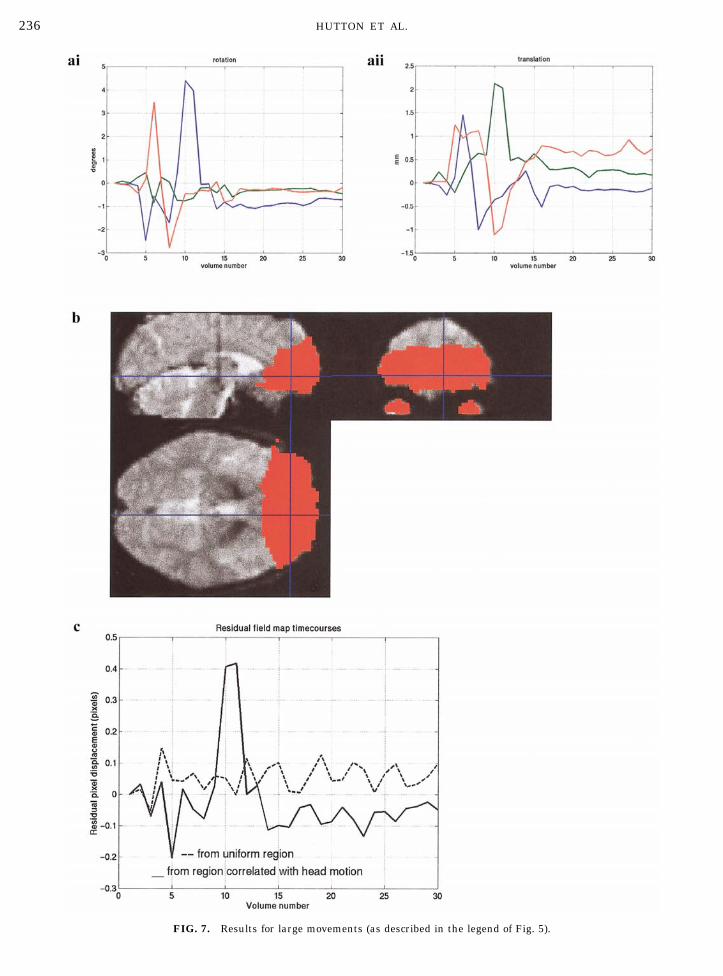
FIG. 4. Results of anatomical coregistration. Two slices from the brain are shown for each of the three subjects (subject 1, a and b; subject2, c and d; subject 3, e and f). (Column I) Subtraction of the corrected EPI image using F1 � IC from the original distorted EPI image. Thebright regions indicate where signal in the distorted image is greater than the corrected image and dark regions the opposite. (Column II)Contours of the coregistered distorted (red) and corrected images (F1, pale blue; F1 � IC, dark blue) overlaid on the anatomical image. (ColumnIII) Contours of the coregistered distorted (red) and corrected images (F2, yellow; F2 � IC, dark blue) overlaid on the anatomical image. (ColumnIV) Smoothed field map. (Column V) Fitted field map. The grey scale bar indicates the size of the measured distortion in voxels with bright values,indicating distortion toward the top of the page and dark values, indicating distortion toward the bottom of the page.
227IMAGE DISTORTION CORRECTION IN fMRI
FIGURE 4
228 HUTTON ET AL.
Results
The results from the anatomical coregistration areshown in Fig. 4. Two slices from the brain are shownfor each of the three subjects (subject 1, a and b; subject2, c and d; subject 3, e and f). Shown for each subject isa more superior slice in the brain where there aresmaller and more typical distortions (a, c, and e) andan inferior slice where the distortion is greatest (b, d,and f). Column I shows the subtraction of the correctedEPI image using F1 � IC from the original distortedEPI image. Bright regions indicate where signal in thedistorted image is greater than the corrected imageand dark regions the opposite. All the subtraction im-ages for the different correction methods showed asimilar pattern of differences. For compactness, onlythe subtraction results for the F1 � IC correction areshown. These subtraction images indicate where thereare differences resulting from the intensity correctionas well as the distortion correction. Columns II and IIIshow contours of the distorted and corrected imagesoverlaid on the coregistered anatomical image. Theanatomical image has been sampled at the resolutionof the EPI images. The contours were calculated usingthe contour function in Matlab (Matlab 5.3.1, 1999),which draws curves joining together points in the im-age with the same value. In column II, the red contourcorresponds to the distorted EPI image, the pale bluecontour corresponds to the corrected image using F1and the dark blue contour corresponds to the correctedimage using F1 � IC. In column III, the red contouragain corresponds to the distorted EPI image, the yel-low contour corresponds to the corrected image usingF2 and the dark blue contour corresponds to the cor-rected image using F2 � IC. Columns IV and V showthe smoothed field map and the fitted field map respec-tively. The grey scale bar indicates the size of themeasured distortion in voxels with bright values indi-cating distortion towards the top of the page and darkvalues indicating distortion towards the bottom of thepage.
The mismatch between the contours in columns IIand III illustrates the mismatch between the distortedand corrected images. In many regions the scale of themismatch corresponds to the scale of the distortionshown in columns IV and V. In the more superior slicesof the brain (a, c, and e), the distortion is of the order of1 to 1.5 voxels (3–4.5 mm) and causes an apparentstretching of the image slice. The distortion correctionappears to work well in such regions. In the moreinferior slices where there are more severe susceptibil-ity artefacts (b, d, and e), the scale of the distortionapproaches 2–3 voxels (6–9 mm). The maximum dis-tortion occurs in regions where there is almost totalsignal loss as demonstrated by the contours around theinferior frontal regions in slices b and d. It is therefore
difficult to assess the effect of the distortion correctionin these regions.
There are no obvious visible differences in coregis-tration for the different distortion correction methods(F1 and F2, pale blue and yellow contours in columns IIand III, respectively). The difference between distor-tion correction with and without intensity correction ismost apparent in slice b, around the inferior temporalregions.
Coregistration using “mutual information” providesa visibly good match between the anatomical and EPIimages (both before and after distortion correction).The Entropy Correlation Coefficients given in Table 1allow the coregistration of anatomical images to dis-torted and corrected images to be compared. For allsubjects, distortion correction without intensity correc-tion (F1 and F2) improved the coregistration results. Insubjects 1 and 2, distortion correction with intensitycorrection (F1 � IC and F2 � IC) also improved thecoregistration results. These results suggest that over-all there is a greater level of interdependence andtherefore a better match between the functional andanatomical images after distortion correction. Al-though there was not one method that was consistentlybetter in all data sets, only in subject 1 did the correc-tion method F2 give a better fit than F1 and only insubject 2 was the coregistration improved by intensitycorrection for both distortion correction methods.
DISTORTION CORRECTION AND HEAD MOTION
Previous work has demonstrated that geometric dis-tortions are modulated by head motion (Jezzard andClare, 1999). The field inhomogeneity should thereforebe considered as having a constant component and atime-varying component due to head motion. The re-sulting time-varying distortions can be characterizedby generating a field map at each time point. We useda dual echo-time EPI sequence that provided two im-ages at each time point. It was therefore possible tocalculate a unique field map corresponding to the headposition at each time point. This time series allowed usto characterise and evaluate the interaction of distor-tion with head motion and to test whether the varianceintroduced by the interaction between distortion andhead motion could be removed by distortion correctionwith a time-varying field map.
TABLE 1
Original F1 F1 � IC F2 F2 � IC
Subject 1Figs. 4a and 4b 0.1925 0.1954 0.1952 0.1964 0.1942
Subject 2Figs. 4c and 4d 0.1927 0.1977 0.1999 0.1968 0.1982
Subject 3Figs. 4e and 4f 0.2324 0.2359 0.2312 0.2356 0.2310
229IMAGE DISTORTION CORRECTION IN fMRI
FIGURE 5
230 HUTTON ET AL.
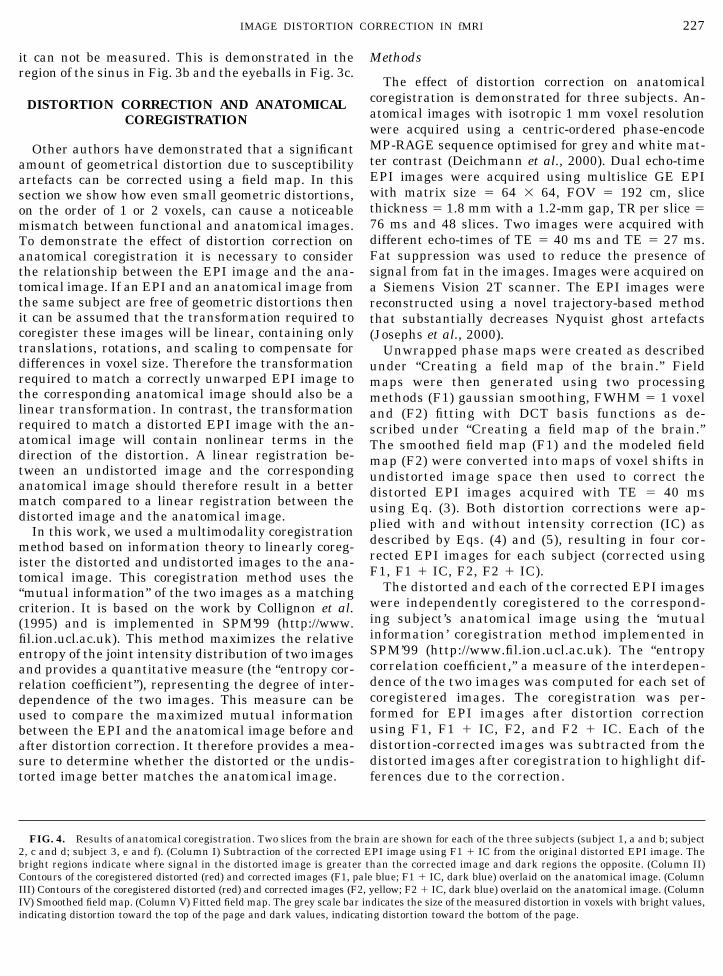
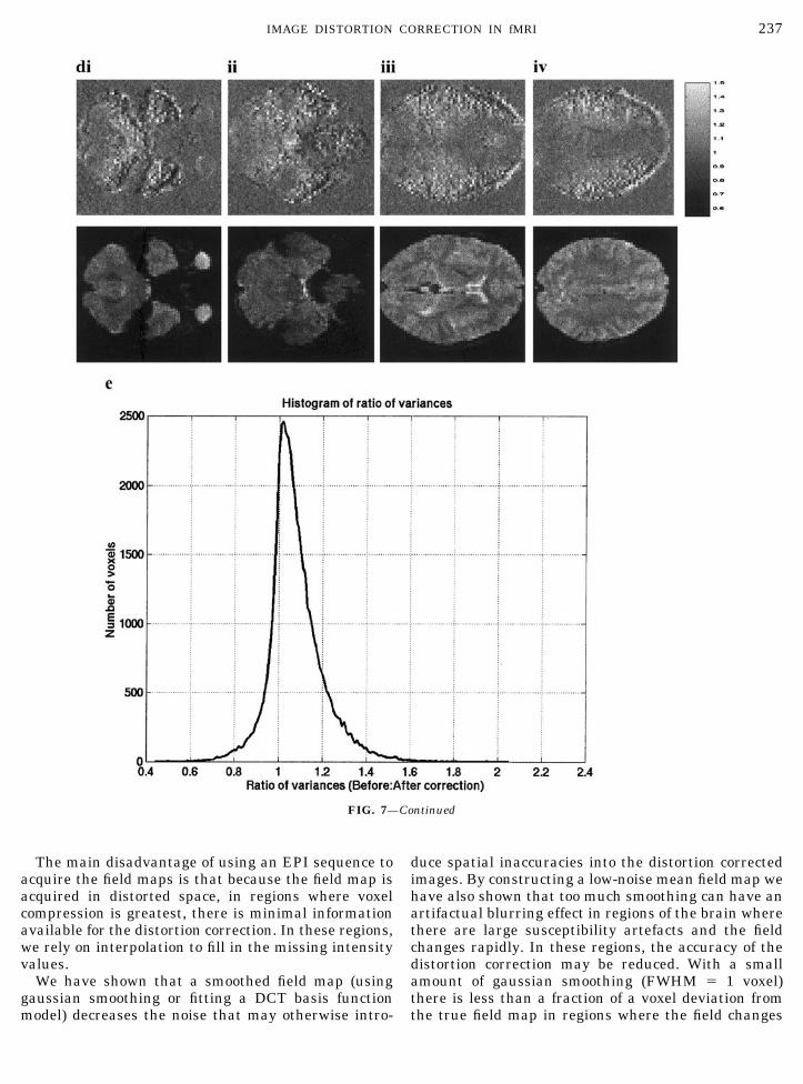
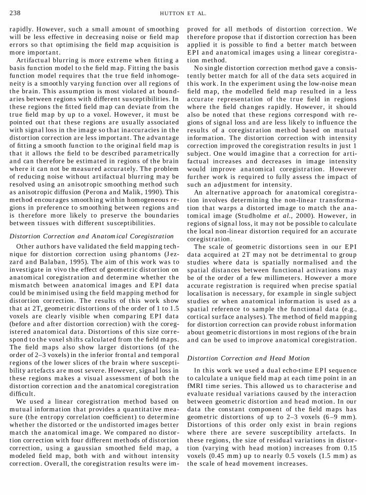
FIG. 5. Results for small movements. (a) Motion parameters for (i) rotation (about x-axis, blue; y-axis, green; z-axis, red) and (ii)translation (in x, blue; y, green; z, red). (b) Regions of the brain where distortion is significantly correlated with head motion. The overlaidstatistics are thresholded at P 0.001 (uncorrected for multiple comparisons). (c) Voxel timecourses through realigned residual field maps(scaled to represent voxel shifts). The dashed line shows a timecourse from a region where the magnetic field is nearly uniform and there isno correlation with head motion. The solid line shows a timecourse from a region where there is a significant correlation with head motion.(d) Slices from the quotient of the variance maps before and after distortion correction with the corresponding image slices in the bottom row.The grey-scale bar corresponds to the quotient values and the background of the image has been set to 1. Values �1 (brighter than thebackground) correspond to a decrease in variance due to distortion correction, values 1 (darker than the background) correspond to anincrease in variance due to distortion correction and values � 1 correspond to no change in variance. (e) Histogram of quotient of variances.
231IMAGE DISTORTION CORRECTION IN fMRI
FIG. 6. Results for medium movements (as described in the legend of Fig. 5).
232 HUTTON ET AL.
MethodsDual echo-time EPI images were acquired with the
same parameters as described in the previous section.The images were acquired during short scanning ses-sions (about 3 min) for two different subjects. Duringeach session the subject was first asked to keep as stillas possible, then to move his head slightly and finallyto move his head more. A field map was calculated from
each pair of images in the time series and modeled byfitting DCT basis functions as described under “Creat-ing a field map of the brain.” A visual check was madeto ensure that all field maps in the time series had beensensibly unwrapped and modelled. Each modeled fieldmap was then used to correct for distortions in thecorresponding image (the images with the longer echo-time (TE � 40 ms) were corrected). Intensity correction
FIG. 6—Continued
233IMAGE DISTORTION CORRECTION IN fMRI
was also applied to the distortion-corrected images asdescribed by Eqs. (4) and (5).
Using SPM’99 the original image volumes were re-aligned to the first in the time series. The estimatedmotion parameters (three translations and three rota-tions) were then used to realign the field maps. Asimple regression analysis was performed between therealigned field maps and the motion parameters todetect voxels for which the time courses in the re-aligned field maps were correlated with head move-ment. Movement correlated changes in the realignedfield maps will correspond to time-varying changes inthe distorted time-series. This analysis therefore iden-tified regions in the brain where there was a significantinteraction between head motion and geometric distor-tion. SPM’99 was used to create maps of F statistics toshow the voxel-wise correlation between the field mapsand the motion parameters. Voxels that survived a Pvalue threshold of P 0.001 (uncorrected for multiplecomparisons) were considered to be significantly corre-lated with head motion. Our hypothesis was that brainregions affected by the interaction between distortionand head motion would be in areas where the constantcomponent of the field inhomogeneity deviated mostfrom zero (i.e., in areas most severely affected by sus-ceptibility artefacts). These regions are near tissueboundaries where the field is most likely to vary as thehead changes position.
The first field map in the time series was subtractedfrom the rest of the realigned field maps to generate atime series of residual field maps. Residual timecourses were extracted from regions of the field mapwhere (a) the magnetic field was nearly uniform and (b)there was a significant correlation with head motion.These time courses (in voxel displacements) were usedto indicate the amplitude of the time-varying compo-nent of the field maps (i.e., the change in distortion dueto motion).
Finally the images after distortion correction wererealigned. The variance of each realigned image timeseries before and after distortion correction was calcu-lated. A quotient of variance image was calculated foreach pair of variance images, dividing the variancebefore by the variance after distortion correction.Where the quotient is greater than 1, the variance hasbeen decreased by distortion correction and where thequotient is less than 1, the variance has been increasedby distortion correction. Quotient values of 1 indicateno difference in the variance before and after distortioncorrection. A histogram of the quotient values was alsoconstructed.
The data from the two subjects gave a range of dif-ferent scales of head movements, which were then clas-sified according to the scale of head motion. The clas-sifications were small ( �0.2° and �0.2 mm),medium ( �1° and �1 mm) and large movements
( �5° and �2.5 mm). One set of results is shown foreach range of movements.
Results
Results are shown from the first subject for smallmovements (Fig. 5) and for the second subject for me-dium and large movements (Figs. 6 and 7). These re-sults do not represent all of the acquired data but aretypical of the data classified with corresponding scalesof movement.
For each of the quotient of variance maps (Figs. 5e,6e, and 7e) there is a corresponding grey-scale bar. Thebackground of each of the quotient of variance imageshas been set to 1. Therefore values �1 (brighter thanthe background) correspond to a decrease in variancedue to distortion correction, values 1 (darker than thebackground) correspond to an increase in variance dueto distortion correction and values � 1 correspond to nochange in variance.
Small movements (� �0.2° and �0.2 mm—Fig.5a). Less than 3% of voxels in the brain show a sig-nificant correlation with head motion (Fig. 5b). Thesevoxels occur in the vicinity of the air-filled sinus in theinferior frontal region. They are mainly correlated withrotation about the x-axis and translation in the y- andz-axis.
The time course from a uniform region of the fieldmap (Fig. 5c, dashed line) shows that residual voxeldisplacements vary by up to 0.12 voxels (0.36 mm).Similarly, the time course from the inferior frontalregion (which is correlated with head motion, Fig. 5c,solid line) shows that residual voxel displacementsvary by up to 0.15 voxels (0.45 mm).
Slices from the quotient of variance maps before andafter distortion correction are shown in Figs. 5d (i–iv)together with the corresponding image slices. Theseillustrate that most voxels in the displayed slices havea value greater than 1 representing a global decreasein variance due to distortion correction. This is alsoevident in the histogram (Fig. 5e), which has a peakvalue at around 1.1. There are also regions where thedistortion correction has increased the variance. Thisis evident in the region of the sinus (Figs. 5di and 5dii)and is probably due to the severe signal dropout andinaccuracies in the field map in this region. In Figs.5diii and 5div there are contour shaped areas wherethe quotient of variance value is approximately equalto 1 (no change in variance). These regions correspondto zero crossings in the field maps where the field isrelatively uniform and therefore distortion correctionhas not changed the images.
Medium movements ( �1° and �0.6 mm—Fig.6a). Less than 4% of voxels in the brain show a sig-nificant correlation with head motion (Fig. 6b). Thesevoxels occur in the frontal lobes and eyeballs. Thetimecourse from a uniform region of the field map (Fig.
234 HUTTON ET AL.
6c, dashed line) shows that residual voxel displace-ments vary by nearly 0.2 voxels (0.6 mm). The timecourse from the frontal region (Fig. 6c, solid line) showsthat residual voxel displacements vary by up to 0.3voxels (0.9 mm). The realignment parameters illus-trate that this time course is clearly correlated withtranslation in the z-axis (Figs. 6aii, red line).
Slices from the quotient of variance maps before andafter distortion correction are shown in Figs. 6d (i–iv),together with the corresponding image slices. Theseillustrate that in all slices there are some regions ofdecreased variance (brighter voxels) away from thecentral regions of the brain. In particular the decreasein variance is illustrated by the bright region at thefront edge of the brain corresponding to areas that areparticularly vulnerable to distortion by movement ef-fects. There are also some regions of increased variancedue to distortion correction in regions affected by sig-nal loss (i.e., dark voxels around the temporal lobesand sinuses in Figs. 6di and dii). The histogram ofquotient values (Fig. 6e) has a peak at a value fraction-ally greater than 1, indicating that slightly more voxelsshow a decrease in variance due to distortion correc-tion.
Large movements ( �5° and �2.5 mm—Fig. 7a).Around 10% of voxels in the brain show significantcorrelation with head motion (Fig. 7b). These voxelsoccur in a large portion of the frontal lobes and in theeyeballs. The timecourse from a uniform region of thefield map (Fig. 7c, dashed line) shows that residualvoxel displacements vary by up to 0.2 voxels (0.6 mm).The time course from the frontal region (Fig. 7c, solidline) shows that residual voxel displacements vary byup to 0.6 voxels (1.8 mm). The realignment parametersillustrate that this time course is clearly correlatedwith rotation about the x-axis (Fig. 7ai, blue line) andtranslation in the y- and z-axis (Fig. 7aii, green and redlines).
Slices from the quotient of the variance maps beforeand after distortion correction are shown in Fig. 7d(i–iv), together with the corresponding image slices.The pattern of decreases and increases in variance aresimilar to those in Fig. 6d. The edges of the brain (inparticular at the front) show the greatest decrease invariance due to distortion correction. Around the mid-dle of the brain there are regions where the quotient ofthe variance before and after distortion correction isapproximately 1. This corresponds to uniform regionsof the magnetic field where there is minimal distortion.Figures 7di and 7dii show regions of increased variancedue to distortion correction, which as before correspondto regions affected by signal loss. Again, the histogramof quotient values (Fig. 7e) has a peak at a valuefractionally greater than 1, indicating that slightlymore voxels show a decrease in variance due to distor-tion correction.
In all of the results, the decrease in variance may bedue to the smoothing effect of voxel resampling in theunwarping process in addition to the realignment andreslicing of the distortion corrected images. The resultsshowed that even in uniform regions, the residualchanges in the field maps were as large as 0.2 voxels(0.6 mm). These residual changes may be due to mea-surement noise or differences in the modeled fieldmaps and may explain some of the increases in vari-ance. Both increases and decreases in variance mayalso be caused by the intensity correction applied tocorrect for changes in voxel brightness. The aim of theintensity correction is to adjust intensity values thathave been increased or decreased by distortion. How-ever, the small local increases or decreases in intensitywill correspond to small increases or decreases in vari-ance with respect to the original images. A more thor-ough assessment of the positive and negative effects ofintensity correction would be an interesting avenue forfurther work. In a comparison of different unwarpingmethods using regularised B0 maps (Jenkinson, 2001),intensity correction was not shown to improve the dis-tortion correction.
DISCUSSION
In this paper we have assessed the effect of imagedistortion correction for fMRI at 2T. This field mappingmethod of distortion correction is well understood, andrelatively quick and simple to implement. We haveexplored how this method can be optimized to acquirerobust field maps, investigated field map smoothingand have quantified the effect of distortion correctionon anatomical coregistration. We have also investi-gated whether the field mapping technique can be usedto correct for the interaction between geometric distor-tion and head motion in fMRI time series.
Field Map Acquisition and Calculation
We have shown that a dual echo-time EPI sequencecan be used to acquire and calculate robust field maps.Using this fMRI sequence to acquire the field map datameans that the field map and the fMRI data will sharethe same geometric properties. The field map willtherefore provide an accurate representation of thevoxel shifts that can be applied with minimal process-ing to fMRI data. The longer echo-time of the dualecho-time sequence should be equal to that used forfMRI scanning. This echo-time is usually chosen tooptimise the sensitivity of detection of BOLD signal,i.e., the echo-time is approximately equal to the T2* ofgrey matter at a particular field strength (Bandettini etal., 1994). The shorter echo time should be chosen sothat the echo-time difference is long to minimise fieldmap noise but short enough to allow robust phaseunwrapping. We have found an echo time offset ofaround 10 to 15 ms to be appropriate in this work.
235IMAGE DISTORTION CORRECTION IN fMRI
FIG. 7. Results for large movements (as described in the legend of Fig. 5).
236 HUTTON ET AL.
The main disadvantage of using an EPI sequence toacquire the field maps is that because the field map isacquired in distorted space, in regions where voxelcompression is greatest, there is minimal informationavailable for the distortion correction. In these regions,we rely on interpolation to fill in the missing intensityvalues.
We have shown that a smoothed field map (usinggaussian smoothing or fitting a DCT basis functionmodel) decreases the noise that may otherwise intro-
duce spatial inaccuracies into the distortion correctedimages. By constructing a low-noise mean field map wehave also shown that too much smoothing can have anartifactual blurring effect in regions of the brain wherethere are large susceptibility artefacts and the fieldchanges rapidly. In these regions, the accuracy of thedistortion correction may be reduced. With a smallamount of gaussian smoothing (FWHM � 1 voxel)there is less than a fraction of a voxel deviation fromthe true field map in regions where the field changes
FIG. 7—Continued
237IMAGE DISTORTION CORRECTION IN fMRI
rapidly. However, such a small amount of smoothingwill be less effective in decreasing noise or field maperrors so that optimising the field map acquisition ismore important.
Artifactual blurring is more extreme when fitting abasis function model to the field map. Fitting the basisfunction model requires that the true field inhomoge-neity is a smoothly varying function over all regions ofthe brain. This assumption is most violated at bound-aries between regions with different susceptibilities. Inthese regions the fitted field map can deviate from thetrue field map by up to a voxel. However, it must bepointed out that these regions are usually associatedwith signal loss in the image so that inaccuracies in thedistortion correction are less important. The advantageof fitting a smooth function to the original field map isthat it allows the field to be described parametricallyand can therefore be estimated in regions of the brainwhere it can not be measured accurately. The problemof reducing noise without artifactual blurring may beresolved using an anisotropic smoothing method suchas anisotropic diffusion (Perona and Malik, 1990). Thismethod encourages smoothing within homogeneous re-gions in preference to smoothing between regions andis therefore more likely to preserve the boundariesbetween tissues with different susceptibilities.
Distortion Correction and Anatomical CoregistrationOther authors have validated the field mapping tech-
nique for distortion correction using phantoms (Jez-zard and Balaban, 1995). The aim of this work was toinvestigate in vivo the effect of geometric distortion onanatomical coregistration and determine whether themismatch between anatomical images and EPI datacould be minimised using the field mapping method fordistortion correction. The results of this work showthat at 2T, geometric distortions of the order of 1 to 1.5voxels are clearly visible when comparing EPI data(before and after distortion correction) with the coreg-istered anatomical data. Distortions of this size corre-spond to the voxel shifts calculated from the field maps.The field maps also show larger distortions (of theorder of 2–3 voxels) in the inferior frontal and temporalregions of the lower slices of the brain where suscepti-bility artefacts are most severe. However, signal loss inthese regions makes a visual assessment of both thedistortion correction and the anatomical coregistrationdifficult.
We used a linear coregistration method based onmutual information that provides a quantitative mea-sure (the entropy correlation coefficient) to determinewhether the distorted or the undistorted images bettermatch the anatomical image. We compared no distor-tion correction with four different methods of distortioncorrection, using a gaussian smoothed field map, amodeled field map, both with and without intensitycorrection. Overall, the coregistration results were im-
proved for all methods of distortion correction. Wetherefore propose that if distortion correction has beenapplied it is possible to find a better match betweenEPI and anatomical images using a linear coregistra-tion method.
No single distortion correction method gave a consis-tently better match for all of the data sets acquired inthis work. In the experiment using the low-noise meanfield map, the modelled field map resulted in a lessaccurate representation of the true field in regionswhere the field changes rapidly. However, it shouldalso be noted that these regions correspond with re-gions of signal loss and are less likely to influence theresults of a coregistration method based on mutualinformation. The distortion correction with intensitycorrection improved the coregistration results in just 1subject. One would imagine that a correction for arti-factual increases and decreases in image intensitywould improve anatomical coregistration. Howeverfurther work is required to fully assess the impact ofsuch an adjustment for intensity.
An alternative approach for anatomical coregistra-tion involves determining the non-linear transforma-tion that warps a distorted image to match the ana-tomical image (Studholme et al., 2000). However, inregions of signal loss, it may not be possible to calculatethe local non-linear distortion required for an accuratecoregistration.
The scale of geometric distortions seen in our EPIdata acquired at 2T may not be detrimental to groupstudies where data is spatially normalised and thespatial distances between functional activations maybe of the order of a few millimeters. However a moreaccurate registration is required when precise spatiallocalisation is necessary, for example in single subjectstudies or when anatomical information is used as aspatial reference to sample the functional data (e.g.,cortical surface analyses). The method of field mappingfor distortion correction can provide robust informationabout geometric distortions in most regions of the brainand can be used to improve anatomical coregistration.
Distortion Correction and Head Motion
In this work we used a dual echo-time EPI sequenceto calculate a unique field map at each time point in anfMRI time series. This allowed us to characterise andevaluate residual variations caused by the interactionbetween geometric distortion and head motion. In ourdata the constant component of the field maps hasgeometric distortions of up to 2–3 voxels (6–9 mm).Distortions of this order only exist in brain regionswhere there are severe susceptibility artefacts. Inthese regions, the size of residual variations in distor-tion (varying with head motion) increases from 0.15voxels (0.45 mm) up to nearly 0.5 voxels (1.5 mm) asthe scale of head movement increases.
238 HUTTON ET AL.
For the small movement data, the residual varia-tions in the field maps are of the same order in uniformas well as non-uniform regions of the field ( 0.15 vox-els, 0.45 mm). Temporal noise or differences betweensuccessively measured and modeled field maps maycause this scale of residual variations in the smallmovement data. In this data, fewer than 3% of the totalnumber of voxels in the brain are significantly corre-lated with motion parameters and these voxels arelocalised in the vicinity of the air-filled sinus in theinferior frontal region. In the same region, distortioncorrection introduced additional variance into the timeseries. This is probably because the low signal-to-noiseratio (caused by susceptibility artefacts) makes thedata very sensitive to any temporal noise introduced byapplying a unique distortion correction to each imagein the time series.
When the scale of the head motion is larger, less ofthe variance in the time series can be explained by theapplication of a unique distortion correction to eachimage in the time series. The two time series involvinglarger head motion show that the interaction betweenresidual distortions and head movement occurs inmore extensive regions of the brain mainly eyeballs,frontal and some temporal regions. The residual vari-ations in the field maps can be up to 0.5 voxels (1.5 mm)for larger movements ( 5° rotation and 2.5 mm). It isimportant to be aware of the regions that may beaffected by this movement-distortion interaction be-cause it could lead to false positives if the experimentaltask is at all correlated with head movement.
In all of the results, there is a small global decreasein variance after applying the distortion correction.This may be due to the smoothing effect of voxel resa-mpling and interpolation in the distortion correctionstep followed by the additional realignment. Thesmoothing effect of linear interpolation is equivalent toconvolution with a triangular function, FWHM � 1voxel. However, this is only the approximate smooth-ing effect of the distortion correction since differentvoxels are resampled at different subvoxel positions.The additional intensity correction applied to adjustlocal changes in voxel brightness may be able to im-prove the estimation of motion parameters. However,it also changes the noise structure and introduces somesmall local increases and decreases in variance.
The estimation of realignment parameters may beeffected by the interaction between head movementand distortions, especially for larger head movements.However, additional variance or temporal noise intro-duced by distortion correction using successive fieldmaps may also effect the estimation of realignmentparameters. Ideally, the unwarping process and theapplication of the linear transformation to realign theimages should be carried out simultaneously (e.g.,Andersson et al., 2001).
A field map can provide information about the staticcomponent of geometric distortion and be used to cor-rect for distortions in EPI providing an improvedmatch with anatomical images. Residual time-varyinggeometric distortions can be characterised using a dualecho-time sequence to calculate a unique field map ateach time point. However, it seems that there is toomuch variability between successive field maps to usethis method to correct for time-varying distortions.These results suggest that the distortion correction oftime-series must be temporally and spatially smoothwithout compromising accuracy in regions where themagnetic field changes rapidly and the distortions arelargest. The correction of time-varying geometric dis-tortions may benefit from methods that attempt toestimate the distortions from the images and theirderivatives with respect to head position (e.g., seeAndersson et al. (2001)).
ACKNOWLEDGMENT
This work was funded by The Wellcome Trust.
REFERENCES
Andersson, J., Hutton C., Ashburner, J., Turner, R., and Friston, K.2001. Modelling geometric deformations in EPI time series. Neu-roimage 13: 903–919.
Andrade, A., Kherif, K., Mangin, J-F., Worsley, K. J., Simon, O.,Dahaene, S., Le Bihan, D., and Poline, J-B. 2000. Cortical surfacestatistical parametric mapping. NeuroImage 11: S504.
Axel and Morton. 1989. Correction of phase wrapping in magneticresonance imaging. Med. Phys. 16(2): 284–287.
Bandettini, P. A., Wong, E. C., Jesmanowicz, A., Hinks, R. S., andHyde, J. S. 1994. Spin-echo and gradient-echo EPI of human brainactivation using BOLD contrast: A comparative study at 1.5T.NMR Biomed. 7: 12–20.
Bowtell, R., McIntyre, D. J. O., Commandre, M-J., Glover, P. M., andMansfield, P. 1994. Correction of geometric distortion in echoplanar images. Soc. Magn. Res. Abstr. 2: 411.
Chen, N-K., and Wyrwicz A. M. 1999. Correction for EPI distortionsusing multi-echo gradient-echo imaging. Magn. Reson. Med. 41:1206–1213.
Collignon, A., Maes, F., Delaere, D., Vandermeulen, D., Suetens, P.,and Marchal, G. 1995. Automated multi-modality image registra-tion based on information theory. In Proceedings of InformationProcessing in Medical Imaging (Y. Bizais et al., Eds.) KluwerAcademic Publishers.
Cusack, R., Huntley, J. M., and Goldrein, H. T. 1995. Improvednoise-immune phase-unwrapping algorithm. Appl. Optics 34(5):781–789.
Cusack, R., Papdakis, N., Martin, K., and Brett, M. 2001. A newrobust 3d phase-unwrapping algorithm applied to fMRI field mapsfor the undistortion of EPIs. NeuroImage 13: S103.
Deichmann, R., Good, C. D., Josephs, O., Ashburner, J., and Turner,R. 2000. Optimization of 3-D MP-RAGE sequences for structuralbrain imaging. NeuroImage 12: 112–127.
Devlin, J. T., Russell, R. P., Davis, M. H., Price, C. J., Wilson, J.,Moss, H. E., Matthews, P. M., and Tyler, L. K. 2000. Susceptibility-induced loss of signal: Comparing PET and fMRI on a semantictask. Neuroimage 11: 589–600.
239IMAGE DISTORTION CORRECTION IN fMRI
Fischl, B., Sereno, M. I., and Dale, A. M. 1999. Cortical surface-basedanalysis II: Inflation, flattening, and a surface-based coordinatesystem. NeuroImage 9: 195–207.
Gorno-Tempini, M. L., Hutton, C., Josephs, O., Deichmann, R.,Price, C., and Turner, R. 2001. Echo time dependence of BOLDcontrast and susceptibility artifacts. NeuroImage 15: 136 –142.
Hedly, M., and Rosenfeld, D. 1992. A new two-dimensional phaseunwrapping algorithm for MRI images. Magn. Reson. Med. 24:177–181.
Jain, N. K. 1989. In Fundamentals of Digital Image Processing, pp.150–154. Prentice Hall, Englewood Cliffs.
Jenkinson, M. 2001. Improved unwarping of EPI images using regu-larised B0 maps. Neuroimage 13: S165.
Jesmanowicz, A., Biswal, B. B., and Hyde, J. S. 1999. Reduction inGR-EPI intravoxel dephasing using thin slices and short TE. Proc.Int. Soc. Magn. Reson. Med. P. 1619.
Jezzard, P., and Balaban, R. S. 1995. Correction for geometric dis-tortion in echo planar images from Bo field variations. Magn.Reson. Med. 34: 65–73.
Jezzard, P., and Clare, S. 1999. Sources of distortion in functionalMRI data. Hum. Brain. Mapp. 8: 80–5.
Josephs, O., Deichmann, R., and Turner, R. 2000. Trajectory mea-surement and generalised reconstruction in rectilinear EPI. Neu-roImage 11: S543.
Maes, F., Collignon, A., Vandermeulen, D., Marchal, G., andSuetens, P. 1997. Multimodality image registration by maximisa-tion of mutual information. IEEE Trans. Med. Imag. 16(2): 187–198.
Mao, H., and Kidambi, S., 2000. Reduced susceptibility arte-facts in BOLD fMRI using localised shimming. NeuroImage 11:S553.
Matlab 5.3.1. 1999. The Math Works, Inc. copyright 1984–1999.Natick, MA. (http://www.mathworks.com/)
Ojemann, J. G., Akbudak, E., Snyder, A. Z., McKinstry, R. C.,Raichle, M. E., and Conturo., T. E. 1997. Anatomic localisation andquantitative analysis of gradient refocused echo-planar fMRI sus-ceptibility artefacts. Neuroimage 6: 156–167.
Perona, P., Malik, J. 1990. Scale-space and edge detection usinganisotropic diffusion. IEEE Trans. Pattern Anal. Machine Intell.12: 629–639.
Reber, P. J., Wong, P. J., Buxton, R. B., and Frank, L. R. 1998.Correction of off resonance-related distortion in echo-planar imag-ing using EPI-based field maps. Magn. Reson. Med. 39: 328–330.
Schmitt, F., Stehling, M. K., and Turner, R. 1998. Echo-Planar Imag-ing: Theory and Application. Springer-Verlag, Berlin/Heidelberg.
Studholme, C., Constable, R. T., and Duncan, J. S., 2000. Accuratealignment of functional EPI data to anatomical MRI using a physicsbased distortion model. IEEE Trans. Med. Imaging 19: 1115–1127.
Van Essen, D. C., and Drury, H. A. 1997. Structural and functionalanalyses of human cerebral cortex using a surface-based atlas.J. Neurosci. 17: 7079–7102.
Wan, X., Gullberg, G. T., and Parker, D. L. 1995. Reduction ofgeometric distortion in echo-planar imaging using a multi-refer-ence scan. Soc. Magn. Res. Abstr. 3: 103.
Weisskoff, R. M., and Davis, T. L. 1992. Correcting gross distortionon echo planar images. Soc. Magn. Res. Abstr. 11: 4515.