Image synthesis from nonimaged laser-speckle patterns:comparison of theory, computer simulation, and laboratoryresults
David G. Voelz, John D. Gonglewski, and Paul S. Idell
The performance of an imaging technique relying on the spatial correlation of laser-speckle intensitymeasurements is evaluated on the basis of theoretical analysis, computer simulation, and laboratory results.A theoretical expression for the signal-to-noise ratio of the recovered imaging target's power spectrum is usedto estimate the imaging performance expected in the computer simulation and laboratory experiment.Power-spectrum estimates for an imaging target, obtained both in the laboratory and through simulation, arecompared with the theoretical results and with the true spectrum of the target. Images recovered from thesimulation data and the laboratory data are also compared. Our results suggest that the signal-to-noise ratioexpression provides an accurate means for estimating the recoverable frequency content of a simple target.
A technique has recently been proposed for synthesiz-ing images of coherently illuminated objects from mea-surements of backscattered laser-speckle intensity.1-5This technique is based on the fact that, given ade-quate spatial and temporal coherence of the illuminat-ing laser, an estimate of the object's power spectrumcan be obtained by computing the autocovariance ofthe measured laser-speckle intensity pattern. An iter-ative Fourier-transform phase-retrieval algorithm67
may then be used to recover an image from the objectFourier-modulus estimate (the object Fourier-modu-lus estimate is the square root of the object power-spectrum estimate). Computer simulation resultsdemonstrate that it is possible in principle to recoverunspeckled images by using this image synthesis tech-nique.' It has also been shown through simulationsthat the technique could be implemented with a sparsearray of detectors,2 and, more recently, the results oflaboratory experiments have been presented in whichmoderate resolution images of simple test targets were
The authors are with the Phillips Laboratory, Imaging Branch(PL/LIII), Kirtland Air Force Base, New Mexico 87117-6008.
successfully recovered with this technique.3 5 In thispaper we evaluate the performance of this imagingtechnique under ideal conditions, using theoreticaland computer-simulation results, and we comparethese results with those obtained from optical simula-tions conducted in our laboratory.
The laser-speckle imaging technique in question isbased on principles of intensity interferometry pio-neered by Hanbury Brown and Twiss more than 30years ago.8' 9 Light-intensity measurements are madeat a receiver without forming a conventional opticalimage and these measured intensity values are corre-lated to obtain information about the object's spatialfrequency spectrum. An optical signature techniqueknown as laser correlography was the first to ourknowledge to employ intensity interferometry princi-ples in conjunction with laser illumination of objects.10
In this technique, the autocorrelation of an object'sbrightness distribution is obtained from measure-ments of backscattered laser-speckle intensity. Thistechnique was termed laser correlography because ofthe correlogram (or target autocorrelation) that couldbe produced from a backscattered laser-speckle pat-tern.
We have referred to the laser-speckle imaging tech-nique discussed in this paper as imaging correlographybecause of the correlation processing applied to theintensity patterns. Imaging correlography differsfrom classical intensity interferometry in that denselypacked detector arrays (as opposed to only two or threedetectors) are used for the intensity measurementsand efficient computer algorithms, such as the fast
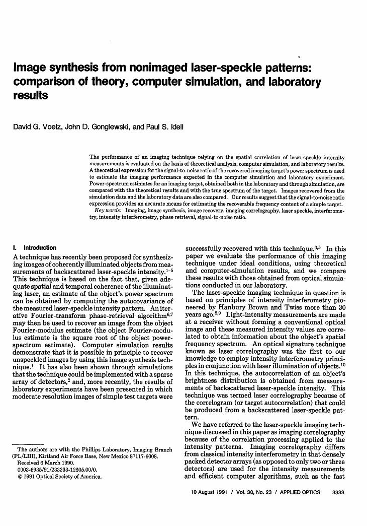
Fig. 1. Schematic diagram of the imaging correlography technique.
(a)
Fourier transform (as compared with analog multipliercircuits), are employed for the correlation process.Additionally, because only the object's power spec-trum can be determined from the intensity interferom-etry measurements directly, the iterative transformphase-retrieval algorithm is employed in imaging cor-relography to obtain the object's Fourier phase neededto recover images. In this way, imaging correlographyis an extension of both classical intensity interferome-try and the technique known as laser correlography, inwhich only object autocorrelations are generated.
A practical implementation of the imaging correlo-graphy technique is illustrated schematically in Fig. 1.The target is flood illuminated with coherent laserlight and the backscattered intensity is detected by a
(b)
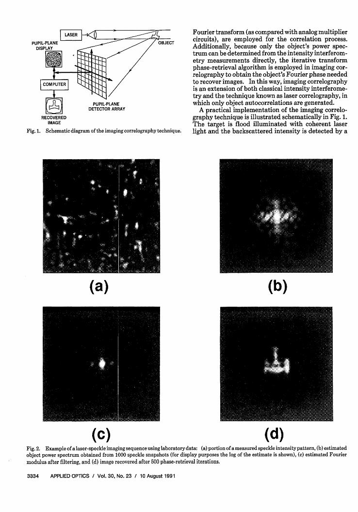
(C) (d)Fig. 2. Example of a laser-speckle imaging sequence using laboratory data: (a) portion of a measured speckle intensity pattern, (b) estimatedobject power spectrum obtained from 1000 speckle snapshots (for display purposes the log of the estimate is shown), (c) estimated Fourier
modulus after filtering, and (d) image recovered after 500 phase-retrieval iterations.
pupil-plane detector array. The intensity measure-ments are digitized and sent to a computer where theautocovariance of the intensity pattern is computed.As noted above, the autocovariance of the intensitypattern provides an estimate of the object's powerspectrum. For most practical imaging geometries, wefind that a single realization (snapshot) of speckleintensity yields a rather noisy estimate of the object'spower spectrum. Therefore in most cases a number ofindependent speckle snapshots of an object need to berecorded, processed, and averaged to form a power-spectrum estimate that is acceptable for recovering animage of the target. In practice independent specklepatterns can occur if the object rotates slightly or if theobject and measurement planes are displaced. Final-ly, the phase-retrieval algorithm is applied in the com-puter to the square root of the power-spectrum esti-mate (Fourier modulus) to recover the object phaseand therefore allow an image to be reconstructed.
An example of a typical correlography imaging se-quence using laboratory data is shown in Fig. 2. A 128X 128 pixel portion of a measured speckle snapshot isshown in Fig. 2(a), and the estimated object powerspectrum recovered from 1000 speckle snapshots isshown in Fig. 2(b) (for display purposes the log of theestimate is actually shown). Figure 2(c) shows theestimated object Fourier modulus obtained after aWiener-type filter has been applied to the data toreduce noise, and Fig. 2(d) shows the image recoveredafter 500 phase-retrieval iterations. For this image, arandom phase starting guess was used to initiate thephase-retrieval sequence. Note that the recoveredimage is unspeckled even though coherent illumina-tion was used. This, of course, is a result of the factthat the laser-speckle correlations formed in the imag-ing correlography processing provide, by means of theVan Cittert-Zernike theorem, an estimate of the Fou-rier coefficients of the (unspeckled) object brightnessfunction.
It can be shown that the sensitivity of a field ampli-tude interferometer, such as a Michelson interferome-ter, for recovering object spatial-frequency compo-nents is typically better than the sensitivity of anintensity interferometer.11"12 However, intensity in-terferometry techniques hold a few practical advan-tages over amplitude techniques. First, arrays of largedimensions can be more readily fabricated for intensi-ty interferometry techniques because optical path dif-ferences and mirror figure at the receiver are of minorconcern. Second, for Earth-based systems viewingobjects in space, wave-front phase aberrations owing tolow-altitude turbulence will have little effect on themeasured intensities, and only scintillation effects ow-ing to high-altitude turbulence are of concern. Per-haps the most serious limitation of the intensity inter-ferometer is that object phase is difficult to obtainfrom the intensity measurements. Higher-order in-tensity correlation techniques can be used to obtainobject phase,'3-'5 although in this case the signal-to-noise ratio (SNR) of the recovered phase values will beespecially poor. For imaging correlography, we take
advantage of object size and positivity constraints toretrieve the object phase with an iterative, Fienup-type Fourier-transform algorithm.
In this paper we include a review of the theory that isthe basis for the imaging correlography technique, andwe describe the computer-simulation approach, data-processing algorithms, and the laboratory optical sim-ulation setup. The results that we present in thispaper were obtained from a set of 1000 independentspeckle snapshots generated by computer simulationand a similar set of 1000 speckle snapshots collected inthe laboratory. Subsets of the simulation and labora-tory data were processed to yield object power-spec-trum estimates for various numbers of speckle snap-shots. We compare the recovered object-spectrumestimates with a theoretically derived expression forthe SNR of the power-spectrum estimate. We alsocompare (qualitatively) the images recovered from thesimulation and the laboratory data, and we discussdifferences between simulation and laboratory resultsthat begin to address some of the practical difficultiesin implementing the imaging correlography techniquewith real hardware.
11. Review of Theory
The theory on which imaging correlography is basedwas developed previously.",2 In this section we revisitthis work and add some discussion relevant to thecomputer simulation and laboratory implementationof imaging correlography. If an object with a diffusesurface is flood illuminated with laser light and theobject lies entirely within the coherence volume of thelaser beam (both spatially and temporally), then thebackscattered intensity will produce a fully developedspeckle pattern.16 In the far field, a single realizationof the observed speckle pattern, I(u), can be ex-pressed as the squared modulus of the Fourier trans-form of the complex field reflected at the object's sur-face:
In(U) = Il9fn(x)i 2, (1)
where indicates a Fourier transform and the reflect-ed object field, f(x), is given by
fj(x) = If0(x)1exp[i0,,(x)], (2)
where fo(x)I is the object's field amplitude reflectivityand k,(x) is the phase of the nth realization of thereflected field associated with the object's random sur-face height profile. The variable x represents a two-dimensional spatial coordinate in the object plane, andu represents a two-dimensional coordinate in the ob-servation plane.
It is known that from the average energy spectrum ofa laser-speckle intensity pattern one can obtain theautocorrelation function of the illuminated object'sbrightness distribution.' 5 Alternatively, one canequate the autocovariance of a laser-speckle intensitypattern to the power spectrum of the object's bright-ness distribution. The autocovariance of a specklepattern can be estimated from N independent realiza-tions of the pattern with the following expression:
C,(Au, N) = k E J P(u + Au)P(u)[In(u + Au) - 1'[lI(u) - fldu
= JJ P(U + AU)P(U) {k E [I(u + AU) -n=1
X [In(U) - II}d2U, (3)
where Aiu is a vector separation in the measurementplane and I is the (ensemble) mean intensity of thespeckle pattern. P(u) is the pupil function that de-fines the collecting aperture of the optical receiverused to observe each independent realization or snap-shot.
If we assume the backscattered field in the observa-tion plane is circular-complex Gaussian (which is validfor fully developed speckle patterns), then the momentfactoring theorem for circular-complex Gaussianfields'6 may be used to show that, in the limit as Napproaches infinity,
1 N
lim Z [In(u + Au) - I[In(u)-I = r(Au)2, (4)n=1
where P(Au) is the mutual coherence function of thespeckle field evaluated at points separated by Au.Equations (3) and (4) may then be combined to give
lim C,(Au, N) = OTF(Au)r(Au)J 2 , (5)N-
where OTF(Au) is the autocorrelation of the pupilfunction. By virtue of the Van Cittert-Zernike theo-rem, I(Au)12 is also equivalent to the power spectrumof the object's brightness distribution and Au can beconsidered a spatial-frequency variable. Thus, in thelimit N - -, the estimate C1(Au, N) yields the powerspectrum of the object's brightness distributionweighted by the function OTF(Au), which we refer toas the optical transfer function for the imaging correlo-graphy system.
In practice, the number of speckle snapshots N isalways finite, and we expect the quality of the estimateof the object's power spectrum to improve as N in-creases. This effect can be described in terms of aSNR of the intensity pattern autocovariance estimate.If we define the SNR to be the expected value of 0Idivided by the square root of the variance of Ci, andassume high light conditions (more than a few photonsper speckle lobe), the SNR as a function of Au and Nfor the estimator defined in Eq. (3) may be shown to beapproximately (see Appendix A)
where Ns is the number of speckles (or speckle lobes)contained in a single frame of speckle intensity, ,g(Au)is the complex coherence factor of the speckle fielddefined by pL(Au) = (Au) /, and OTF is the opticaltransfer function normalized by the pupil area. Wetypically assume the size of a speckle lobe to be \z/Wwhere X is the laser wavelength, z is the distance from
the target to the receiver, and W is the average linearwidth (or support) of the target. Thus the number ofspeckles in a single realization (or snapshot) is given by
N (WD)S (7)
where a square object of width Wand a square collect-ing aperture of dimension D have been assumed. It isemphasized that the noise inferred in Eq. (6) is due tothe classical statistical nature of the speckle patternsince photon counting and detector noise have beenignored in the derivation of Eq. (6). Equation (6) wasalso derived with assumptions that favor spatial fre-quencies in the midrange of the function OTF(Au).However, we have conducted simulations that suggestthat the expression may be accurate within a factor of 2for lower and higher spatial frequencies. It is appar-ent from Eq. (6) that the SNR of the recovered fre-quency components is proportional to the object'spower spectrum and the square root of the total num-ber of speckles collected. As a consequence, the quali-ty of our age estimate will depend on the size and shapeof the object scene as well as on the collecting apertureused.
Up to this point we have limited our discussion toour estimate of the object's power spectrum. Produc-ing an image from the correlation measurements, how-ever, requires that the Fourier phase of the object mustbe obtained (using phase retrieval) and combined withthe Fourier-modulus data. Thus, truly to characterizethe imaging performance of the imaging correlographytechnique, we must consider the effects of the phase-retrieval algorithm as a step in the image recoveryprocess. Our reliance on phase retrieval, however,introduces some practical difficulties that complicatethe image evaluation process.
First and foremost, predictions of the image qualityare hampered by the iterative and nonlinear nature ofthe phase-retrieval process itself. For example, thenonlinearity of the phase-retrieval process makes alinear systems-type description for image recovery ex-tremely cumbersome, if not impractical. To avoidsuch difficulties, and to tie imaging performance pre-dictions to our laboratory and simulation experience,we have chosen to characterize the imaging perfor-mance on the basis of the fidelity of the object's power-spectrum estimate. In doing so, we assume that thenature of the phase-retrieval process, if properly exe-cuted, is such that small errors in the Fourier-modulusestimate result in small errors in the recovered imageand hypothesize that the quality of the images formedfrom imaging correlography is, for the range of mea-surement conditions that we consider, entirely deter-mined by the fidelity of the power-spectrum estimate.We have found from extensive experience with com-puter simulations and laboratory data that this hy-pothesis is generally true, and we seek to demonstratethis relationship by considering some example cases inthis paper.
The second practical difficulty is derived from the
fact that, when phase retrieval is applied to Fourier-modulus data, the recovered image often contains arti-facts that have no counterpart in the original object(i.e., there is evidence of features not present in theoriginal object). Fienup and Wackerman have shownthat artifacts such as striping and twinning can beremoved if several images are recovered from differentstarting guesses and the results are combined in anappropriate way.7 However even if these techniquesare applied, one cannot be sure that the best imagepossible has been obtained from the available data,and Fienup's commonly used error metric6 cannotidentify the presence of low-level artifacts in the recov-ered images. We do not believe that the occurrence ofartifacts is a fundamental limitation of the phase-retrieval technique, since with enough patience, com-puter processing, and use of several image quality met-rics, one can usually obtain an image that is quitesimilar to the best possible image.
To avoid image artifacts and to speed up the phase-retrieval processing, we have used a rendering of theoriginal object (or truth object) as the starting guess inthe phase-retrieval processing. In this way, the phase-retrieval iteration begins at or near the optimum-im-age solution and diverges as the noisy (or incorrect)Fourier-modulus values are imposed on the image esti-mate. We have found that proceeding in this mannerproduces an image whose error metric value rapidlyconverges (in 10 iterations or so) to a value that is lessthan that obtained with any of a large number ofrandom starting image guesses. As one might expect,the image recovered in this way resembles a blurredversion of the original with no unexpected image arti-facts. We use this approach to obtain artifact-freeimages recovered from both computer simulations anddata collected in the laboratory.
111. Computer and Laboratory Simulation Approach
A. Computer Simulation
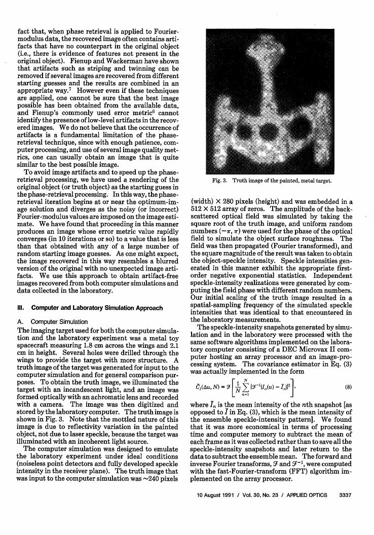
The imaging target used for both the computer simula-tion and the laboratory experiment was a metal toyspacecraft measuring 1.8 cm across the wings and 2.1cm in height. Several holes were drilled through thewings to provide the target with more structure. Atruth image of the target was generated for input to thecomputer simulation and for general comparison pur-poses. To obtain the truth image, we illuminated thetarget with an incandescent light, and an image wasformed optically with an achromatic lens and recordedwith a camera. The image was then digitized andstored by the laboratory computer. The truth image isshown in Fig. 3. Note that the mottled nature of thisimage is due to reflectivity variation in the paintedobject, not due to laser speckle, because the target wasilluminated with an incoherent light source.
The computer simulation was designed to emulatethe laboratory experiment under ideal conditions(noiseless point detectors and fully developed speckleintensity in the receiver plane). The truth image thatwas input to the computer simulation was -240 pixels
Fig. 3. Truth image of the painted, metal target.
(width) X 280 pixels (height) and was embedded in a512 X 512 array of zeros. The amplitude of the back-scattered optical field was simulated by taking thesquare root of the truth image, and uniform randomnumbers (--r, 7r) were used for the phase of the opticalfield to simulate the object surface roughness. Thefield was then propagated (Fourier transformed), andthe square magnitude of the result was taken to obtainthe object-speckle intensity. Speckle intensities gen-erated in this manner exhibit the appropriate first-order negative exponential statistics. Independentspeckle-intensity realizations were generated by com-puting the field phase with different random numbers.Our initial scaling of the truth image resulted in aspatial-sampling frequency of the simulated speckleintensities that was identical to that encountered inthe laboratory measurements.
The speckle-intensity snapshots generated by simu-lation and in the laboratory were processed with thesame software algorithms implemented on the labora-tory computer consisting of a DEC Microvax II com-puter hosting an array processor and an image-pro-cessing system. The covariance estimator in Eq. (3)was actually implemented in the form
C1(Au, N) = 5 -[k 1 I '{In(u) - ] (8)
where I, is the mean intensity of the nth snapshot [asopposed to I in Eq. (3), which is the mean intensity ofthe ensemble speckle-intensity pattern]. We foundthat it was more economical in terms of processingtime and computer memory to subtract the mean ofeach frame as it was collected rather than to save all thespeckle-intensity snapshots and later return to thedata to subtract the ensemble mean. The forward andinverse Fourier transforms, 5r and gr-l, were computedwith the fast-Fourier-transform (FFT) algorithm im-plemented on the array processor.
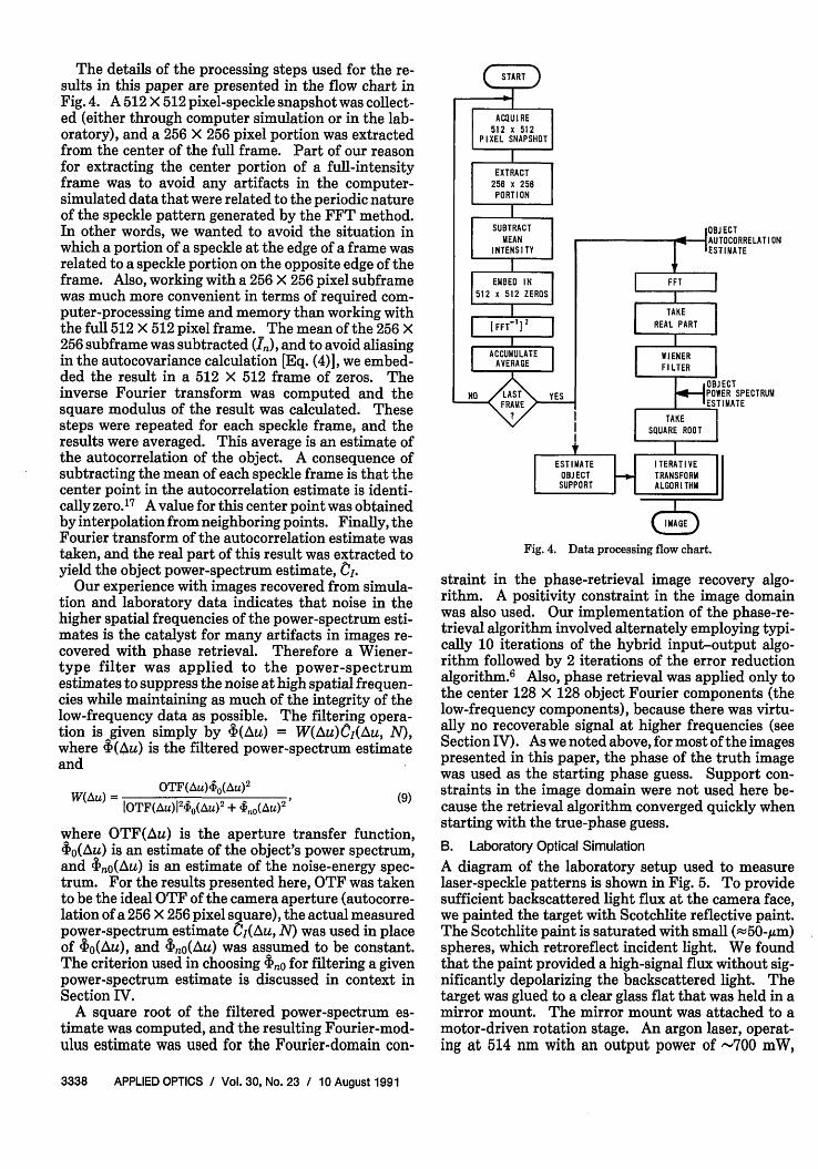
The details of the processing steps used for the re-sults in this paper are presented in the flow chart inFig. 4. A 512 X 512 pixel-speckle snapshot was collect-ed (either through computer simulation or in the lab-oratory), and a 256 X 256 pixel portion was extractedfrom the center of the full frame. Part of our reasonfor extracting the center portion of a full-intensityframe was to avoid any artifacts in the computer-simulated data that were related to the periodic natureof the speckle pattern generated by the FFT method.In other words, we wanted to avoid the situation inwhich a portion of a speckle at the edge of a frame wasrelated to a speckle portion on the opposite edge of theframe. Also, working with a 256 X 256 pixel subframewas much more convenient in terms of required com-puter-processing time and memory than working withthe full 512 X 512 pixel frame. The mean of the 256 X256 subframe was subtracted (I), and to avoid aliasingin the autocovariance calculation [Eq. (4)], we embed-ded the result in a 512 X 512 frame of zeros. Theinverse Fourier transform was computed and thesquare modulus of the result was calculated. Thesesteps were repeated for each speckle frame, and theresults were averaged. This average is an estimate ofthe autocorrelation of the object. A consequence ofsubtracting the mean of each speckle frame is that thecenter point in the autocorrelation estimate is identi-cally zero.'7 A value for this center point was obtainedby interpolation from neighboring points. Finally, theFourier transform of the autocorrelation estimate wastaken, and the real part of this result was extracted toyield the object power-spectrum estimate, CI.
Our experience with images recovered from simula-tion and laboratory data indicates that noise in thehigher spatial frequencies of the power-spectrum esti-mates is the catalyst for many artifacts in images re-covered with phase retrieval. Therefore a Wiener-type filter was applied to the power-spectrumestimates to suppress the noise at high spatial frequen-cies while maintaining as much of the integrity of thelow-frequency data as possible. The filtering opera-tion is given simply by -$(Au) = W(Au)01(Au, N),where $(Au) is the filtered power-spectrum estimateand
W(A) OTF(Au)bO(Au) 2 (9)-10TF(Au)J
2.j0(AU)2 + (%0(AU)2
where OTF(Au) is the aperture transfer function,$O(Au) is an estimate of the object's power spectrum,and $n(Au) is an estimate of the noise-energy spec-trum. For the results presented here, OTF was takento be the ideal OTF of the camera aperture (autocorre-lation of a 256 X 256 pixel square), the actual measuredpower-spectrum estimate I(Au, N) was used in placeof $o(Au), and $nO(Au) was assumed to be constant.The criterion used in choosing 'I'nO for filtering a givenpower-spectrum estimate is discussed in context inSection IV.
A square root of the filtered power-spectrum es-timate was computed, and the resulting Fourier-mod-ulus estimate was used for the Fourier-domain con-
Fig. 4. Data processing flow chart.
straint in the phase-retrieval image recovery algo-rithm. A positivity constraint in the image domainwas also used. Our implementation of the phase-re-trieval algorithm involved alternately employing typi-cally 10 iterations of the hybrid input-output algo-rithm followed by 2 iterations of the error reductionalgorithm.6 Also, phase retrieval was applied only tothe center 128 X 128 object Fourier components (thelow-frequency components), because there was virtu-ally no recoverable signal at higher frequencies (seeSection IV). As we noted above, for most of the imagespresented in this paper, the phase of the truth imagewas used as the starting phase guess. Support con-straints in the image domain were not used here be-cause the retrieval algorithm converged quickly whenstarting with the true-phase guess.
B. Laboratory Optical Simulation
A diagram of the laboratory setup used to measurelaser-speckle patterns is shown in Fig. 5. To providesufficient backscattered light flux at the camera face,we painted the target with Scotchlite reflective paint.The Scotchlite paint is saturated with small (-50-,gm)spheres, which retroreflect incident light. We foundthat the paint provided a high-signal flux without sig-nificantly depolarizing the backscattered light. Thetarget was glued to a clear glass flat that was held in amirror mount. The mirror mount was attached to amotor-driven rotation stage. An argon laser, operat-ing at 514 nm with an output power of -700 mW,
produced a beam that was expanded to illuminate thetarget uniformly. The scattered (but nonimaged) la-ser-speckle intensity was recorded with a 512 X 512pixel charge-injection device camera (7.7-mm-squareaperture). The camera was operated without a lens torecord the laser-speckle intensity pattern falling uponthe camera's faceplate. The camera was positioned sothe detector plane was 2.5 m from the target. If weagain assume the size of a speckle lobe to be Xz/W [Eq.(8)], then the number of detector elements that sam-pled each speckle lobe was approximately
(AZ ) = 18.3 detectors/speckle lobe,
where the center-to-center spacing of each detectorelement d was 15,um, the average object width W was-2 mm, the camera-target distance z was 2.5 m, andthe laser wavelength X was 514 nm. Independent real-izations of the detected speckle pattern were obtainedby rotating the object with the mirror mount-steppermotor arrangement. Data frames acquired by thecamera were digitized and stored by the laboratorycomputer. The speckle snapshots were then pro-cessed as described in Subsection III.A.
Ideally, before the speckle snapshots are processedthe measured speckle intensities should be correctedfor sensor artifacts, such as camera modulation trans-fer function and nonlinear intensity response. For ourexperiment, the charge-injection device camera's mod-ular transfer function was measured with an edge-response technique' 8 to be close to 100% out to a spatialfrequency of 20 cycles/mm, whereas the highest spatialfrequency in the speckle pattern at the camera sensorwas calculated to be just 16 cycles/mm. In addition,the camera response was measured in the laboratory tobe linear over the intensity ranges encountered in theexperiment. Therefore correction of these camera ar-tifacts in the laboratory data was deemed unnecessary.
IV. Comparison of Theory, Laboratory, and SimulationResults
When analyzing and comparing the simulation andlaboratory data, we found it helpful initially to consid-er the object power-spectrum estimate rather than thefully reconstructed image. For our laboratory setup,
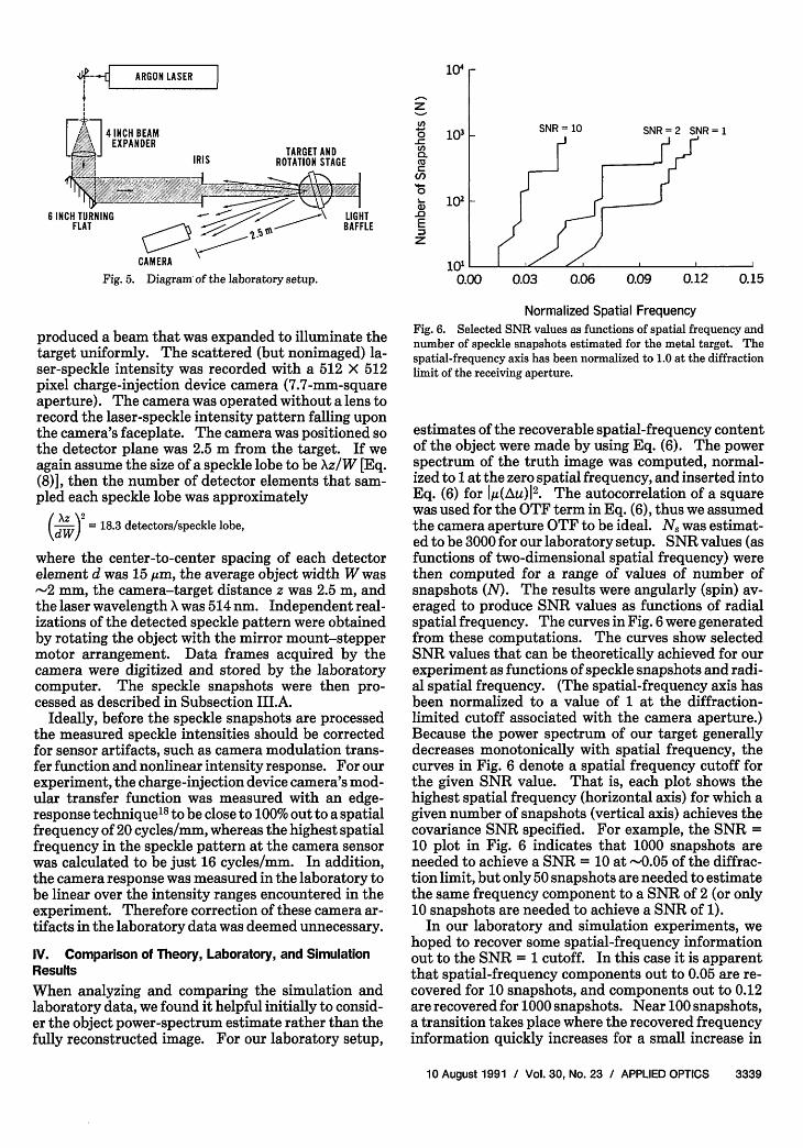
Normalized Spatial FrequencyFig. 6. Selected SNR values as functions of spatial frequency andnumber of speckle snapshots estimated for the metal target. Thespatial-frequency axis has been normalized to 1.0 at the diffractionlimit of the receiving aperture.
estimates of the recoverable spatial-frequency contentof the object were made by using Eq. (6). The powerspectrum of the truth image was computed, normal-ized to I at the zero spatial frequency, and inserted intoEq. (6) for IM(Au)J2. The autocorrelation of a squarewas used for the OTF term in Eq. (6), thus we assumedthe camera aperture OTF to be ideal. N was estimat-ed to be 3000 for our laboratory setup. SNR values (asfunctions of two-dimensional spatial frequency) werethen computed for a range of values of number ofsnapshots (N). The results were angularly (spin) av-eraged to produce SNR values as functions of radialspatial frequency. The curves in Fig. 6 were generatedfrom these computations. The curves show selectedSNR values that can be theoretically achieved for ourexperiment as functions of speckle snapshots and radi-al spatial frequency. (The spatial-frequency axis hasbeen normalized to a value of 1 at the diffraction-limited cutoff associated with the camera aperture.)Because the power spectrum of our target generallydecreases monotonically with spatial frequency, thecurves in Fig. 6 denote a spatial frequency cutoff forthe given SNR value. That is, each plot shows thehighest spatial frequency (horizontal axis) for which agiven number of snapshots (vertical axis) achieves thecovariance SNR specified. For example, the SNR =10 plot in Fig. 6 indicates that 1000 snapshots areneeded to achieve a SNR = 10 at -0.05 of the diffrac-tion limit, but only 50 snapshots are needed to estimatethe same frequency component to a SNR of 2 (or only10 snapshots are needed to achieve a SNR of 1).
In our laboratory and simulation experiments, wehoped to recover some spatial-frequency informationout to the SNR = 1 cutoff. In this case it is apparentthat spatial-frequency components out to 0.05 are re-covered for 10 snapshots, and components out to 0.12are recovered for 1000 snapshots. Near 100 snapshots,a transition takes place where the recovered frequencyinformation quickly increases for a small increase in
RADIAL AVERAGE POWER SPECTRUM ESTIMATES -SIMULATION RESULTS
.% N= 10 --
IN = 100SNR = 1
10-4F SN= 10SNR = 1
10-5 L_.0.00
a)LU
a)N
E0zi
SN = 1 (TRUTH x
0.05 0.10 0.15 0.20 0.25
10-1
10-2
10-3
10-4
lo-5 L0.00
RADIAL AVERAGE POWER SPECTRUM ESTIMATES -LABORATORY RESULTS
0.05 0.10 0.15 0.20 0.25
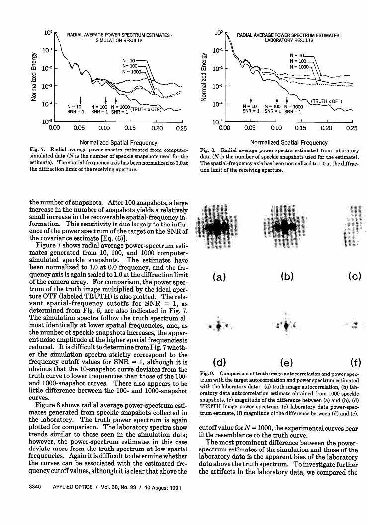
Normalized Spatial FrequencyFig. 7. Radial average power spectra estimated from computer-simulated data (N is the number of speckle snapshots used for theestimate). The spatial-frequency axis has been normalized to 1.0 atthe diffraction limit of the receiving aperture.
the number of snapshots. After 100 snapshots, a largeincrease in the number of snapshots yields a relativelysmall increase in the recoverable spatial-frequency in-formation. This sensitivity is due largely to the influ-ence of the power spectrum of the target on the SNR ofthe covariance estimate [Eq. (6)].
Figure 7 shows radial average power-spectrum esti-mates generated from 10, 100, and 1000 computer-simulated speckle snapshots. The estimates havebeen normalized to 1.0 at 0.0 frequency, and the fre-quency axis is again scaled to 1.0 at the diffraction limitof the camera array. For comparison, the power spec-trum of the truth image multiplied by the ideal aper-ture OTF (labeled TRUTH) is also plotted. The rele-vant spatial-frequency cutoffs for SNR = 1, asdetermined from Fig. 6, are also indicated in Fig. 7.The simulation spectra follow the truth spectrum al-most identically at lower spatial frequencies, and, asthe number of speckle snapshots increases, the appar-ent noise amplitude at the higher spatial frequencies isreduced. It is difficult to determine from Fig. 7 wheth-er the simulation spectra strictly correspond to thefrequency cutoff values for SNR = 1, although it isobvious that the 10-snapshot curve deviates from thetruth curve to lower frequencies than those of the 100-and 1000-snapshot curves. There also appears to belittle difference between the 100- and 1000-snapshotcurves.
Figure 8 shows radial average power-spectrum esti-mates generated from speckle snapshots collected inthe laboratory. The truth power spectrum is againplotted for comparison. The laboratory spectra showtrends similar to those seen in the simulation data;however, the power-spectrum estimates in this casedeviate more from the truth spectrum at low spatialfrequencies. Again it is difficult to determine whetherthe curves can be associated with the estimated fre-quency cutoff values, although it is clear that above the
Normalized Spatial FrequencyFig. 8. Radial average power spectra estimated from laboratorydata (N is the number of speckle snapshots used for the estimate).The spatial-frequency axis has been normalized to 1.0 at the diffrac-tion limit of the receiving aperture.
(a)
... ..
(b) (c)
(d) (e) (f)Fig. 9. Comparison of truth image autocorrelation and power spec-trum with the target autocorrelation and power spectrum estimatedwith the laboratory data: (a) truth image autocorrelation, (b) lab-oratory data autocorrelation estimate obtained from 1000 specklesnapshots, (c) magnitude of the difference between (a) and (b), (d)TRUTH image power spectrum, (e) laboratory data power-spec-trum estimate, (f) magnitude of the difference between (d) and (e).
cutoff value for N = 1000, the experimental curves bearlittle resemblance to the truth curve.
The most prominent difference between the power-spectrum estimates of the simulation and those of thelaboratory data is the apparent bias of the laboratorydata above the truth spectrum. To investigate furtherthe artifacts in the laboratory data, we compared the
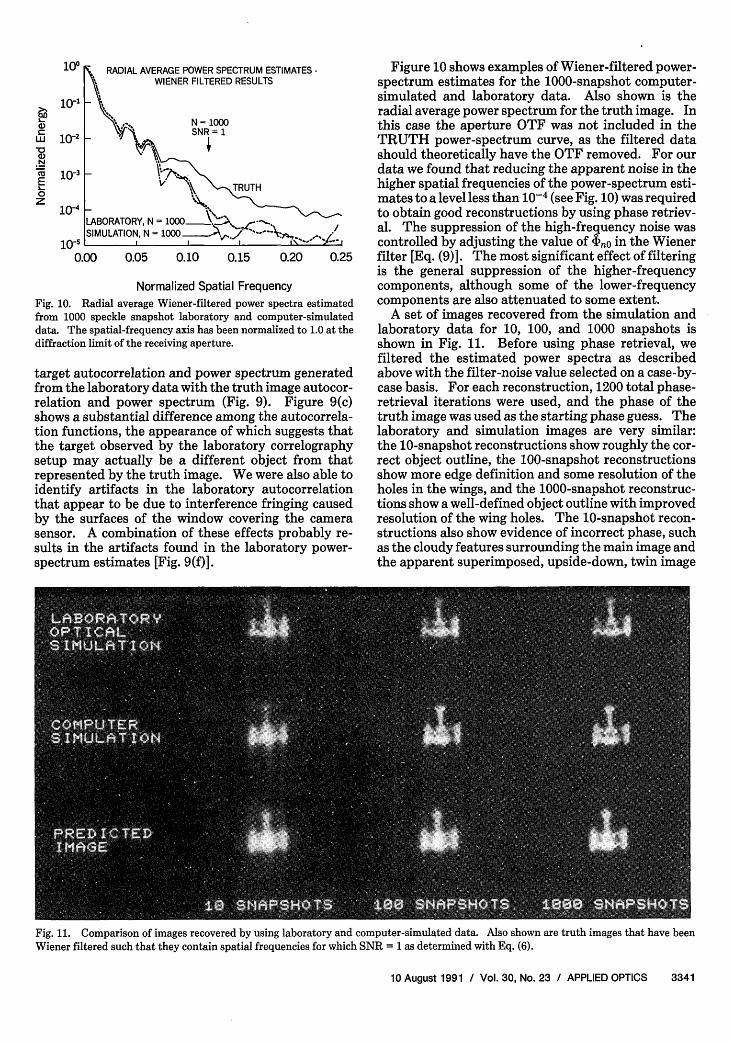
Fig. 10. Radial average Wifrom 1000 speckle snapshotdata. The spatial-frequencydiffraction limit of the receiv
target autocorrelation afrom the laboratory datrelation and power spishows a substantial difftion functions, the appthe target observed bysetup may actually berepresented by the trut]identify artifacts in tithat appear to be due tby the surfaces of thesensor. A combinationsuits in the artifacts fospectrum estimates [Fii
E POWER SPECTRUM ESTIMATES - Figure 10 shows examples of Wiener-filtered power-NER FILTERED RESULTS spectrum estimates for the 1000-snapshot computer-
simulated and laboratory data. Also shown is theradial average power spectrum for the truth image. In
N = 10 this case the aperture OTF was not included in theSNR = 1 TRUTH power-spectrum curve, as the filtered data
should theoretically have the OTF removed. For ourdata we found that reducing the apparent noise in the
TRUTH higher spatial frequencies of the power-spectrum esti-mates to a level less than 10-4 (see Fig. 10) was required
00 to obtain good reconstructions by using phase retriev-00>2:: -. :z, X al. The suppression of the high-frequency noise was
I " ;; 4-- i controlled by adjusting the value of PnO in the Wiener0.10 0.15 0.20 0.25 filter [Eq. (9)]. The most significant effect of filtering
is the general suppression of the higher-frequencyized Spatial Frequency components, although some of the lower-frequencymer-filtered power spectra estimated components are also attenuated to some extent.laboratory and computer-simulated A set of images recovered from the simulation and
axis has been normalized to 1.0 at the laboratory data for 10, 100, and 1000 snapshots isng aperture. shown in Fig. 11. Before using phase retrieval, we
filtered the estimated power spectra as describedand power spectrum generated above with the filter-noise value selected on a case-by-i with the truth image autocor- case basis. For each reconstruction, 1200 total phase-actrum (Fig. 9). Figure 9(c) retrieval iterations were used, and the phase of theerence among the autocorrela- truth image was used as the starting phase guess. Theearance of which suggests that laboratory and simulation images are very similar:the laboratory correlography the 10-snapshot reconstructions show roughly the cor-a different object from that rect object outline, the 100-snapshot reconstructions
[h image. We were also able to show more edge definition and some resolution of theie laboratory autocorrelation holes in the wings, and the 1000-snapshot reconstruc-o interference fringing caused tions show a well-defined object outline with improvedwindow covering the camera resolution of the wing holes. The 10-snapshot recon-n of these effects probably re- structions also show evidence of incorrect phase, suchund in the laboratory power- as the cloudy features surrounding the main image andg. 9(f)]. the apparent superimposed, upside-down, twin image
Fig. 11. Comparison of images recovered by using laboratory and computer-simulated data. Also shown are truth images that have beenWiener filtered such that they contain spatial frequencies for which SNR = 1 as determined with Eq. (6).
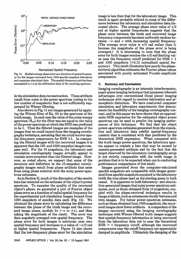
RADIAL AVERAGE PHASE ERROR image is less than that for the laboratory image. Thisresult is again probably related to some. of the differ-
LABORATORY ences between the laboratory and simulation data dis-LABORATORY C a m ..... - cussed above. The average phase error value of 7r/2
.-.. B y. ,- - rad at higher spatial frequencies suggests that thephase error between the truth and recovered imagefrequency components becomes uniformly random be-
SIMULATION tween -7r and r with increasing spatial frequency.(The average error value is 7r/2 rad rather than 0,because the magnitude of the phase error is beingaveraged.) It is interesting to note that the phaseerror for both images reaches the 7r/2-rad limiting val-
; , .. ue near the frequency cutoff predicted for SNR = 10.05 0.10 0.15 0.20 0.25 and 1000 snapshots (0.12 normalized spatial fre-
quency). This result illustrates how poorly the phase-Normalized Spatial Frequency retrieval algorithm estimates the Fourier-phase values
Fig. 12. Radial average phase error as a function of spatial frequen-cy for the images recovered from 1000-speckle snapshot laboratoryand computer-simulated data. The spatial-frequency axis has beennormalized to 1.0 at the diffraction limit of the receiving aperture.
in the simulation data reconstruction. These artifactsresult from noise in the power spectrum (owing to thelow number of snapshots) that is not sufficiently sup-pressed by Wiener filtering.
Also shown in Fig. I1 are images generated by apply-ing the Wiener filter of Eq. (9) to the spectrum of thetruth image. In each case the value ofthe noise-energyspectrum (nO) for the filter was set equal to the valueof the power spectrum at which the SNR was predictedto be 1. Thus the filtered images are examples of theimages that we could expect from the imaging correlo-graphy technique, assuming that we could recover spa-tial-frequency components for SNR >1. In compar-ing the filtered images with the recovered images it isapparent that the 100- and 1000-snapshot images com-pare well. For the 10 snapshots, the laboratory andsimulation correlography images actually appear tocontain more structure than the filtered image. How-ever, as noted above, we suspect that some of thestructure and definition in the 10-snapshot correlo-graphy images result from phase artifacts that arisefrom using phase retrieval with the noisy power-spec-trum estimates.
As in Section II, much of the discussion of the resultshere has centered on the estimate of the object's powerspectrum. To examine the quality of the recoveredobject's phase, we generated a plot of Fourier objectphase error as a function of radial spatial frequency forthe experimental and simulation images formed from1000 snapshots of speckle data each (Fig. 12). Weobtained the phase error by calculating the differencebetween the phase of the truth image and the recov-ered image phase, modulo 2r (-7r to +r), and thentaking the magnitude of the result. The error wasthen angularly averaged over spatial frequency. Thephase error for both images is minimum near zerospatial frequency and increases to a value of -7r/2 radat higher spatial frequencies. Figure 12 also showsthat the low-frequency phase error for the simulation
associated with poorly estimated tourier-amplitudecomponents.
V. Summary and Conclusions
Imaging correlography is an intensity interferometry,pupil-plane imaging technique that possesses inherentadvantages over conventional (focal plane) imagingtechniques with regard to receiver fabrication and at-mospheric distortion. We have conducted computersimulation and laboratory experiments that demon-strate the feasibility of the imaging correlography con-cept, and in this paper we have shown that an approxi-mate SNR expression for the estimated object powerspectrum can be used to predict the imaging perfor-mance of this technique. We find that the objectpower-spectrum estimates generated from the simula-tion and laboratory data exhibit spatial-frequencycontent that is consistent with that predicted by thetheoretical SNR expression. When compared withthe truth image power spectrum, the laboratory spec-tra appear to contain a bias that may be caused bycamera-generated artifacts and by the fact that thetarget observed by the laboratory correlography setupis not strictly comparable with the truth image (aproblem that is to be expected when one is conductingperformance comparisons of this kind).
Images generated from the computer-simulatedspeckle snapshots are comparable with images gener-ated from speckle snapshots acquired in the laboratory(with the true phase used as the starting guess in bothcases). It is apparent in both laboratory- and simula-tion-generated images that noisy power-spectrum esti-mates, such as those obtained from 10 snapshots, cou-pled with the phase-retrieval technique results inimage artifacts, such as extraneous cloudy features andtwin images. For better power-spectrum estimates,such as those obtained from 1000 snapshots, the recov-ered images show fewer artifacts. A comparison of theimages recovered using the imaging correlographytechnique with Wiener-filtered truth images suggeststhat spatial-frequency information is being recoveredfrom the laboratory data out to near the theoreticalSNR = 1 frequency cutoff, although the recoveredcomponents near the cutoff frequency are appreciablydamped in amplitude. Ultimately the damping of the
spatial-frequency components is associated with theWiener filter that is applied to reduce the noise ampli-tude in the power-spectrum estimates.
We found that our ability to estimate the object'sFourier-phase components by using the phase-retriev-al algorithm was a strong function of the quality of theestimated Fourier-amplitude components, although inthis paper we did not attempt to quantify this relation-ship. It may be possible to quantify the phase errorassociated with phase retrieval in terms of a wave-fronterror, which can in turn be related to image quality.
Appendix A
In this appendix we derive an approximate expressionfor the SNR of the covariance estimate used in thispaper. The analysis that we present is similar to thatfound in SNR studies investigating other speckle-in-tensity correlation estimators. 0 92 0 The expressionderived in this appendix and presented as Eq. (6) in themain body of the paper is valid under high light condi-tions-that is, when the object is illuminated withsufficient laser power that the performance of the esti-mator is limited by the random intensity fluctuationsassociated with the laser-speckle process and not byphoton-counting considerations or other noise pro-cesses. Additionally, we ignore certain (higher-order)cross terms in the calculation of the variance of thespeckle-intensity covariance estimator. Althoughthis approximation greatly simplifies the calculation,it also allows one to quantify easily the extent to whicha redundant collecting aperture improves the perfor-mance of the speckle covariance estimator.
The SNR is defined by the ensemble mean of thespeckle-intensity covariance divided by the squareroot of the ensemble variance of the covariance esti-mate:
where Au is the vector separation of detectors in thepupil plane, E is the expectation operation, and Var isthe variance, and C1(Au, 1) is the single-snapshot co-variance estimate given by Eq. (3) with N = 1:
Hence, assuming that the N speckle snapshots used toestimate the intensity covariance are drawn from anergodic ensemble, the SNR of the N-snapshot, redun-dant-aperture estimator [Eq. (3)] is just the squareroot of N times the SNR of the single-snapshot estima-tor [Eq. (A2)].
The expected value of the covariance estimate maybe computed by applying the expectation operatordirectly to Eq. (A2). Assuming that the laser-speckleprocess is ergodic, the result of this operation is givenin Eq. (5):
Equation (A5) shows that the variance of the redun-dant-aperture covariance estimator C1(Au, 1) may becomputed through a four-dimensional integral overthe covariance Kc of the two-point covariance estima-tor cJ. This integral accumulates [for all possible val-ues of x and x' in the collecting aperture P(x)] the noisevariance contributions associated with two pairs ofintensity samples separated by displacement Au.
Assuming that the contributions of the covarianceKC to the integral in Eq. (A5) are negligible except forregions Ix - x'1 2 < A, (where A, is the approximate areaof a laser-speckle correlation cell), we may approxi-mate the covariance of the speckle-intensity covari-ance by2l
K,(Au; x, x') Var c1 (Au)Asb(x -x'), (A8)
where 5(x - x') is a two-dimensional Dirac delta func-tion and
We achieved the last equality in Eq. (A9) (after somearithmetic) by expanding the indicated products in thefirst line, using Eq. (A7), and then applying the mo-ment factoring theorem for circular-complex Gaussianrandom variables.'2 Above, ,u(Ax) = r(Ax)/I is thecomplex coherence factor of the speckle field, and Ax =x - x' is the vector displacement between x and x'.Note that, since the speckle field is statistically homo-geneous, the complex coherence factor can be ex-pressed as a function of only one (vector) coordinateAx. (The covariance KC can, therefore, always be ex-pressed as a function of only two vector coordinates,e.g., Ax and Au.)
Substituting the approximate covariance (A8) intothe integral in Eq. (A5) yields
Var 0j(Au, 1) Var c(Au)A.OTF(Au), (A10)
where A, is again the effective area of a laser-specklelobe and Var c1(Au) is given by Eq. (A9). Further
substituting relation (A10) together with the expres-sion for the mean [Eq. (A3)] into Eq. (Al) gives thedesired approximate expression for the SNR of thecovariance estimator used in this paper:
is the effective number of speckles contained in thereceiving aperture given approximately by Eq. (7) inthe main text and OTF(Au) = OTF(Au)/Ap is the OTFfunction normalized by the area of the collecting aper-ture. Equation (A12) is the same as Eq. (6), which wasto be shown.
In closing, we note that approximation (A8) for thecovariance estimate cj(Au) [cf. Eq. (A7)] allows us toexpress the redundant-aperture SNR conveniently asan elemental SNR given by Ecj(Au)/[Var c(Au)]/ 2
[expressed in the first term of either relation (All) orEq. (A12)] times a redundancy factor, N N OTF(Au)'/2
This redundancy factor is equal to the square root ofthe effective number of the independent speckle-in-tensity sample pairs collected and processed to formthe imaging correlography covariance estimate.Above, N is the number of independent redundant-aperture snapshots processed, NS is the effective num-ber of laser-speckle lobes contained in the collectingaperture, and OTF(Au) is the normalized OTF, whichspecifies the spatial-frequency coverage of the collect-ing aperture.
The authors thank Bob Pierson for developing thelaboratory data acquisition software, Brian Kelly andArthur Webster for helping with data collection andprocessing, and David Dayton for recovering the im-ages using phase retrieval.
References
1. P. S. Idell, J. R. Fienup, and R. S. Goodman, "Image Synthesisfrom Nonimaged Laser-Speckle Patterns," Opt. Lett. 12, 858-860 (1987).
2. J. R. Fienup and P. S. Idell, "Imaging Correlography with SparseArrays of Detectors," Opt. Eng., 27, 778-784 (1988).
3. P. S. Idell, J. D. Gonglewski, D. G. Voelz, and J. Knopp, "ImageSynthesis from Nonimaged Laser-Speckle Patterns: Experi-mental Verification," Opt. Lett. 14, 154-156 (1989).
4. P. D. Henshaw and D. E. B. Lees, "Electronically Agile MultipleAperture Imager Receiver," Opt. Eng. 27, 793-800 (1988).
5. M. Nieto-Vesperinas, M. J. Perez-Ilzarbe, and R. Navarro, "Ob-ject Reconstruction from Experimental Far-Field Data UsingPhase Retrieval Algorithms," in Signal Recovery and SynthesisIII, Vol.15 of OSA 1989 Technical Digest Series (Optical Societyof America, Washington, D.C., 1989), pp. 146-149.
6. J. R. Fienup, "Phase Retrieval Algorithms: A Comparison,"Appl. Opt. 21, 2758-2769 (1982).
7. J. R. Fienup and C. C. Wackerman, "Phase Retrieval StagnationProblems and Solutions," J. Opt. Soc. Am. A 3, 1897-1907(1986).
8. R. Hanbury Brown and R. Q. Twiss, "A Test of a New Type ofStellar Interferometer on Sirius," Nature (London) 178, 1046-1048 (1956).
9. R. Hanbury Brown, The Intensity Interferometer (Taylor &Francis, London, 1974).
10. M. Elbaum, M. King, and M. Greenebaum, Laser Correlo-graphy: Transmission of High-Resolution Object SignaturesThrough the Turbulent Atmosphere, Tech. Rep. T-1/306-3-11(Riverside Research Institute, New York, 1974).
11. R. Q. Twiss, "Applications of Intensity Interferometry in Phys-ics and Astronomy," Opt. Acta 16, 423-451 (1969).
12. J. W. Goodman, Statistical Optics (Wiley, New York, 1985).13. T. Sato, S. Wadaka, J. Yamamoto, and J. Ishii, "Imaging System
Using an Intensity Triple Correlator," Appl. Opt. 17, 2047-2052(1978).
14. A. S. Marathay, "Phase Function of Spatial Coherence fromMultiple Intensity Correlations," in Advanced Technology Op-tical Telescopes III, L. D. Barr, ed., Proc. Soc. Photo-Opt.Instrum. Eng. 628, 273-276 (1986).
15. A. S. Marathay, Y. Hu, and P. S. Idell, "Object ReconstructionUsing Third and Fourth Order Intensity Correlations," present-ed at the Workshop On Higher-Order Spectral Analysis, Vail,Colo., 1989.
16. L. I. Goldfischer, "Autocorrelation Function and Power SpectralDensity of Laser-Produced Speckle Patterns," J. Opt. Soc. Am.55, 247-253 (1965).
17. K.-S. Kim and D. Caballero, "Derivation and Simulation of anImaging Correlography Algorithm: A Modification of the Idell-Fienup Algorithm," in Digital Image Recovery and Synthesis,P. S. Idell, ed., Proc. Soc. Photo-Opt. Instrum. Eng. 828,153-156(1987).
18. L. Fang and H. J. Tiziani, "A New Method for Determining theModulation-Transfer Function from Edge Traces," Optik 74,17-21 (1986).
19. K. A. O'Donnell, "Time-Varying Speckle Phenomena in Astro-nomical Imaging and in Laser Scattering," Ph.D. dissertation(University of Rochester, Rochester, N.Y., 1983).
20. J. C. Marron, "Accuracy of Fourier-Magnitude Estimation fromSpeckle Intensity Correlation," J. Opt. Soc. Am. A 5, 864-870(1988).
21. The assumption leading to condition (A8) ignores certain dou-ble-frequency effects that result in terms whose magnitudes aresmaller than the lil(Au)12 term in Eq. (A9) but in total may belarger than the ly(Au)14 term. For objects withsignificantdetail(such as that used in this paper), the IU(Au)12 term makes aninsignificant contribution to the overall SNR expression [cf. Eq.(A12)] at detector separations Au more than a few specklewidths. Hence the approximation leading to condition (A8)would seem justified for our experimental work.