Geophysical Journal International Geophys. J. Int. (2016) 204, 1332–1341 doi: 10.1093/gji/ggv511 GJI Seismology Imaging near-surface heterogeneities by natural migration of backscattered surface waves Abdullah AlTheyab, 1 Fan-Chi Lin 2 and Gerard T. Schuster 1 1 Department of Earth Science and Engineering, King Abdullah University of Science and Technology (KAUST), Thuwal 23955-6900, Saudi Arabia. E-mail: [email protected]2 Department of Geology and Geophysics, University of Utah, 271 Frederick Albert Sutton Building, Salt Lake City, UT 84112, USA Accepted 2015 November 25. Received 2015 September 16; in original form 2015 March 1 SUMMARY We present a migration method that does not require a velocity model to migrate backscattered surface waves to their projected locations on the surface. This migration method, denoted as natural migration, uses recorded Green’s functions along the surface instead of simulated Green’s functions. The key assumptions are that the scattering bodies are within the depth interrogated by the surface waves, and the Green’s functions are recorded with dense receiver sampling along the free surface. This natural migration takes into account all orders of multi- ples, mode conversions and non-linear effects of surface waves in the data. The natural imaging formulae are derived for both active source and ambient-noise data, and computer simulations show that natural migration can effectively image near-surface heterogeneities with typical ambient-noise sources and geophone distributions. Key words: Interferometry; Surface waves and free oscillations; Wave scattering and diffraction. 1 INTRODUCTION Backscattered surface waves can be imaged for the near-surface het- erogeneities (Snieder 1986). The typical strategy is to (1) linearize the relation between the scattered data d and the model perturbation m (i.e. heterogeneities map) under the Born approximation d = Lm, and then (2) find the approximate solution by either an iterative opti- mization method (Riyanti 2005; Campman & Riyanti 2007; Kaslilar 2007) or by applying the adjoint (Snieder 1986; Blonk et al. 1995; Campman et al. 2005; Yu et al. 2014) of the modeling operator L † to the scattered data d to get the migration image m mig = L † d. In all cases, the two key assumptions are that the velocity model (typically, just the smooth component of the surface wave veloc- ity distribution) is known and the weak-scattering approximation is invoked. For many practical applications, the background velocity model is assumed to be a layered medium. This methodology has found a growing number of uses in earthquake, exploration and en- gineering seismology (Snieder 1986; Blonk et al. 1995; Wijk 2003; Campman et al. 2005; Riyanti 2005; Campman & Riyanti 2007; Kaslilar 2007). There are two significant limitations with the above surface wave inversion methods: the Born approximation is invalid if there are strong velocity contrasts and the wavefields in complex regions of Earth cannot be accurately modelled without prior knowledge of the elastic parameters of Earth. In either case, the resulting image can contain significant errors. To eliminate these problems, we present a surface wave imaging method named natural migration (Schuster 2002; Brandsberg-Dahl et al. 2007; Sinha et al. 2009; Xiao & Schuster 2009; Hanafy & Schuster 2014) that does not require the Born approximation or the need to know the velocity model. Instead of computing the Green’s functions with an assumed background velocity model, we estimate the actual Green’s functions G(x g |x s ) of the earth at the geophone locations x g for either an active point source at x s , or a virtual point source at x s computed by cross- correlation and stacking of ambient-noise records. These estimated Green’s functions contain all of the effects of scattering, anisotropy and higher order modes in the data eliminating the need for compute- intensive elastic modeling operations (Schuster 2002). The Green’s functions are then used to create the exact modeling operator L that emulates the data, so there is no need to know the velocity model to find m mig = L † d. However, the trial image points are restricted to be at the surface, so the migration image provides the scatterer distributions projected from depth to their surface locations. The limitation is that the sampling of the migration image depends on the density of receiver arrays along the free surface. This limitation is mitigated by the recent availability of dense seismic arrays, such as USArray and the Long Beach array (Hand 2014). Our synthetic simulations show that natural migration of both active and passive source data can provide accurate images of the projected distribu- tions of scatterers onto the Earth’s surface as long as the scatterers are within the depth that is sensitive to the surface waves. In this paper, we derive the natural migration equation, and ap- ply the proposed imaging method to synthetic data. The migra- tion equation starts with the Lippmann–Schwinger equation, but does not assume the Born approximation. Instead of assuming a smooth background model, it uses the empirical Green’s functions 1332 C The Authors 2016. Published by Oxford University Press on behalf of The Royal Astronomical Society. at Eccles Health Sci Lib-Serials on January 11, 2016 http://gji.oxfordjournals.org/ Downloaded from
Transcript
Geophysical Journal InternationalGeophys. J. Int. (2016) 204, 1332–1341 doi: 10.1093/gji/ggv511
GJI Seismology
Imaging near-surface heterogeneities by natural migrationof backscattered surface waves
Abdullah AlTheyab,1 Fan-Chi Lin2 and Gerard T. Schuster1
1Department of Earth Science and Engineering, King Abdullah University of Science and Technology (KAUST), Thuwal 23955-6900, Saudi Arabia.E-mail: [email protected] of Geology and Geophysics, University of Utah, 271 Frederick Albert Sutton Building, Salt Lake City, UT 84112, USA
Accepted 2015 November 25. Received 2015 September 16; in original form 2015 March 1
S U M M A R YWe present a migration method that does not require a velocity model to migrate backscatteredsurface waves to their projected locations on the surface. This migration method, denoted asnatural migration, uses recorded Green’s functions along the surface instead of simulatedGreen’s functions. The key assumptions are that the scattering bodies are within the depthinterrogated by the surface waves, and the Green’s functions are recorded with dense receiversampling along the free surface. This natural migration takes into account all orders of multi-ples, mode conversions and non-linear effects of surface waves in the data. The natural imagingformulae are derived for both active source and ambient-noise data, and computer simulationsshow that natural migration can effectively image near-surface heterogeneities with typicalambient-noise sources and geophone distributions.
Backscattered surface waves can be imaged for the near-surface het-erogeneities (Snieder 1986). The typical strategy is to (1) linearizethe relation between the scattered data d and the model perturbationm (i.e. heterogeneities map) under the Born approximation d = Lm,and then (2) find the approximate solution by either an iterative opti-mization method (Riyanti 2005; Campman & Riyanti 2007; Kaslilar2007) or by applying the adjoint (Snieder 1986; Blonk et al. 1995;Campman et al. 2005; Yu et al. 2014) of the modeling operatorL† to the scattered data d to get the migration image mmig = L†d.In all cases, the two key assumptions are that the velocity model(typically, just the smooth component of the surface wave veloc-ity distribution) is known and the weak-scattering approximation isinvoked. For many practical applications, the background velocitymodel is assumed to be a layered medium. This methodology hasfound a growing number of uses in earthquake, exploration and en-gineering seismology (Snieder 1986; Blonk et al. 1995; Wijk 2003;Campman et al. 2005; Riyanti 2005; Campman & Riyanti 2007;Kaslilar 2007).
There are two significant limitations with the above surface waveinversion methods: the Born approximation is invalid if there arestrong velocity contrasts and the wavefields in complex regions ofEarth cannot be accurately modelled without prior knowledge of theelastic parameters of Earth. In either case, the resulting image cancontain significant errors. To eliminate these problems, we presenta surface wave imaging method named natural migration (Schuster2002; Brandsberg-Dahl et al. 2007; Sinha et al. 2009; Xiao &
Schuster 2009; Hanafy & Schuster 2014) that does not require theBorn approximation or the need to know the velocity model. Insteadof computing the Green’s functions with an assumed backgroundvelocity model, we estimate the actual Green’s functions G(xg|xs)of the earth at the geophone locations xg for either an active pointsource at xs, or a virtual point source at xs computed by cross-correlation and stacking of ambient-noise records. These estimatedGreen’s functions contain all of the effects of scattering, anisotropyand higher order modes in the data eliminating the need for compute-intensive elastic modeling operations (Schuster 2002). The Green’sfunctions are then used to create the exact modeling operator L thatemulates the data, so there is no need to know the velocity modelto find mmig = L†d. However, the trial image points are restrictedto be at the surface, so the migration image provides the scattererdistributions projected from depth to their surface locations. Thelimitation is that the sampling of the migration image depends onthe density of receiver arrays along the free surface. This limitationis mitigated by the recent availability of dense seismic arrays, suchas USArray and the Long Beach array (Hand 2014). Our syntheticsimulations show that natural migration of both active and passivesource data can provide accurate images of the projected distribu-tions of scatterers onto the Earth’s surface as long as the scatterersare within the depth that is sensitive to the surface waves.
In this paper, we derive the natural migration equation, and ap-ply the proposed imaging method to synthetic data. The migra-tion equation starts with the Lippmann–Schwinger equation, butdoes not assume the Born approximation. Instead of assuming asmooth background model, it uses the empirical Green’s functions
recorded in the data. Thus, the migration equation is valid for anytype of strong velocity contrast. The next section assesses the ef-fectiveness of natural migration on 3-D elastic data generated fora simple fault model. The last section provides a summary of ourwork.
2 T H E O RY
2.1 Migration of backscattered surface waves
For an inhomogeneous 3-D elastic medium, the scattered wavefieldcan be represented by (Hudson & Heritage 1981; Snieder & Nolet1987)
ui (xs, xr ) =∫
Vγl (ω)
{�ρ (x) δpkω
2Glp (x|xs)
− �ckjpq (x)∂
∂xqGlp (x|xs)
∂
∂x j
}
× G0ki (x|xr ) d3x, (1)
where the particle-displacement vector is given by ui (xs, xr ), xs andxr are, respectively, the source and the receiver positions. The sub-script indices indicate one of the components of the displacement-vector wavefield, where, for example, i have the values 1, 2 and 3 for,respectively, vertical, horizontal-x, horizontal-y components. Ein-steinian summation over dummy indices is assumed. The variableω represents the angular frequency, Gij(x|xs) is the monochromaticGreen’s tensor for the jth particle-component point source at the po-sition xs and the i—the component receiver at x and G0
i j (x|xr ) is thetransmitted-wave Green’s tensor (i.e. it only contains the transmit-ted wavefield without backscattering). The dependence of wavefieldvariables on the harmonic frequency ω is silent. Here, �ckjpq(x) rep-resents the arbitrary distribution of elastic perturbations, �ρ is thedistribution of the density perturbations, δpk is the Kronecker deltafunction which has the value one when p = k and zero otherwiseand γ l(ω) is the source-wavelet spectrum. The volume integral ineq. (1) is over the model volume where perturbations do not coincidewith the source or receiver locations. We can derive the migrationequation as (see Appendix A for details)
m (x) =∫∫∫
ω2(1 + δpk
)γl (ω) Glp (x|xs) G0
ki (x|xr )
× ui (xs, xr ) dxsdxr dω. (2)
This migration equation can be used to image density and elastic-parameter perturbations.
For surface waves, the image m(x) in eq. (2) can be evaluatedon the free surface to produce 2-D images which are projectionsof the scatterer’s locations onto the free surface (Snieder 1986;Blonk & Herman 1994; Campman et al. 2005). These projectionsare appropriate for scatterer’s at shallow depths that are detectableby surface waves. We shall denote these projections of scatterer’son the surface as migration shadows. Due to the variable sensitivitywith depth for different frequencies, the migration images can beseparated according to different frequency bands:
m(x, ω′) =
∫∫∫ (1 + δpk
)βω′ (ω) γl (ω) Glp (x|xs) G0
ki (x|xr )
× ui (xs, xr ) dxsdxr dω, (3)
where the bandpass filter βω′ (ω) is a function designed to smoothlytaper the data and Green’s tensors around the central frequency ω′.
The ω2 is considered part of β for brevity. A further decompositionis based on the modes for propagation of incident and scatteredwavefields. In addition, eq. (3) can be simplified by ignoring theamplitude scaling factor (1 + δpk). For example, if we consideronly Rayleigh-wave scattering due to the Rayleigh-wave incidencewavefield, the migration equation becomes for p = k = l = i = 1
m11
(x, ω′) =
∫∫∫βω′ (ω) γ1 (ω) G11 (x|xs) G0
11 (x|xr )
× u1 (xs, xr ) xsdxr dω. (4)
This equation is applicable to active-source data. However, specialcare must be taken because the interpretation of migration shad-ows is not appropriate for body waves that might not travel alongthe surface. Therefore, body-wave arrivals must be removed fromthe data prior to migration. In addition, the source wavelet γ l(ω)must be estimated. Fortunately, virtual gathers computed from pas-sive data cross-correlation tend to be exclusively dominated by onlysurface waves and the phase of the source wavelet γ l(ω) is zeroafter ambient-noise cross-correlation. Therefore, this method is ap-plicable to surface waves in virtual gathers without the need formuting body-wave arrivals. In the following section, we derive themigration equation for passive data.
2.2 Natural migration of surface-wave backscatteringin passive data
For surface waves, the time-symmetric ambient-noise cross-correlation tensor Cij is defined as
Ci j (xA|xB, ω)def= 1
2
(⟨di (xA, ω)d j (xB, ω)
⟩+
⟨di (xA, ω) d j (xB, ω)
⟩), (5)
where di (xA, ω) and di (xB, ω) are the ith components of the ob-served particle-displacement at the locations xA and xB , respec-tively. This cross-correlation tensor is related to the Green’s functionby the interferometric equation (Weaver & Lobkis 2004; Snieder2004)
μiωCi j (xA|xB) = Gi j (xA|xB) − Gi j (xA|xB), (6)
where i = √−1 and μ is a scalar factor under the far-field approx-imation, and it depends on the geometrical configuration of thestations, the mode of propagation and the propagation velocity andthe distribution of noise sources. If the scalar factor is ignored, theamplitudes of the empirical Green’s function will not be correct.We will disregard this scalar factor in subsequent derivations, keep-ing in mind that the dynamic information (i.e. amplitudes) in themigration images may be imprecise. Nevertheless, the geometricinformation of the migration images (i.e. locations of scatterers andfault maps) is still reliable.
If we consider an equation that has a structure similar to thatof eq. (4) but replacing the Green’s functions with ambient-noisecross-correlations, we get
ηpk
(x, ω′) def= −
∫∫∫ω2βω′ (ω) γl (ω) Clp (x|xs) C0
ki (x|xr )
× ui (xs, xr ) dxsdxr dω, (7)
where C0ki are the correlations containing only the direct surface
waves (i.e. backscattering events are muted). By substituting the
Note that the fourth term is the same as the migration eq. (4) foractive source data, and the first term is equivalent to the fourth termconsidering the time symmetry in the cross-correlations. The contri-bution of the other two terms to the migration image ηpk (x, ω′) canbe eliminated by muting relevant portions of the data ui (xs, xr ) , aswill be demonstrated with the numerical examples in the followingsections.
3 N U M E R I C A L E X A M P L E S
3.1 Ambient-noise simulation
We will use numerical models and synthetic ambient noise to visu-alize and analyse how recorded ambient noise can be migrated toproduce an image of subsurface heterogeneities. The 3-D model inFig. 1 is used to test the effectiveness of natural migration in imagingburied faults near the surface. The model has two layers where thethickness of the shallow layer changes 48 m due to fault displace-ment, where the shallow layer is 15 m thick at the up-thrown sideof the fault and 63 m thick along the down-thrown side. Randomscatterers are placed throughout the medium to generate realisticscattering as often observed in field records. The P-wave velocitymodel is determined by Vp = √
3Vs , and density is constant withthe value ρ = 2.0 kg m−3. The grid spacing of the model is 3 m ineach direction.
Figure 1. Top: a 3-D model used to synthesize ambient noise from sourcesplaced around the edges of the model, which are denoted by the star shapes.The point sources (monopoles with vertical velocity component) are ran-domly distributed on the free surface around 30 m away from the recordingarray. Bottom: the deeper half of the model, where the top view shows aburied fault and the change of velocity across the fault.
Random noise sources are excited around the model to gener-ate band-limited random noise, as shown in Fig. 1 (top). Randomtime functions are generated with a uniform amplitude distributionbetween −1 and 1, and then we bandpass filter the time functionsto the desired range of frequencies. For the numerical examples inthis paper, source functions are bandpassed between 1 and 20 Hz,and the time interval is 0.3 ms. Synthetic ambient noise is gener-ated by staggered-grid finite-difference simulations of the isotropicelastic wave equation (Virieux 1986) with a free-surface boundarycondition (Gottschammer & Olsen 2001).
The z-component of the simulated ambient noise is recordedalong the surface using an array of geophone stations. To ensure thevalidity of the far-field approximation used in the previous deriva-tions, the noise sources are randomly distributed 30 m away fromthe recording array during the simulations. The random locationsof sources insure that the noise has uniform angular coverage,which will enhance the accuracy of the empirical Green’s func-tion computed by cross-correlation. In cases of non-uniform angu-lar coverage, scatterers within the random media can enhance theangular coverage and, therefore, improve the accuracy of the empir-ical Green’s functions (Larose et al. 2006).
About 34 min of noise were simulated and recorded, where thetotal recording time is divided into smaller 1.5-s-long records. Each
Figure 2. Fault-related backscattering as it appears on synthetic data (A) andambient-noise cross-correlations (B). The yellow box highlights backscat-tering from the buried fault. Note that grey-scale images in the paper arevariable density plots where extreme positive values are shown as white,negative values are in black and the grey colour indicate zero value.
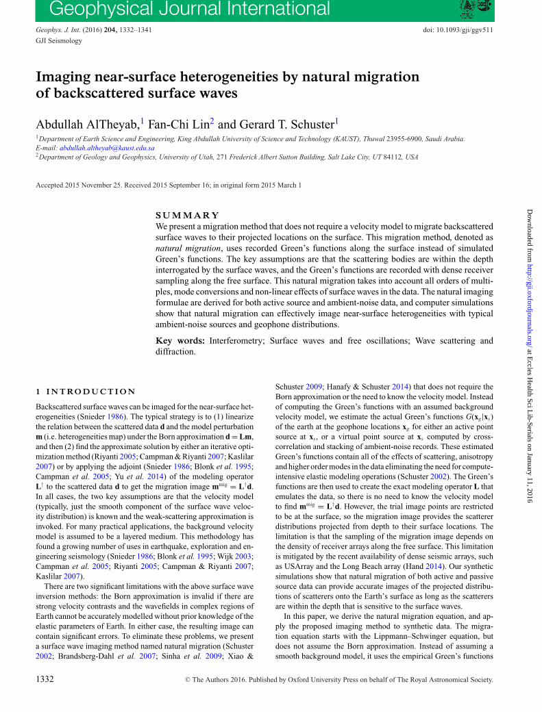
Figure 3. Muting of cross-correlated traces (A) to separate the direct (B)and scattered (C) events for natural migration. The first period (0.1 s) ismuted in the traces prior to migration.
record is simulated independently with five z-component noisesources emitting noise simultaneously; each source has a differ-ent signature as described above. The number of noise sources andthe length of each record are empirically determined to enhancethe quality of the empirical Green’s functions computed by cross-correlating the noise records. A similar quality can be achieved in
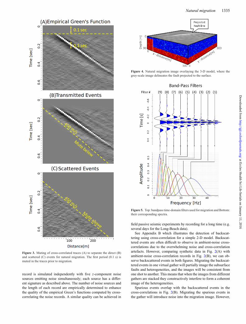
Figure 4. Natural migration image overlaying the 3-D model, where thegrey-scale image delineates the fault projected to the surface.
Figure 5. Top: bandpass time-domain filters used for migration and Bottom:their corresponding spectra.
field passive seismic experiments by recording for a long time (e.g.several days for the Long-Beach data).
See Appendix B which illustrates the detection of backscat-tering using cross-correlation for a simple 2-D model. Backscat-tered events are often difficult to observe in ambient-noise cross-correlations due to the overwhelming noise and cross-correlationartefacts. However, comparing synthetic data in Fig. 2(A) withambient-noise cross-correlation records in Fig. 2(B), we can ob-serve backscattered events in both figures. Migrating the backscat-tered events in one virtual gather will partially image the subsurfacefaults and heterogeneities, and the images will be consistent fromone shot to another. This means that when the images from differentgathers are stacked they constructively interfere to form a coherentimage of the heterogeneities.
Spurious events overlap with the backscattered events in thecross-correlations in Fig. 2(B). Migrating the spurious events inthe gather will introduce noise into the migration image. However,
Figure 6. Snapshots of laterally traveling Rayleigh waves using the bandpass filters as the source signatures. Note, the change of depth of penetration as afunction of frequency contents of bandpass range of frequencies.
such noise is unlikely to be consistent from virtual shot to another.Therefore, when the images are stacked noise will destructively in-terfere and be attenuated. We assume that this is also the case fordeep virtual reflections in the cross-correlations.
3.2 Natural migration procedure
Here, we describe the steps used to compute the natural migra-tion image from ambient-noise records, using the passive-data nat-ural migration equation (i.e. eq. 7). First, the recorded noise isspectrally normalized (Duret & Forgues 2015) (i.e. amplitudes inthe frequency domain are set to one) and then cross-correlated togenerate the empirical Green’s functions. The normalization andcross-correlation produce spectrally balanced Green’s functionswith zero-phase wavelet, so that it is suitable to assume γ l(ω) ≈ 1in the migration eq. (7). Next, we normalize the Green’s functionsin a virtual source gather by the maximum absolute value of the am-plitudes in the gather. We observe that this normalization partiallycorrects for the amplification effect that depends on the velocitynear the virtual source.
The second step is muting and wavefield separation. The samplesnear the zero lag are muted to avoid near-field strong artefact.1 Weempirically find that muting one period (estimated roughly from thetransmitted waves as shown in Fig. 3A) is sufficient to avoid strongartefacts near sources and receivers.
To compute the natural migration image, we need to separatetransmitted (i.e. direct) and scattered wavefields in the empiricalGreen’s functions so that
Cki (xA|xB) = C trans.ki (xA|xB) + C scat.
ki (xA|xB), (9)
where C trans.ki (xA|xB) contains the transmission events and
C scat.ki (xA|xB) contains only the scattered events. This separation
can be performed by muting, where an average velocity vavg. and
1This is related to singularities in the integration domain.
the period T of the direct arrivals are estimated and then used todesign the muting function,
τmute (x, xs) = |xs − x|vavg
+ T (10)
where the transmitted events are above the muting function and thescattered waves are below the function as shown in Figs 3(B) and(C), respectively. Smooth tapering is recommended when applyingthe mute.
The variables in the migration eq. (7) are defined using the sepa-rated wavefields as follows:
ui (xs |xr ) =∑
k
C scat.ki (xs |xr ), (11)
C0ki (x|xr ) = C trans.
ki (x|xr ), (12)
Clp(x|xs) = C trans.lp (x|xs) + C scat.
lp (x|xs). (13)
Note the summation in eq. (11) over the k index. In our numericalexample, however, we do not record horizontal components andtherefore we evaluate u1(xs |xr ) = C scat.
11 (xs |xr ) only.Now, we compute the natural migration image using eq. (7) and
substitute the separated transmission and scattered events respec-tively into the empirical Green’s functions and backscattered data(i.e. ui). Fig. 4 shows the natural migration result for the simpleexample above, where the migration image delineates the buriedfault. The fault image is a positive and negative doublet where thepositive values (white colour) identifies the slow part of the modeland the negative (black colour) identifies the fast side of the fault.The rest of the image has near zero values (grey) or filled withminor noise. Such noise is related to imperfect reconstruction ofthe Green’s function, and it can be reduced with longer passive datarecording, and a more uniform distribution of noise sources.
Surface waves travel laterally along the free surface, where thehorizontal boundaries between the layers do not cause backscatter-ing. Therefore, the proposed method cannot directly image changesin the medium along the depth axis, like boundaries between layers.This is useful when the objective of the seismic experiment is to
Figure 7. Natural migration images for different filters, where the decreas-ing dominant frequency of the filter acts as pesudo-depth. Lower frequencyfilters are displayed deeper and the higher frequencies are on top of the 3-Dnatural migration volume. The red arrows indicate the fault image.
image heterogeneities like faults and scatterers with disregard to thelayering details in the subsurface.
Natural migration images are evaluated at geophone stations onthe free surface at z = 0. Therefore, they do not directly indicatethe depth of the anomalies. To develop a sense of depth, we designmany bandpass filters βω′ with increasing peak frequency ω′, wherethe different frequency bands can be associated with different depthranges. The filters are chosen to cover the spectrum of the data,using any filter of choice. Frequencies are avoided that violate theNyquist sampling interval associated with geophone spacing.
Fig. 5 illustrates a set of bandpass filters in the time and frequencydomains. By solving the elastic wave equation using the averagevelocity of the first layer, we can estimate the sensitivity of theRayleigh waves to different depths of velocity anomalies, as shownin Fig. 6. For filters 1–3, most of the energy is concentrated at depthsshallower than that of the fault (15 m) and is unable to detect thefault. Filters with a lower range of frequencies, on the other hand,show the significant sensitivity of low-frequency Rayleigh waves todeeply buried velocity heterogeneities.
We also compute a collection of migration images for differentfrequency ranges that collectively gives an indication of relativedepths and sizes of the detected anomalies. Fig. 7 shows the naturalmigration images as a function of the filter’s range of frequen-cies. High-frequency filters 1–3 do not detect the fault, due to theRayleigh wave’s shallow depth of penetration. The remaining low-
Figure 8. A migration cross-section demonstrating the detection of thefault as a function of pseoudo-depth (filter number), where images of higherfrequency filters are displayed at the top and the lower ones are at the bottomof the cross-section. The arrow indicate the top of the fault at ω′ = 15 Hz,and the dashed line indicates the trace of the fault.
frequencies filter detects the fault. Fig. 8 shows a cross-sectionmigration image for y = 150 m, where the fault is seen clearly usingfilters from 4 to 9.
The same numerical experiment was repeated twice for the same3-D model but with fault depths of 21 and 30 m, and the corre-sponding natural migration images are shown in Figs 9 and 10,respectively. With increasing depth, the image of the fault becomesconfined to lower frequencies. In the natural migration images, dif-ferent frequencies detect the fault with different spatial resolution,where the filters with lower frequency ranges show the fault withlower resolution. This demonstrates the trade-off between depth ofpenetration and lateral resolution, which depends on the relationshipbetween frequency and depth of penetration of Rayleigh waves.
In general, the effectiveness of natural migration is limited bythe strength of the backscattered surface waves. This subject is cov-ered by Chai et al. (2012, 2014). We recommend using a syntheticdata test, as the one demonstrated above, for each case where nat-ural migration is applied to assess the abilities and the limits ofthe method in the given geological settings, noise distribution andsurvey geometry. In addition, applications of the method shouldbe in conjunction with other independent methods for studying thesubsurface, like surface wave tomography (Lin et al. 2008). This isto validate the interpretation of the natural migration images, and toreject possible false positives generated by uncorrelated noise andimperfect reconstruction of empirical Green’s functions.
4 C O N C LU S I O N S
The migration equations are derived for imaging backscat-tered waves using virtual Green’s functions computed by cross-correlating ambient noise. The benefits of this approach are that themigration velocity model is not needed for estimating the migra-tion Green’s functions and the actual physics of wave propagationare used for inversion. In addition, the Born approximation is notrequired and the computation of the adjoint operator requires min-imal computational resources. The key limitations are that a densereceiver coverage is required to construct a finely sampled image,and the current implementation is restricted to migration images onthe recording plane.
Figure 9. Natural migration images for a fault model where the fault is21 m deep.
Application of natural migration to the Long Beach array andUSArray (AlTheyab et al. 2014) will be the focus of future pub-lications. The backscattering migration provides complimentaryhigh-wavenumber information to the low-wavenumber transmis-sion tomographic image as is done in exploration seismology. Onepossibility in the future, is to invert for the perturbation in the least-squares sense, instead of using the migration equation (the adjoint).This however is non-trivial to compute for interferometric virtualgathers. In this paper, we migrated the backscattered events intopseudo-depths that depends on the frequency ranges of the data.Conversion to absolute depth requires some prior knowledge of thesubsurface velocities, and such conversion is the subject of an ongo-ing research. Another direction of interest is to analyse the couplingbetween incident Rayleigh-wave and Love scattered waves and viceversa.
A C K N OW L E D G E M E N T S
This publication is based upon work supported by the KAUSTOffice of Competitive Research Funds (OCRF) under award no.OCRF-2014-CRG3-62140387/ORS#2300. We thank the sponsorsfor supporting the Consortium of Subsurface Imaging and FluidModeling (CSIM). AlTheyab is grateful to Saudi ARAMCO forsponsoring his graduate studies. For computer time, this researchused the resources of the Supercomputing Laboratory at King Ab-dullah University of Science & Technology (KAUST) in Thuwal,Saudi Arabia.
Figure 10. Natural migration images for a fault model where the fault is30 m deep.
R E F E R E N C E S
AlTheyab, A., Workman, E.J., Lin, F.-C. & Schuster, G.T., 2014. Natu-ral migration of scattered surface waves from correlated ambient noise:applications on Long Beach array and US-array, in AGU Fall Meeting,Abstract S41A-4425.
Blonk, B. & Herman, G., 1994. Inverse scattering of surface waves: a newlook at surface consistency, Geophysics, 59(6), 963–972.
Blonk, B., Herman, G. & Drijkoningen, G., 1995. An elastodynamic inversescattering method for removing scattered surface waves from field data,Geophysics, 60(6), 1897–1905.
Brandsberg-Dahl, S., Hornby, B. & Xiao, X., 2007. Migration of surfaceseismic data with VSP Green’s functions, Leading Edge, 26(6), 778–780.
Campman, X. & Riyanti, C.D., 2007. Non-linear inversion of scatteredseismic surface waves, Geophys. J. Int., 171(3), 1118–1125.
Campman, X., van Wijk, K., Scales, J. & Herman, G., 2005. Imaging andsuppressing near-receiver scattered surface waves, Geophysics, 70(2),V21–V29.
Chai, H.-Y., Phoon, K.-K., Goh, S.-H. & Wei, C.-F., 2012. Some theo-retical and numerical observations on scattering of Rayleigh waves inmedia containing shallow rectangular cavities, J. appl. Geophys., 83, 107–119.
Chai, H.-Y., Goh, S.-H., Phoon, K.-K., Wei, C.-F. & Zhang, D.-J., 2014.Effects of source and cavity depths on wave fields in layered media,J. appl. Geophys., 107, 163–170.
Duret, F. & Forgues, E., 2015. 4D surface wave tomography using ambi-ent seismic noise, in 77th EAGE Conference and Exhibition—WorkshopsExtended abstract, EAGE, doi:10.3997/2214-4609.201413573.
Gottschammer, E. & Olsen, K.B., 2001. Accuracy of the explicit pla-nar free-surface boundary condition implemented in a fourth-order
Hanafy, S.M. & Schuster, G.T., 2014. Fault detection by surface seismicscanning tunneling macroscope: field test, in SEG Technical Program Ex-panded Abstracts, pp. 4608–4612, Society of Exploration Geophysicists.
Hand, E., 2014. A boom in boomless seismology, Science, 345(6198), 720–721.
Hudson, J.A. & Heritage, J.R., 1981. The use of the Born approximation inseismic scattering problems, Geophys. J. R. astr. Soc., 66(1), 221–240.
Kaslilar, A., 2007. Inverse scattering of surface waves: imaging of near-surface heterogeneities, Geophys. J. Int., 171(1), 352–367.
Larose, E. et al., 2006. Correlation of random wavefields: an interdisci-plinary review, Geophysics, 71(4), SI11–SI21.
Lin, F.-C., Moschetti, M.P. & Ritzwoller, M.H., 2008. Surface wave tomog-raphy of the western United States from ambient seismic noise: Rayleighand Love wave phase velocity maps, Geophys. J. Int., 173(1), 281–298.
Liu, Q. & Tromp, J., 2006. Finite-frequency kernels based on adjoint meth-ods, Bull. seism. Soc. Am., 96(6), 2383–2397.
Riyanti, C., 2005. Modeling and inversion of scattered surface waves, PhDthesis, Delft University of Technology.
Schuster, G.T., 2002. Reverse-time migration = generalized diffraction stackmigration, in SEG Technical Program Expanded Abstracts, pp. 1280–1283, Society of Exploration Geophysicists.
Schuster, G.T., 2010. Seismic Interferometry, Cambridge University Press.Schuster, G.T., Yu, J., Sheng, J. & Rickett, J., 2004. Interferometric/daylight
seismic imaging, Geophys. J. Int., 157(2), 838–852.Sinha, S., Hornby, B. & Ramkhelawan, R., 2009. 3D depth imaging of sur-
face seismic using VSP measured Green’s function, in SEG TechnicalProgram Expanded Abstracts 2009, pp. 4125–4128, Society of Explo-ration Geophysicists.
Snieder, R., 1986. 3-D linearized scattering of surface waves and a formalismfor surface wave holography, Geophys. J. Int., 84, 581–605.
Snieder, R., 2004. Extracting the Green’s function from the correlation ofcoda waves: a derivation based on stationary phase, Phys. Rev. E, 69,doi:10.1103/PhysRevE.69.046610.
Snieder, R. & Nolet, G., 1987. Linearized scattering of surface waves on aspherical Earth, J. Geophys., 61, 55–63..
Weaver, R.L. & Lobkis, O.I., 2004. Diffuse fields in open systems andthe emergence of the Green’s function (L), J. acoust. Soc. Am., 116(5),2731–2734.
Wijk, K., 2003. Multiple scattering of surface waves, PhD thesis, Center forWave Phenomena, Colorado School of Mines, Golden, Colorado.
Xiao, X. & Schuster, G., 2009. Local migration with extrapolated VSPGreen’s functions, Geophysics, 74(1), SI15–SI26.
Yu, H., Hanafy, S., Guo, B., Schuster, G.T. & Lin, F.-C., 2014. Directdetection of near-surface faults by migration of back-scattered surfacewaves, in SEG Technical Program Expanded Abstracts, pp. 2135–2139,Society of Exploration Geophysicists.
A P P E N D I X A : E F F E C T O F E L A S T I CH E T E RO G E N E I T I E S O N T H E NAT U R A LM I G R AT I O N I M A G E
From eq. (1), the scattered wavefield due to density perturbationscan be quantified using the following equation
ui (xs, xr ) =∫
ω2δpkγl (ω) Glp (x|xs) G0ki (x|xr )
× �ρ (x) d3x. (A1)
The corresponding migration equation (Liu & Tromp 2006) is
�ρ (x) =∫ ∫
xr �=x
∫xs �=x
ω2δpkγl (ω) Glp (x|xs) G0ki (x|xr )
× ui (xs, xr ) dxsdxr dω, (A2)
where the horizontal bar above the integration kernel indicates thecomplex conjugate of the kernel and the spatial integration is overthe source and receiver planes that exclude the imaging point. Thisavoids integrating over singular points in the Green’s tensors. Forconciseness, we omit the definition of the integration domain oversources and receivers throughout the manuscript.
Similarly, the scattered wavefield due to elastic tensor perturba-tions is
ui (xs, xr ) = −∫
γl (ω) (x)∂
∂xqGlp (x|xs)
× ∂
∂x jG0
ki (x|xr ) �ckjpq d3x, (A3)
so that the adjoint integral is
�ckjpq (x) = −∫∫∫
γl (ω)∂
∂xqGlp (x|xs)
∂
∂x jG0
ki (x|xr )
× ui (xs, xr ) dxr dxsdω, (A4)
where �ckjpq is the image corresponding to the perturbation of thetensor element indicated by the subscripts. Considering the sum ofmigration images for j = q, the migration equation above can beapproximated in the far field by
∑j
�ckjpj (x) ≈∫∫∫
ω2
v2 (x)γl (ω) Glp (x|xs) G0
ki (x|xr )
× ui (xs, xr ) dxr dxsdω, (A5)
where v (x) is the phase velocity for that mode of propagation (e.g.the phase velocity for monochromatic Rayleigh waves when mi-grating z-component backscattering using z-component incidentwavefield). Here, the spatial derivatives are approximated, un-der the far-field approximation, for a single mode of propagationusing∑
j
∂
∂x jGlp (x|xs)
∂
∂x jG0
ki (x|xr )
≈ − ω2
v2 (x)Glp (x|xs) G0
ki (x|xr ) . (A6)
Therefore,
v2 (x)∑
j
�ckjpj (x) =∫∫∫
ω2γl (ω) Glp (x|xs) G0ki (x|xr )
× ui (xs, xr ) dxr dxsdω. (A7)
The right-hand side above is the same as the migration equation fordensity (eq. A2) when p = k. This indicates that when we migratethe backscattered data using eq. (4), we can image both density andvelocity perturbations.
The sum of the images for density perturbations and the elastic-tensor perturbations (where j = q) gives the natural migrationimage
m (x) = �ρ (x) + v2 (x)∑j,p,k
�cpjk j (x)
=∫∫∫
ω2(1 + δpk
)γl (ω) Glp (x|xs) G0
ki (x|xr )
× ui (xs, xr ) dxr dxsdω, (A8)
In other words, the natural migration image is the sum of severalimages, each image is a geometric representation of the density
or elastic modulus perturbations. As a result, values in the imagesmight not be immediately useful, due to the entangled contributionsfrom different physical variables and the fact that the adjoint integralis not the inverse of the forward scattering equation. Nevertheless,the geometric information in the image is representative of theheterogeneities in the subsurface.
In our derivation above, we deliberately ignored contributions tothe images from the elastic-tensor perturbations for j �= p to avoidspatial derivatives, which numerically requires a dense samplingof naturally recorded Green’s functions. This does not necessarilymean that the perturbations in those elastic-tensor components can-not be imaged using eq. (4). Further research is needed to understandthe effects on those components in the migration image.
A P P E N D I X B : B A C K S C AT T E R E DE V E N T S I N A M B I E N T - N O I S EC RO S S - C O R R E L AT I O N S
In this section, we illustrate how backscattered events are detectedin the empirical Green’s function.
Empirical Green’s functions for the zz-components (i.e. C11) arecomputed by cross-correlating the recorded ambient-noise tracesaccording to eq. (5) as follows. For a given virtual source locatedon one of the stations, the recorded trace is referred to as the mas-ter trace. For each recording, the master trace is cross-correlatedwith the trace corresponding to a virtual receiver. Then, the cross-correlations for the given virtual source and receiver are stacked toform the empirical Green’s function for the virtual source–receiverpairs.
Fig. B1 depicts an empirical Green’s function for the simple 2-Dcase where a homogeneous model has a single scatterer. The promi-nent features in the gather are the transmitted waves highlighted bythe red dotted lines intersecting at the location of the virtual sourceat the zero-lag time. The rest of the empirical function is domi-
Figure B1. A shot gather of an empirical Green’s function computed bycross-correlating ambient noise. The red triangle denotes the lateral positionof the virtual source (i.e. the master-trace position for the cross-correlation)and the green dashed line denotes the position of a scatterer.
nated by spurious events which are the result of cross-correlatingirrelevant events. Such spurious events are weakened with longerrecording time. Nevertheless, some key backscattering events canbe identified and are highlighted in the yellow dashed lines andlabelled A, B, C in Fig. B1.
The backscattered events are the result of cross-correlatingbackscattered waves with transmitted events in the ambient noise.The cross-correlation and stacking process of events in the ambient-noise records eliminates common ray paths (Schuster et al. 2004;Schuster 2010), that is∑
n
eiωτnr e−iωτns ≈ eiωτsr , (B1)
for ambient-noise sources located at n, where τ ns denotes the trav-eltime from the noise source n to the virtual source s, and similarlyτ nr is the traveltime from the noise source to the virtual receiver r.In this simplified analysis of kinematics, we harmlessly ignore theamplitudes and dispersion and highlight the phase of the correlated
Figure B2. Ambient-noise cross-correlation scenarios that give rise to thebackscattering events in Fig. B1. The start symbol � denotes convolutionbetween the conjugated phases, shown as dashed lines from the noise sourceto the virtual source and phases from noise source to the virtual receivershown as a solid line.
arrival. Using this simple notion of canceling the phase of com-mon ray paths by cross-correlation, we can analyse the backscatter-ing events in the empirical Green’s functions. Fig. B2 depicts thethree scenarios for redatuming passive events into the A-, B- andC-labelled backscattered events in the empirical Green’s functionin Fig. B1.
The A-labelled event in Fig. B1 is characterized by acausal scat-tering excited by an acausal incident wave. As demonstrated by thecorresponding plot labelled A in Fig. B2, this event is the result ofcross-correlating backscattered events from a scatterer at the virtualsource position with the direct arrival at the virtual receiver posi-tion. The common ray path is eliminated and the results indicatean event that travels from the virtual source to the scatterer to thevirtual receiver, that is∑
n
eiωτnr e−iωτnXs ≈ e−iωτs Xr , (B2)
where X is the position of the scatterer and the τ subscripts denotethe points along the ray path. However, this event has a negativephase (dashed lines Fig. B2 indicate negative phase), and thereforeit appears at a negative time lag in the empirical Green’s functionin Fig. B1. Similarly, the C-labelled event is the result of cross-correlating the direct arrival associated with the virtual source po-sition and the backscattered events at the virtual receiver position.Therefore, the phase delay associated with the common ray path is
eliminated, giving rise to a causal scattering event due to a causalincident wave that appears in the positive time lag in the empiricalGreen’s function (eiωτs Xr ).
The remaining B-labelled event is related to cases where thescatterer is between the virtual source and receiver positions. Insuch cases, backscattered events are cross-correlated with directevents, or vice versa, giving rise to a mixed phase (eiωτXr −iωτs X ),where the event could appear at either positive or negative timelags of the empirical Green’s function. In all cases, however,the negative phase associated with events traveling from the vir-tual source to the scatterer while the positive phase is associ-ated with events traveling from the scatterer to the virtual re-ceiver shown in Fig. B2(B). Therefore, the B-labelled backscat-tered event is causal backscattering due to acausal incident waves.If cross-correlation is time symmetric as defined in eq. (5), amirror of the B-labelled event will be in the empirical Green’sfunction, which is acausal backscattering due to causal incidentwaves.
The B-labelled backscattering event can be considered non-physical and contradictory to eq. (6). Such non-physical scatter-ing, however, is redundant information and often overlaps withearly arrivals like body waves and strong cross-correlation arte-facts. Therefore, we mute such events between the causal- andacausal-transmitted events in the ambient-noise cross-correlationbefore migration.