Imaging Study for Small Unmanned Aerial Vehicle (UAV ... · SUPPLEMENTARY NOTES. 14. ABSTRACT ......

ARL-TR-8654 MAR 2019

Imaging Study for Small Unmanned Aerial Vehicle (UAV)-Mounted Ground-Penetrating Radar: Part I – Methodology and Analytic Formulation by Traian Dogaru Approved for public release; distribution is unlimited.

NOTICES

Disclaimers

The findings in this report are not to be construed as an official Department of the Army position unless so designated by other authorized documents. Citation of manufacturer’s or trade names does not constitute an official endorsement or approval of the use thereof. DESTRUCTION NOTICE—For classified documents, follow the procedures in DOD 5220.22-M, National Industrial Security Program Operating Manual, Chapter 5, Section 7, or DOD 5200.1-R, Information Security Program Regulation, C6.7. For unclassified, limited documents, destroy by any method that will prevent disclosure of contents or reconstruction of the document.

ARL-TR-8654 MAR 2019

Imaging Study for Small Unmanned Aerial Vehicle (UAV)-Mounted Ground-Penetrating Radar: Part I – Methodology and Analytic Formulation by Traian Dogaru Sensors and Electron Devices Directorate, CCDC Army Research Laboratory Approved for public release; distribution is unlimited.

ii

REPORT DOCUMENTATION PAGE Form Approved OMB No. 0704-0188

Public reporting burden for this collection of information is estimated to average 1 hour per response, including the time for reviewing instructions, searching existing data sources, gathering and maintaining the data needed, and completing and reviewing the collection information. Send comments regarding this burden estimate or any other aspect of this collection of information, including suggestions for reducing the burden, to Department of Defense, Washington Headquarters Services, Directorate for Information Operations and Reports (0704-0188), 1215 Jefferson Davis Highway, Suite 1204, Arlington, VA 22202-4302. Respondents should be aware that notwithstanding any other provision of law, no person shall be subject to any penalty for failing to comply with a collection of information if it does not display a currently valid OMB control number. PLEASE DO NOT RETURN YOUR FORM TO THE ABOVE ADDRESS.

1. REPORT DATE (DD-MM-YYYY)

March 2019 2. REPORT TYPE

Technical Report 3. DATES COVERED (From - To)

September 2018–January 2019 4. TITLE AND SUBTITLE

Imaging Study for Small Unmanned Aerial Vehicle (UAV)-Mounted Ground-Penetrating Radar: Part I – Methodology and Analytic Formulation

5a. CONTRACT NUMBER

5b. GRANT NUMBER

5c. PROGRAM ELEMENT NUMBER

6. AUTHOR(S)

Traian Dogaru 5d. PROJECT NUMBER

5e. TASK NUMBER

5f. WORK UNIT NUMBER

7. PERFORMING ORGANIZATION NAME(S) AND ADDRESS(ES)

Combat Capabilities Development Command, Army Research Laboratory ATTN: FCDD-RLS-RU 2800 Power Mill Road Adelphi, MD 20783-1138

8. PERFORMING ORGANIZATION REPORT NUMBER

ARL-TR-8654

9. SPONSORING/MONITORING AGENCY NAME(S) AND ADDRESS(ES)

10. SPONSOR/MONITOR'S ACRONYM(S)

11. SPONSOR/MONITOR'S REPORT NUMBER(S)

12. DISTRIBUTION/AVAILABILITY STATEMENT

Approved for public release; distribution is unlimited.

13. SUPPLEMENTARY NOTES

14. ABSTRACT

This report is the first part of an investigation of possible configurations for a ground-penetrating radar (GPR) system installed on a small unmanned aerial vehicle platform and used for buried target imaging. After discussing the advantages of this type of platform compared with existing designs, we develop the tools needed to analyze the imaging performance of the proposed system. This is done primarily by simulating the point spread function (PSF) of the system working in either down-looking or side-looking configuration and horizontal-horizontal or vertical-vertical polarization. The current work lays the theoretical foundations and describes the methodology employed in the GPR imaging system’s performance analysis, discussing the calculation of the point target response, the formulation of the imaging algorithm, and the equations employed in the PSF numeric models.

15. SUBJECT TERMS

ground penetrating radar, synthetic aperture radar, radar imaging, point spread function, radar modeling

16. SECURITY CLASSIFICATION OF: 17. LIMITATION OF ABSTRACT

UU

18. NUMBER OF PAGES

45

19a. NAME OF RESPONSIBLE PERSON

Traian Dogaru a. REPORT

Unclassified b. ABSTRACT

Unclassified

c. THIS PAGE

Unclassified

19b. TELEPHONE NUMBER (Include area code)

(301) 394-1482 Standard Form 298 (Rev. 8/98)

Prescribed by ANSI Std. Z39.18

Approved for public release; distribution unlimited. iii

Contents

List of Figures iv

1. Introduction 1

2. Desirable GPR System Performance, Current State of the Art, and Proposed UAV-based Configurations 2

3. Modeling Approaches and Analytic Formulation 8

3.1 SAR Imaging System Modeling Approaches and Scenarios 8

3.2 Analytic Calculation of the PTR 12

3.3 Validation of the PTR Analytic Formulation 20

3.4 SAR Imaging Algorithm Formulation 24

3.5 Accounting for the Ground Bounce 27

4. Conclusions 29

5. References 30

Appendix. Calculation of the Propagation Path for Ground-Penetrating Radar (GPR) 33

List of Symbols, Abbreviations, and Acronyms 38

Distribution List 39

Approved for public release; distribution unlimited. iv

List of Figures

Fig. 1 B-scan radar mapping technique in down-looking GPR: a) schematic representation of the scanning principle and b) actual B-scan of a buried landmine obtained by AFDTD computer simulation ................ 4

Fig. 2 Schematic representation of a GPR system with the dipole antenna placed close to the ground, showing the self-focusing effect of the beam upon propagation into the ground ............................................... 5

Fig. 3 Dipole antenna patterns in a GPR SAR system for horizontal and vertical dipole orientations .................................................................... 8

Fig. 4 GPR SAR system using a linear synthetic aperture in down-looking configuration: a) perspective view, b) top view, and c) side view ..... 10

Fig. 5 GPR SAR system using a linear synthetic aperture in side-looking configuration: a) perspective view and b) top view ............................ 10

Fig. 6 Geometry involved in the propagation path (green line) between radar and target consistent with the Green’s function asymptotic expansion: a) top view and b) side view in the u-v plane. Note that v is the vertical axis going through the point target. ....................................... 19

Fig. 7 Comparison of the PTR as a function of position along the synthetic aperture, computed by the analytic formulas and AFDTD simulations for down-looking configuration: a) magnitude in decibels and b) phase in degrees ............................................................................................ 21

Fig. 8 Comparison of the PTR as a function of position along the synthetic aperture, computed by the analytic formulas and AFDTD simulations for side-looking configuration: a) magnitude in decibels and b) phase in degrees ............................................................................................ 22

Fig. 9 Comparison of various components of the PTR as a function of position along the synthetic aperture, computed by AFDTD simulation: a) down-looking configuration and b) side-looking configuration ....................................................................................... 23

Fig. 10 Comparison of the PTR as a function of position along the synthetic aperture, computed by the analytic formulas and AFDTD simulations of scattering by a metallic sphere: a) down-looking configuration and b) side-looking configuration .............................................................. 23

Fig. A-1 Geometry involved in the propagation path (green line) between radar and target consistent with Snell’s law: a) top view and b) side view in the u-v plane. Note that v is the vertical axis going through the point target. .................................................................................................. 34

Approved for public release; distribution unlimited. 1

1. Introduction

Detection of objects buried underground is a major application of radar technology dating back several decades. Ground-penetrating radar (GPR) has been employed for purposes as diverse as mapping soil layers, bedrocks, and water tables; finding buried utility lines; exploring archeological and forensic investigation sites; and assessing the structural integrity of roads, bridges, and runways.1–3 An important military application of GPR is detecting buried explosive hazards, including landmines, unexploded ordnance, and a wide variety of improvised explosive devices.

The Combat Capabilities Development Command, Army Research Laboratory (ARL), has been at the forefront of this technology for more than 20 years, conducting various Department of Defense (DOD) counter-explosive hazard (CEH) programs. Our developments in GPR systems have been closely linked to ultra-wideband (UWB) and synthetic aperture radar (SAR) technologies. Several generations of radar systems have been designed and built at ARL for this purpose: the BoomSAR,4 the Synchronous Impulse Reconstruction (SIRE),5 and the Spectrally Agile Frequency-Incrementing Reconfigurable (SAFIRE)6 radars. Other ARL efforts included a large number of studies related to GPR phenomenology and signal processing, as well as analyses of other commercial and DOD-sponsored GPR systems.

Among the various GPR design solutions currently available for CEH applications, we distinguish three major sensing geometries: down-looking, side-looking, and forward-looking. Examples of down-looking GPR include the vehicle-mounted Chemring Sensors and Electronic Systems (formerly known as NIITEK),7 as well as the handheld L-3 Security and Detection Systems radar.8 A typical side-looking SAR system for GPR applications is the Mirage radar9 mounted on an airborne platform. Examples of forward-looking radars for the same applications are the already mentioned SIRE and SAFIRE systems, as well as the iRadar, developed at the Lawrence Livermore National Laboratory.10 A more comprehensive list of GPR systems developed specifically for landmine detection can be found in Witten11 and Daniels12 (note that some of this information is currently dated). While each of these technological solutions has certain merits, all of them suffer from major limitations, which keeps the CEH efforts an active area of investigations.

The recent advent of small unmanned aerial vehicle (sUAV) technology has created new opportunities for radar system operational concepts, including GPR-related applications. Thus, sUAV-mounted sensors can perform the rapid surveillance of large areas with minimal human supervision while avoiding contact with the


ground. Additionally, these devices can fly close to the ground, which involves smaller ranges than conventional high-altitude airborne radar platforms. In effect, the flexibility and affordability of sUAV platforms represents a game changer in GPR technology. New research studies are required to explore and fully exploit all the possibilities opened by this sensing modality. A recently published paper13 describing a GPR mounted on a commercially available DJI Technology platform demonstrates this technology’s capabilities, while investigations by other research groups are currently underway.

This two-part study takes an in-depth look at the GPR technology from a radar imaging perspective, in particular the buried target imaging performance afforded by such a system as a function of radar parameters that include frequency, polarization, and sensing geometry. The performance assessment is based on computer models. While no particular sUAV platform for the radar system is defined, the geometries considered in our models are compatible with a generic platform of this type.

Part I of this investigation, which is primarily concerned with describing the modeling methodology and analytic formulation, is organized as follows. Section 2 reviews the main attributes required from a GPR system and the current state of the art in this technology and describes the proposed sUAV-based GPR configurations. In Section 3 we develop the modeling methodology, with emphasis on the mathematical formulation of the point target response and the imaging algorithm. Section 4 draws the conclusions of Part I. Part II of the investigation, to be published in a subsequent report, will present simulation results obtained by 2-D and 3-D sensing geometries and various radar parameters, with an emphasis on system performance characterization.

2. Desirable GPR System Performance, Current State of the Art, and Proposed UAV-based Configurations

A GPR system typically works by propagating a wideband low-frequency electromagnetic (EM) wave inside the ground and receiving back the wave scattered by any kind of material inhomogeneities present along the propagation path. The radar antennas are physically moved along a track parallel to the ground surface, effectively scanning a given area for possible targets. The scanning can sometimes be combined with SAR imaging techniques. A list of desirable GPR system performance attributes and commonly used design solutions includes the following:


• Good penetration of radar waves inside the ground. This requires using relatively low frequencies in the microwave spectrum, typically below 3 GHz, depending on the anticipated target depth.

• Good resolution and target localization in all spatial dimensions. This is important in the target detection process, as well as in separating the target from clutter (distributed or discrete). To achieve that, GPR systems typically use UWB waveforms (with fractional bandwidths around 100% being common) and sometimes perform wide-angle SAR integration.

• Good clutter rejection. Two major clutter items that affect GPR performance are the air–ground interface (the so-called “ground bounce”, which is discrete or localized in nature) and rough-ground surface scattering (which is distributed over an area). Ground bounce is particularly relevant to down-looking sensing geometries and can be mitigated by using a side-looking geometry instead. On the other hand, distributed surface clutter has a significant impact on the side-looking geometries.

• Low sidelobes and grating lobes in the radar image. These are again important in the target detection and discrimination processes and are relevant to systems performing SAR imaging. The classic methods used in suppressing these artefacts are tapering of the synthetic antenna aperture (against sidelobes) and high-rate along-track sampling (against grating lobes).

• Low transmitted power. This is a desirable attribute in any radar system since it lowers the system cost, makes the radar difficult to detect/intercept, and may be required by existing EM spectrum regulations. The principal way to ensure satisfactory performance with low power is to operate the radar system at small ranges.

• Sufficient standoff detection range. This requirement is somewhat contradictory to the previous one but is essential in CEH applications, where often the target must be detected ahead of the vehicle driving over it. The most obvious solution to this issue is mounting the radar system on an airborne platform; however, this typically results in a significant increase in system cost and complexity.

• Rapid coverage of a large area. This can be more readily achieved from long-range airborne platforms than from close-to-ground down-looking GPR systems. Note that the latter require either 2-D scanning (single antenna systems) or an antenna array to completely localize the target in 3-D.


• Low size, weight, and power, and cost. Again, this is a desirable attribute for any radar system and may be critical in operating the sensor onboard an airborne platform. One component requiring special attention is the radar antenna, which ideally should have low profile and be easy to fabricate while providing good performance across a wide range of frequencies.

As already mentioned in the Introduction, three types of sensing geometries are currently used for GPR systems: down-looking, side-looking, and forward-looking. The vast majority of the literature dedicated to GPR technology focuses on the down-looking sensing geometry, which is also the most widespread in existing GPR systems. Among the advantages of the down-looking GPR configuration is the low-to-ground operating range, which requires low transmitted power, provides good coupling of the radar wave into the ground, and typically ensures good resolution of the radar maps. Additionally, the vertical-plane orientation of these maps provides information on the target depth. One major drawback of these systems is the strong ground bounce, which may compete with the target response. Another limitation, particularly problematic to radar sensors mounted on ground vehicles, is the absence of any significant standoff range.

One interesting aspect of most existing down-looking GPR systems is that they create B-scan radar maps in vertical planes2 and rarely employ SAR imaging techniques in the process. A B-scan map consists of concatenating the range profiles in the depth direction, obtained while scanning the area of interest along a track parallel to the ground surface. A schematic representation of this scanning technique and a B-scan of a buried landmine obtained by ARL Finite-Difference Time-Domain (AFDTD) computer simulation are shown in Fig. 1.

Fig. 1 B-scan radar mapping technique in down-looking GPR: a) schematic representation of the scanning principle and b) actual B-scan of a buried landmine obtained by AFDTD computer simulation

To explain why SAR imaging techniques are avoided by many of these systems, it helps to remember that one major reason for performing SAR processing is to focus an equivalent narrow radar beam by combining several wide and divergent antenna

(a) (b)


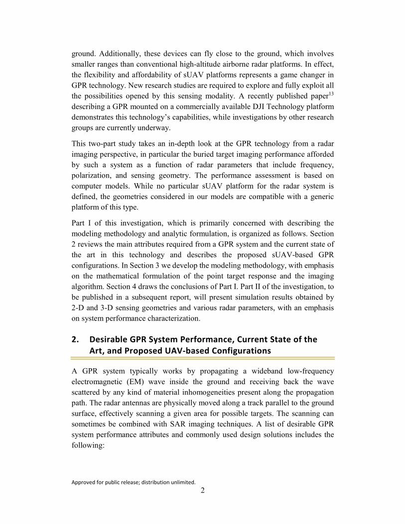
beams in the synthetic aperture. This type of processing is essential to obtaining good cross-range resolution in long-range radar, where the spatial beam divergence is proportional to the range. However, in close-to-ground down-looking GPR, the ranges are very small, sometimes on the order of a wavelength (0.2–0.3 m). An analysis of the wave propagation in this type of environment14 reveals a self-focusing effect of the antenna beam at the transition between the air and ground media (Fig. 2). As a result, the overwhelming contribution to the radar response comes from scatterers positioned directly below the antenna location. Consequently, simple B-scans obtained by close-to-ground down-looking GPR systems provide sufficient lateral (or cross-range) resolution to enable adequate detection performance for most targets of interest.

Fig. 2 Schematic representation of a GPR system with the dipole antenna placed close to the ground, showing the self-focusing effect of the beam upon propagation into the ground

Another important discussion related to down-looking GPR systems is the issue of the ground bounce effect on target detection, or, more generally, on the radar map quality. It is clear from the B-scan shown in Fig. 1b that the reflection from the air–ground interface produces a radar response orders of magnitude stronger than the target scattering. In the case of shallow-buried targets with weak reflectivity, it may be difficult to separate them from the ground-bounce sidelobes in the radar map. Therefore, clutter suppression schemes for ground-bounce mitigation have been developed by the GPR community. A typical suppression procedure consists of subtracting the average signal from previous along-track samples from the current range profile. Nevertheless, these ground-bounce mitigation techniques have their limitations and typically yield a clutter reduction of about 20 dB.15 Possible reasons for not achieving perfect ground-bounce cancellation include rough interface profile statistics that may change along the track; small changes in the distance from sensor to interface; the presence of scattering from other sources, such as soil inhomogeneities; and hardware-induced errors.


Side-looking GPR sensing geometries mitigate the specular ground-bounce issue by directing it to away from the radar receiver. These GPR systems are typically installed on airborne platforms and operate as more-or-less conventional strip-map SAR systems. SAR processing is required in creating radar terrain maps since the range is usually large (typically on the order of kilometers). These radar images are formed in the horizontal ground plane; therefore, the downrange direction has a different meaning than in down-looking GPR systems. Although the SAR images created in side-looking geometry can have good resolution (about 0.2–0.3 m) in down- and cross-range directions, they offer no information on the target depth. In general, these sensors are more effective for shallow-buried targets than for deep-buried ones and require much larger transmitted power than close-to-ground down-looking GPR systems.

The major source of clutter for the side-looking GPR sensing geometry is the irregular ground surface, which always creates some amount of backscattering response to the radar receiver. This type of clutter is distributed over the entire image area and is random (incoherent) in nature, so there are no effective ways to predict and suppress it when the targets are stationary. Both modeling16 and experimental17 studies have demonstrated the difficulty of detecting weak buried targets (such as plastic landmines) by side-looking GPR systems, even in mild clutter conditions.

The forward-looking GPR sensing geometry5 achieves some kind of compromise between the two previous modalities. Thus, the scanning trajectory is somewhat similar to that of down-looking systems, but the antennas are tilted to look ahead of the platform instead of straight down. As a result, the ground bounce is directed away from the receiver, and the system achieves a certain amount of standoff range. However, the images are created in the ground plane (same as in the side-looking case) and suffer from the same limitations produced by rough-ground clutter previously discussed. Additionally, the forward-looking GPR systems need to be equipped with an antenna array to achieve resolution in the across-track direction, and their design is usually more complex than for the other sensing modalities.

The sUAV-based GPR system we envision will be equipped with one transmitter–receiver (Tx–Rx) antenna pair, fly close to ground, and scan the terrain in a manner similar to strip-map SAR systems. Mounting the sensor on an airborne platform eliminates the standoff range issue characteristic to ground vehicle platforms. Additionally, unlike full-scale airborne platforms used in conventional side-looking GPR, the sUAV carrying the radar can fly at very low altitudes, reducing the system cost and required transmitted power. Although operating at small ranges, the sUAV-based GPR will employ SAR-type processing, which ideally should allow the target localization in the 3-D space.


One important question this study attempts to answer is which of the down-looking or side-looking sensing geometries yields better performance for buried target imaging and detection. Some of the pros and cons of these two configurations were already mentioned in Section 2 and will be further expanded by the numerical examples in Part II of this investigation.

Another radar system parameter is polarization. A survey of the literature on down-looking GPR reveals that all existing systems using this geometry operate with horizontal-horizontal (H-H) polarization, where the electric field generated by the antenna is predominantly oriented in a horizontal plane. (Note: The circular polarization used by some GPR designs11 is also a variant of H-H polarization, where the ratio between the fields along two horizontal Cartesian directions can be set to the desired complex value.) This seems a logical choice, given that H-H polarization offers the best coupling of the EM wave generated by a dipole-like antenna to an underground region located straight below this antenna. However, several recent papers18,19 have suggested that vertical-vertical (V-V) polarization coupled with SAR processing can also be used to image underground targets, especially when the antennas are slightly elevated from the ground level. In this report, we explore both polarization options for GPR systems and compare their performance based on computer models.

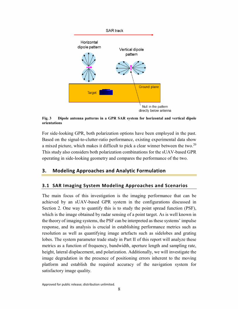
A qualitative illustration of the difference between the two polarization options is depicted in Fig. 3, which shows a schematic representation of a dipole antenna’s pattern when oriented horizontally or vertically. For the horizontal dipole, the maximum gain is achieved in a direction straight underneath the antenna. This justifies our statement that the H-H polarization offers the best wave coupling into the ground for down-looking GPR. At the same time, this configuration is characterized by a strong ground-bounce response. On the other hand, the vertical dipole’s pattern has a null in the straight-down direction, which suppresses the ground-bounce response to the Rx (to be exact, a residual field is still present in that direction but of much lower magnitude than in the horizontal dipole case). However, when the Tx–Rx antenna pair is moved along the SAR track, the target scattering response is still coupled with the vertical dipoles at positions characterized by an oblique angle between the two. Along-track integration of these responses by SAR processing then results in an image with a target-to-ground-bounce ratio larger than in the horizontal polarization.


Fig. 3 Dipole antenna patterns in a GPR SAR system for horizontal and vertical dipole orientations

For side-looking GPR, both polarization options have been employed in the past. Based on the signal-to-clutter-ratio performance, existing experimental data show a mixed picture, which makes it difficult to pick a clear winner between the two.20 This study also considers both polarization combinations for the sUAV-based GPR operating in side-looking geometry and compares the performance of the two.

3. Modeling Approaches and Analytic Formulation

3.1 SAR Imaging System Modeling Approaches and Scenarios

The main focus of this investigation is the imaging performance that can be achieved by an sUAV-based GPR system in the configurations discussed in Section 2. One way to quantify this is to study the point spread function (PSF), which is the image obtained by radar sensing of a point target. As is well known in the theory of imaging systems, the PSF can be interpreted as these systems’ impulse response, and its analysis is crucial in establishing performance metrics such as resolution as well as quantifying image artefacts such as sidelobes and grating lobes. The system parameter trade study in Part II of this report will analyze these metrics as a function of frequency, bandwidth, aperture length and sampling rate, height, lateral displacement, and polarization. Additionally, we will investigate the image degradation in the presence of positioning errors inherent to the moving platform and establish the required accuracy of the navigation system for satisfactory image quality.


A more realistic modeling scenario presented in Part II will employ the AFDTD software21 in simulating radar scattering by a landmine buried underground, with a rough surface included as an additional option. As described in multiple previous ARL publications, this software, based on the finite-difference time-domain (FDTD) algorithm, was developed entirely in-house for simulating a wide variety of radar sensing scenarios. One of the features unique to this code is the accurate treatment of scattering by targets placed in a half-space (or air–ground) configuration, which makes it particularly well-suited for the imaging study in this report. Another feature of the AFDTD software useful to our sensing scenario is the inclusion of a rough ground surface, allowing us to quantify its effect on the SAR image quality.

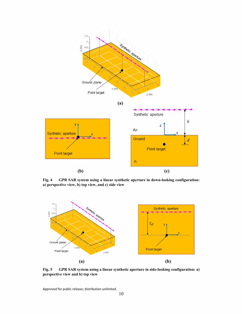
The geometry of a GPR system using 2-D SAR processing is illustrated in Fig. 4 (for down-looking GPR) and Fig. 5 (for side-looking GPR), which show all of the parameters relevant to the analysis performed here. The down-looking configuration assumes that the linear synthetic aperture passes directly above the buried target. Since we do not know the target location a priori, this particular geometry is only seldom encountered in practice. In fact, in the most-common scenarios, the radar operates in a side-looking configuration with various lateral aperture offsets with respect to the target position. Nevertheless, investigating the down-looking geometry for GPR systems is of major interest as a limit case in a continuum of aperture offsets for side-looking configurations.


Fig. 4 GPR SAR system using a linear synthetic aperture in down-looking configuration: a) perspective view, b) top view, and c) side view

Fig. 5 GPR SAR system using a linear synthetic aperture in side-looking configuration: a) perspective view and b) top view

(a)

(b) (c)

(a) (b)


The following key assumptions regarding the GPR system considered in this study make the SAR processing effective for detecting underground targets: 1) the radar platform flies at a height of at least several wavelengths, 2) the target is buried at shallow depth (no more than 0.3 m from the surface), and 3) the soil exhibits low loss. Coincidentally, these conditions are also required by some of the approximations used in the mathematical formulation developed in this section. Other authors14 have discussed the fundamental limitations of GPR SAR imaging techniques for deeply buried targets in highly lossy soils.

The antennas are always modeled as small dipoles, which is entirely adequate for this study. Other wide-beam antenna patterns can be accommodated by the modeling approach described here by introducing certain weights to the aperture samples involved in the SAR image formation algorithm. Note that throughout this report we only consider monostatic radar configurations. To be more precise, in the PSF analysis the Tx and Rx antennas are exactly collocated at each aperture sample position, whereas in the AFDTD simulations the two antennas are slightly displaced with respect to one another (we call that a quasi-monostatic geometry).

For the SAR imaging algorithm, we use the matched filter method,22 which is a general and accurate procedure that can be applied to arbitrary 3-D aperture geometries and bistatic radar configurations. The most general formulation (assuming a monostatic SAR geometry) can be written as

( ) ( ) ( )∑∑= =

=L

l

M

mmlml fHfP

LMI

1 1,,,1 rrrr , (1)

where ( )rI is the complex image voxel value at position vector [ ]Tzyx=r , ( )mlfP r, is the complex radar sample received at aperture index m and frequency

index l, L and M represent the number of samples in frequency and synthetic aperture position, respectively, and ( )rr ,, mlfH represents the matched filter’s transfer function, which depends on the frequency and the positions of the radar and image voxel, respectively. In the classic matched filter theory, ( )rr ,, mlfH is taken as the conjugate of the response of a point target placed in position r, with the radar in position rm:

( ) ( )rrrr ,,PTR,, mlml ffH ∗= . (2)

Given the importance of the point target response (PTR) for SAR image analysis, we dedicate a large portion of this section to its derivation for the configurations described by Figs. 4 and 5. Note that the presence of the air–ground interface (or the half-space configuration) makes this analysis much more complex than the


traditional treatment of radar wave propagation and scattering that assumes a free-space environment. Additionally, the usual far-field conditions valid for most other radar sensing scenarios cannot be invoked in our case, where the radar antennas are placed relatively close to the target. Rigorously speaking, the PTR for our half-space scenario cannot be described by an analytic formulation. Nevertheless, by making a series of approximations, we can develop some relatively simple equations giving us important insight into the radar wave propagation phenomenology and SAR system imaging performance.

3.2 Analytic Calculation of the PTR

The radar wave propagation and scattering phenomenology relevant to the PTR calculation can be described in words as follows. The Tx dipole at aperture sample m, characterized by the dipole moment ( )m

t rIl , generates an EM field incident upon the target positioned at r0, which in turn induces equivalent currents on the target surface or volume. Since in our case the target is a point, the induced currents take the dimension of a secondary dipole moment, which creates the scattered EM field. This field is propagated to the Rx antenna corresponding to the same aperture sample, where the received signal is proportional to the scattered electric field in that region ( )m

r rE . Formally, this process can be described by the following equation:

( ) ( )[ ] ( )[ ] ( )[ ] ( )mt

mmmr rIlrrGrρrrGrE 21

0012

0 ,, →→= . (3)

The symbols ( )[ ] 210 , →

mrrG and ( )[ ] 120, →rrG m stand for the Green’s function

dyadic23 characterizing the propagation between the transmitter and target and between the target and receiver, respectively, while ( )[ ]0rρ represents the target

reflectivity. To be more specific, the ( )[ ] 210 , →

mrrG notation means the Green’s function dyadic linking the dipole moment of a Tx placed in medium 1 (air) at position [ ]Tmmmm zyx=r to the electric field received in medium 2 (ground) at

position [ ]Tzyx 0000 =r . In our GPR system geometry, we have mz h= and

0z d= − . Note that the Green’s function dyadics are described by 3 × 3 matrices, while the reflectivity is described by a 3 × 3 tensor (the square brackets around these quantities are meant to distinguish them from vector quantities such as Il or E). In Cartesian coordinates, the previous equation can be written explicitly as the following:


=

→→→

→→→

→→→

→→→

→→→

→→→

tz

ty

tx

zzzyzx

yzyyyx

xzxyxx

zzzyzx

yzyyyx

xzxyxx

zzzyzx

yzyyyx

xzxyxx

tz

ry

rx

IlIlIl

GGGGGGGGG

GGGGGGGGG

EEE

212121

212121

212121

121212

121212

121212

ρρρρρρρρρ

. (4)

To explain the notations in this equation, we note that, for instance, 21→xyG is the

scalar Green’s function linking a y-oriented Tx dipole placed in medium 1 to the x component of the Rx field located in medium 2. Also note that in Eq. 4 we dropped the coordinates of the aperture sample and point target (rm and r0, respectively) to simplify the expressions.

The elements of the ( )[ ]0rρ tensor, which we loosely called “target reflectivity”, provide the links between various components of the electric field incident on the target and those of the currents (more specifically, the dipole moments) induced in the target. While these elements are not directly associated with a particular physical quantity, they play a role similar to the elements of the scattering matrix,24 which are more familiar to the radar engineer. Note, though, that the scattering matrix is a concept valid only for far-field radar configurations, and its elements have a dimensionality that differs from those of the reflectivity tensor introduced here (m vs. Ω–1m2, respectively).

We can also rewrite Eq. 4 using spherical coordinates r, φ, and θ in the target region, while keeping the Cartesian coordinate notation in the Tx–Rx region.

=

→→→

→→→

→→→

→→→

→→→

→→→

tz

ty

tx

zyx

zyx

rzryrx

r

r

rrrr

zzzr

yyyr

xxxr

rz

ry

rx

IlIlIl

GGGGGGGGG

GGGGGGGGG

EEE

212121

212121

212121

121212

121212

121212

θθθ

φφφ

θθθφθ

φθφφφ

θφ

θφ

θφ

θφ

ρρρρρρρρρ

. (5)

The advantage of the spherical coordinate notation is that the elements of ( )[ ]0rρ become more closely connected with the traditional polarization combinations used in target scattering analysis, such as V-V, H-H, and so on. However, since the concepts of vertical or horizontal polarization cannot be rigorously defined in our near-field radar scenario, we defer an exact description of the directions ur, uφ, and uθ to a point in the text where we can offer a clearer representation of the propagation path between transmitter, target, and receiver. The choice of ( )[ ]0rρ elements characterizing a point target is somewhat arbitrary, since this type of target is a mathematical abstraction and does not necessarily represent a physical object. In the following, we neglect the cross-component elements of ( )[ ]0rρ , meaning

baab ≠= if 0ρ . This is a commonly used convention in the PTR analysis of many radar systems.


The imaging examples in the remainder of this report analyze two combinations of Tx–Rx orientations: 1) x-oriented Tx dipole with x-oriented Rx field probe (for brevity, we improperly call this H-H polarization), and 2) z-oriented Tx dipole with z-oriented Rx field probe (improperly called here V-V polarization). For the first combination, we take [ ]Tt 001=Il and obtain

211221122112 →→→→→→ ++= xxxxrxrrxrrx GGGGGGE θθθθφφφφ ρρρ . (6)

For the second combination, we take [ ]Tt 100=Il and obtain

21122112 →→→→ += zzrzrrzrrz GGGGE θθθθ ρρ . (7)

In Eq. 7 we used the exact mathematical identity 0== φφ zz GG . Numerical

simulations involving scattering by small spherical targets suggest that ρrr, ρφφ, and ρθθ typically have the same order of magnitude. Therefore, for the point target, we set 1rr φφ θθρ ρ ρ= = = − , independent of propagation angle and frequency. An

additional simplification arises from the reciprocity principle in EM, which dictates that 1221 →→ = baab GG . Then, the fields received for the two polarization combinations described earlier are, respectively,

( ) ( ) ( )2 2 21 2 1 2 1 2rx rx x xE G G Gφ θ

→ → →= − − − (8)

and

( ) ( )2 21 2 1 2rz rz zE G Gθ

→ →= − − . (9)

As is well known in EM theory,23 the 1 2 1 2 1 2, and x x zG G Gφ θ θ→ → → Green’s function dyadic

components (call these tangential components) contain magnitude factors on the

order of 1r

, where r is the range from source to observer. At the same time, the

leading magnitude term of 1 2 1 2 and rx rzG G→ → (the radial Green’s function

components) varies as 2

1r

. This means that, under the sensing geometries

considered in this study, the contribution of the radial Green’s function components to the electric field at the receiver is much lower in magnitude than that of the other three (tangential) components. Indeed, numerical experiments with the AFDTD software (see Section 3.3) indicate a magnitude difference of at least 60 dB between the square of the tangential and radial components of the Green’s function dyadic (a small exception to this statement is discussed later in this section). Consequently,


we can safely neglect the 1 2 1 2 and rx rzG G→ → components in Eqs. 8 and 9 without affecting the accuracy of the analysis.

The Green’s function theory for near-field half-space configuration is rather complicated and is not elaborated upon in this report. To compute its dyadic components, one must express the fields generated by a dipole as spectral (or Sommerfeld) integrals,25 which can be interpreted as superpositions of cylindrical waves with symmetry axes oriented at all possible elevation angles. The expressions of these integrals for the dyadic components relevant to this investigation follow26:

. (10a)

( ) ( ) ( ) ( )( )1 2

20 1 21 2 0 0

2 1 20

1 2

sin 2 exp4 1

z z

r z zyx z z

z z

k kk k kZ kG k J k j k h k d dk

k k

ρ ρ ρ

εφ ρ

π

∞→

+ = − + − +

∫ . (10b)

( )( ) ( )( ) ρρ

ρ ρεπ

φkddkhkjkJ

kkk

kkkjZG zz

zzr

zzx ∫

∞→ +−

+−=

0211

2120

12

0021 exp2

cos . (10c)

( )( ) ( )( )∫

∞→ +−

+−=

0211

2120

22

0021 exp2

cosρρ

ρ ρεπ

φdkdkhkjkJ

kkk

kkkjZG zz

zzr

zxz . (10d)

( )( ) ( )( )∫

∞→ +−

+−=

0211

2120

22

0021 exp2

sinρρ

ρ ρεπ

φdkdkhkjkJ

kkk

kkkjZG zz

zzr

zyz . (10e)

( )( ) ( )( )∫

∞→ +−

+−=

0210

2120

30021 exp

2 ρρρ ρ

επdkdkhkjkJ

kkk

kkZG zz

zzrzz . (10f)

In these equations we used the following notations: 0

00 ε

µ=Z for the free-space

wave impedance; 000 22 µεππl

l fcfk == for the free-space wavenumber; kρ for the

integration variable, or the horizontal component of the wave vector; 22

01 ρkkk z −= for the vertical component of the wave vector in medium 1;

( ) ( ) ( ) ( )( )

( ) ( ) ( )( )( )( )

1 20 22

0 1 21 2 0 01 2

00 2

1 2

cos 2exp

4 1 cos 2

z z

r z zxx z z

z z

k k J k J kk k kZ kG k j k h k d dk

J k J kk k

ρ ρ

ρ ρ

ρ ρ

ρ φ ρε

πρ φ ρ

∞→

− + = − − + + + +

∫


2202 ρε kkk rz −= for the vertical component of the wave vector in medium 2;

'''rrr jεεε −= for the complex dielectric constant of the ground;

0

01tanxxyy

m

m

−−

= −φ ;

and ( ) ( )20

20 yyxx mm −+−=ρ . Additionally, J0, J1, and J2 represent the Bessel

functions of the first kind and order 0, 1, and 2, respectively. Of note, the spectral formulation of the Green’s functions in Eq. 10 is valid only when we use the Cartesian-Cartesian components. Similar expressions cannot be derived for the Cartesian-spherical components that appear in Eqs. 5–8.

The calculation of the integrals in Eqs. 10a–10f can be performed numerically. However, when included in a SAR image formation algorithm, this procedure is very costly from a computational standpoint, because the integrals must be computed for every aperture sample-image voxel pair involved in the scenario.

Alternatively, we can use asymptotic approximations of the spectral integrals,25 which lead to relatively simple expressions for the Green’s function dyadic components. The main requirement for these approximations to hold is that h equals at least several wavelengths; in our numerical examples from Sections 4 through 6 we have h = 4λ0, where λ0 is the wavelength at the center frequency of the signal spectrum. This means the condition is only marginally satisfied; nevertheless, numerical simulations with the AFDTD software presented in the next section clearly validate the accuracy of these asymptotic expansions for the purpose of this investigation.

The asymptotic expansions of the integrals in Eq. 10 involve tedious calculations based on the stationary phase method.25 The procedure starts with the variable change 0 sink kρ α= in the integrals in Eq. 10, then determines the stationary

phase point for the new variable α (call this angle θ). After we find the expressions for the Green’s function Cartesian-Cartesian components, we can easily transform them to Cartesian-spherical components. The final results are

( )( ) ( )( )

1 2 20 002

200

sin sin cos exp sin cos sin2 cos sin

exp sin cos Re sin2

x r

r

x r

jZ kG jk h d

jZ A jk h d

φ

φ

φ θ θ ρ θ θ ε θπρ θ ε θ

ρ θ θ ε θπ

→ = − + + −+ −

= − + + −

, (11a)

( )( ) ( )( )

21 2 20 0

02

200

cos sin cosexp sin cos sin

2 cos sin

exp sin cos Re sin2

rx r

r r

x r

jZ kG jk h d

jZ A jk h d

θ

θ

ε φ θ θρ θ θ ε θ

πρ ε θ ε θ

ρ θ θ ε θπ

→ = − − + + −+ −

= − − + + −

, (11b)


( )( ) ( )( )

21 2 20 0

02

200

sin cosexp sin cos sin

2 cos sin

exp sin cos Re sin2

rz r

r r

z r

jZ kG jk h d

jZ A jk h d

θ

θ

ε θ θρ θ θ ε θ

πρ ε θ ε θ

ρ θ θ ε θπ

→ = − + + −+ −

= − + + −

, (11c)

where

( )2002

sin sin cos exp Im sincos sin

x r

r

kA k dφφ θ θ ε θ

ρ θ ε θ= −

+ −, (12a)

( )2

2002

cos sin cosexp Im sin

cos sinr

x r

r r

kA k dθ

ε φ θ θε θ

ρ ε θ ε θ= −

+ −, (12b)

and

( )2

2002

cos sin cosexp Im sin

cos sinr

x r

r r

kA k dθ

ε φ θ θε θ

ρ ε θ ε θ= −

+ −. (12c)

In the right-hand side of Eqs. 11a–11c we separated the amplitude factors Aφx, Aθx, and Aθz from the phase factors showing in the complex exponentials. Note that the dielectric constant εr is a complex number, characterized by the loss tangent27

"

'tan r

r

εδε

= . When the loss tangent is around 0.1 or less (which occurs for low-loss

dielectric soil), we can make further approximations to Eqs. 11 and 12 as follows:

( )( )( )( )

1 2 ' 200

'00 1 2

exp sin cos sin2

exp2

x x r

x r

jZG A jk h d

jZ A jk r r

φ φ

φ

ρ θ θ ε θπ

επ

→ ≅ − + + −

= − +, (13a)

( )( )( )( )

1 2 ' 200

'00 1 2

exp sin cos sin2

exp2

x x r

x r

jZG A jk h d

jZ A jk r r

θ θ

θ

ρ θ θ ε θπ

επ

→ ≅ − + + −

= − +, (13b)

( )( )( )( )

1 2 ' 200

'00 1 2

exp sin cos sin2

exp2

z z r

z r

jZG A jk h d

jZ A jk r r

θ θ

θ

ρ θ θ ε θπ

επ

→ ≅ − + + −

= − +, (13c)


where

"

0 02 ' 2

sin sin cos expcos sin 2 sin

rx

r r

k k dAφεφ θ θ

ρ θ ε θ ε θ

= − + − −

, (14a)

2 "

0 02 ' 2

cos sin cosexp

cos sin 2 sinr r

x

r r r

k k dAθ

ε φ θ θ ερ ε θ ε θ ε θ

= − + − −

, (14b)

and

2 "

0 02 ' 2

sin cosexp

cos sin 2 sinr r

z

r r r

k k dAθ

ε θ θ ερ ε θ ε θ ε θ

= − + − −

. (14c)

The following comments help interpret the results contained in the Green’s function asymptotic expansions from Eqs. 11–14:

1) The phase factors correspond to a propagation path consistent with Snell’s law of refraction,27 2sin sinrθ ε θ= . This path is shown graphically as a

green line in Fig. 6, where all the geometrical dimensions (including r1, r2, θ, and θ2) are now properly defined. Note that the angles θ and θ2 are defined with respect to the intercept point of the propagation path with the air–ground interface, not with respect to the coordinate system origin. More

specifically, we have 1

cosrh

=θ and ( ) ( )

1

22

sinr

yyxx imim −+−=θ ,

while θ2 is derived from Snell’s law. The u axis goes along the projection of the propagation path onto the ground plane, while v is the vertical axis going through the point target. Fig. 6 also depicts the directions of the unit vectors ur, uφ, and uθ.


Fig. 6 Geometry involved in the propagation path (green line) between radar and target consistent with the Green’s function asymptotic expansion: a) top view and b) side view in the u-v plane. Note that v is the vertical axis going through the point target.

2) The computation of the intercept point coordinates xi and yi, and implicitly of r1 and r2, based on the positions of the aperture sample rm and image voxel r0, is nontrivial and cannot be performed analytically. The equations and numerical procedure involved in these calculations are described in the Appendix.

3) A major difficulty in the geometrical interpretation of Snell’s law is the fact that since εr is complex, the angle θ2 given by 2sin sinrθ ε θ= is complex

as well. Therefore, one needs to be careful with the definition of the propagation angle in medium 2 (ground). A further discussion of this issue, as well as the differences between the cases when εr is real and complex, is included in the Appendix.

4) From a phenomenological standpoint, the amplitude factors described by Eqs. 12 and 14 contain all of the effects dictating the received signal magnitude as a function of the radar and target positions: path loss, antenna angular pattern, transmission coefficient at the air–ground interface, and

wave attenuation through the ground. Notice that the quantity 0

2jZπ

was left

out of these factors since it does not depend on the radar or target position, or frequency.

5) The amplitude factors are complex numbers because εr is complex. For the small loss tangent case ( tan 0.1δ ≈ ), the phases of Aφx, Aθx, and Aθz are also very small—no more than 3°. However, for dielectrics with larger losses, these phases can be fairly large, approaching 45° for tan 1δ ≈ .

(a) (b)


6) The magnitude of the factors Aφx, Aθx, and Aθz generally decreases for aperture samples located further away from the current image voxel. This trend is shown graphically in the numerical examples in Section 3.3.

7) When the radar is placed directly above the target (θ = 0°), we have 1 2 0zGθ→ = , which means that the ( )21 2

rzG → term (which is small but non-

zero) becomes dominant in the expression of rzE . Nevertheless, we decided

to entirely neglect the ( )21 2rzG → term in the final PSF analysis (including the

θ = 0° case), based on two facts: 1) this residual term at θ = 0° is small compared with the signal magnitude at all other aperture positions away from θ = 0°, and 2) when we compute the PSF, we add the contributions of all samples along the synthetic aperture, meaning that small errors in the PTR at a particular sample (in our case, θ = 0°) are averaged out and do not alter the overall result in any significant way. A quantitative analysis of these approximations based on comparisons with AFDTD simulation results is presented in Section 3.3.

We are now ready to formulate the expressions of the PTR for what we conventionally (but improperly) called the H-H and V-V polarizations:

( ) ( ) ( )( )2 20 0 0

4PTR , , , , , , exp lHH l m x l m x l m m

ff A f A f j Rcφ θ

π = + −

r r r r r r (15)

and

( ) ( )20 0

4PTR , , , , exp lVV l m z l m m

ff A f j Rcθ

π = −

r r r r , (16)

with Aφx, Aθx, and Aθz given by Eqs. 12 or 14, and Rm given by

2sin cos Re sinm rR h dρ θ θ ε θ= + + − in the general case, or by

' 2 '1 2sin cos sinm r rR h d r rρ θ θ ε θ ε= + + − = + in the low-loss dielectric case.

3.3 Validation of the PTR Analytic Formulation

Validations of the asymptotic expressions of the PTR for geometries relevant to the GPR system under investigation were performed by comparison with AFDTD simulation results, which provide an exact solution to the EM propagation problem. The first type of validation consists of computing the one-way Green’s function dyadic components 1 2

xGφ→ , 1 2

xGθ→ , and 1 2

zGθ→ by the AFDTD software, between each

aperture point and the target position, and then synthesizing the PTR as follows:


( ) ( ) ( )( )2

2 21 2 1 20

0

2PTR , ,HH l m x xf G GZ φ θπ → →

= − +

r r . (17)

( ) ( )2

21 20

0

2PTR , ,VV l m zf GZ θπ →

= −

r r . (18)

Note that since AFDTD accepts unit-magnitude infinitesimal dipoles as excitation, the Green’s function components are represented directly by the electric field sampled at the receiver points. The PTR results generated by this procedure as a function of the position along the synthetic aperture are compared with those computed analytically via Eqs. 15 and 16. The graphs in Fig. 7 plot these quantities side by side, in magnitude (Fig. 7a) and phase (Fig. 7b), for down-looking configuration and the following parameters:

• Frequency fl = 1.25 GHz

• Radar platform height h = 1 m

• Point target coordinates: x0 = 0, y0 = 0, and z0 = −d = −0.1 m

• Complex dielectric constant of ground εr = 5 – j0.3

Fig. 7 Comparison of the PTR as a function of position along the synthetic aperture, computed by the analytic formulas and AFDTD simulations for down-looking configuration: a) magnitude in decibels and b) phase in degrees

As clearly seen in Fig. 7, the magnitude match is perfect, while the phase differences are very small—less than 10°. The only sample where the magnitude cannot be perfectly matched is at x = 0 in V-V polarization, where the PTR is theoretically null. At this position, the AFDTD result is not exactly null due to the numerical noise floor, but at −80 dB is very small indeed. Note that the AFDTD simulation results are not always perfectly accurate, and small phase errors are

(a) (b)


possible due to spatial offsets in the sampling of various field components, as well as numerical dispersion. The corresponding plots for the side-looking configuration are shown in Fig. 8, with Yoff = 1 m. Once again, the match between the analytic and numeric calculations is excellent.

Fig. 8 Comparison of the PTR as a function of position along the synthetic aperture, computed by the analytic formulas and AFDTD simulations for side-looking configuration: a) magnitude in decibels and b) phase in degrees

The following set of graphs justify the choice to neglect the radial Green’s function components in Eqs. 8 and 9. Thus, in Fig. 9, we compare the magnitudes of ( )21 2

rxG →

and ( )21 2rzG → with those of ( ) ( )2 21 2 1 2

x xG Gφ θ→ →+ and ( )21 2

zGθ→ , respectively (all of them

scaled by the 2

0

2Zπ

factor), for both the down-looking and side-looking

configurations. In these plots, all the evaluations are based on AFDTD simulations. Note that for almost all spatial samples, the radial component contributions are about 60–70 dB below the other components contributions, meaning they can be safely ignored in the PTR calculations. The only exception occurs again at x = 0 in V-V polarization and down-looking configuration, where the radial component is dominant. Nevertheless, neglecting the radial component at this aperture sample does not have any significant impact on the radar image since its magnitude is still −50 dB below the peak of the PTR in V-V polarization.

(a) (b)


Fig. 9 Comparison of various components of the PTR as a function of position along the synthetic aperture, computed by AFDTD simulation: a) down-looking configuration and b) side-looking configuration

A third type of validation considers the entire scattering problem in the half-space environment, modeled both analytically (for a point target) and with the AFDTD software. In the AFDTD simulations we employed a small metallic sphere, with a radius of 6 cm (or 0.25λ) and its center buried at d = 0.1 m below the interface, as a proxy to the ideal point target. Obviously, the absolute magnitude and phase of the results in the two models are different (since the analytical solution arbitrarily sets the target reflectivity to −1); however, this comparison’s main goal is to check the correctness of the PTR angular variation in the analytic formulation and thus validate our assumption that ρrr, ρφφ, and ρθθ have the same order of magnitude. The results are shown in Fig. 10 for the down-looking and side-looking configurations. In these graphs we normalized the magnitude of the AFDTD calculations to match the analytic solution at its peak.

Fig. 10 Comparison of the PTR as a function of position along the synthetic aperture, computed by the analytic formulas and AFDTD simulations of scattering by a metallic sphere: a) down-looking configuration and b) side-looking configuration

(a) (b)

(a) (b)


While the match between the analytic and AFDTD results in Fig. 10 is generally good (except, again, the x = 0 aperture sample in V-V polarization and down-looking configuration), these graphs also display some irregularities and asymmetries in the AFDTD simulations that can be attributed to the staircase approximation of the target’s spherical shape. Note that this issue has a particularly large impact on the angular dependence of target scattering when the target is small in size.

The fact that we cannot numerically model an ideal point target with good accuracy by this method explains why we avoided basing our GPR system imaging study entirely on AFDTD simulations. For instance, when we attempted to model scattering from a small metallic sphere in the AFDTD software, we noticed the following departures from the PTR of an ideal point target: frequency-dependent reflectivity magnitude; irregular angle dependence of reflectivity due to the staircase approximation; multiple reflections between the target and air-ground interface; and more-complex scattering phenomenology (such as creeping waves27), which may occur for larger radius spheres. Instead, the validated analytic expressions of the PTR in Section 3.2 represent a much better starting point to the GPR system’s PSF investigation.

3.4 SAR Imaging Algorithm Formulation

Going back to the matched filter transfer function as the conjugate of the PTR (Eq. 2), we notice (based on comment no. 6 in Section 3.2) that its magnitude decreases toward the aperture edges. Moreover, the same effect occurs with the magnitude of the received signal ( )mlfP r, . As a result, the terms under the double sum in Eq. 1 exhibit a very strong taper from the middle of the aperture toward its edges. This reduces the effective length of the synthetic aperture of the SAR system, with negative impact on the image resolution (a more detailed discussion of resolution as a function of aperture length and amplitude taper will be presented in Part II of the study).

An alternative approach to SAR image formation that attempts to remedy this issue uses an inverse filter instead of a matched filter. In that case, the transfer function

( )rr ,, mlfH is the inverse of the PTR:

( ) ( )rrrr

,,PTR1,,

mlml f

fH = . (19)


Note that the phase of ( )rr ,, mlfH is identical between the imaging procedures using the transfer functions in Eqs. 2 and 19; however, the magnitude of the PTR now appears in the denominator instead of the numerator. This amounts to an “amplitude compensation” of the radar data, meaning that all terms corresponding to the various aperture samples are given equal magnitude weights in the sum in Eq. 1.

Nonetheless, as discussed in many texts related to inverse problems,28 the inverse filter approach is prone to instabilities, and its direct application in the form described by Eq. 19 is generally not recommended. In the specific case of SAR imaging, our experience shows that this method can lead to amplification of undesired image artefacts, such as noise, sidelobes, and clutter.29 Modifications of the inverse filter method, such as the truncated singular value decomposition, have been applied to GPR imaging by other authors;30 however, these alternative techniques present their own issues and are not pursued here.

As a compromise between the two procedures, in this work we follow the approach employed by the vast majority of the SAR imaging literature, which sets the filter’s transfer function ( )rr ,, mlfH by ignoring the PTR magnitude and keeping only its phase:

. (20)

Note that in the general case both the Aφx, Aθx, and Aθz factors and the complex exponentials in Eqs. 15 and 16 contribute to the PTR phase. However, for the low-loss dielectric case we can simply ignore the phases of Aφx, Aθx, and Aθz (which are very small) and obtain

( ) ( )

+= mrm

lml rr

cf

jfH 2'

14

exp,, επ

rr . (21)

All the numerical examples in this report assume sensing scenarios characterized by low-loss dielectric soil, which is typical for desert environments. In this case, the image formation algorithm is described by

( ) ( ) ( )

+= ∑∑

= =mrm

lml

L

l

M

mrr

cf

jfPLM

I 2'

11 1

4exp,1 ε

πrr . (22)

While this approach, which ignores the magnitude variations of the PTR in the matched filter transfer function, has solid justification for far-field sensing scenarios, it is not immediately obvious whether this represents the optimal choice


for a near-field imaging geometry as considered here. Nevertheless, our empirical results demonstrate that well-focused GPR images with low artefacts can be obtained using the simple transfer function in Eq. 21. Moreover, one can always introduce artificial amplitude weights to the aperture samples in Eq. 22 for the purpose of achieving specific image metrics (such as a certain sidelobe suppression ratio). In that case, the imaging algorithm can be formulated as

( ) ( ) ( ) ( )

+= ∑∑

= =mrm

lL

l

M

mmlml rr

cfjfPfW

LMI 2

'1

1 1

4exp,,1 επrrr , (23)

where ( ),l mW f r is a window function depending on frequency and aperture

sample position. Most of the numerical examples presented in Part II of this study will use a Hanning window in the frequency domain and a flat-amplitude window for the aperture samples.

The PSF of the SAR system for a point target placed at r0 is computed by replacing ( )mlfP r, with ( )0,,PTR rrmlf :

( ) ( ) ( )rrrrrr ,,,,PTR1,PSF 01 1

0 mlml

L

l

M

mfHf

LM ∑∑= =

= . (24)

In this equation we use the phase-only transfer function in Eq. 20 or 21; however, the PTR is now computed using the full formulas in Eqs. 15 and 16. The PSF expression, including the window function, becomes (for the low-loss dielectric case),

( ) ( ) ( ) ( )'0 0 1 2

1 1

41PSF , , PTR , , expL M

ll m l m m r m

l m

fW f f j r rLM c

π ε= =

= +

∑∑r r r r r . (25)

It is very important to stress that the PTR and PSF models in this section (starting with Eq. 3) only account for single scattering phenomena generated by the buried point target. A more elaborate model could consider the multiple target-interface reflections present in the EM wave propagation. However, to properly model those phenomena, one would need to have a priori knowledge of the exact burial depth. Using the wrong propagation model in establishing the matched filter transfer function would result in very serious image distortions; therefore, computing the matched filter based on the single scattering point target model is always the preferred method in radar imaging, even when the sensing scenario involves more-complex propagation phenomena.


When we analyze the images obtained from AFDTD modeling data, the received signals ( )mlfP r, are provided directly by the EM numerical simulations. As will be shown in Part II, these models reveal additional phenomenology of GPR sensing, such as the multiple reflections between the target and the air–ground interface, which are not captured by the PSF analysis. Note that missing these effects is not the result of the approximations used in the PTR evaluation. In fact, even the exact computation of the Green’s functions according to Eq. 10 would not be able to include the multiple bounce and multiple scattering phenomena generated by buried GPR targets.

To conclude this section, we discuss one aspect in which the SAR images obtained by computer models in this report differ from those obtained by a real-life sUAV-based GPR imaging system. The latter is expected to operate in strip-map mode, typically using a constant integration angle for each image voxel31 (to ensure uniform cross-range resolution across all voxels). This imaging method is relatively straightforward to achieve in fielded systems, where the synthetic aperture is very long (theoretically infinite) and the aperture window used for integration can be adjusted for length and shifted together with the voxel position in the along-track direction. The simulations presented in this report, which consider a limited aperture length, integrate all the available aperture samples for every voxel in the image. By using this procedure, we obtain slight variations in the image resolution across all Cartesian directions. Nevertheless, this departure from the operation of a real-life imaging system does not invalidate the major findings of this investigation for the following reasons: 1) the targets considered in the simulations are always placed in the middle of the image, where the cross-range resolution is identical to that obtained by the constant integration angle procedure, and 2) as shown in Figs. 7–10, only a fraction of the aperture samples, located in the middle of the integration window, have significant magnitude and thus contribute to the cross-range resolution.

3.5 Accounting for the Ground Bounce

Another crucial wave-propagation phenomenon is the reflection of the radar waves at the air–ground interface (in short, the ground bounce). Since this phenomenon has a major impact on the SAR images provided by a GPR system, we need to create the option to include it in the PSF images even though it is not directly generated by the point target. The formulas governing the electric field reflected by the air–ground interface in monostatic radar, with dipole antennas placed at height h from the interface, are given by Eq. 26 (for x-oriented dipoles) and Eq. 27 (for z-oriented dipoles), respectively:


( )0 00

1exp 2

8 1rr

xr

jZ kE j k hh

επ ε

−= −

+. (26)

( )002

1exp 2

8 1rr

zr

ZE j k hh

επ ε

−= −

+. (27)

These equations are based on the analytic expressions of the field generated by a dipole in free space,32 adapted to the half-space environment via asymptotic expansions. The equations were rigorously verified by comparison with numerical results generated by the AFDTD software.

When we put together the ground bounce and the target response in modeling the overall radar received signal, the relative magnitude between the two is important in the correct understanding of the radar imaging phenomenology. Note that although the expressions in Eqs. 26 and 27 (characterizing the ground bounce) yield the exact electric field intensities when the excitation is provided by unit dipole moments, the formulas in Eqs. 15 and 16 (characterizing the PTR) are based on the somewhat arbitrary assumption that 1φφ θθρ ρ= = − .

The only way to obtain a realistic calibration of the ground-bounce-to-target-response ratio for the PSF calculations is to rely on EM numerical simulations. To this effect, we used as guidance the AFDTD models of scattering by a buried M15 antitank landmine for configurations similar to those used throughout this section. Based on those simulation, we set the ground-bounce-to-target-response ratio for H-H polarization, when the dipole antenna is directly above the target, to 10 dB. Furthermore, to preserve the correct ratio between the ground-bounce magnitudes for V-V and H-H polarization, we use Eqs. 26 and 27 to set this ratio to

0

GB 1GB

VV

HH k h= , (28)

where VVGB and HHGB represent the magnitudes of the ground bounces for the

two polarization combinations, respectively. For h = 1 m and a frequency of 1.25 GHz, this ratio is –14 dB.

When we create the PSF images of the GPR system, we have the option to coherently add the ground bounce to the PTR expressions given in Eqs. 15 and 16 to model the total received radar signal. However, since the ground bounce is not generated by the target, we never include it in the matched filter transfer function.


4. Conclusions

This report represents the first part of an investigation of an sUAV-mounted GPR imaging system performance. We started the discussion with the current status of the GPR technology and described the three main sensing geometries commonly employed by existing systems: down-looking, side-looking, and forward-looking. After reviewing the pros and cons of each configuration, we explained how the proposed GPR system mounted on an sUAV can solve multiple outstanding issues with the current technology.

The major tool employed in the radar imaging performance analysis is the PSF, which represents the image obtained in the presence of a point target. An extensive theoretical development of the radar wave propagation for GPR systems in Section 3 allowed us to formulate the imaging algorithm based on the matched filter method, as well as the equations needed for PSF calculations. We emphasized the increased complexity of these calculations relative to traditional SAR theory due to the near-field geometry and the presence of the half-space propagation environment. Our analysis took into account both the magnitude variations of the target response across the sensing domain and the wave polarization by including crucial phenomena for near-field propagation such as the antenna patterns and the transmission coefficient at the air–ground interface. The analytic formulation was carefully validated by comparison with AFDTD models, showing excellent agreement between the theory and numeric simulations.

The second part of this investigation will be published in a separate report and will include examples of the PSF for 2-D and 3-D GPR imaging systems, as well as radar images based on AFDTD simulations of scattering from a buried landmine. The emphasis will be on assessing the performance and artefacts characterizing the imaging system, with the goal of finding the best configuration and operational parameters for this application.


5. References

1. Daniels DJ. Ground penetrating radar. London (UK): IEE Books; 2004.

2. Skolnik M. Radar handbook. New York (NY): McGraw-Hill; 2008.

3. Melvin W, Scheer J. Principles of modern radar – radar applications. Edison (NJ): SciTech Publishing; 2014.

4. Ressler M, Happ L, Nguyen L, Ton T, Bennett M. The Army Research Laboratory ultra-wideband testbed radar. Proceedings of the IEEE International Radar Conference; 1995. p. 686–691.

5. Ressler M, Nguyen L, Koenig F, Wong D, Smith G. The ARL synchronous impulse reconstruction (SIRE) forward-looking radar. Proceedings of SPIE. 2007;6561.

6. Phelan B, Ranney K, Gallagher K, Clark J, Sherbondy K, Narayanan R. Design of ultra-wideband (UWB) stepped-frequency radar (SFR) for imaging of obscured targets. IEEE Sensors Journal. 2017;17(14).

7. Chemring Sensors & Electronics Systems, Inc. IED and mine detection [accessed 2019 Feb 21]. http://www.chemringsensors.com/capabilities/defense /ied-and-mine-detection.

8. L3 Security and Detection Systems. AN/PSS-14 [accessed 2019 Feb 21]. https://www.sds.l3t.com/military-first-responders/ANPSS-14.htm.

9. Mirage Computers Systems [accessed 2019 Feb 21]. http://www .miragesystems.com.

10. Paglieroni DW, Chambers DH, Mast JE, Bond SW, Beer NR. Imaging modes for ground penetrating radar and their relation to detection performance. IEEE Journal on Selected Topics in Applied Earth Observations and Remote Sensing. 2015;8(3):1132–1144.

11. Witten TR. Present state-of-the-art in ground penetrating radars for mine detection. Proceedings of SPIE. 1998;3392:576–585.

12. Daniels DJ. A review of GPR for landmine detection. Sensing and Imaging: An International Journal. 2006;7(3):90–123.

13. Fernandez MG, Lopez YA, Valdes BG, Vaqueiro YR, Andres FL, Garcia AP. Synthetic aperture radar imaging system for landmine detection using a ground penetrating radar on board an unmanned aerial vehicle. IEEE Access. 2018;6:45100–45112.


14. Junkin G, Anderson AP. Limitations in microwave holographic synthetic aperture imaging over a half-space. IEE Proceedings. 1988;135F(4):321–329.

15. Nguyen L, Dogaru T, Innocenti R. Signal and image processing for underground target detection using the NIITEK ground penetrating radar (GPR). Adelphi (MD): Army Research Laboratory (US); 2009 Apr. Report No.: ARL-TR-4778.

16. Dogaru T, Le C. Polarization differences in airborne ground penetrating radar performance for landmine detection. Proceedings of SPIE. 2016;9829.

17. Nguyen L, Ranney K, Sherbondy K, Sullivan A. Detection of buried in-road IED targets using airborne ultra-wideband (UWB) low-frequency SAR. Proceedings of the 60th MSS Tri-Service Radar Symposium; 2014.

18. Shumakov DS, Beaverstone AS, Tajik D, Nikolova NK. Experimental investigation of axial-null and axial-peak illumination schemes in microwave imaging. Proceedings of the IEEE Antennas and Propagation Symposium; 2016.

19. Ren K, Chen J, Burkholder RJ. A 3-D uniform diffraction tomographic algorithm for near-field microwave imaging through stratified media. IEEE Transactions on Antennas and Propagation. 2018;66(6):3034–3045.

20. Dogaru T, Le C, Sullivan A. Disturbed earth effects in airborne radar detection of inroad threats. Proceedings of the 62nd Annual MSS Tri-Service Radar Symposium; 2016.

21. Dogaru T. AFDTD user’s manual. Adelphi (MD): Army Research Laboratory (US); 2010 Mar. Report No.: ARL-TR-5145.

22. Richards M, Scheer J, Holm W. Principles of modern radar – basic principles. Raleigh (NC): SciTech Publishing; 2010.

23. Kong JA. Electromagnetic wave theory. Cambridge (MA): EMW Publishing; 2000.

24. Ruch, G, Barrick DE, Stuart WD, Krichbaum CK. Radar cross section handbook. New York (NY): Plenum Press; 1970.

25. Chew WC. Waves and fields in inhomogeneous media. New York (NY): Wiley-IEEE Press; 1999.

26. Liao D. Physics-based near-earth radiowave propagation modeling and simulation [thesis]. [Ann Arbor (MI)]: University of Michigan; 2009.


27. Balanis C. Advanced engineering electromagnetics. New York (NY): Wiley; 1989.

28. Potter L, Ertin E, Parker J, Cetin M. Sparsity and compressed sensing in radar imaging. Proceedings of IEEE. 2010;1998:1006–1020.

29. Liao D, Dogaru T, Sullivan A. Large-scale, full-wave-based emulation of step-frequency forward-looking radar imaging in rough terrain environments. Sensing and Imaging: An International Journal. 2014;15(4).

30. Catapano I, Affinito A, Del Moro A, Alli G, Soldovieri F. Forward-looking ground penetrating radar via a linear inverse scattering approach. IEEE Transactions on Geoscience and Remote Sensing. 2015;53(10):5624–5633.

31. Rau R, McClellan JH. Analytic models and post-processing techniques for UWB SAR. IEEE Transaction on Aerospace and Electronic Systems. 2000;36(4):1058–1074.

32. Balanis C. Antenna theory–analysis and design. New York (NY): Wiley; 1997.


Appendix. Calculation of the Propagation Path for Ground-Penetrating Radar (GPR)


The problem we are trying to solve can be formulated as follows: Given the coordinates of the start and end points of a ray consistent with Snell’s law in an air-dielectric half-space, find the lengths and the angles of the propagation paths in the two media. The geometry under investigation was described in Fig. 6 of the main report. For convenience, we reproduce the same configuration in Fig. A-1.

Fig. A-1 Geometry involved in the propagation path (green line) between radar and target consistent with Snell’s law: a) top view and b) side view in the u-v plane. Note that v is the vertical axis going through the point target.

We first discuss the case when εr is real (the dielectric has no loss). Although in the real world the ground is always a lossy dielectric, the lossless dielectric case is an important limiting scenario where Snell’s law has a simple geometric interpretation. To find r1 and r2 in Fig. A-1, we first need to find ui, which is the intercept point coordinate of the ray at the air–dielectric interface along the u axis. We start with the following formula expressing Snell’s law:

2

1sin sin

rεθ θ

= . (A-1)

Note that since rε is real, both sinθ and 2sinθ are real. Geometrical

considerations allow us to write

( )

2

21 1

sinm i

hu uθ

= +−

(A-2)

and

(a) (b)


2

22

1 1sin i

duθ

= + . (A-3)

After taking the square of Eq. A-1, Snell’s law can be rewritten using the coordinates um, ui, d, and h as

( )

2 2

2 21 1rim i

h duu u

ε + = + −

. (A-4)

Manipulations of this formula result in the following 4th-order polynomial equation with the unknown ui:

2 2 22 2

4 3 2 2 22 01 1 1

m mri m i m i i

r r r

u d u dh du u u u u uεε ε ε

−− + + + − =

− − − . (A-5)

To streamline the calculations, let 2

1 1r

r

hw εε

=−

and 2

2 1r

dwε

=−

and write the last

equation as

( )4 3 2 2 21 2 2 22 2 0i m i m i m i mu u u u w w u w u u w u− + + − + − = . (A-6)

Once we solve for ui, we can find r1 and r2 as follows:

( ) ( ) ( )2 2 22 21 m i m i m ir x x y y h u u h= − + − + = − + . (A-7)

( ) ( )2 2 2 2 22 0 0i i ir x x y y d u d= − + − + = + . (A-8)

Note that the explicit calculation of the intercept coordinates xi and yi is not required in the computation of r1 and r2. The only other quantity needed in solving Eq. A-6 is um, which is given by

( ) ( )2 20 0m m mu x x y y= − + − . (A-9)

The solution to Eq. A-6 is computed numerically via an iterative root-finding algorithm. To this purpose we initially attempted to implement the Newton-Raphson method.* However, this method proved unreliable, in that it would not

* Press WH, Vetterling WT, Teukolsky SA, Flannery BP. Numerical recipes in Fortran 77. Cambridge (UK): Cambridge University Press; 1992.


converge to the desired solution for many pairs of position vectors rm and r0. Instead, we decided to implement the bisection method* for finding the zeros of the function in Eq. A-6. By choosing 0 and 2w as the end points of the initial solution

bracket, this method is guaranteed to converge to the correct solution since the values of the 4th-order polynomial in Eq. A-6 at the two end points have opposite signs. In fact, the algorithm converges fairly rapidly, with typically no more than 15 iterations required to obtain a solution accuracy of 10–6.

The case when εr is complex requires a more careful treatment due to the fact that the θ2 angle satisfying Snell’s law (Eq. A-1) is now complex as well. Therefore, the simple geometrical representation in Fig. A-1 is no longer valid. Specifically, the wave propagating into the ground has wavefronts (surfaces of equal phase) that do not coincide with the equal magnitude surfaces—this is called a non-uniform wave.27 However, we can still define an equivalent real propagation constant k2e and real propagation angle ψ2, such that the phase of the wave inside the ground medium is written as ( )2 2 2sin cosek u vψ ψ+ . The analysis shows that we have27

( )22 2

2 0 sin Re sine rk k θ ε θ= + − (A-10)

and

( )2 2

2 2

sinsinsin Re sinr

θψθ ε θ

=

+ −. (A-11)

In this case, we work out a solution for sinθ instead of ui. Once we find sinθ we

can easily derive 2sinψ , and the propagation distances are obtained as 1 coshr

θ=

and 22cos

drψ

= . However, these last calculations may not be needed if we use the

formulation in Eqs. 11 and 12, which employ only sinθ out of the four parameters involved by Snell’s law.

* Press WH, Vetterling WT, Teukolsky SA, Flannery BP. Numerical recipes in Fortran 77. Cambridge (UK): Cambridge University Press; 1992.


To solve for sinθ we notice that 2

22 2 2sin i

i

uu d

ψ =+

and

2

sintan1 sin

i m mu u h u h θθθ

= − = −−

. After letting sins θ= , we obtain the

following nonlinear equation in s:

( ) 2 2 21 Re 1 0m ru s hs s ds sε− − − − − = . (A-12)

As in the lossless case, we solve this equation by the bisection method, with 0 and 1 as the end points of the initial solution bracket.

We performed numerical experiments to compare the solutions for θ, r1, and r2 obtained by the two methods: one that considers the complex ground dielectric constant (involving Eq. A-12) and the other that considers only the real part of the ground dielectric constant (involving Eq. A-6). For GPR geometries consistent with the simulations in this report, we found that the results are virtually identical between the two methods as long as the loss tangent is below 10. Note that this upper limit for the soil losses covers all possible GPR scenarios of interest. Since the method involving Eq. A-6 is faster converging than the alternative, it was preferred in all the PTR and PSF calculations performed within this investigation.


List of Symbols, Abbreviations, and Acronyms

2-D two-dimensional

3-D three-dimensional

AFDTD ARL Finite-Difference Time-Domain

ARL Army Research Laboratory

CEH counter-explosive hazard

DOD Department of Defense

EM electromagnetic

FDTD finite-difference time-domain

GPR ground-penetrating radar

H-H horizontal-horizontal

PSF point spread function

PTR point target response

Rx receiver

SAFIRE Spectrally Agile Frequency-Incrementing Reconfigurable

SAR synthetic aperture radar

SIRE Synchronous Impulse Reconstruction

sUAV small unmanned aerial vehicle

Tx transmitter

UWB ultra-wideband

V-V vertical-vertical


1 DEFENSE TECHNICAL (PDF) INFORMATION CTR DTIC OCA 2 CCDC ARL (PDF) IMAL HRA RECORDS MGMT FCDD RLD CL TECH LIB 1 GOVT PRINTG OFC (PDF) A MALHOTRA 6 CCDC ARL (PDF) FCDD RLS RU A SULLIVAN D LIAO T DOGARU C LE B PHELAN K SHERBONDY

Date post:	16-Jan-2020
Category:	Documents
Upload:	others
View:	4 times
Download:	0 times

Imaging Study for Small Unmanned Aerial Vehicle (UAV ... · SUPPLEMENTARY NOTES. 14. ABSTRACT ......

Documents