Imaging Techniques for Analyzing Shale Pores and … Library/Research/onsite research...assumes any...

Imaging Techniques for Analyzing Shale Pores and Minerals

2 December 2014

Office of Fossil Energy

NETL-TRS-6-2014

Disclaimer

This report was prepared as an account of work sponsored by an agency of the United States Government. Neither the United States Government nor any agency thereof, nor any of their employees, makes any warranty, express or implied, or assumes any legal liability or responsibility for the accuracy, completeness, or usefulness of any information, apparatus, product, or process disclosed, or represents that its use would not infringe privately owned rights. Reference therein to any specific commercial product, process, or service by trade name, trademark, manufacturer, or otherwise does not necessarily constitute or imply its endorsement, recommendation, or favoring by the United States Government or any agency thereof. The views and opinions of authors expressed therein do not necessarily state or reflect those of the United States Government or any agency thereof.

Cover Illustration: Scanning electron microscopy (SEM) image of organic grain in Marcellus Shale taken with backscattered electrons (BSE) detector (imaging performed and copyrighted by FEI Company).

Suggested Citation: Rodriguez, R.; Crandall, D.; Song, X.; Verba, C.; Soeder, D. Imaging Techniques for Analyzing Shale Pores and Minerals; NETL-TRS-6-2014; NETL Technical Report Series; U.S. Department of Energy, National Energy Technology Laboratory: Morgantown, WV, 2014; p 40.

An electronic version of this report can be found at:

http://www.netl.doe.gov/research/on-site-research/publications/featured-technical-reports


Rebecca Rodriguez1, Dustin Crandall1, Xueyan Song2, Circe Verba3, Daniel Soeder1

1 U.S. Department of Energy, Office of Research and Development, National Energy

Technology Laboratory, 3610 Collins Ferry Road, Morgantown, WV 26507 2 West Virginia University, Department of Mechanical and Aerospace Engineering, Statler

College of Engineering and Mineral Resources, Engineering Science Building, 395 Evansdale Drive, Morgantown, WV 26506

3 U.S. Department of Energy, Office of Research and Development, National Energy Technology Laboratory, 1450 Queen Avenue SW, Albany, OR 97321

NETL-TRS-6-2014

2 December 2014

NETL Contacts:

Rebecca Rodriguez, ORISE, Principal Investigator

Angela Goodman, Technical Coordinator

Cynthia Powell, Focus Area Lead

This page intentionally left blank.


I

Table of Contents ABSTRACT ....................................................................................................................................1 1. INTRODUCTION ..................................................................................................................3

1.1 SHALE PROPERTIES ....................................................................................................3 2. METHODS .............................................................................................................................4

2.1 OPTICAL MINERALOGY & PETROGRAPHY ...........................................................4 2.2 SCANNING ELECTRON MICROSCOPY ....................................................................8 2.3 TRANSMISSION ELECTRON MICROSCOPY .........................................................14 2.4 X-RAY COMPUTED TOMOGRAPHY .......................................................................19 2.5 ADDITIONAL TOOLS AND ANALYSIS ..................................................................26

3. DISCUSSION .......................................................................................................................28 4. REFERENCES .....................................................................................................................31


II

List of Figures Figure 1: Cross-polarized light image of Marcellus Shale showing abundant clay flakes. Illite and

mica flakes appear as white plates 15–30 µm long. Grey and dark grey areas are silt particles. .................................................................................................................................. 5

Figure 2: Cross-polarized light image of Marcellus Shale with prominent mica grain (red arrow). Also contains abundant illite, along with pyrite nodules (yellow arrows), silt, clay, and chlorite. ................................................................................................................................... 5

Figure 3: Cross-polarized light image of Marcellus shale with prominent quartz grain (red arrow). Also contains smaller, silt-sized quartz grains (blue arrows), and characteristic illite grains (yellow arrows). ........................................................................................................... 5

Figure 4: Plane-polarized light image of Marcellus Shale calcite veins (red arrows). Parallel fractures (dyed blue, blue arrows) and pyrite crystals (yellow arrows) also present. ............. 6

Figure 5: Cross-polarized image of Figure 4 (rotated) showing calcite’s extreme birefringence (red arrows to calcite, yellow arrow to pyrite). ....................................................................... 6

Figure 6: Plane-polarized image of Marcellus Shale pyrite crystal with laminae bending around crystal. Note that pyrite appears black/opaque in transmitted light. Arrows aligned along crack in pyrite. ........................................................................................................................ 6

Figure 7: Reflected light image of Figure 6. Note fracture (arrows) along crystal plane of pyrite filled with shale. The pyrite crystal appears to be formed of microcrystalline pyrite that has coalesced into a macro-crystalline shape. ............................................................................... 7

Figure 8: Plane-polarized light image of fossils (stained pink, red arrows) in the Marcellus Shale with partial pyrite (yellow arrows) and quartz (white patches within fossils) replacement. .. 7

Figure 9: Detail of organic matter (dark brown and black areas) in Marcellus Shale. ................... 7 Figure 10: Interaction volume of sample and electron beam in SEM imaging with signal types

created and their depth of origin in the sample. Modified from Salh (2011). ........................ 8 Figure 11: SEM images of sample from Union Springs Member of Marcellus Shale polished

with focused ion beam (FIB) milling. Left: BSE image highlights compositional differences between darker organic grain (displaying high porosity) and matrix minerals. Right: SE image shows smooth topography of FIB-polished sample with higher porosity in organic grain. Imaging courtesy of FEI Company (copyright 2013). Note slight charging (bright outline) around organic grain. ................................................................................................. 9

Figure 12: SEM images displaying shale pore types from Loucks et al. (2012). A: Linear interparticle pores along clay grains, intraparticle pores within clay grains, and organic matter pores (Atoka Interval, Andrews County, TX). B: Pyrite framboid displaying intercrystalline intraparticle pores, as well as intercrystalline interparticle pores (Austin Chalk, La Salle County, TX). C: Cleavage-sheet intraparticle pores within a clay particle (Haynesville Formation, Harrison County, TX). D: Dissolution pores after dolomite and fossils (Pine Island Shale Member, Pearsall Formation, Bee County, TX). E: Interparticle pores concentrated around rigid grain boundary (quartz). Pliocene-Pleistocene mudstone, (Ursa Basin, Gulf of Mexico). .............................................................................................. 10

Figure 13: Imaging and mineralogical mapping the Eagle Ford Shale. Left: SEM-BSE image of sample. Right: EDS map of sample mineralogy. Table shows mineral distributions by percent volume. All images copyright InGrain (Walls and Diaz, 2011). ............................. 11

Figure 14: Marcellus shale (Whipkey core from 7857'-7854' in Greene County, PA): A) SE; B) BSE; C) ChromaCL2 (cathodoluminescence) with a 1024 x 1024 pixel resolution,


III

acquisition rate 200 seconds, spot size 4, aperture 3 with 10keV accelerating voltage; the blue fluorescing color is likely a carbonate species (calcite, dolomite, or aragonite) and the red fluorescence is likely silicon based (quartz and clay). (Imaging courtesy of GATAN with Ilion II ion milling. Image processing by NETL.) ........................................................ 12

Figure 15: EBSD pattern that was acquired from an ion milled shale sample, which was indexed as calcite (CaCO3) with high confidence index (CI). From Cerchiara et al. (2012). ............ 13

Figure 16: Two shale samples imaged with SEM-SE at the same scale. A: mechanically polished sample. B: sample polished with Ar-ion beam (FIB). From Loucks (2009). ....................... 14

Figure 17: Union Springs Member of Marcellus Shale. TEM image and electron diffraction patterns. Left: Pyrite (FeS2) framboid with composition at point 21 determined with EDS (atomic percent compositions in inset table). Right: Electron diffraction patterns of pyrite crystal (FeS2 PDF# 00-006-0710, cubic, a=b=c=0.5147 nm). .............................................. 15

Figure 18: TEM image of Union Springs Member of Marcellus Shale with numbered points identified by EDS (see Table 1). ........................................................................................... 16

Figure 19: TEM image of a cluster of pores in Union Springs Member of Marcellus Shale with numbered points identified by EDS (see Table 2). ............................................................... 17

Figure 20: TEM image of interparticle and intraparticle pores in Union Springs Member of Marcellus Shale. .................................................................................................................... 18

Figure 21: TEM image of intraparticle pores in Union Springs Member of Marcellus Shale. Note the numerous small pores of only tens of nanometers in diameter. ...................................... 19

Figure 22: Marcellus Shale sample imaged in micro-CT scanner. 3-D view of reconstruction (imaged diameter is 1 mm). .................................................................................................. 20

Figure 23: A 16 slice Aquillion CT scanner. ................................................................................ 21 Figure 24: A 2-D slice through the center of a 3-ft long core of Martinsburg Shale. Darker (less

dense) bands generally correlate with regions of higher organic matter content in shale samples. Fine, dark traces represent fractures....................................................................... 22

Figure 25: NorthStar Imaging M-5000 industrial CT scanner. Left: X-ray detector with vertical sandstone core. Right: X-ray source with vertical sandstone core. ...................................... 22

Figure 26: Single slice of data along an XY plane of a reconstructed 1-in. diameter sample of Marcellus Shale with a mineralized fracture intersecting the matrix, scanned with the industrial scanner shown in Figure 25. Scanned diameter is equal to sample diameter. ...... 23

Figure 27: Xradia MicroCT-400 micro CT scanner. Left: Self-contained MicroCT setup with doors open. Right: Close-up of source (left), sample stand with red coffee straw (center), and various detectors (right). ................................................................................................ 23

Figure 28: Note that for both samples, the imaged diameter is smaller than the sample diameter. Left: Single slice of data along an XY plane of a reconstructed 6-mm diameter cylindrical sample of calcite-cemented sandstone. Right: Single slice of data along an XY plane of a reconstructed 4-mm diameter cylindrical sample of Marcellus Shale (Union Springs Member). Dark areas within blue ellipses are organic matter, bright patches are dense minerals such as calcite and/or pyrite. .................................................................................. 24

Figure 29: Left: GE Phoenix Nanotom S nanofocus CT scanner. Right: Segmented pores in a carbonate; sample diameter is 2 mm. Images from GE (2014). ........................................... 25

Figure 30: Microfossil scanned in a nano-CT using phase contrast mode to highlight structural details. Image from Sen Sharma (2011). .............................................................................. 25

Figure 31: Time series from medical X-ray CT of brine pushing methane through a saturated fractured Berea Sandstone core, 2-in. diameter. Darkest areas are methane. Arrow shows


IV

flow direction. Left: brine flowing through fracture with no methane present. Left center: pockets of methane flowing through fracture. Right center: decreased bubble size and total volume of methane due to brine flow through fracture. Right: few remaining bubbles of methane after brine has pushed most methane out of fracture (top: methane remains trapped at inlet). ................................................................................................................................. 26

Figure 32: Martinsburg Shale core scanned in industrial X-ray CT. Left: 3-D view of original reconstruction. Right: Core segmented by density and clustering. Red: fracture volume. Blue: organic matter. Pink: carbonate. Green: porosity. ....................................................... 27


V

Acronyms, Abbreviations, and Symbols Term Description

2‐D Two dimensional

3‐D Three dimensional

BSE Backscattered electrons

CI Confidence index

CL Cathodoluminescence

CT Computed tomography

CTN CT number

EBSD Electron backscatter diffraction

EDS or EDX Energy dispersive X‐ray spectroscopy

ESEM Environmental scanning electron microscopy

FIB Focused ion beam

kV Kilovolts

µ Linear attenuation coefficient

µd Microdarcies

µm Micrometer or micron, 10‐6 meter

nd Nanodarcies

nm Nanometer, 10‐9 meter

SE Secondary electrons

SEM Scanning electron microscopy

TEM Transmission electron microscopy


VI

Acknowledgments This work was completed as part of National Energy Technology Laboratory (NETL) research for the U.S. Department of Energy’s (DOE) Carbon Storage Initiative.

The authors would like to thank A. Erin Lieuallen and Harvey Eastman for their contributions to the Optical Mineralogy and Petrography section; Christina Lopano and Bret Howard for their comments on the SEM section; as well as Bryan Tennant, Karl Jarvis, and Roger Lapeer for their work in the CT scanner lab.


1

ABSTRACT

Unconventional oil and gas shales are not only being exploited for their hydrocarbons, but are also being examined for their potential to act as seals and/or reservoirs for carbon storage. In order to understand the sealing and storage capabilities of shales, the pore structures and minerals that control storage volume and flow pathways must also be understood. This report explores the various imaging techniques that can be applied to shales to obtain data on structure, composition, texture/fabric, porosity, permeability, and diagenesis. Techniques explored include scanning electron microscopy (SEM), transmission electron microscopy (TEM), X-ray computed tomography (CT), and optical mineralogy and petrography, as well as additional tools and detectors that are frequently used in tandem with these instruments. The resolution of these imaging techniques ranges from millimeters to angstroms, and the resulting images generally reflect composition, density, topography, or some combination thereof. The content and level of detail in this report aim at providing a scientific introduction to imaging for those interested in pursuing research on shales.


2



3

1. INTRODUCTION

Shales have long played an important role in acting as seals for oil and gas reservoirs, and more recently have been exploited as reservoirs themselves. Shale gas and oil reserves around the world are now estimated at 7,299 trillion cubic feet of natural gas and 345 billion barrels of oil that are now technically recoverable due to advances in horizontal drilling and hydraulic fracturing (U.S. EIA, 2013). The same properties that allow shale formations to seal hydrocarbon reservoirs may also allow them to act as seals for carbon storage, and unconventional oil and gas shales show that it may be possible to simultaneously exploit shales as seals and reservoirs. Studies have shown that CO2 can be used as a hydraulic fracturing fluid (Reidenbach et al., 1986; Ishida et al., 2012; Gandossi, 2013), and in the future it may prove advantageous to couple hydrocarbon extraction and carbon storage through the injection of waste CO2 to enhance shale production during drawdown. In order to take full advantage of shale’s potential either as a carbon storage caprock or reservoir, it is important to understand the void spaces within shales that control flow pathways and potential storage volumes. Various imaging techniques can be applied to the study of this problem.

The goal of this report is to ease the learning curve of researchers attempting to examine shale for the first time by presenting various imaging techniques, basic explanations of their operations, their capabilities and limits, and their potential application to the study of shales. Particular focus will be given to visualizing pores and compositional variations, both of which are important to shale’s sealing properties. While the descriptions and analyses presented in this report are applicable to the study of all shales, samples presented are mainly Marcellus Shale due to regional availability.

1.1 SHALE PROPERTIES

Shales are very diverse sedimentary rocks made up mostly of clay particles and silt-sized mineral fragments deposited in low-energy aquatic environments. The bulk mineralogy of shales is usually a combination of clays (e.g. kaolinite, chlorite, illite), quartz, and calcite, but often includes smaller amounts of other carbonates, pyrite, and feldspars. They also may contain trace minerals and elements such as barite, celestine, siderite, arsenic, barium, molybdenum, uranium, vanadium, and zinc. Shales generally display parallel bedding and fissility, though in oil and gas the term “shale” includes mudstones, which are not fissile. When used as a formation name, shale can include other lithologies such as mudstones, siltstones, and carbonates. Pores within shale are generally only on the scale of nanometers, for example: Bakken Shale, 5 nm; Monterey Shale, 10–16 nm; Anadarko Basin, ≥50 nm; and Appalachian Devonian Shales, 7–24 nm (Nelson, 2009). Much larger pores from one to several microns are generally present as well, and are easier to view though they are fewer in number. Organic grains tend to have larger pores than the rest of the rock matrix, with most pores in these grains falling between 30 nm and 100 nm (Loucks et al., 2009). Despite individual organic grains containing larger pores, the permeability of organic-rich shales can be over 100 times lower than organic-poor shales (e.g. 2–10 nd for organic-rich and 1–2 µd (1,000–2,000 nd) for organic-poor Devonian Shales)(Nelson, 2009).


4

2. METHODS

2.1 OPTICAL MINERALOGY & PETROGRAPHY

Many minerals commonly found in shale can be identified in thin section either by reflected light or by transmitted light (polarized or cross polarized) using a petrographic microscope (Scholle and Ulmer-Scholle, 2003). Clays are often found in the matrix of shale samples and appear as very fine grained crystals with low interference colors (Figure 1). As many clay minerals are micaceous, larger crystals can be identified by their crystal shape, pleochroism1, and mottled2 texture in polarized light (Figure 2). Common clays include chlorite, illite, and kaolinite (Figure 3). Quartz usually appears as a flat light to medium gray mineral with somewhat rounded edges that displays undulatory extinction3 (Figure 3). Calcite is defined by low to moderate relief but high interference/birefringence colors. Figure 4 and Figure 5 show the characteristic color difference between calcite in polarized light and cross-polarized light, respectively. Pyrite, an iron sulfide, is opaque in thin section, and appears black in polarized light (Figure 6). In reflected light, the brassy appearance seen in hand sample is also apparent in thin section (Figure 7). Pyrite and quartz often replace other minerals or fossils and take their shape (Figure 8). Hydrocarbons and organic matter can be found in the interstices of rocks and usually appear as dark brown, red, or black streaks (Figure 9). However, the small grain size characteristic of shales makes it difficult to identify the bulk of these minerals, as only the largest grains can be examined. Furthermore, the tiny size of shale pores generally prevents their being viewed using traditional petrography, which can only obtain a few microns of resolution.

Note: All petrographic imaging in this section was performed by Harvey Eastman (some images presented at the AAPG Annual Convention and Exhibition, Pittsburgh, PA, May 2013 (Eastman, 2013)).

1 Pleochroism occurs when a mineral appears to change color when rotated under polarized light.

2 Mottled textures are speckled or blotchy in appearance.

3 Undulatory extinction is characterized by the mineral’s appearing black when the specimen is rotated to certain angles under polarized light.


5

Figure 1: Cross-polarized light image of Marcellus Shale showing abundant clay flakes. Illite and mica flakes appear as white plates 15–30 µm long. Grey and dark grey areas are silt particles.

Figure 2: Cross-polarized light image of Marcellus Shale with prominent mica grain (red arrow). Also contains abundant illite, along with pyrite nodules (yellow arrows), silt, clay, and chlorite.

Figure 3: Cross-polarized light image of Marcellus shale with prominent quartz grain (red arrow). Also contains smaller, silt-sized quartz grains (blue arrows), and characteristic illite grains (yellow arrows).


6

Figure 4: Plane-polarized light image of Marcellus Shale calcite veins (red arrows). Parallel fractures (dyed blue, blue arrows) and pyrite crystals (yellow arrows) also present.

Figure 5: Cross-polarized image of Figure 4 (rotated) showing calcite’s extreme birefringence (red arrows to calcite, yellow arrow to pyrite).

Figure 6: Plane-polarized image of Marcellus Shale pyrite crystal with laminae bending around crystal. Note that pyrite appears black/opaque in transmitted light. Arrows aligned along crack in pyrite.


7

Figure 7: Reflected light image of Figure 6. Note fracture (arrows) along crystal plane of pyrite filled with shale. The pyrite crystal appears to be formed of microcrystalline pyrite that has

coalesced into a macro-crystalline shape.

Figure 8: Plane-polarized light image of fossils (stained pink, red arrows) in the Marcellus Shale with partial pyrite (yellow arrows) and quartz (white patches within fossils) replacement.

Figure 9: Detail of organic matter (dark brown and black areas) in Marcellus Shale.


8

2.2 SCANNING ELECTRON MICROSCOPY

Scanning electron microscopy (SEM) produces a two-dimensional (2-D) raster image by bombarding the surface of a sample with a beam of electrons and then detecting the various signals produced by the interaction between sample and electron beam (Goldstein, 2003; Reimer, 1998). SEM examines both topographic characteristics and atomic composition. This analytical technique is capable of producing very high-resolution images showing nanometer-scale features, grain size, and treatment effects. SEM instruments have an electron source, one or more condensers to focus the electron beam, and a deflector coil that deflects the electron beam to scan in a raster pattern on the sample surface. Depending on the accelerating voltage, aperture, and spot size of the beam, the interaction volume of the sample varies (Figure 10). This interaction volume is also dependent on the landing energy, the atomic number of the sample, and density of the sample.

Figure 10: Interaction volume of sample and electron beam in SEM imaging with signal types created and their depth of origin in the sample. Modified from Salh (2011).

Conventional SEMs are run in high vacuum and require conductive or conductively coated samples. The use of a low vacuum environmental SEM (ESEM) allows for samples to be run wet, uncoated, or in a gaseous water vapor chamber. As a consequence, the resolution is typically impacted when run in environmental mode, as the beam is attenuated by any gases or vapors. Special programs and algorithms are required to interpret information in the presence of gas. One benefit of using an ESEM is that it can maintain any liquid phases that could be contained within the shale, such as hydraulic fracturing fluid or formation brine. In addition, any hydrated phases would be better preserved and less impacted by the electron beam.

The interaction between the electron beam and the sample surface can be divided into two types: (1) elastic (impacting the beam electron trajectories within a specimen) and (2) inelastic (resulting in a transfer of energy to the sample, leading to the generation of different types of electrons, x-rays, and electromagnetic radiation) (Goldstein et al. 1981). These beam-sample interactions generally produce two main signal types utilized by traditional SEM: backscattered


9

electrons (BSE) and secondary electrons (SE). Backscattered electrons come from the electron beam and are reflected or elastically scattered from the interaction volume of the sample. Atomic number determines the extent to which electrons will be backscattered, with higher number elements producing stronger backscattering and appearing brighter in images. Thus, images produced from BSE detectors display compositional contrasts within a sample and also allow for the identification of chemical boundaries and sometimes grain boundaries. Secondary electrons originate in the sample rather than the electron beam. They are created when electrons from the sample are ejected due to inelastic scattering interactions with the electron beam. Secondary electrons are generated at very shallow depths within the sample (a few nanometers), and their signal strength is determined by the number of secondary electrons that can escape from the sample surface and reach the detector. Areas emitting more secondary electrons appear bright in SE images, while areas emitting fewer secondary electrons appear darker. As edges and sharp angles on the sample surface have a shorter escape distance, more secondary electrons reach the detector from these locations. Thus, SE images show texture and topography of the sample surface. Figure 11 is an example of Marcellus Shale under BSE and SE detectors. Grey matrix minerals in the BSE image would require Energy Dispersive X-ray Spectroscopy (EDX or EDS) for identification (discussed in more detail later).

Figure 11: SEM images of sample from Union Springs Member of Marcellus Shale polished with focused ion beam (FIB) milling. Left: BSE image highlights compositional differences between darker organic grain (displaying high porosity) and matrix minerals. Right: SE image shows smooth topography of FIB-polished sample with higher porosity in organic grain. Imaging courtesy of FEI Company (copyright 2013). Note slight charging (bright

outline) around organic grain.

In oil and gas shales, pore size and connectivity are important for the storage and flow of hydrocarbons. Shale pores have three primary classifications that can be identified in SEM: interparticle pores, intraparticle pores, and organic matter pores (Loucks et al., 2012). Interparticle pores can be found between clay flakes or at the edges of quartz, pyrite, or other crystals. Intraparticle pores can be found within pyrite framboids (between individual crystals) or fossils, as moldic pores after dissolution, or along cleavage planes in micaceous grains. Organic matter pores are contained within grains of organic matter; the organic matter itself tends to be either solid (low thermal maturity), pendular (intermediate thermal maturity), or spongy (high thermal maturity). Examples of these pore types are shown in Figure 12.


10

Figure 12: SEM images displaying shale pore types from Loucks et al. (2012). A: Linear interparticle pores along clay grains, intraparticle pores within clay grains, and organic matter pores (Atoka

Interval, Andrews County, TX). B: Pyrite framboid displaying intercrystalline intraparticle pores, as well as intercrystalline interparticle pores (Austin Chalk, La Salle County, TX). C: Cleavage-sheet

intraparticle pores within a clay particle (Haynesville Formation, Harrison County, TX). D: Dissolution pores after dolomite and fossils (Pine Island Shale Member, Pearsall Formation, Bee

County, TX). E: Interparticle pores concentrated around rigid grain boundary (quartz). Pliocene-Pleistocene mudstone, (Ursa Basin, Gulf of Mexico).


11

Additional types of detectors can be added to a SEM for analysis. Most commonly used is energy dispersive x-ray spectroscopy (EDS or EDX), which can be used to complete x-ray mapping (Figure 13), elemental distribution, spot analysis, and line scans across a distance. Elemental x-ray mapping enables a detailed, visual qualification of the elements and can be combined to form a cameo of phases. Each color in the cameo represents a different phase, and a color cluster analysis can be used to extract abundances. Spot analysis focuses the condenser lens to an internal standard (such as Cu) to allow for chemical analysis of specific grains, hydration or alteration halos, changes in clays, and/or zoning. Furthermore, a line scan can be used along a transverse for interpretation of chemical changes.

Figure 13: Imaging and mineralogical mapping the Eagle Ford Shale. Left: SEM-BSE image of sample. Right: EDS map of sample mineralogy. Table shows mineral distributions by

percent volume. All images copyright InGrain (Walls and Diaz, 2011).

A cathodoluminescence (CL) detector can also be used on the SEM. Bombarding a luminescent material with electrons causes that material to emit photons, which can then be collected optically and separated into wavelengths (Figure 14C). This is the inverse of the photoelectric effect, which is based on the Planck relation,


12

E = hv

where E is the kinetic energy of photoelectrons, h is Planck’s constant, and v is the incident light frequency. The wavelength emitted is reflected as visible light (~200–800 nm). Detecting this light can add additional information about the elemental composition of the phase, diagenesis, provenance, deformation mechanisms, and compositional zoning of trace elements, though alone it cannot be used to identify elements or minerals. The total CL can be processed in an image program, or a true color image can be collected from a live color detector system. For example, CL can be used to map both detrital and authigenic quartz grains, including compositional zoning of trace elements (e.g. Ti) or overgrowths. Quartz can also demonstrate a wide range of luminescent bands of brown-yellow-pink being replaced by secondary minerals or imperfections in the crystal lattice. CL is very applicable in shale to deformation, cementation, and discrimination between primary and secondary mineralization (Boggs and Krinsley, 2006).

Figure 14: Marcellus shale (Whipkey core from 7857'-7854' in Greene County, PA): A) SE; B) BSE; C) ChromaCL2 (cathodoluminescence) with a 1024 x 1024 pixel resolution,

acquisition rate 200 seconds, spot size 4, aperture 3 with 10keV accelerating voltage; the blue fluorescing color is likely a carbonate species (calcite, dolomite, or aragonite) and the red fluorescence is likely silicon based (quartz and clay). (Imaging courtesy of GATAN with

Ilion II ion milling. Image processing by NETL.)

Another detector used on the SEM is an electron backscatter diffraction (EBSD) detector. Electrons of the beam can be diffracted by the atomic layers within the crystalline structure. These diffracted electrons form a pattern on the phosphor screen of the detector. This pattern can be used to characterize crystal structure, grain size, texture, strain, orientation, phase, and/or slip system. Sample preparation is critically important for this technique, requiring a perfectly polished surface, which can be difficult in heterogeneous samples such as shale. Additionally, the crystal lattice must be free from damage. There is very little published literature using the EBSD technique to analyze shale, as shale’s variation in hardness can cause difficulty in obtaining clear patterns. So far, ion milling shows the greatest capacity to acquire images of crystal grains and clay materials within shale (Figure 15).


13

Figure 15: EBSD pattern that was acquired from an ion milled shale sample, which was

indexed as calcite (CaCO3) with high confidence index (CI). From Cerchiara et al. (2012).

As mentioned above, sample preparation is important to allow for excitation of the surface and provide high-resolution images. SEM instruments can be equipped with a focused ion beam (FIB), which is an ion mill used to remove layers 10 nm or greater from a sample (Tomutsa et al., 2007). FIB instruments are ideal for polishing shale samples, as they avoid the smearing and grain plucking that can occur in mechanical polishing and that obscure the nanometer-scale features of shales, especially pores, as seen in Figure 16 (Loucks, 2009). If ion milling is not possible, analyzing a mechanically polished sample with SEM can still provide useful information about the shale, such as the general mineralogy or presence of trace elements, but one must be aware of possible sample preparation artifacts when interpreting the results.

Ion milling within an SEM instrument also allows a sample to be milled and imaged multiple times in succession. Such successive image slices can be used to create three-dimensional (3-D) reconstructions of rock samples (Tomutsa et al., 2007; Sondergeld et al., 2010; Walls and Diaz, 2011), providing information about pore structure and connectivity that is particularly useful for oil and gas applications. However, unlike CT reconstructions, interpolation between images in the stack may be necessary due to sample loss by milling. Additionally, the destruction of the sample in the milling process prevents it from being re-imaged or otherwise analyzed in the future.


14

Figure 16: Two shale samples imaged with SEM-SE at the same scale. A: mechanically polished sample. B: sample polished with Ar-ion beam (FIB). From Loucks (2009).

There are limitations with using the SEM to characterize shale. Unlike transmission electron microscopy (TEM) or X-ray CT, which provide information about an entire sample volume (discussed in more detail below), SEM data is essentially only gathered from the sample surface. Additionally, the beam conditions must be adjusted to the composition of the sample. If the accelerating voltage is too high, elemental interaction below the surface at the spot of analysis could impact the detected relative elemental concentrations. Alternatively, if the accelerating voltage isn't high enough, the electrons may not excite the sample enough for the detector to measure. For example, nonconductive surfaces or thin coatings can result in charging of the surface in high vacuum systems. Shales are very prone to charging due to variable mineral size, clay particles, organic phases, and the interaction of Fe-rich pyrite inclusions (Figure 11, right). Using lower accelerating voltage (i.e. 4–10 kV for rough and uncoated surfaces; 12–18 kV for mechanically polished and coated surfaces) can help eliminate this overcharging effect.

2.3 TRANSMISSION ELECTRON MICROSCOPY

Transmission electron microscopy, or TEM, works similarly to X-ray imaging, but uses a beam of electrons instead of X-rays. Although TEM and SEM instruments both use electrons to create images, TEM images are produced when electrons pass through a sample and hit a detector on the other side, as opposed to interacting with the surface of the sample as they do in SEM. For this reason, samples prepared for TEM imaging must be thin enough to be electron transparent. Generally, the electron transparency thickness varies from several hundred nm to 1000 nm, depending on the electron energy or acceleration voltage of the TEM used, and the average atomic number (Z) of the specimen. However, thinner samples are generally preferable, and a specimen <100 nm should be used wherever possible (Williams and Carter, 2007). Preparation of high quality TEM samples of shales can be achieved through careful mechanical polishing


15

followed by Argon ion-milling (FIB) to electron transparency. FIB milling provides flat surfaces that lack topography related to differential hardness within the sample. In the image produced, low density areas are generally bright and high density areas are dark.

Figure 17: Union Springs Member of Marcellus Shale. TEM image and electron diffraction patterns. Left: Pyrite (FeS2) framboid with composition at point 21 determined with EDS (atomic percent compositions in inset table). Right: Electron diffraction patterns of pyrite

crystal (FeS2 PDF# 00-006-0710, cubic, a=b=c=0.5147 nm).

TEM instruments are frequently used in tandem with EDS systems to determine the chemical composition of a specific point or within a certain area of a sample, as discussed in the SEM section. Additionally, electron diffraction can be applied to study the crystal symmetries and identify the crystal phases of different grains inside of shales. The combination of the diffraction contrast imaging and high resolution TEM allows for imaging of crystal phases and crystal defects at a scale ranging from microns down to atomic level. One example of diffraction contrast imaging and the electron diffractions from [121] and [111] zone axis of the pyrite (FeS2) phase is shown in Figure 17. The chemistry of the pyrite phase is also identified using EDS as shown in the inset table in Figure 17. Different crystal phases and pores containing organic matter or other mineral elements can be easily identified using TEM diffraction imaging and EDX analysis as shown in Figure 18 and Table 1.


16

Figure 18: TEM image of Union Springs Member of Marcellus Shale with numbered points identified by EDS (see Table 1).

Table 1: Elemental composition (atomic percent) of points 16–21 noted in Figure 18, as determined by EDS

Atomic % C O Mg Al Si S Ca Fe

EDS 16 41.54 29.46 2.26 26.73

EDS 17 8.85 54.13 1.22 4.72 11.39 19.69

EDS 18 16.78 54.14 12.30 0.68 15.65 0.46

EDS 19 81.78 11.91 4.19 2.12

EDS 20 13.17 41.08 45.75

EDS 21 70.88 29.12


17

TEM has the advantage of nanometer- to atomic-scale resolution and the ability to show features within the entire volume of a sample instead of just the surface; this makes TEM particularly well-suited to analyzing the types, size range, distribution, and connectivity of shale pores. Clusters of pores can be imaged under TEM at the scale of microns as shown in Figure 19. Nano-pores distributed at the crystal boundaries and the within the crystal grains are shown in Figure 20 and Figure 21.

Figure 19: TEM image of a cluster of pores in Union Springs Member of Marcellus Shale with numbered points identified by EDS (see Table 2).

Table 2: Elemental composition (atomic percent) of points 1–3 noted in Figure 19, as determined by EDS

Atomic % C O Mg Al Si K Fe

EDS 1 49.11 1.19 16.73 27.22 4.71 1.05

EDS 2 59.88 3.07 36.34 0.58 0.13

EDS 3 43.93 31.74 6.46 16.14 1.30 0.43


18

As noted in the discussion of SEM, the 3-D pore network is very important for determining permeability pathways in shale source rock. In addition to obtaining 2-D images of a sample, some TEM instruments are now capable of electron tomography (Williams and Carter, 2007), which allows for the 3-D reconstruction of the structure and morphology of shales at nano-scale. Electron tomography uses the same principles as X-ray computed tomography, taking multiple images throughout the rotation of the sample stage, then using proprietary software to create a 3-D reconstruction of the imaged sample. This technology has the potential to be a powerful tool for imaging nano-pores, their connectivity, and their 3-D distribution within shales.

Figure 20: TEM image of interparticle and intraparticle pores in Union Springs Member of Marcellus Shale.


19

Figure 21: TEM image of intraparticle pores in Union Springs Member of Marcellus Shale. Note the numerous small pores of only tens of nanometers in diameter.

2.4 X-RAY COMPUTED TOMOGRAPHY

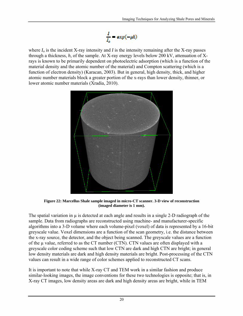
X-ray computed tomography (CT scanning) produces images by measuring the x-ray transmittance of a sample, or the extent to which x-rays will pass through a sample. CT scanning produces 3-D digital reconstructions of a sample by combining numerous 2-D radiographs collected at multiple angles around an object (Figure 22). Medical use of CT scanning for determination of internal maladies by health care professionals was the initial use of this technology in the 1970’s, but very quickly the petroleum industry saw the usefulness of using medical CT scanning to visualize the internal structure of rock cores in the 1980’s (Fujii and Uyama, 2004). CT scanning for quality control in manufacturing has become a more common practice with the advent of industrial CT scanners, which are typically able to obtain images of higher resolution, since no radiation dosage limits need to be adhered to as is the case with living specimens. Though setups vary widely, in general a CT scanner will have an x-ray source located opposite an x-ray detector with the sample to be imaged placed in between the two. Either the source and detector will rotate around the object to be scanned or the scanned object will rotate, typically 360° with tens to thousands of individual x-ray images captured. The density, thickness, and material composition of the sample determine what percentage of the x-rays pass through to the detector. The linear attenuation coefficient µ at each point in the 2-D radiograph is measured by the CT detector. The µ is defined by Beer’s law (Karacan, 2003),


20

where Io is the incident X-ray intensity and I is the intensity remaining after the X-ray passes through a thickness, h, of the sample. At X-ray energy levels below 200 kV, attenuation of X-rays is known to be primarily dependent on photoelectric adsorption (which is a function of the material density and the atomic number of the material) and Compton scattering (which is a function of electron density) (Karacan, 2003). But in general, high density, thick, and higher atomic number materials block a greater portion of the x-rays than lower density, thinner, or lower atomic number materials (Xradia, 2010).

Figure 22: Marcellus Shale sample imaged in micro-CT scanner. 3-D view of reconstruction (imaged diameter is 1 mm).

The spatial variation in µ is detected at each angle and results in a single 2-D radiograph of the sample. Data from radiographs are reconstructed using machine- and manufacturer-specific algorithms into a 3-D volume where each volume-pixel (voxel) of data is represented by a 16-bit greyscale value. Voxel dimensions are a function of the scan geometry, i.e. the distance between the x-ray source, the detector, and the object being scanned. The greyscale values are a function of the µ value, referred to as the CT number (CTN). CTN values are often displayed with a greyscale color coding scheme such that low CTN are dark and high CTN are bright; in general low density materials are dark and high density materials are bright. Post-processing of the CTN values can result in a wide range of color schemes applied to reconstructed CT scans.

It is important to note that while X-ray CT and TEM work in a similar fashion and produce similar-looking images, the image conventions for these two technologies is opposite; that is, in X-ray CT images, low density areas are dark and high density areas are bright, while in TEM


21

images, low density areas are bright and high density areas are dark. Thus, pores in an X-ray CT image will appear very dark or black, while pores in a TEM image will appear very bright or white.

CT scanners have differing maximum resolutions depending on their design. Generally, the maximum image resolution of an instrument and the maximum sample size are inversely proportional. For example, a scanner that can show features as small as a few µm will not be able to scan as large of a sample as a scanner that can only show features as small as a few mm. Common classes of CT scanners include the following (Fujii and Uyama, 2004):

Medical: designed to rotate around a human body (or portion of the human body). Many modern medical CT scanners use fan beams of X-rays and multiple banks of detectors to capture multiple radiograph slices quickly, thus reducing the time of the scan and the amount of radiation to which the human is subjected. The geometry of the scanner and the rapid scanning process results in lower resolution scans than other CT scanning techniques, but it is much faster and ideal for capturing dynamic processes (e.g. flow tests) or data from large amounts of core. A 16 slice Aquillion CT scanner is shown in Figure 23, along with a 2-D slice through the middle of a 3-ft long shale core showing variation of the internal structure in Figure 24.

Figure 23: A 16 slice Aquillion CT scanner.


22

Figure 24: A 2-D slice through the center of a 3-ft long core of Martinsburg Shale. Darker (less dense) bands generally correlate with regions of higher organic matter content in shale

samples. Fine, dark traces represent fractures.

Industrial: designed primarily for quality control of manufactured parts. Smaller systems have a rotating sample stage that enables a CT source and detector to be placed on either side of an object and the sample rotates independently. Larger systems, for quality control on fully assembled vehicles for instance, have fully independent articulating arms that enable the CT source and detector to move around the sample. Within the geosciences, typically smaller systems with rotating sample stages are used. The ability to expose the samples to higher amounts of X-rays with the CT source close to the object and the detector relatively far away results in higher resolution scans than medical CT scanners can provide, but scans typically take much longer. Two photographs of a NorthStar Imaging M-5000 are shown in Figure 25, with the static detector shown on the left and the X-ray source shown on the right. In both images the same 4-in. diameter sandstone core is shown on the rotating sample stage. An example of the scan quality from this type of scanner is shown in Figure 26.

Figure 25: NorthStar Imaging M-5000 industrial CT scanner. Left: X-ray detector with vertical sandstone core. Right: X-ray source with vertical sandstone core.


23

Figure 26: Single slice of data along an XY plane of a reconstructed 1-in. diameter sample of Marcellus Shale with a mineralized fracture intersecting the matrix, scanned with the industrial scanner shown in Figure 25. Scanned diameter is equal to sample diameter.

Micro: Similar to the design of industrial scanners with rotating sample stages, micro CT scanners are high-precision CT scanners that enable small samples to be scanned extremely close to the X-ray source. These systems are designed in enclosures to enable their use inside of laboratories without the need to construct radiation shielding (Figure 27). Samples a few millimeters in diameter are best suited for micro-CT scanners, and can result in reconstructed volumes with a voxel volume of less than 1 cubic micron.

Figure 28 shows a sandstone, with grains and pore space visible, compared with a shale, with compositional differences visible but pores too small to be seen with the micro-CT (note difference in scale bar sizes).

Figure 27: Xradia MicroCT-400 micro CT scanner. Left: Self-contained MicroCT setup with doors open. Right: Close-up of source (left), sample stand with red coffee straw

(center), and various detectors (right).


24

Figure 28: Note that for both samples, the imaged diameter is smaller than the sample diameter. Left: Single slice of data along an XY plane of a reconstructed 6-mm diameter cylindrical sample of calcite-cemented sandstone. Right: Single slice of data along an XY

plane of a reconstructed 4-mm diameter cylindrical sample of Marcellus Shale (Union Springs Member). Dark areas within blue ellipses are organic matter, bright patches are

dense minerals such as calcite and/or pyrite.

Nano: Nanofocus-CT scanners are in many ways the logical advancement of high-resolution scanning that has previously been realized with the evolution of CT scanners from medical to micro CT scanners. Currently there are few of these systems available on the commercial market, and the resolution per pixel ranges from 500 to roughly 50 nm, which at best is about an order of magnitude improvement from the best available micro-CT systems. These systems are similar in design to micro-CT systems, as shown in Figure 29, and have similar limitations and advantages. Nanofocus-CT systems have been used to image microfossils (Figure 30) and have the potential to visualize some of the pore space within shale. However, they are not yet capable of imaging all relevant shale features and require a very small sample size.


25

Figure 29: Left: GE Phoenix Nanotom S nanofocus CT scanner. Right: Segmented pores in a carbonate; sample diameter is 2 mm. Images from GE (2014).

Figure 30: Microfossil scanned in a nano-CT using phase contrast mode to highlight structural details. Image from Sen Sharma (2011).

In addition to scanning uncontained samples, CT scanners can also image rock within core holders. This allows for the control of additional parameters such as pore pressure, confining pressure, temperature, and the addition of fluids. With this extended capability, shale can be imaged at reservoir conditions. Furthermore, by scanning multiple times at different time steps, the results of various treatments can be observed (e.g., before and after saturation with hydraulic fracturing fluid or carbon dioxide, or before and after a pressure change), or dynamic processes


26

can be captured. Figure 31 is an example of the latter, in which brine pushes a slug of methane through a saturated fractured sandstone core.

Figure 31: Time series from medical X-ray CT of brine pushing methane through a saturated fractured Berea Sandstone core, 2-in. diameter. Darkest areas are methane.

Arrow shows flow direction. Left: brine flowing through fracture with no methane present. Left center: pockets of methane flowing through fracture. Right center: decreased bubble size and total volume of methane due to brine flow through fracture. Right: few remaining

bubbles of methane after brine has pushed most methane out of fracture (top: methane remains trapped at inlet).

2.5 ADDITIONAL TOOLS AND ANALYSIS

Three-dimensional reconstructions from X-ray CT, TEM CT, or FIB-SEM sequential imaging can be evaluated quantitatively to determine surface areas, pore volume/porosity, mineral volumes, pore size distribution, relative permeability, or changes in any of these properties. These calculations are often performed with the aid of image analysis software (such as the open-source program ImageJ, or Avizo Fire). Since the pixel values in these images represent relative density or composition, thresholding or selecting specific pixel values, along with cluster analysis, can isolate a desired volume from the rest of the rock volume; these volume amounts can then be compared to determine bulk composition, porosity, or changes in either. Figure 32 shows a 3-D reconstruction of an X-ray CT scan in which minerals and voids have been isolated. More extensive analysis can yield connected porosity, disconnected porosity, pore size distribution, permeability, and relative permeability. X-ray CT and TEM can also be used to quantify changes in any of these properties by subtracting before and after images from one another (i.e., before and after chemical exposure, flow-through, etc.); the same cannot be done with FIB-SEM sequential imaging, as the successive ion milling destroys the original sample


27

area. Dynamic processes, such as fluid flow, that are captured with X-ray CT can also be quantified using these methods.

Figure 32: Martinsburg Shale core scanned in industrial X-ray CT. Left: 3-D view of original reconstruction. Right: Core segmented by density and clustering. Red: fracture

volume. Blue: organic matter. Pink: carbonate. Green: porosity.


28

3. DISCUSSION

The nanometer-scale features of shales present a challenge for viewing grains, pores, and rock fabric using traditional techniques. Traditional optical mineralogy and petrography can be used to examine the general fabric of shales and to identify larger mineral grains, but cannot approach the resolution needed to view pore structures and connectivity. SEM provides significantly improved resolution with the ability to view clay-sized grains, nano-pores, and nano-structures, and produces images based on sample topography and composition. In combination with FIB, SEM can produce 3-D representations of a sample with some interpolation. TEM is also capable of showing nano-scale features, but can further magnify to show angstrom-scale features, with images representing relative density. While SEM images represent the surface or shallow (nm) subsurface of a sample, TEM images display features from the entire thickness of the sample; however, sample thickness is only about 100 nm. X-ray CT also shows features from the entire thickness of the sample, but creates a 3-D reconstruction of the scanned volume in addition to 2-D images. Depending on the resolution and sample size desired, imaging can be completed on samples from several microns in diameter and length to 10 cm in diameter and 3 ft in length. X-ray CT images are based on relative density, similar to TEM, and can show compositional variation and fractures throughout shale. X-ray CT also has the ability to quantitatively analyze dynamic processes, such as fluid flow or structural alteration, by collecting multiple scans over time. SEM and TEM instruments share some additional analytical techniques: diffraction patterns are used to identify crystals and analyze strain, and EDS is commonly used to provide more specific data on elemental composition. The development of TEM CT has the potential to create the most accurate 3-D representation of pore networks in shales, as it has higher resolution than X-ray CT and does not rely on interpolation as FIB-SEM 3-D reconstructions do. As with all analytical techniques, it is helpful to have some idea of the structures, minerals, and features that may be present in a sample before attempting to image it. This allows for any problems or artifacts created by the imaging process to be more easily identified

While the ability to view nano-scale features, particularly pores, is very important to the study of shales, high resolution imaging has scaling limitations. As image resolution increases, sample size generally decreases, creating less certainty that any given sample is truly representative of the larger rock formation. The inherent heterogeneity of rocks, especially across geographic regions, furthers this uncertainty. Imaging a greater number of samples from the formation and member of interest can help increase certainty that features are not anomalous, and can potentially uncover geographic trends in rock characteristics.

As we continue to exploit new unconventional resources and greenhouse gases in the atmosphere continue to increase, understanding the full potential of shales becomes more important to a growing number of scientists. The increased interest in shales over the past several years provides an opportunity to apply new knowledge across research disciplines, as the shale properties that are important to hydrocarbon exploitation are important to carbon storage efforts as well. On a project level, the imaging techniques discussed herein can provide compositional information (both mineralogical and elemental), fabric characterization, pore characterization (size, shape, connectivity, spatial distribution, permeability), grain characterization (size, shape, orientation), and data showing change in any of these. On a disciplinary level, the data and analyses that are possible with these instruments are applicable to a wide range of research areas,


29

including reservoir characterization (hydrocarbon or carbon storage), production and injection optimization, long-term storage effects, and environmental impact assessments.


30



31

4. REFERENCES

Boggs, S.; Krinsley, D. Application of cathodoluminescence imaging to the study of sedimentary rocks; Cambridge University Press, 2006.

Cerchiara, R. R.; Fischione, P. E.; Boccabella, M. F.; Marsh, L. M.; Robins, A. C. Sample Preparation of Oil and Gas Shales for EBSD/EDX and FIB/SEM. Microscopy Society of America, Microscopy and Microanalysis Meeting, Phoenix, AZ, July 29–Aug 2, 2012.

Eastman, H. Petrography of the Marcellus Shale in Well WV6, Monongalia County West Virginia. AAPG Annual Convention and Exhibition, Pittsburgh, PA, May 2013.

Fujii, M.; Uyama, K. Recent advances on X-ray CT. X-ray CT for Geomaterials: Soils, Concrete, Rocks; Otani & Obara, Swets & Zeitlinger, Ed.; 2004; p 3–12.

Gandossi, L. An overview of hydraulic fracturing and other formation stimulation technologies for shale gas production; JRC Technical Report; EUR 26347 EN; European Union Institute for Energy and Transport, Joint Research Center, European Commission, 2013. http://publications.jrc.ec.europa.eu/repository/bitstream/111111111/30129/1/an%20overview%20of%20hydraulic%20fracturing%20and%20other%20stimulation%20technologies%20(2).pdf

GE Measurement & Control. Phoenix Nanotom S: Applications. 2014. http://www.ge-mcs.com/en/radiography-x-ray/ct-computed-tomography/nanotom-s.html

Goldstein, G. I.; Newbury, D. E.; Echlin, P.; Joy, D. C.; Fiori, C.; Lifshin, E. Scanning electron microscopy and x-ray microanalysis; Plenum Press: New York, 1981.

Goldstein, J.; Newbury, D. E.; Joy, D. C.; Lyman, C. E.; Echlin, P.; Lifshin, E.; Sawyer, L.; Michael, J. R. Scanning electron microscopy and X-ray microanalysis; Springer, 2003.

Ishida, T.; Aoyagi, K.; Niwa, T.; Chen, Y.; Murata, S.; Chen, Q.; Nakayama, Y. Acoustic emission monitoring of hydraulic fracturing laboratory experiment with supercritical and liquid CO2. Geophysical Research Letters 2012, 39.

Karacan, C. Ö. Heterogeneous sorption and swelling in a confined and stressed coal during CO2 injection. Energy & Fuels 2003, 17, 1595–1608.

Loucks, R. G.; Reed, R. M.; Ruppel, S. C.; Jarvie, D. M. Morphology, genesis, and distribution of nanometer-scale pores in siliceous mudstones of the Mississippian Barnett Shale. Journal of Sedimentary Research 2009, 79, 848–861.

Loucks, R. G.; Reed, R. M.; Ruppel, S. C.; Hammes, U. Spectrum of pore types and networks in mudrocks and a descriptive classification for matrix-related mudrock pores. AAPG bulletin 2012, 96, 1071–1098.

Nelson, P. H. Pore-throat sizes in sandstones, tight sandstones, and shales. AAPG bulletin 2009, 93, 329–340.


32

Reidenbach, V. G.; Harris, P.C.; Lee, Y. N.; Lord, D. L. Rheological study of foam fracturing fluids using nitrogen and carbon dioxide. SPE Production Engineering 1986, 1, 31–41.

Reimer, L. Scanning electron microscopy: physics of image formation and microanalysis; Springer, 1998.

Salh, R. Silicon Nanocluster in Silicon Dioxide: Cathodoluminescence, Energy Dispersive X-Ray Analysis and Infrared Spectroscopy Studies. Crystalline Silicon - Properties and Uses; = Basu, S., Ed.; InTech, 2011. http://www.intechopen.com/books/crystalline-silicon-properties-and-uses/silicon-nanocluster-in-silicon-dioxide-cathodoluminescence-energy-dispersive-x-ray-analysis-and-infr

Scholle, P. A.; Ulmer-Scholle, D. S. A Color Guide to the Petrography of Carbonate Rocks: Grains, Textures, Porosity, Diagenesis. AAPG Memoir 2003, 77.

Sen Sharma, K. Novel biomedical and biological applications using lab-based multi-scale CT system. Annual Meeting of the Biomedical Engineering Society, Hartford, CT, Oct 2011.

Sondergeld, C. H.; Ambrose, R. J.; Rai, C. S.; Moncrieff, J. Micro-structural studies of gas shales. SPE Unconventional Gas Conference, Society of Petroleum Engineers, 2010.

Tomutsa, L.; Silin, D. B.; Radmilovic, V. Analysis of chalk petrophysical properties by means of submicron-scale pore imaging and modeling. SPE Reservoir Evaluation & Engineering 2007, 10, 285–293.

U.S. Energy Information Administration (EIA). Technically Recoverable Shale Oil and Shale Gas Resources: An Assessment of 137 Shale Formations and 41 Countries Outside the United States; 2013.

Walls, J. D. ; Diaz. E. Relationship of Shale Porosity-Permeability Trends to Pore Type and Organic Content. Denver Well Logging Society, Petrophysics in Tight Oil Workshop, Denver, CO, Oct 26, 2011.

Williams, D. B.; Carter, C. B. Transmission Electron Microscopy: A Textbook for Materials Science; Plenum Press, 2007.

Xradia. MicroXCT-200 and MicroXCT-400 User’s Guide. Version 7.0, Revision 1.5; Apr 2010.

NETL Technical Report Series

Sean Plasynski Director Strategic Center for Coal National Energy Technology Laboratory U.S. Department of Energy Gregory Kawalkin Senior Management & Technical Advisor Strategic Center for Coal National Energy Technology Laboratory U.S. Department of Energy Dan Driscoll Senior Management & Technical Advisor Strategic Center for Coal National Energy Technology Laboratory U.S. Department of Energy Traci Rodosta Carbon Storage Technology Manager Office of Coal & Power Research & Development National Energy Technology Laboratory U.S. Department of Energy

Cynthia Powell Director Office of Research and Development National Energy Technology Laboratory U.S. Department of Energy Kevin Donovan RES Program Manager URS Corporation

Date post:	20-Mar-2018
Category:	Documents
Upload:	hoangdiep
View:	215 times
Download:	1 times

Imaging Techniques for Analyzing Shale Pores and … Library/Research/onsite research...assumes any...

Documents