Imitative Learning for Online Planning inMicrogrids

Samy Aittahar1, Vincent Francois-Lavet1, Stefan Lodeweyckx2,Damien Ernst1, and Raphael Fonteneau1

1 Department of Electrical Engineering and Computer Science,University of Liege, Belgiumsaittahar@student.ulg.ac.be

{v.francois, dernst, raphael.fonteneau }@ulg.ac.behttp://www.montefiore.ulg.ac.be

2 Enervalis,Greenville Campus, Belgium

stefan.lodeweyckx@enervalis.comhttp://www.enervalis.com

Abstract. This paper aims to design an algorithm dedicated to opera-tional planning for microgrids in the challenging case where the scenariosof production and consumption are not known in advance. Using expertknowledge obtained from solving a family of linear programs, we build alearning set for training a decision-making agent. The empirical perfor-mances in terms of Levelized Energy Cost (LEC) of the obtained agentare compared to the expert performances obtained in the case where thescenarios are known in advance. Preliminary results are promising.

Keywords: Machine learning, Planning, Imitative learning, Microgrids

1 Introduction

Nowadays, electricity is distributed among consumers by complex and large elec-trical networks, supplied by conventional power plants. However, due to the dropin the price of photovoltaic panels (PV) over the last years, a business case hasappeared for decentralized energy production. In such a context, microgrids thatare small-scale localized station with electricity production and consumptionhave been developed. The extreme case of this decentralization process consistsin being fully off-grid (i.e. being disconnected from conventional electrical net-works). Such a case requires to be able to provide electricity when needed withinthe microgrid. Since PV production varies with daily and seasonal fluctuations,storage is required to balance production and consumption.

In this paper, we focus on the case of fully off-grid microgrids. Due to the costof batteries, sizing a battery storage capacity so that it can deal with seasonalfluctuations would be too expensive in many parts of the world. To overcomethis problem, we assume that the microgrid is provided with another storagetechnology, whose storage capacity is almost unlimited, such as for example

2 Imitative Learning for Online Planning in Microgrids

as it is the case with hydrogen-based storage. However, this long-term storagecapacity is limited by the power it can exchange.

Balancing the operation of both types of storage systems so as to avoid atbest power cuts is challenging in the case where production and consumption arenot known in advance. The contribution presented in this paper aims to build adecision making agent for planning the operation of both storage systems. To doso, we propose the following methodology. First, we consider a family of scenariosfor which production and consumption are known in advance, which allows us todetermine the optimal planning for each of them using the methodology proposedin [4] which is based on linear programming. This family of solutions is used as anexpert knowledge database, from which optimal decisions can be extracted into alearning set. Such a set is used to train a decision making agent using supervisedlearning, in particular Extremely Randomized Trees [5]. Our supervised learningstrategy provides the agent with some generalization capabilities, which allowsthe agent to take high performance decisions without knowing the scenarios inadvance. It only uses recent observations made within the microgrid.

The outline of this paper is the following. Section (2) provides a formalizationof the microgrid. Section (3) describes the related work. Section (4) introduces alinear programming formalization of microgrid planning with fully-known scenar-ios of production and consumption. Section (5) describes our imitative learningapproach. Section (6) reports and discusses empirical simulations. Section (7)concludes this paper.

2 Microgrids

Microgrids are small structures providing energy available within the systemto loads. The availability of the power strongly depends on the local weatherwith its own short-term and long-term fluctuations. We consider the case wheremicrogrids have both generators and storage systems and also loads. This sectionformally defines such devices. It ends with a definition of Levelized Energy Costwithin a fully off-grid microgrid.

2.1 Generators

Generators convert any source of energy into electricity. They are limited by thepower they can provide to the system. More formally, let us define G as the setof generators, yg as the supply power limit of g ∈ G in Wp and ηg the efficiency,i.e. the percentage of energy available after generation, of g ∈ G and pgt theavailable power from the source of energy. The following inequation describesthe maximal power production:

pgt ηg 6 yg . (1)

In our work, we consider photovoltaic panels, for which the power limitationis linearly dependent of the surface size of the PV panel which is expressed in m2.

Imitative Learning for Online Planning in Microgrids 3

Let xg be the surface size of g ∈ G. The total power production by the surfacesize is expressed as the following equation, for which the constraint expressedabove still holds:

φgt = xgpgt ηg . (2)

2.2 Storage Systems

Storage systems exchange the energy within the system to meet loads demandand possibly to fill other storage systems. They are limited either by capacityor power exchange. We denote these limits by xσc and xσp respectively, whereσc ∈ ΣC , σc ∈ ΣP . We denote Σ = ΣP + ΣC as the set of both kind ofstorage systems and ησ the efficiency of σ ∈ Σ. We consider also, ∀σ ∈ Σ, thevariables sσt for the storage content, a+,σt and a−,σt for the decision variablescorresponding discharge and the recharge amount of the storage system at eachtime t. Dynamics of storage systems are defined by the following equations:

sσs,0 = 0,∀σ ∈ Σ , (3)

sσt = sσ(t−1) − a−,σt−1 − a

+,σ(t−1), 1 6 t 6 T − 1,∀σ ∈ Σ . (4)

2.3 Loads

Loads are expressed in kWh for each time step t. Power cuts occur when thedemand is not met, and the lack is associated with a penalty cost. Formally, wedefine the net demand dt as the difference between the consumption, defined byct and the available energy from the generators. The following equation holds:

dt = ct −∑g∈G

φgt ,∀0 6 t 6 T − 1 . (5)

Finally, Ft is defined as the energy not supplied to loads, expressed in kWh, bythe following equation:

Ft = dt −∑σ∈Σ

ησ(a+,σt + a−,σt ),∀0 6 t 6 T − 1 . (6)

We now introduce in the model the possibility to have several levels of prioritydemand, defined by the cost associated to power cuts. Let Ψ be the set of prioritydemands, and Fψt the number of kWh not supplied for the demand priority groupψ ∈ Ψ . Hence, Equations (5) and (6) become:

dt =∑ψ∈Ψ

cψt −∑g∈G

φgt ,∀0 6 t 6 T − 1 , (7)

∑ψ∈Ψ

Fψt = dt −∑σ∈Σ

ησ(a+,σt + a−,σt ),∀0 6 t 6 T − 1 . (8)

4 Imitative Learning for Online Planning in Microgrids

2.4 Levelized Energy Cost

Any planning of a microgrid given any scenario of production and consumptionleads to a cost based on power cuts and initial investment. It also takes into ac-count economical aspects (e.g. deflation). This cost, called the Levelized EnergyCost (LEC) for a fully off-grid microgrid is formally defined below:

LEC =

∑ny=1

Iy−My

(1+r)y + I0∑ny=1

εy(1+r)y

, (9)

where

– n = Considered horizon of the system in years;– Iy = Investments expenditures in the year y;– My = Operational revenues performed on the microgrid in the year y (take

into account the cost of power cuts during the year y);– εy = Electricity consumption in year y;– r = Discount rate which may refer to the interest rate or discounted cash

flow.

3 Related Work

Different steps of our contribution have already been considered in various appli-cations. We used linear programming for computing expert strategies. This kindof approach have already been discussed in [8], [9] and [7] with different microgridformulations. We used supervised learning techniques with solutions provided bylinear programming. Cornelusse et al. [2] have considered this approach in theunit commitment problem. Our prediction model needs an additional step toensure compliance of the policy learned by supervised learning algorithms withconstraints related to the system. This step consists to use quadratic program-ming to postprocess the solution. Cornelusse et al. [1] have considered a similarapproach.

Online planning for microgrids has also been studied with others microgridconfigurations. For example, Debjyoti and Ambarnath [3] focuses on the specificcase of online planning using automatas, while Kuznetsova et al. [6] focuses onthe online planning using a model-based reinforcement learning approach.

4 Optimal Sizing and Planning

4.1 Linear program

Objective function Let kψt ,∀0 6 t 6 T − 1,∀ψ ∈ Ψ be the value of loss load ofthe priority demand ψ ∈ Ψ . The LEC is instantiated in the following way:

Imitative Learning for Online Planning in Microgrids 5

LEC =

∑Tt=1

−∑ψ∈Ψ k

ψt F

ψt

(1+r)y′+ I0∑n

y=1εy

(1+r)y, (10)

where y′ = t/(24× 365).

Constraints Storage systems actions are limited by their sizes. The followingconstraints are added:

sσct 6 xσc ,∀σc ∈ ΣC , 0 6 t 6 T − 1 , (11)

a+,σpt 6 xσp ,∀σp ∈ ΣP , 0 6 t 6 T − 1 , (12)

−a−,σpt 6 xσp ,∀σp ∈ ΣP , 0 6 t 6 T − 1 . (13)

Figure (1) shows the overall linear program.

Min.

∑Tt=1

−∑ψ∈Ψ k

ψt F

ψt

(1+r)y + I0∑ny=1

εy(1+r)y

, y = t/(365× 24) (14a)

S.t., ∀t ∈ {0 . . . T − 1} : (14b)

sσt = sσt−1 + a−,σt−1 + a+,σt−1,∀σ ∈ Σ , (14c)

sσct 6 xσc ,∀σc ∈ ΣC , (14d)

a+,σpt 6 xσp ,∀σp ∈ ΣP , (14e)

a−,σpt 6 xσp ,∀σp ∈ ΣP , (14f)∑ψ∈Ψ

Fψt 6 −dt −∑σ∈Σ

ησ(a−,σt + a+,σt ) , (14g)

∑ψ∈Ψ

Fψt 6 0 , (14h)

− Fψt 6 cψt . (14i)

Fig. 1. Overall linear program for optimization.

4.2 Microgrid Sequence

When planning is performed given sequences of production and consumptionof length T > 0, a sequence of storage contents and a sequence of actions are

6 Imitative Learning for Online Planning in Microgrids

generated. Such a group of four sequences is called a microgrid sequence. Inthe following, we abusively denote as an optimal microgrid sequence a set ofsequences obtained by solving linear programs. Figure (2) shows an illustrationof a sequence of decision, with the two kinds of storage systems. A microgridsequence is formally defined below:

(c0 . . . cT−1, φ0 . . . φ0...T−1, sσ0 . . . s

σT−1, a

σ0 . . . a

σT−1) , (15)

where ∀t ∈ {0 . . . T − 1}, aσt = a+,σt + a−,σt .

Fig. 2. Sequence scheme (discharging/recharging).

The cost associated to a microgrid sequence is defined below for any microgridsequence s given any microgrid configuration M , any sequence of productionφ0...T−1 and any sequence of consumption c0...T−1:

LECc0...cT−1,φ0...φT−1

M (s) =

∑Tt=1

−∑ψ∈Ψ k

ψt ((ct−

∑g∈G φ

gt )−

∑σ∈Σ η

σ(a+,σt +a−,σt ))

(1+r)y′+ I0∑n

y=1εy

(1+r)y.

(16)

5 Imitative Learning approach

Optimal microgrid sequences are generated as an expert knowledge database.The decision-making agent is built using a subset of this database. Such anagent is evaluated on a distinct subset.

5.1 Data

Given production and consumption sequences, we can generate microgrid se-quences by solving linear programs.

Imitative Learning for Online Planning in Microgrids 7

Formally, let (φ(k)t , c

(k)t )t∈{0...T−1},k∈{0...K} be a set of production and con-

sumption scenarios, with K ∈ N\0. To this set corresponds a set of microgridsequences:

(φ(k)t , c

(k)t , s

(k,σ)t , a

(k,σ)t )k∈K,t∈{0,...,T−1} . (17)

5.2 From Data to Feature Space

For each time t ∈ {0, . . . , T − 1}, production and consumption data are known

from 0 to t. Let φ(k)0...t =

⟨φ(k)0 . . . φ

(k)t

⟩and c

(k)0...t =

⟨c(k)0 . . . c

(k)t

⟩be the sequences

of production and consumption from 0 to t. We define a microgrid vector fromthe previous sequences:

(φ(k)0...t, c

(k)0...t, s

(k,σ)t , a

(k,σ)t )k∈K,t∈{0...T−1},∀σ∈Σ . (18)

We now introduce, ∀t ∈ {0 . . . T − 1}, the function e : Rt × Rt × Rbt → Rbtwhere b = #Σ. Such a function builds an information vector from sequences of

production and consumption. Let v = e(φ(k)0...t, c

(k)0...t) be the information vector,

vl the l-th component of v and L > 0 the size of the vector. Finally we define,from the definition of microgrid vector, a feature space that will be used withsupervised learning techniques as below:

(v1 . . . vL, s(k,σ)t , a

(k,σ)t )k∈K,t∈{0...T−1},∀σ∈Σ . (19)

5.3 Constraints Compliancy

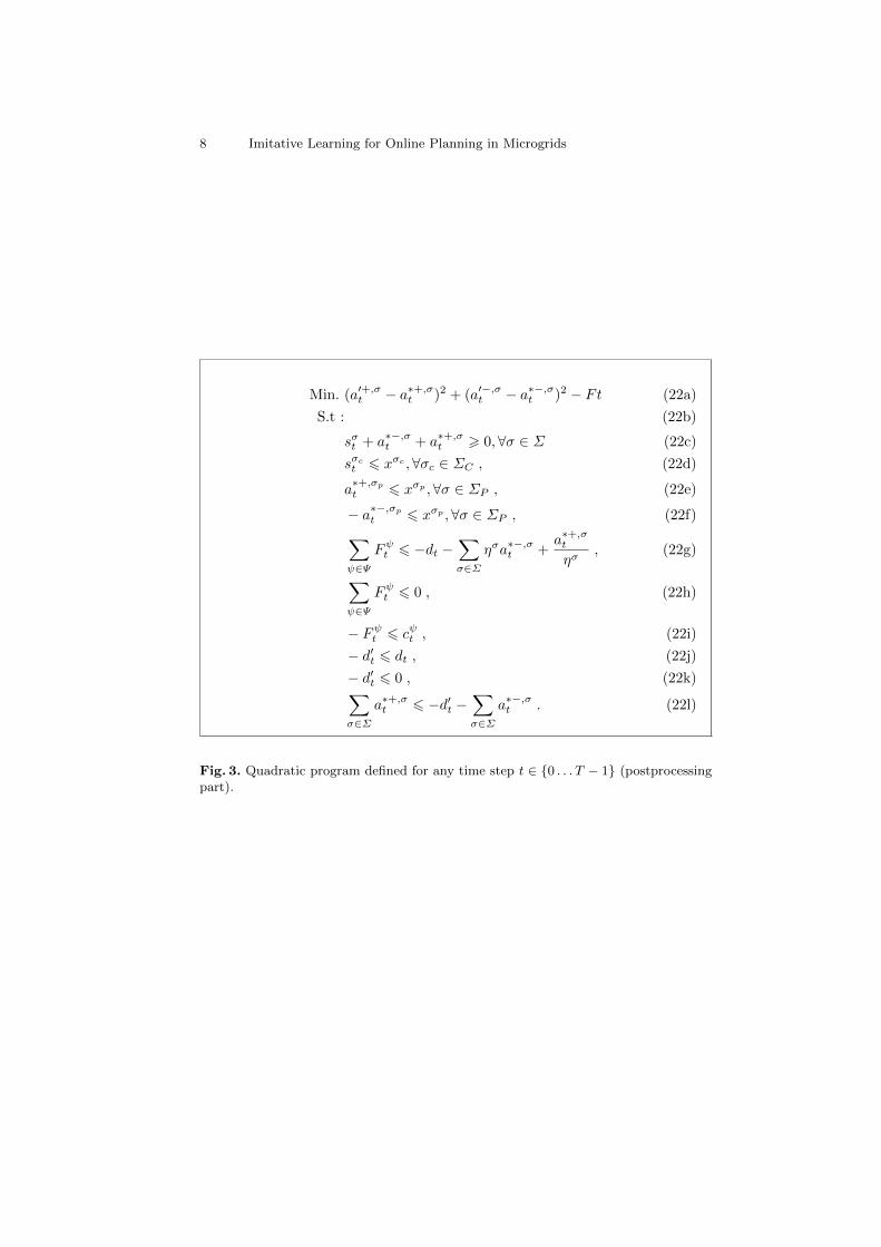
An additional step is to ensure that the constraints related to the current infor-mation of the system are not violated with the actions performed by the decisionmaking agent. A quadratic program is designed to search for closest feasible ac-tions. This program is defined in Figure (3). We use constraints from Figure (1)with an extra one defined below which represents the limit of storage systemrecharging regarding the overall available energy in the system.∑

σ∈Σa∗+,σt 6 −d′t −

∑σ∈Σ

a∗−,σt , (20)

where d′t is defined below to take into account only the possible overproductionby the following equation:

d′t = −max(0, dt) . (21)

We are going to illustrate the postprocessing part (see also Figure (4)). Wewill consider three use cases below, with a battery limited in capacity by 11kWhand a hydrogen tank with a power exchange limit of 7kWp.

– Underproduction with both storage systems empty. Initial actions are bothdischarging but since this is not possible, the postprocessing part cancels theactions (Figure (4) - top);

8 Imitative Learning for Online Planning in Microgrids

Min. (a′+,σt − a∗+,σt )2 + (a′−,σt − a∗−,σt )2 − Ft (22a)

S.t : (22b)

sσt + a∗−,σt + a∗+,σt > 0,∀σ ∈ Σ (22c)

sσct 6 xσc ,∀σc ∈ ΣC , (22d)

a∗+,σpt 6 xσp ,∀σ ∈ ΣP , (22e)

− a∗−,σpt 6 xσp ,∀σ ∈ ΣP , (22f)∑ψ∈Ψ

Fψt 6 −dt −∑σ∈Σ

ησa∗−,σt +a∗+,σt

ησ, (22g)

∑ψ∈Ψ

Fψt 6 0 , (22h)

− Fψt 6 cψt , (22i)

− d′t 6 dt , (22j)

− d′t 6 0 , (22k)∑σ∈Σ

a∗+,σt 6 −d′t −∑σ∈Σ

a∗−,σt . (22l)

Fig. 3. Quadratic program defined for any time step t ∈ {0 . . . T − 1} (postprocessingpart).

Imitative Learning for Online Planning in Microgrids 9

– Overproduction with hydrogen tank empty and battery containing 7kWh.Initial actions are both charging. But the production itself does not entirelymeet the consumption. Again, there is a projection where only the batteryis discharging (Figure (4) - middle);

– Underproduction with both storage systems are not empty. The actions areboth charging but the energy requested does not meet entirely the consump-tion. As a consequence, the levels of charging of the battery and of thehydrogen tank are decreased by the projection (Figure (4) - bottom).

5.4 Evaluation

An evaluation criterion consists to compute the difference of cost observed be-tween control by the imitative agent and the optimally control microgrid, fora given context (i.e. profile of production/consumption and microgrid settings).More formally, let’s consider s∗ the optimal microgrid sequence and s′ the micro-grid sequence generated by the decision making agent. Then the cost differenceis represented by the function below:

Errc0...cT−1,φ0...φT−1

M (s′) = LECc0...cT−1,φ0...φT−1M (s′)−LECc0...cT−1,φ0...φT−1

M (s∗) .(23)

6 Simulations

6.1 Implementation Details

The programming language Python3 was used for all the simulations, with thelibrary Gurobi4 for optimization tools and scikit-learn5 for machine learningtools.

6.2 Microgrid Components

Devices below are considered for the microgrid configuration.

– Photovoltaic panels accumulate energy from solar irradiance with a ratio ofloss due to technology and atmospheric issues. According to Section (2), theyare defined in terms of m2 and of Wp per m2. Table (1) gives the values ofthe elements describing the PV panels.

– Batteries are considered as short-term storage systems with no constrainton power exchange but with limited capacity. Table (2) gives the values ofthe elements describing the batteries.

– Hydrogen tanks, without capacity constraint, but limited in power exchange.They are long-term storage systems. Table (3) gives the values of the ele-ments describing the hydrogen tanks.

3 www.python.org4 http://www.gurobi.com/5 www.scikit-learn.org

10 Imitative Learning for Online Planning in Microgrids

Fig. 4. Bar plots representing the projection from actions to feasible ones when needed.

Table 1. Photovoltaic panels settings.

Efficiency ηPV 20%Cost by m2 200 eWp/m2 200Lifetime 20 years

Imitative Learning for Online Planning in Microgrids 11

Table 2. Batteries settings.

Efficiency charging/discharging ηB 90%Cost per usable kWh 500 eLifetime 20 years

Table 3. Hydrogen tank settings.

Efficiency charging/discharging ηB 65%Cost per kWp 14 eLifetime 20 years

6.3 Available Data

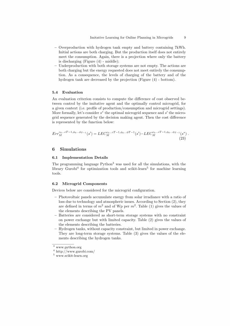
Consumption Profile An arbitrarily pattern was designed as a representativemodel of a common residential daily consumption with two peaks of respectively1200 and 1750 W. Figure (5) shows the daily graph of such a consumption profile.

Fig. 5. Residential consumption profile.

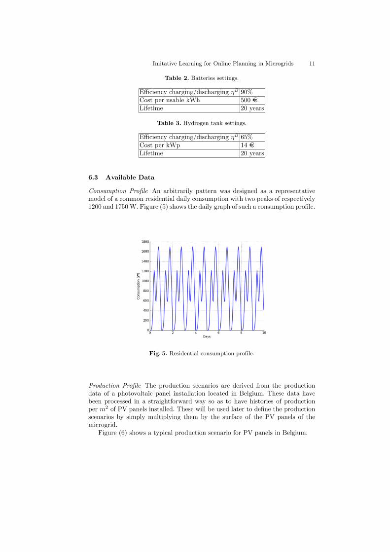
Production Profile The production scenarios are derived from the productiondata of a photovoltaic panel installation located in Belgium. These data havebeen processed in a straightforward way so as to have histories of productionper m2 of PV panels installed. These will be used later to define the productionscenarios by simply multiplying them by the surface of the PV panels of themicrogrid.

Figure (6) shows a typical production scenario for PV panels in Belgium.

12 Imitative Learning for Online Planning in Microgrids

Fig. 6. Monthly production profile of PV panels in Belgium.

6.4 Test Protocol

We split the set of scenarios of production and consumption into two subsets, alearning set for training the agent and a test set to evaluate the performances.The learning set contains the two first years of production and the test setcontains the last year of production. We also apply linear transformations asbelow to artificially create more scenarios for both learning and test sets.⋃

i∈{0.9,1,1.1}

⋃j∈{0.9,1,1.1}

{(ict, jφt)}, t ∈ {0 . . . T − 1} . (24)

Table (4) details the configuration of our microgrid.

Table 4. Microgrid configuration.

Photovoltaic panels area (in m2) 42Battery capacity (in kWh) 13Hydrogen network available power (in kWp) 1

The following information vectors have been considered, ∀t ∈ {0 . . . T − 1}:

– 12 hours of history, i.e. e(φ(k)0 . . . φ

(k)t , c

(k)0 . . . c

(k)t ) =

(φ(k)max(t−12,0) . . . φ

(k)t , c

(k)max(t−12,0) . . . c

(k)t );

– 3 months of history, i.e. e(φ(k)0 . . . φ

(k)t , c

(k)0 . . . c

(k)t ) =

(φ(k)max(t−24×30×3,0) . . . φ

(k)t , c

(k)max(t−2160,0) . . . c

(k)t );

Imitative Learning for Online Planning in Microgrids 13

Fig. 7. Sample of typical Belgium production (1 year).

– 12 hours of history + summer equinox distance, i.e.

e(φ(k)0 . . . φ

(k)t , c

(k)0 . . . c

(k)t ) = (φ

(k)max(t−12,0) . . . φ

(k)t , c

(k)max(t−12,0) . . . c

(k)t , |t−t∗|),

where t∗ is the summer equinox datetime.

A forest of 250 trees have been built with the method of Extremely Random-ized Trees proposed in [5]. Our imitative learning agent and our optimal agentare also compared with a so-called greedy agent that behaves in the followingway.

– If dt > 0, i.e. if underproduction occurs, storage systems are discharged indecreasing order of efficiency;

– If dt 6 0, i.e. if overproduction occurs, storage systems are charged in de-creasing order of efficiency.

The main idea of this greedy agent is to keep as most as possible energy intothe system.

6.5 Results and Discussion

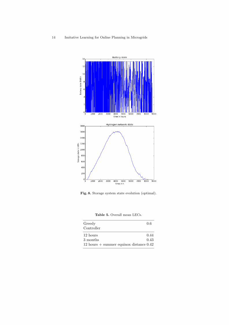
Optimal Sequence of Actions. Figure (8) shows the evolution of the storagesystems contents given optimal sequences of actions, for a given scenario. Theempirical mean LEC over the test set is 0.32e/kWh. The evolution is plottedover 1 year.

As expected, the battery tries to handle short-term fluctuations. On theother hand, the hydrogen tank content gradually increases during summer beforegradually decreasing during winter.

Greedy and Agent-Based Sequences of Actions. Table (6.5) shows the LEC forall the sequences generated by the greedy algorithm and the controller givenseveral input spaces.

14 Imitative Learning for Online Planning in Microgrids

Fig. 8. Storage system state evolution (optimal).

Table 5. Overall mean LECs.

Greedy 0.6Controller

12 hours 0.443 months 0.4312 hours + summer equinox distance 0.42

Imitative Learning for Online Planning in Microgrids 15

Considering a history of production and consumption of only 12 hours is moreexpensive in terms of LEC, compared to a history of production and consumptionof 3 months. It shows that a decision making agent is more efficient with long-term information. Additionally, we also report experimental results for which theagent was also provided with the distance (in time) to summer equinox. Thisadditional information improves the performances.

7 Conclusion

In this paper, we have proposed an imitative learning-based agent for operat-ing both long-term and short-term storage systems in microgrids. The learningset was obtained by solving a family of linear programs, each of them beingassociated with a fixed production and consumption scenario.

As having access to real data is expensive, we plan to investigate how totransfer knowledge from one microgrid to another. In particular, we will focuson transfer learning strategies [11].

Acknowledgments. Raphael Fonteneau is a Postdoctoral Fellow of the F.R.S.-FNRS. The authors also thank the Walloon Region who has funded this researchin the context of the BATWAL project. The authors also thank Bertrand Cor-nelusse for valuable discussions.

Bibliography

[1] Cornelusse, B., Geurts, P., Wehenkel, L.: Tree based ensemble models reg-ularization by convex optimization. In: OPT 2009, 2nd NIPS Workshop onOptimization for Machine Learning (2009)

[2] Cornelusse, B., Vignal, G., Defourny, B., Wehenkel, L.: Supervised learningof intra-daily recourse strategies for generation management under uncer-tainties. In: PowerTech, 2009 IEEE Bucharest. pp. 1–8. IEEE (2009)

[3] Debjyoti, P., Ambarnath, B.: Control of storage devices in a microgrid usinghybrid control and machine learning. In: IET MFIIS 2013, KOLKATA,INDIA, ISBN: 978-93-82715-97-9(online) pg.-5:34 (2013)

[4] Francois-Lavet, V., Gemine, Q., Ernst, D., Fonteneau, R.: Towards the min-imization of the levelized energy costs of microgrids using both long-termand short-term storage devices. To be published (2015)

[5] Geurts, P., Ernst, D., Wehenkel, L.: Extremely randomized trees. MachineLearning 63(1), 3–42 (Apr 2006)

[6] Kuznetsova, E., Li, Y.F., Ruiz, C., Zio, E., Ault, G., Bell, K.: Reinforcementlearning for microgrid energy management. Energy 59, 133–146 (2013)

[7] Moghaddam, A.A., Alireza, S., Niknam, T., Reza Alizadeh Pahlavani, M.:Multi-objective operation management of a renewable {MG} (micro-grid)with back-up micro-turbine/fuel cell/battery hybrid power source. Energy36(11), 6490 – 6507 (2011)

[8] Morais, H., Kdr, P., Faria, P., A Vale, Z., Khodr, H.: Optimal scheduling ofa renewable micro-grid in an isolated load area using mixed-integer linearprogramming. Renewable Energy 35(1), 151 – 156 (2010)

[9] Motevasel, M., Reza Seifi, A., Niknam, T.: Multi-objective energy manage-ment of {CHP} (combined heat and power)-based micro-grid. Energy 51(0),123 – 136 (2013)

[10] Niknam, T., Azizipanah-Abarghooee, R., Rasoul Narimani, M.: An efficientscenario-based stochastic programming framework for multi-objective opti-mal micro-grid operation. Applied Energy 99(0), 455 – 470 (2012)

[11] Pan, S.J., Yang, Q.: A survey on transfer learning. Knowledge and DataEngineering, IEEE Transactions on 22(10), 1345–1359 (2010)