Immersed Boundary Methods for Fluid-Structure Interaction ...€¦ · Optimization within an...

Immersed Boundary Methods forFluid-Structure Interaction and ShapeOptimization within an FEM-based PDEToolbox

Janos Benk, Hans-Joachim Bungartz, Miriam Mehl, and Michael Ulbrich

Abstract One of the main challenges in a classical mesh-based FEM-approachis the representation of complex geometries. This challenge is often tackled by acomputationally costly mesh generation process, where the resulting mesh’s facetsrepresent the boundary. An alternative approach, that we employ here, is the im-mersed boundary (IB) approach. This uses instead a computationally cheaper struc-tured adaptive Cartesian mesh and an explicit boundary representation, where thechallenge mainly lies in the boundary condition (BC) imposition on the mesh cellsintersected by the geometry’s boundary. One IB method is Nitsche’s method that weemploy here for fluid-structure interaction (FSI) and shape optimization problems.The simulation of such complex physical systems modeled by PDEs requires a com-bination of sophisticated numerical methods. Implementing a FEM-based simula-tion software that computes a particular PDE’s solution often requires the reusage ofexisting methods. In order to make our approach public and also to prove the mod-ularity of it, we integrated our IB methods in an existing FEM-based PDE toolboxof the Trilinos project, called Sundance.

Janos BenkComputer Science, Technische Universitat Munchen, Boltzmannstr. 3, 85748 Garching, Germanye-mail: [email protected]

Hans-Joachim BungartzComputer Science, Technische Universitat Munchen, Boltzmannstr. 3, 85748 Garching, Germanye-mail: [email protected]

Miriam MehlInstitute for Advanced Study, Technische Universitat Munchen, Lichtenbergstr. 2a, 85748 Garch-ing, Germany e-mail: [email protected]

Michael UlbrichMathematics, Technische Universitat Munchen, Boltzmannstr. 3, 85748 Garching, Germany e-mail: [email protected]

1

2 J. Benk, H.-J. Bungartz, M. Mehl, M. Ulbrich

1 Introduction

The idea behind the development of a finite element PDE toolbox suitable not onlyfor simulation but also optimization algorithms is to provide a software allowingfor the reuse of mesh functionality, data processing, matrix assembly, linear andnon-linear solvers for various kinds of PDE based applications. To establish a newapplication code, the user only has to provide a suitable formulation of the continu-ous equations and of the finite element basis. Sundance [27, 28] has been developedwith exactly that task. The user implements the particular application in a weak formformulation. This makes also the implementation of dual equations for optimizationvery convenient. In addition to the problem formulation, the type of finite elementbasis to be used has to be prescribed – of course in close connection with the compu-tational grid and, therewith, the element type. Element quadrature, matrix assembly,and (non-)linear solvers are given by Sundance or Trilinos [20], respectively.

The focus of this paper is on the numerical simulation of fluid-structure interac-tion processes and related optimization problems. These problems require the flex-ible handling of complex and moving geometries including large geometrical oreven topological changes. In particular for optimization, a high computational andmemory efficiency is additionally required. Based on these requirements, we addeda further grid type to the Sundance toolbox: structured adaptively refined Cartesiangrids. Due to its strict structuredness, this grid type makes the storage of any explicitstructure information such as relations between vertices, edges, faces, and elementsor between elements and their neighbours obsolete and, thus, reduces the storagerequirements to a minimum.

However, a major drawback of Cartesian grids is their inherently poor approxi-mation accuracy for complex geometries. Thus, sophisticated methods to improvethis accuracy are required. Here, immersed boundary methods such as Nitsche’smethod are a promising approach. In this paper, we present a Cartesian grid im-plementation in Sundance including an extension of Nitsche’s method to flow sim-ulations on moving geometries, in particular fluid-structure interaction and shapeoptimization problems.

In the following section, we show the underlying equations of our fluid-structurescenarios and recall some basic methods for PDE constraint optimization. Sect. 3gives a an overview of immersed boundary methods and the related terminology.In Sect. 4, we shortly introduce the Sundance toolbox with its basic functionality,user interface, and implementational concept. We explain the Cartesian grid imple-mentation in Sect. 5 and introduce Nitsche’s method for fluid dynamics in movinggeometries (Sect. 6). Section 7 presents details on the implementation in Sundance,whereas numerical examples for fluid-structure interactions using Nitsche’s methodand their results are shown in Sect. 8. For shape optimization, we present first simplescenarios with results in Sect. 9. Finally, we summarize results and give an outlookon future work in the conclusion (Sect. 10).

Immersed Boundary Methods for Fluid-Structure Interaction and Shape Optimization 3

2 The Fluid-Structure Interaction Model and OptimizationMethods

The Fluid-Structure Interaction Model. For the simulation of fluid-structure in-teractions on Cartesian grids, we use the incompressible laminar Navier-Stokesequations

∂v∂ t

= ν∆v− (v ·∇)v−∇p+ f f (momentum equation), (1)

∇ ·v = 0 (continuity equation) (2)

to model the fluid flow in connection with the structural dynamics equations

ρs∂ 2u∂ t2 +∇ ·σs + fs = 0, (structural dynamics) (3)

where v denotes the flow velocities, p the fluid pressure, f f external forces acting onthe fluid such as gravity forces, and ν the viscosity of the considered fluid. Further,u is the structure displacement vector, ρS the structure density, σs the stress tensor,and fs denotes external traction forces exerted on the structure.

The interaction between fluid and structure is given by the continuity of velocitiesand the balance of forces

v =∂u∂ t

, (4)

σ f n f = σsns, (5)

where σ f and σs are the stress tensors of fluid and structure and n f and ns denotethe normal vectors of the fluid and structure domain boundaries.

The structure is usually simulated in a Lagrangian framework, i.e., the grid de-forms with the structure movement, such that the surface of the structure is alwaysrepresented accurately. For the fluid domain, we, however, use an Eulerian fixed gridsetting to allow also for large geometry or even topology changes.

Shape Optimization Methods. In our example applications, we consider de-signing the shape of a body B exposed to Navier-Stokes flow such that a givencost functional is minimized. We denote this functional with J(y,Ω) (e.g., the drag)under the constraints EΩ (y) = 0 (Navier-Stokes equations including boundary con-ditions), where y = (v, p) denotes the flow variables and Ω is the fluid domain sur-rounding the body to be optimized. Additional constraints such as constant volumeof the body shape or smoothness of the body’s boundary ensure the existence of anoptimal design. A particular challenge of shape optimization is the fact that duringthe iterative process of optimization a sequence of different domains Ωk is generatedand the PDE has to be solved on each of these changing domains. This is closelyrelated to boundary movement due to structure deformation in the fluid-structureinteraction applications described above.


For gradient-based optimization, the derivative of j(Ω) := J(y(Ω),Ω) with re-spect to domain variations Ω 7→ (Id+V )(Ω) is required, where V is a displacementfield and Id the identity operator.

A classical approach, the method of mappings [6, 18, 33], works with a refer-ence domain Ωref and bi-Lipschitz transformations T : Rn → Rn to represent thecurrent domain via T as Ω = T (Ωref). Using this transformation, the problem canbe transported to the fixed domain Ωref. This results in a nonlinear PDE constrainedoptimal control problem with T serving as the control (design parameterization). Ifpreferred, it can be arranged that the k-th optimization iteration performs its com-putations on the current domain Ωk by viewing it as the reference domain. For con-ventional FEM, this requires moving the computational mesh as well as remeshingif the moved mesh deteriorates.

A closely related alternative to the method of mappings is provided by shapedifferential calculus [42, 47]. It offers a rich machinery for computing the directionalderivative d j(Ω)[V ] := d

dt j((Id+ tV )(Ω))∣∣t=0, called shape derivative if it exists in

the Gateaux sense, in the displacement direction V . The Hadamard-Zolesio structuretheorem [42, 47] states that under suitable conditions there exists a distribution g onthe boundary of Ω such that d j(Ω)[V ] = 〈g,V ·n〉∂Ω . The distribution g representsthe sensitivity of j(Ω) with respect to normal boundary variations. It can be usedto develop shape optimization algorithms that move the boundary of Ω to achieve adescent method.

The shape gradient g or a discrete version of it can be obtained by the adjointapproach [21]. In contrast to the sensitivity method, the computational complexityof the adjoint approach is independent of the dimension of the considered space ofboundary displacement directions V . It requires to compute the adjoint state. If wedenote by u the state and abbreviate the PDE as E(u,Ω) = 0, then the adjoint statew solves the adjoint PDE

(Eu(u,Ω)v,w) =−(Ju(u,Ω),v) ∀ v ∈U0, (6)

where U0 is the space of state variations and the subscript denotes the partial Frechetderivative of the respective operator or function.

3 Immersed Boundary Methods – A Short Overview

The term immersed boundary methods summarizes a class of methods aiming at theaccurate description of complex and moving geometries in a fixed Cartesian grid. Itwas developed already in the seventies by Peskin [37] for the simulation of bloodflow in the human heart. The basic idea is to embed a moving structure in a fluidflow simulated on a fixed (Eulerian) Cartesian grid. The influence of the structureon the flow is taken into account by a force function (which is zero away from thestructure). A good overview on immersed boundary methods is given in [30].


In literature, there exists a variety of methods and a lot of names besides im-mersed boundaries that are related to the same topic: handling complex and movinggeometries in fixed and mostly Cartesian grids. We shortly mention and classify themost important ones:

Marker-and-Cell. Early marker-and-cell methods, introduced by Harlow andWelch already in the sixties [19]) use cell-markes to defined fluid and non-fluid cellsin a free surface flow. This approach obviously can easily be extended to complexflow geometries with obstacles [16] and to fluid-structure interaction [11]. However,the accuracy is restricted by the character of the grid, i.e., for Cartesian grids to O(h)if h is the mesh width.

Volume-of-Fluid. To increase accuracy, volume-of-fluid methods have been in-troduced by Noh and Woodward in 1976 [35]. Instead of simply assigning cells thevalues zero for an empty cell and one for a cell completely filled with fluid, thevolume-of-fluid method introduces a fractial function giving the fraction (in termsof volume) of a grid cell which is filled with fluid. This method has the advantage toallow a fulfillment of mass conservation. The accuracy of the actual geometry rep-resentation is only first order for the original method, but can be enhanced to secondorder (see, e.g., [38]).

Level-Set. To overcome the drawbacks of the volume-of-fluid method, anothertwelve years later, Osher and Sethian introduced the level-set method that tracksthe fluid surface using a function that is zero at the domain boundary (and positiveinside the flow domain) [36]. This allows even for topology changes in a naturalway, conserves mass if applied correctly, and allows for high order of accuracy. Thetransient computation of the level-set function requires the solution of a Hamilton-Jacobi equation, which is neither trivial nor computationally cheap. The fractialfunction of the volume-of-fluid method can be interpreted as a volume integral overthe level-set function.

Cut Cell. In contrast to the aforementioned approaches, cut cell methods [26]work with an explicit representation of the domain boundary by, e.g., polygons in2D, triangulations in 3D, or higher-order surface representation with splines, forexample. Classical cut cell methods use a finite volume discretization on the result-ing geometry consisting of ’standard volumes’ and ’cut cell volumes’. Accordingly,the roots of cut cell methods come from flow simulation. The accuracy depends onthe accuracy of the boundary representation. A drawbacks of the cut cell methodin particular in 3D is the large variety of possible types of cuts through a cell, and,therewith, the large number of different cut cell types. The advtantage is the easygeometry representation with straightforward possibilities to interface with CAD(Computer Aided Design), e.g.

Fictitious Domain. Also fictitious domain methods [10] have been developedoriginally for fluid dynamics but are applied as well for structural dynamics [39].The complex geometry is embedded in a simpler domain such as a square in 2Dor a cube in 3D, and the original equation is replaced by an equation on this sim-pler domain by introducing jumping coefficients. These jumping coefficients can be


interpreted as an extremely high or low stiffness outside the actual domain if thedomain is surrounded by a rigid body or vacuum, e.g.. The resulting system can bediscretized either by finite differences, finite volumes, or finite elements. The draw-back of the fictitious domain method in this simple form is that it allows only themodeling of rather simple boundary conditions such as homogeneous Dirichlet orNeumann boundary conditions. As soon as other boundary conditions such as thoseoriginating from a constant movement of a rigid body in a fluid have to be applied,additional efforts are required such as adding a Lagrange multiplier to enforce theboundary condition (see, e.g., [15]). The accuracy is limited by the accuracy of thediscrete representation of the location of coeffcient jumps as well as the influenceof averaging effects when discretizing the underlying PDE at such a jump.

Penalty Methods. The penalty method proposed by Babuska in the late sixtiesand early seventies [1, 2] for the Poisson equation with homogeneous boundaryconditions allows to weakly enforce boundary conditions with a finite element basisthat is not conforming with these boundary conditions. It enhances the energy func-tional to be minimized by the finite element solution by a boundary penalty termh−s ∫

∂ΩvsdS. In case of a partial differential equation L(u) = f with a differential

operator L, this gives:

F(v) =∫

Ω

L(v)v−2 f vdΩ +h−s∫

∂Ω

vsdS. (7)

This methods performs well in practice. One can be shown to be sensitive withrespect to the choice of s and to deteriorate the order of convergence of the originaldiscretization in theory.

Nitsche’s Method. Nitsche developed a closely related method [34], that also en-hances the energy functional in a finite element setting by a boundary penalty term,but adds further terms ensuring the symmetry of the resulting discrete equationsand, therewith ensures full consistency. Nitsche’s method has been applied to com-putational fluid dynamics in [4] and [3]. In the latter, the method is called weaklyenforced boundary conditions.

Extended Finite Elements. In contrast to penalty and Nitsche’s methods, ex-tended finite element methods [31] enhance the finite element basis (enriched basisfunctions) at sharp internal boundaries, where discontinuities in material proper-ties or cracks cause discontinuities in the numerical solution of a partial differentialequation.

In this paper, we describe an extension of Nitsche’s method for transient prob-lems with moving boundaries (Sect. 6). This is new and requires some additionaltechniques to ensure the numerical stability of the time-stepping scheme.


4 The Sundance Toolbox in a Nutshell

The Sundance toolbox is a convenient software providing the user with a vast func-tionality for several pieces of the so-called simulation pipeline: problem formula-tion, i.e., mesh generation and weak form formulation of the required partial dif-ferential equations, discretization including assembling of a finite element matrix,computation of element matrices and stiffness matrix assembly, and, finally, solversfor the resulting systems of linear or nonlinear discrete equations. Figure 1 showsthe steps of the simulation pipeline and outlines the contributions from users, Sun-dance components and external software components are linked to Sundance viawell-defined interfaces.

Fig. 1 Steps of the simulation pipeline in Sundance. Functionalities provided by Sundance aremarked light blue, functionalities provided both by Sundance and by interfaces to external toolsare green, and functionalities provided exclusively by interfaces to external software are markedred.

A computational grid in Sundance is considered as a collection of mesh entities(elements, faces, edges, vertices) and their relations. A mesh compatible with theSundance interface has to provide the following functionalities:

1. return the unique identification number and dimensionality (0 for vertices, 1 foredges, 2 for faces, 3 for 3D elements) of a mesh entity,

2. return the position, i.e., the spatial coordinates of a given vertex,3. return all lower-dimensional components of a mesh entity, e.g., all faces, edges,

and vertices of a three- dimensional element,4. return the indices of all mesh elements that contain a given mesh entity together

with its indices within the respective elements.

The grid can either be generated by an external mesh generator and read viaa Sundance compatible parser from an input file or be generated internally withinSundance given the characteristic parameters of the mesh. Whereas the first ap-proach is very well suited for unstructured grids and assures a high flexibility withrespect to geometry and mesh generation with existing user-trusted tools, the latter


is more suited for grids with a fixed structure such as our Cartesian grids. The meshfunctionality described above can be either implemented by getting the required in-formation from stored data (as for unstructured grids) or deriving information fromthe given structure of the grid.

For parallel simulations, the mesh interface is enhanced by functions tracing theassignment of mesh entities to processes:

1. return the ID of the owner process of a mesh entity,2. transform the local ID of a mesh entity to the local ID on the respective process

(and vice versa).

The domain partitioning itself can again be done via an interface to externalestablished mesh partitioners or be implemented in Sundance itself.

As mentioned above, the equations describing the application are formulated bythe user in a weak-form syntax. We give an example from [7] to demonstrate howeasy a new application can be implemented in Sundance:

• We want to solve the two-dimensional Poisson equation, which is given by theweak form ∫

Ω

(∇u∇v− fv)dΩ = 0 for all v in V.

• We start with reading a mesh that has been generated and written to a file by anexternal mesh generator:

MeshType meshType = new BasicSimplicialMeshType();MeshSource meshReader =

new TriangleMeshReader("meshInputFile.1", meshType);Mesh meshExternal = meshReader.getMesh();

• Subsequently, we formulate the equations to be solved:

CellFilter Omega = new MaximalCellFilter();CellFilter Boundary = new BoundaryCellFilter();

Expr unknBase = new Lagrange(1);Expr testBase = new Lagrange(1);Expr u = new UnknownFunction( unknBase , "u");Expr v = new TestFunction( testBase , "v");Expr dx = new Derivative(0);Expr dy = new Derivative(1);Expr grad = List(dx, dy);QuadratureFamily quad = new GaussianQuadrature(2);Expr weakForm =

Integral( Omega , (grad*u)*(grad*v) - f*v, quad);Expr bc = EssentialBC( Boundary , v*(u-1.0), quad);

• Finally, we setup the discrete problem and solve it with a suitable solver, whichwe choose from Trilinos [20]:


LinearProblem prob(mesh, weakForm, bc, v, u, vecType);

ParameterXMLFileReader reader("bicgstab.xml");ParameterList solverParams = reader.getParameters();LinearSolver<double> solver =LinearSolverBuilder::createSolver(solverParams);

Expr up = prob.solve(solver);

The example above shows a simple stationary linear example. For time-dependentapplications, the time-stepping has to be defined by the user, in addition. Similarly,optimization problems require the formulation of the dual equations and the opti-mization algorithm by the user. Sundance does not implement an own visualizationfunctionality but offers output functions writing the results in several standard for-mats suitable for different standard softwares such as VTK [41], ExodusII [25], andMatlab [29].

5 Cartesian Grids and Their Implementation in Sundance

Introduction of and General Remarks on Cartesian Grids In contrast to unstruc-tured grids, tree-structured adaptive Cartesian grids have the advantage of beinghighly efficient in terms of storage requirements. Whereas for an unstructured gridall elements, faces, edges, nodes, and, in particular, their relations have to be storedexplicitly, our Cartesian grids are defined by the chosen tree-structure such that theonly information that has to be stored is whether a grid cell is further refined or not.The grid on the left in Fig. 2 is for example given by the bit sequence

1 0 1 0000 0 0,

where the first ’1’ denotes the root, i.e., the whole square domain, the subsequent’0’ stands for the non-refined lower left cell at refinement level one, the ’1’ for therefined lower right cell, followed by four ’0’s for its children and two ’0’s for thenon-refined upper left and upper right level one cells. Thus, in this example, thebitsequence is ordered in a depth-first manner with Morton order of the cells at eachlevel. It shows that an arbitrary tree-structured adaptive Cartesian grid can be storedwith a memory requirement of only one bit per grid cell (over all levels) if threeimportant parameters defining the type of grid and the traversal order are given:

1. the refinement factor (in our example two per coordinate direction),2. the type of tree-traversal (depth-first or breadth-first),3. the traversal order of cells at the same level (in our example Morton order).

Similar efficiency arguments hold for the generation of an adaptive Cartesian gridin an arbitrary domain: Starting from a square or cube containing the whole compu-tational domain, the grid is locally further refined wherever a refinement is required


Fig. 2 Simple examples for tree-structured adaptive Cartesian grids represented either by a singlecell-tree (left) or a forest of trees such as in p4est [13] and our parallel implementation of adaptiveCartesian grids in Sundance. Pictures taken from [7].

for an accurate discretization of the partial differential equation to be solved or fora good approximation of the domain boundary. Figure 3 shows an adaptively re-fined grid representing a fluid domain around a spherical obstacle. This examplealso shows the straight-forward adaptivity process that can follow geometry infor-mation, i.e., intersection of cells by the domain boundary, adaptivity criteria, or apriori user information on domains of particular interest. If the grid is implementedusing sophisticated data algorithms, adaptivity can even be done in a way that doesnot destroy data locality [45].

Fig. 3 Quadtree grid generation for a fluid domain around a spherical obstacle. Grid cells are fur-ther refined in this example if they are either cut by the geometry boundary or inside the fluid do-main. This results in a regular refinement in the fluid domain. For visualization purposes, we showonly every second refinement step. The whole grid generation corresponds to only one traversal ofthe final grid or its corresponding cell tree, respectively.

An additional advantage of adaptive Cartesian grids for application scenarioswith moving geometries has already been mentioned in the introduction: a high flex-ibility for large geometry or even topology changes in an Eulerian, i.e., fixed gridsetting. For these cases, we use immersed boundary methods to approximate the ge-ometry, the imposed boundary conditions and the differential operators in grid cellsintersected by the domain boundary with suitable accuracy. Our immersed boundary


approach is described in Sect. 6 in more detail. For the parallelization or domain par-titioning of tree-structured adaptive Cartesian grids, space-filling curves have beenshown to be a very cheap tool still providing quasi-minimal domain surfaces and,thus, communication costs [17, 12].

Mesh Generation and Storage in Sundance. A tree-structured Cartesian meshcan be stored in a highly efficient way as illustrated above. However, the Sundancemesh interface allows in principle for random access to mesh entities accordingto their IDs. A memory-saving tree-storage of the grid can not efficiently answersuch arbitrary queries as each query would require a whole tree-traversal in theworst case. As a compromise, we linearize the tree and store all information offaces, edges, and vertices of all grid entities. As we can still use constant (up toscaling) element matrices and need only few interpolation matrices for elementswith hanging nodes, we still save a considerable amount of memory if compared tounstructured grids. Table 1 compares the memory requirements of a Poisson solverwith linear elements on tree-structured Cartesian and unstructured simplex meshes.

mesh mesh storage total memoryCartesian mesh 783 MByte 1,600 MByteUnstructured mesh 2,700 MByte 3,200 MByte

Table 1 Storage requirements of a three-dimensional Poisson solver using our implementation of atree-structured Cartesian grid and an unstructured grid with a resolution of 531,441 (81×81×81)quad elements (results from [7]).

Table 1 shows that fitting a structured mesh into an arbitrary access context of aPDE framework usually deteriorates the theoretical memory saving potential. In atree-traversal oriented implementation such as in Peano [45], the memory require-ments are 50− 100 times lower. However, grid generation is still done in a verysimple and efficient way for our structured grids in a recursive refinement process,where the grid generator only needs to be given the information whether to locallyrefine further or not. This information can be derived from the geometry (refineonly cells intersected by the domain boundary, e.g.), from error estimators, or froma priori given user input. The saving factor in terms of runtime strongly depends onthe unstructured mesh generator and the scenario, but is obviously expected to betremendously high for complex examples. Just remember that generating a Carte-sian tree-structured grid corresponds to only a single grid traversal.

Introducing Rectangular Elements in Sundance. Sundance originally pro-vided only simplex meshes. Thus, the first step towards adaptive Cartesian gridswas the implementation of an additional, rectangular element including degrees offreedom located at the cell’s vertices, edges, and faces. As finite element basis func-tions, we use the classical Lagrangian polynomial. The definition of a new basisonly requires to implement the Sundance interface for basis function evaluation re-turning the basis function value for any given point on the reference element: Inaddition, the spatial derivatives are computed by automated differentiation.


Hanging Nodes and Pre-Fill Transformation. In contrast to unstructured me-shes, adaptive Cartesian meshes contain lower-dimensional mesh components (nodes,edges, faces), that are not a node, edge, or face for all neighbouring elements. Figure4 shows a two-dimensional example with hanging nodes and edges. To ensure con-tinuity of the approximate solution, hanging nodes, edges, or faces may not pocessdegrees of freedom and, accordingly, do not have associated entries in the vector ofunknowns approximating the solution of our PDE. However, for efficiency reasons,we use the same element matrices (up to suitable scaling with the mesh width) inall cells. Thus, element matrices using a value at a hanging node, e.g., have to bemodified as illustrated in Fig. 4 using an interpolation corresponding to the used fi-nite element basis of the hanging node value from neighbouring non-hanging fathernodes. The interpolation information is stored in a square matrix Me,B describingthe interpolation of global (non-hanging) degrees of freedom to local (includinghanging) values. In the example of Fig. 4, matrix Me,B for the upper left cell wouldbe

Me,B =

1 0 0 00 1

3 0 23

0 0 1 00 0 0 1

(8)

for bilinear basis functions and a lexicographic ordering of cell vertices: the firstline indicates that the value of the local degree of freedom at the lower left vertex ofthe cell is the same as the value of the corresponding global degree of freedom (thisnode is not hanging). The same holds for the two upper vertices (line three and fourof Me,B). From line two of Me,B, we see that we get the local value (at the hangingnode in the lower right corner of the cell) as an averaged mean of the correspondingglobal value (lower right corner of the father cell) and the value at the upper rightcorner of the cell itself.

Independent from the actual grid, only a constant and rather small number of dif-ferent interpolation matrices exists. Thus, we store them in a set of matrices and addonly the index of the respective matrix Me,B (see Eq. (8)) to an element e in the meshthat contains hanging nodes, edges, or faces. Mathematically, the transformation ofthe element matrix Ae reads

Anewe = MT

e,BTAeMe,BU , (9)

where BT denotes the basis of the test space and BU the basis of the ansatz space.This can be seen as an additional step of the matrix assembly process to be exe-cuted before accumulating element matrix contributions to the global system ma-trix. Therefore, we call this step the pre-fill transformation, which can be done veryfast and efficiently due to the low number of cases and the purely local and smalltransformation matrices1. For the realization of the pre-fill transformation, the Sun-dance mesh interface sketched shortly in Sect. 4 has been extended by the followingfunctionalities:

1 Note that we restrict our grids to 1-irregular tree-structured grids, which ensures that, if a face,edge, or vertex is hanging, the corresponding face, edge, or vertex of the father cell is not hanging.


Fig. 4 Pre-fill transformation for a hanging node in a two-dimensional grid. Left: simple two-dimensional grid with hanging nodes (blue) and hanging faces (red); right: pre-fill transformationfor element matrix lines associated to non-hanging element nodes interpolating the value at thehanging node from non-hanging father nodes. The resulting entries to be accumulated to the globalsystem matrix are marked with blue rectangles.

1. return the information, if a face, edge, or vertex is hanging,2. return the required face, edge, or vertex of the father cell for interpolation,3. return the index of the cell within the parent cell.

The index of a cell within its father cell is required to determine the correct interpo-lation weights and indices of father cell entities.

Parallel Implementation of Cartesian Grids. The parallel implementation ofa Cartesian grid has to provide two main ingredients: 1) a load balanced domainpartitioning and 2) ghost layers for communication reduction. Once having thesetwo ingredients, all other aspects such as the technical realization of data communi-cation is taken care of by Sundance. For 1), we use the simple Z- or Morton-curvefor grid partitioning. To further speed up the computations, we do the partitioningon a coarse grid level ignoring further refinement levels. This of course can leadto severe imbalances for grids with highly localized refinement and, in these cases,has to be substituted by a partitioning taking into account all grid levels. Figure 5shows a very simple two-dimensional example for the partitioning of a grid into twosubdomains.

Due to our pre-fill transformation algorithm, the second step, the determinationof ghost cells, is a little more involved. We have to include also cells that do nothave a face, edge, or vertex on the subdomain boundary for the reason illustratedin Fig. 5: grid elements at the subdomain boundary might have hanging facets andtherefore contribute to the system matrix entries of neighbouring cells on a coarserlevel together with other child cells of the same father cell, which then might needinformation of a face of an additional coarser level neighbouring cell and so forth.However, the determination of ghost cells can still be done in a straightforwardway by following such dependencies. In the current implementation, we still store


Fig. 5 Left: grid partitioning of a part of a very simple two-dimensional adaptive Cartesian gridinto two subdomains using the Z-curve (Morton order) on a coarse grid level. Right: One of thetwo partitions (light green) with its required ghost cells (pink). Due to the pre-fill transformation,not only cells with a face on the subdomain boundary are required as ghost cells. Illustration takenfrom [7].

the whole grid information in every process, which obviously causes a too highmemory overhead and has to be improved (currently work in progress). Table 2shows strong scaling results for a porous media flow in a complex domain. It showsthe scalability of the matrix assembly process for our Cartesian grid and the solverruntime, where matrix assembly scales better than the solver (TSF-BiCGStab solverfrom the Trilinos [20] library), which proves the adequacy of our implementation.

number of proc. 1 2 4 8 16 32 64 128assembly (sec) 682 356 183 98 52 28 18 10par. eff. 100% 96% 93% 87% 82% 76% 59% 53%solver (sec) 875 497 238 136 91 49 36 21par. eff. 100% 88% 92% 80% 60% 56% 38% 33%

Table 2 Strong scaling results for a parallel three-dimensional solver of the Stokes-Brinkmannequation for porous media flow with varying porosity in a complex geometry with spherical low-porosity obstacles. The computations were performed on an adaptively refined Cartesian grid with433,126 cells and Q1Q1 elements (see right subfigure for a cut through the geometry and the grid)on the MPP cluster of the Leibniz Supercomputing Center (LRZ) in Garching (Opteron 2.6GHzAMD processors). As a system solver, we used the TSF-BiCGStab solver from the Trilinos [20]library.

After having the technical basis of Cartesian grids in the Sundance toolbox, weproceed with the description of the Nitsche method, which is the decisive step mak-ing the Cartesian grid implementation useful for accurate and efficient simulations.


6 Nitsche’s Method for Fluid Dynamics in Moving Geometries

The general idea of Nitsche’s method is the following: Let Γd be the Dirichletboundary of Ω ∈ Rn with boundary values g. This usually implies the state spaceUg = u ∈U ; u|

Γd= g and the space of test functions is W0 = w ∈W ; w|d = 0

with appropriate function spaces U and W . In this case, Dirichlet conditions are builtinto the function space Ug. The weak form is obtained by testing the strong equationwith the test function and performing integration by parts where appropriate. Theresulting boundary integrals usually vanish on Γd since w|

Γd= 0.

The Nitsche method works differently: The spaces U and W are used as statespace and test function space and are oblivious of the boundary values g. Now,doing integration by parts, the boundary integral over Γd does no longer drop out.These integrals over Γd are symmetrized, i.e., if we have a summand∫

Γd

l (∂nu,w)dS(x)

with a bilinear functional l, we replace it by∫Γd

l (∂nu,w)dS(x)+∫

Γd

l (∂nw,u)dS(x)−∫

Γd

l (∂nw,g)dS(x). (10)

Note that for the exact solution u of our partial differential equation with Dirichletboundary values g, the added terms cancel2. Furthermore, we add regularizations,also called penalty terms

γ

h

∫Γd

uwdS(x)− γ

h

∫Γd

gwdS(x) (11)

and possibly

γ2

h

∫Γd

(u ·n)(w ·n)dS(x)− γ2

h

∫Γd

(g ·n)(w ·n)dS(x) (12)

to coercify the problem and to enforce the Dirichlet conditions.

Nitsche’s method for the Incompressible Navier-Stokes Equations For theformulation of Nitsche’s method for the incompressible Navier-Stokes equations,we use the notation of Becker [4]. Let Ω ⊂ R2 (or Ω ⊂ R3) and u = (v, p) ∈H1(Ω)2×L2

0(Ω) (or H1(Ω)3×L20(Ω)) be the state space (velocity and pressure).

Further, let Γ = ∂Ω ,g ∈ H1/2(Γ ), and f ∈ L2(Ω)2 (or L2(Ω)3). We consider thestationary Navier-Stokes equations in a first step:

2 The symmetrization is required to show that the error of the finite element solution minimizes aquadratic energy functional, which is used to prove the consistency order of the method (compare[34]).


−ν∆v+(v ·∇)v+∇p = f in Ω , (13)∇ ·v = 0 in Ω , (14)

v = g at Γ . (15)

In the following, we restrict to 2D for simplicity, although all methods are applicablealso in 3D. For deriving a weak formulation, we test the PDE with Φ = (Ψ ,ξ ) ∈H1(Ω)2×L2

0(Ω) and, as usual, integrate two terms by parts:

(−ν∆v,Ψ) = ν

∫Ω

− [∇ · (∇v)] ·Ψdx = ν

∫Ω

∇v : ∇Ψdx−ν

∫Γ

∂nv ·ΨdS(x)

= ν (∇v,∇Ψ)−ν 〈∂nv,Ψ〉 , (16)

(∇p,Φ) = −∫

Ω

p(∇ ·Ψ)dx+∫

Γ

pn ·ΨdS(x) =−(p,∇ ·Ψ)+ 〈pn,Ψ〉, (17)

where (·, ·) denotes the scalar product introduced by the domain integral, 〈·, ·〉 thescalar product introduced by the boundary integral. Summing up (16), (17), and theweak form of the convective term in (13), we thus get the usual distributed terms

a(u,Φ) = ν(∇v,∇Ψ)+((v ·∇)v,Ψ)− (p,∇ ·Ψ)− (∇ ·v,ξ ), (18)

the right hand side term (f,Ψ), and the new left hand side boundary terms

c(u,Ψ) =−ν〈∂nv,Ψ〉+ 〈pn,Ψ〉. (19)

For symmetrization, we add c(Φ ,v) on the left and compensate this by addingc(Φ ,g) on the right (analogue to (10)). For stabilization and for enforcing theDirichlet conditions (compare (11) and (12)), we add

νγ1

h〈v,Ψ〉+ γ2

h〈v ·n,Ψ ·n〉

on the left and compensate this by adding

νγ1

h〈g,Ψ〉+ γ2

h〈g ·n,Ψ ·n〉

on the right. Becker [4] uses a further stabilizing term −〈(vn)−v,Ψ〉, where (vn)−equals vn if vn < 0 and zero else. Taking all together, we have

a(u,Φ)+ c(u,Ψ)+ c(Φ ,v)+νγ1h 〈v,Ψ〉+

γ2h 〈v ·n,Ψ ·n〉−〈(vn)−v,Ψ〉

= (f,Ψ)+ c(Φ ,g)+νγ1h 〈g,Ψ〉+

γ2h 〈g ·n,Ψ ·n〉−〈(gn)−g,Ψ〉 for all Φ . (20)

If we consider the instationary Navier-Stokes equations


∂v∂ t

= ν∆v− (v ·∇)v−∇p+ f in Ω , (21)

∇ ·v = 0 in Ω , (22)v = g at Γ , (23)

we have to add the time-derivative to the weak-form formulation. Doing this in theclassical way, i.e., not using a space-time finite element approach, yields(

∂v∂ t ,Ψ

)+a(u,Φ)+ c(u,Ψ)+ c(Φ ,v)+ν

γ1h 〈v,Ψ〉+

γ2h 〈v ·n,Ψ ·n〉−〈(vn)−v,Ψ〉

= (f,Ψ)+ c(Φ ,g)+νγ1h 〈g,Ψ〉+

γ2h 〈g ·n,Ψ ·n〉−〈(gn)−g,Ψ〉 for all Φ . (24)

For time-discretization, we can use any finite difference scheme such as Euler orRunge-Kutta.

Issues with Moving Geometries Whereas the generalization of Nitsche’s methodto transient problems is straight-forward, the treatment of problems with moving orchanging geometries is more involved in our fixed grid setting. To demonstrate theprinciple problem, we consider an explicit Euler time-stepping scheme applied tothe Nitsche formulation (24):(

v(k+1),Ψ)=(

v(k),Ψ)+dt ·

[−a(u(k),u(k+1),Φ)− c(u(k),Ψ)− c(Φ ,v(k))

−νγ1

h〈v(k),Ψ〉− γ2

h〈v(k) ·n,Ψ ·n〉+ 〈(v(k)n)−v(k),Ψ〉

+(f(k),Ψ)+ c(Φ ,g(k))+νγ1

h〈g(k),Ψ〉+ γ2

h〈g(k) ·n,Ψ ·n〉

−〈(g(k)n)−g(k),Ψ〉]

for all Φ , (25)

where

a(u(k),u(k+1),Φ) = ν(∇v(k),∇Ψ)+((v(k) ·∇)v(k),Ψ)− (p,∇ ·Ψ)+(∇v(k+1),ξ ).

Evaluating (25) for the basis functions Φi = (Ψi,0) and ΦN+i = (0,ξi), i = 1, . . . ,Nleads to the system of equations for time step t(k)→ t(k+1). We get the explicit Eulerwith Chorin’s projection method for the pressure by replacing v(k+1) in the last Nequations (discrete continuity equation) by the formula given in the first N equa-tions (discrete momentum equations). As we compute a solution at time step t(k+1),we have to integrate expressions involving v(k) over Ω (k+1). However, v(k) does notprovide physically meaningful values in Ω (k+1) \Ω (k). To achieve a consistent for-mulation, one possibility would be to apply space-time finite element formulations[43, 5]. This, however, would require four-dimensional cut-cell quadrature function-ality for spatially three-dimensional problems. Thus, we solve the moving geometryproblem with a simpler approach in a first step: We restrict ourselves to fully im-plicit time-stepping schemes and, thus, minimize the impact of values of v(k) inΩ (k+1) \Ω (k). In addition, we prevent v(k) from taking extreme values outside Ω (k)

by solving a Poisson equation with a small weighting factor in the fictitious domain


(compare [7]). The results presented in Sect. 8 and 9 show the usability of this sim-ple approach for a suite of fluid-structure interaction benchmarks from [22, 23] andfor shape optimization.

7 Implementation in Sundance

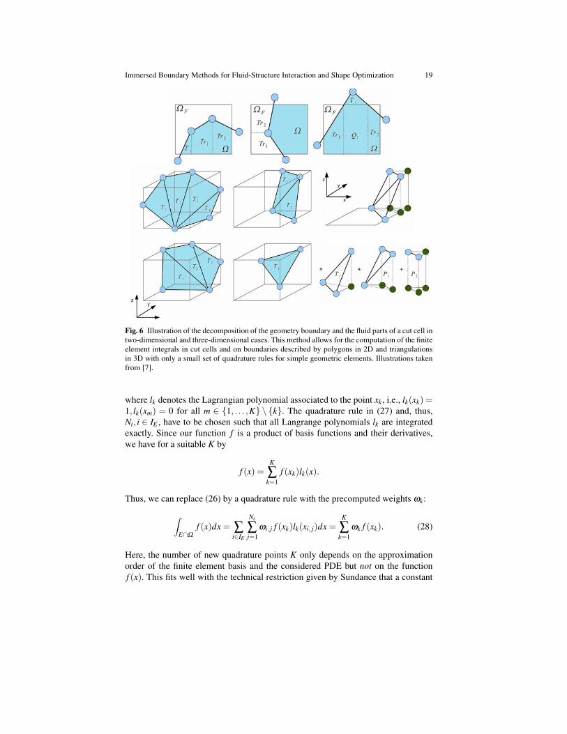
To implement Nitsche’s method for flow equations on complex and moving do-mains, we first need some technical ingredients, i.e., volume integrals over cut cellsintegrating only over the part of a grid element that is inside the fluid domain andboundary integrals over the domain boundary. Both require an explicit represen-tation of the domain boundary. As we work with second-order discretizations, wecan use simple polygons (in 2D)3 or surface triangulations (in 3D). Figure 6 illus-trates the representation of domains and cut cell volumes. In 2D, we allow a cell tobe intersected by an arbitrary polygon. In this case, we can always find a suitabledecomposition of the remaining fluid part of a cell into simple trapezoidals and tri-angles. In 3D, the analogue process with arbitrary surface triangulations intersectinga cubic grid element would lead to a too large amount of different cases and, thus,is not feasible. Therefore, we restrict to cases, where all cell edges are intersectedat most once by the surface triangulation. Connecting these intersection points bystraight lines leads to a new, approximate, but still second-order accurate surfacetriangulation and only a small number of cases as displayed in Fig. 6. In both cases,2D and 3D, we end up with a decomposition of the fluid part of the cut cell into sim-ple elements Ei, i ∈ IE of given type that can be integrated up to machine precisionwith suitable quadrature rules. The same holds for the surface integrals.

For the volume integrals over cut cells, we thus have

∫E∩Ω

f (x)dx = ∑i∈IE

∫Ei

f (x)dx = ∑i∈IE

Ni

∑j=1

ωi, j f (xi, j)dx, (26)

where Ei, i ∈ IE , are the simple subcells into which we decompose of the fluid partof the cell and xi, j, j = 1, . . . ,Ni, are the quadrature points used in subcell i. With thisformula, we can compute all cut cell integrals up to machine precision. However,this method can lead to a large number of quadrature points xi, j in particular in 3Dand for higher order basis functions. Therefore, we reduce the number of quadraturepoints by using precomputed weights

ωk = ∑i∈IE

Ni

∑j=1

ωi, jlk(xi, j),k = 1, . . . ,K (27)

3 For 2D geometries, there is also an implementation in Sundance that can deal with analyticalgeometry representations (such as a circle) that are then automatically approximated by a suitablepolygon internally [7].


Fig. 6 Illustration of the decomposition of the geometry boundary and the fluid parts of a cut cell intwo-dimensional and three-dimensional cases. This method allows for the computation of the finiteelement integrals in cut cells and on boundaries described by polygons in 2D and triangulationsin 3D with only a small set of quadrature rules for simple geometric elements. Illustrations takenfrom [7].

where lk denotes the Lagrangian polynomial associated to the point xk, i.e., lk(xk) =1, lk(xm) = 0 for all m ∈ 1, . . . ,K \ k. The quadrature rule in (27) and, thus,Ni, i ∈ IE , have to be chosen such that all Langrange polynomials lk are integratedexactly. Since our function f is a product of basis functions and their derivatives,we have for a suitable K by

f (x) =K

∑k=1

f (xk)lk(x).

Thus, we can replace (26) by a quadrature rule with the precomputed weights ωk:

∫E∩Ω

f (x)dx = ∑i∈IE

Ni

∑j=1

ωi, j f (xk)lk(xi, j)dx =K

∑k=1

ωk f (xk). (28)

Here, the number of new quadrature points K only depends on the approximationorder of the finite element basis and the considered PDE but not on the functionf (x). This fits well with the technical restriction given by Sundance that a constant


number of quadrature points is to be used throughout the whole computational grid.Whenever the domain Ω changes, the weights ωk have to be recomputed in a loopover all cut cells computing the local quadrature points xi, j for each subcell on thefly.

Line or surface boundary integrals are computed analogously. However, we donot use precomputed weights here as 1) some boundary integrals involve normalvectors that are different for each subpart of the boundary inside a given cell, 2)boundary integrals are cheaper such that we can afford storing all quadrature points,3) three-dimensional cases require the usage of data points in the vicinity but not di-rectly on the boundary due to the approximation of the original triangulation withineach cut cell.

Technically, the implementation of Nitsche’s method in Sundance requires newuser interfaces for

• description of the geometry by a polygon/triangulation• cell filters selecting intersected cells,• integrals over cut cells, and• boundary integrals.

To realize moving boundaries in Sundance, several data have to be updated afterchanging of the geometry:

• the positions of the surface polygon or triangulation,• internal information such as IDs of cells cut by components of the surface object,• precomputed quadrature weights for the finite element integration during matrix

assembly,• entries of the system matrix/matrices.

To move surface nodes, we use the local surface velocity (given by the bound-ary conditions) at the respective position. The update of all internal geometryinformation is hidden from the user in the function .update(). The function.reAssembleProblem() recomputes quadrature weights and assembles thenew system matrix/matrices.

8 Fluid-Structure Simulations Using Nitsche’s Method

The suitability and accuracy of our method using Cartesian grids in combinationwith Nitsche’s method for simple model problems and pure flow simulation in staticand moving domains has been shown in [7, 8]. In this paper, we focus on resultsobtained for a multiphysics application class, i.e., fluid-structure interactions.

Our Partitioned Approach for Coupled Fluid-Structure Simulation in Sun-dance. We use the incompressible Navier-Stokes equations (1) and (2) and combinethem with the structural equation (3) and the coupling conditions (4) and (5) to afull fluid-structure simulation environment.


As we use an Eulerian fixed grid approach as described in the previous sectionsfor the fluid part, but the common Lagrangian approach with a classical enforce-ment of boundary conditions for the structure part, we have to couple the interfacedisplacements in addition:

ΓF = x+us|x ∈ ΓL, (29)

where ΓF is the internal moving geometry description (polygon or surface triangula-tion) of the fluid solver and ΓL the Lagrangian structure surface description (constantthroughout the simulation). See Fig. 7 for an illustration. Technically, this is real-ized in Sundance using twin polygons or twin triangulations. The nodes of these twopolygons or triangulations are connected via a bijective mapping from the node setof the first polygon/triangulation to the node set of the second polygon/triangulationas illustrated in Fig. 7 by the dashed lines. Whenever a value of an unknown functionis changed on a node of one polygon/triangulation, it is automatically also changedon the respective node of the twin polygon/triangulation.

Fig. 7 Left: Eulerian (fluid) and Lagrangian (structure) view of a simple two-dimensional movingstructure. The green circles mark the nodes of the polygonal geometry description in the fluidsolver, whereas the light grey circles are the boundary vertices of the Lagrangian reference domainon the structure side. Right: Schematic view of the staggered coupling approach for partitionedfluid-structure interaction simulations. After executing a time step of the flow solver, forces at(29) are transfered to the structure solver, which subsequently executes its time step and producesdisplacements and velocities at the wet surface as an output, which serve as a boundary conditionat (29) for the next fluid step and so forth. This process is repeated until the residual of the fix-pointequation for the displacements falls below a given threshold. Illustrations taken from [7].

As a time discretization, we use implicit Euler for the fluid and structure equa-tions. To perform a time step of the whole coupled problem, the partitioned ap-proach requires an iterative execution of fluid and structure solver steps involvingan exchange of boundary values. We use the widespread staggered coupling ap-proach as shown in Fig. 7. For incompressible fluids, this coupling in general leadsto unstable time stepping if used in an explicit manner (only one fluid and structurestep per time step). Thus, we have to iteratively repeat the fluid and structure stepsuntil the residual of the associated fixed point equation for the displacements at thewet surface falls below a certain threshold. To achieve convergence of the fluid-structure iterations, we use Aitken underrelaxation when transferring displacementsfrom the structure solver to the flow solver. Aitken underrelaxation determines an


adaptive scalar underrelaxation factor in each iteration [24]. More sophisticated cou-pling methods such as interface quasi-Newton schemes [14] or multilevel [46, 9]approaches yield an even faster convergence. However, for our purpose of showingthe potential of Nitsche’s method for the simulation of fluid-structure interaction onstructured Cartesian grids, Aitken underrelaxation suffices.

In the following, we present some of our numerical results for fluid-structureinteraction scenarios in 2D and 3D. Further results can be found in [7].

Rigid Body Motion in 3D. Our first scenario is the three-dimensional rigid bodymotion of a spherical object in a flow channel as shown in Fig. 8. In a channel ofdimensionless size 8×4×4, a sphere with dimensionless radius one and a dimen-sionless mass of one moves according to Newton’s law of motion and the sum offorces exerted on it by the fluid flow. The fluid has the dimensionless density oneand the inflow speed is set to 2.25. We keep the sphere fixed until dimensionlesstime T = 0.2. After that initial period, the sphere is released and accelerated by thesurrounding fluid flow. The fluid flow is simulated on a very coarse regular Cartesianmesh with only 13× 9× 9 elements, whereas the sphere’s surface is approximatedby 500 triangles with 252 nodes. Due to the relatively large structure density and therather small radius of the sphere, this example allowed for explicit coupling, i.e., weperformed only one fluid and structure step in each time step. Figure 8 shows thegood solution quality in spite of the very coarse fluid mesh resolution. The sphereexhibits a smooth movement in flow direction as expected for a correct solution. Theforces in x-direction show some unphysical peaks due to the time integration issuesfor moving geometries mentioned above. Depending on the the state of the simula-tion, these peaks can even result in negative forces slowing down the motion of thesphere in x-direction. However, each of these peaks decays very fast and, thus, doesnot influence the overall solution significantly. The height of the peaks obviouslydepends on the time step size and the spatial resolution.

Fig. 8 Simulation of a rigid body motion of a sphere in a fluid flow using a very coarse Cartesianmesh. Left: absolute velocities in a plane of the fluid domain; middle: force vectors acting on thesphere; right: total forces in flow direction acting on the sphere plotted over time. The forces decayto zero as the sphere accelerates. Illustrations taken from [7].

Two-Dimensional Benchmarks. To verify our implementation by more reli-able data than heuristic observations as in the 3D example above, we simulated


2D benchmark scenarios for fluid-structure interaction proposed in [22, 23]. Thescenario consists of a channel flow with an embedded spherical obstacle and anattached flexible bar structure. The spherical obstacle itself remains fixed, but thebar bends in a steady state (FSI1) or oscillating (FSI3) manner depending on theReynolds number of the channel flow. Due to a slight offset in vertical direction,the structure is exposed to both horizontal and vertical forces. Figure 9 shows thegeometric setup of the benchmark. The structure is a super-elastic compressiblematerial with ρs = 103 kg

m3 and Young’s modulus E = 1.4 ·106 kgm3 . We discretize the

Navier-Stokes equations using Q2Q1 and the structure using Q1 elements. For thisscenario, an implicit coupling with several fluid-structure iterations is mandatory toachieve stable results. We use ε = 10−6 as a stopping criterion for our staggeredfluid-structure iterations with a constant underrelaxation factor ω = 0.3.

Fig. 9 Two-dimensional fluid-structure interaction benchmark scenario from [22, 23]. The sce-nario shows a fixed and rigid spherical object with an attached super-elastic compressible flapstructure embedded in a channel flow. Left: Scenario geometry with a slight offset of the structurefrom the channel axis. Right: domain decomposition of the structure and the fluid part for a parallelsimulation with four processors. Illustrations taken from [7].

The FSI1 scenario is a stationary case with a steady state flow and a slight con-stant bending of the elastic bar structure in y-direction. The inflow velocity is set tov f = 0.2 m

s . Convergence within a time step was achieved after 20 iterations on av-erage. Table 3 shows the computed values for the displacements of the tip of the barin x- and y-direction as well as the total drag and lift forces exerted on the structureby the fluid. The total forces have been calculated by curve integrals on the poly-gon. The table shows already a good agreement with the benchmark values for thecoarsest mesh resolution and a convergence towards the correct values with increas-ing resolution. The simulations for this scenario have been performed in parallelusing four processors for each, fluid and structure solver, and two processors for thesurface polygon. The associated domain decomposition of the fluid and structuredomain is shown in Fig. 9. As a solver, we used the SuperLU-DIST linear solverwithin an outer non-linear NOX solver4. This combination resulted in an acceptablebut not yet optimal parallel efficiency of 54% [7]. Note that the simple load balanc-ing strategy, a quasi-serial phase for the surface polygon, and further optimizationpotential in the storage of grid partitiones currently limits the scalability, a fact thatshall be improved in further development steps.

4 trilinos.sandia.gov/packages/nox/


cells f luid cellsstruct linespoly displ. x displ. y drag lift2,610 3,380 136 1.86 ·10−5(18%) 1.230 ·10−3(50%) 14.078(1.5%) 0.8202(7.4%)

36,666 13,370 1,093 2.21 ·10−5(2.6%) 0.703 ·10−3(14%) 14.198(0.7%) 0.8101(6.1%)

54,104 13,370 1,093 2.18 ·10−5(3.5%) 0.846 ·10−3(5.2%) 14.224(0.5%) 0.7930(3.8%)

ref. values 2.27 ·10−5 0.821 ·10−3 14.295 0.7638

Table 3 Simulation results for two different mesh resolutions and the benchmark scenario FSI3from [22, 23]. The displacement of the tip of the bar in x- and y-direction, the total drag, and thetotal lift force are compared with the benchmark reference values in [23]. Numbers in parenthesesdenote the absolute value of the relative error.

The FSI3 is a transient case with a higher inflow velocity of 2 ms that leads to

an oscillatory movement of the flexible bar and also requires a strong, i.e., implicitcoupling of fluid and structure. We used Aitken underrelaxation resulting in 11 iter-ations per time step on average. Figure 10 and Tab. 4 show the resulting movementof the bar and the respective tip displacements, total drag, and total lift with theirmean value, the amplitude of their oscillation, and their frequency. The comparisonwith the benchmark reference values from [23] shows a good agreement. However,for more reliable convergence statements, additional mesh resolutions have to beexamined in addition in future work.

Fig. 10 Simulation results for the transient FSI3 benchmark from [22, 23]. Left: two snapshots ofthe solution with colours representing the absolute fluid velocities and the structural displacement.Arrows show the forces acting on the structure; middle: time variant total drag; right: time varianttotal lift. Plots taken from [7].


cells f luid cellsstruct linespoly displ. x displ. y drag lift

2,507 864 136−0.02866

±0.02857[11.1]−0.00111±0.03301[5.5]

524.5±23.5[11.1]

56.50±214.50[5.5]

5,133 864 136−0.00288

±0.00282[11.4]0.00166

±0.03452[5.7]532

±25[11.4]−1.5

±229.50[5.7]

ref. values−0.00269

±0.00253[10.9]0.00148

±0.03438[5.3]457.3

±22.66[10.9]2.2

±149.78[5.3]

Table 4 Simulation results for two different mesh resolutions and the benchmark scenario FSI3from [22, 23]. For all measured values, i.e., displacement of the tip of the bar in x- and y-direction,total drag, and total lift force, offset, amplitude, and frequency (in [·]) are measured and comparedwith the benchmark reference values in [23].

Three-Dimensional Bending Tower. As a three-dimensional example for thecoupled simulation of fluid-structure interactions with a moving flexible structure,we consider a channel flow with a bending tower (see Fig. 11). The fluid has aagain density of 103 kg

m3 and a parabolic inflow profile with maximal velocity 0.45 ms .

The bending tower is modeled by a super-elastic material with Young’s modulusE = 0.4 ·106 kg

ms2 . The tower has a size of 0.05m×0.25m×0.1m. We use an adaptiveCartesian grid for the flow solver with adaptive refinement in a rectangular domainaround the tower. The resolution of the coarse background mesh is 27×7×7 cells.We discretized the Navier-Stokes equations with stabilized Q1Q1 and the structureequation with Q1 elements. The stabilized Q1Q1 are known to work well in three-dimensional fluid benchmarks, e.g., in [40]. The coupling iterations are performedwith an underrelaxation factor ω = 0.3 up to an error tolerance ε = 10−6. Figure 11shows the resulting bending of the tower, which can not be verified by benchmarkvalues but gives reasonable results [7].

9 Shape Optimization with the Immersed Boundary Approach

We now demonstrate the application of our immersed boundary approach to shapeoptimization problems. To this end, we consider the Stokes equations

−ν∆v+∇p = 0, divv = 0, v|∂Ω\Γ = d, v|Γ = 0. (30)

Here, Ω =ΩC \B, where ΩC is a rectangular channel and B is a body with boundaryΓ . The goal is to find a design for B such that the cost functional

J(v,Ω) = ν

∫Ω

‖∇v‖2 dx, (31)

which is related to the drag of the body, is minimized. Here, B shall have a prescribedvolume and (except possibly at the front and rear tip points) a sufficiently smoothboundary. The latter condition is required to ensure existence of optimal shapes.


Fig. 11 Three-dimensional simulation of a bending tower in a channel flow. The upper pictureshows the tower and the surrounding computational grid with an adaptive refinement in a blockaround the tower. Left: flow field and fluid pressure; right: bending of the tower. Illustrations takenfrom [7].

Denoting by (v(Ω), p(Ω)) the solution of the Stokes equations on the domainΩ , the shape derivative of j(Ω) := J(v(Ω),Ω) can be shown to satisfy

d j(Ω)[V ] =−ν

∫Γ

‖∂nv(Ω)‖2 V ·ndS(x), (32)

see [32, pp. 29/30]. A similar result holds for the more general case of the Navier-Stokes equations, but it then involves the adjoint state [32, pp. 31/32]. The Stokesequations in combination with the cost function (31) allow to express all occurrencesof the adjoint state in terms of v, thus making the adjoint state superfluous.

The shape of the body B is described by a closed polygon with nodes (x0,y0),. . ., (x2m−1,y2m−1). Here, the next point (x2m,y2m) would correspond to (x0,y0).We only consider shapes that are symmetric with respect to a horizontal center line(parallel to the x-axis):

y0 = ym, xi = x2m−i, y0− yi = y2m−i− y0 (1≤ i < m).

We do not work directly with this representation, but use polar coordinates with re-spect to (a,b) = ((x0+xm)/2,y0). For i = 0, . . . ,m, the i-th point is allowed to move


along the radial ray (a,b)+R(xi−a,yi−b). The transformed point is parameterizedby the radial scaling ri: (xi(ri),yi(ri)) = (a,b)+ ri(xi− a,yi− b). Due to our sym-metry assumptions, specifying r = (r0, . . . ,rm)

T uniquely characterizes the shape ofthe polygonal boundary of the deformed body.

In the function space setting, the existence of optimal shapes requires coercivityof the cost function in a sufficiently strong shape space. In the discrete setting, weenforce some amount of smoothness by adding an H1-like regularization for r to thecost function (31). Also, we work with an H1-like inner product by switching to theparameterization z∈Rm+1 with ri =∑

ij=0 z j. We then have z0 = r0 and zi = ri−ri−1,

i > 0. In our computations, we work with the body B(z) parameterized by z. We thencan use an l2-norm for the regularization:

γmm

∑i=1

z2i . (33)

The factor m stems from the fact that if we view the ri as evaluations of a functionr(τ) on an equidistant grid τ0, . . . ,τm with τi = iδ , δ = 1/m, then mzi = (ri−ri−1)/δ

approximates r′(τi−δ/2). Hence,∫ 1

0r′(τ)2 dτ ≈ δ

m

∑i=1

r′(τi−δ/2)2 ≈ mm

∑i=1

z2i . (34)

For evaluating the discrete version jh(z) of the cost function (31) and its gradient∇ jh(z) at a point z in parameter space, we solve the Stokes equation, discretized byNitsche’s method, on Ω(z) = ΩC \B(z) to obtain the discrete velocity field vh. Then

J(vh,Ω(z)) = ν

∫Ω(z)‖∇vh‖2 dx (35)

is computed and the regularization (33) is added. For evaluating the gradient ∇ jh(z)at a point z we use that the map z 7→ (xi(z),yi(z))−(a,b) is linear. Thus, the directionof variation ei = (δik)0≤k≤m of z is linearly mapped to the direction of variation(xp(ei),yp(ei))− (a,b) of the p-th polygon node (xp(z),yp(z)).

Therefore, for the z-variation direction ei, the value of the corresponding dis-placement field direction V = V p at the polygon’s pth node is (xp(ei),yp(ei))−(a,b). To compute ∇zi jh(z) we thus evaluate

−ν

∫Γ (z)‖∂nvh‖2 V p ·ndS(x). (36)

The required methods, in particular the conversion of nodal values along the polygoninto expressions that can appear in line integrands over the polygon curve have allbeen implemented by us for general use in Sundance.

We stress that the formula (36) for ∇zi jh(z) is not fully exact since (32) requiresthe exact solution v of the PDE, whereas vh is only a numerical approximation that,


in addition, depends not only on the shape of Ω(z) but also on the underlying FEMmesh.

In the numerical test presented here we require also symmetry with respect to thevertical center line passing through (a,b). To this end, we choose m = 2l and onlyprescribe the lower left quarter of the profile, which is described by z0, . . . ,zl , wherewe require xl = a. Thus, (x0,y0) lies on the horizontal center line and (xl ,yl) lieson the vertical center line. The rest of the profile is obtained by symmetry and thecenter of mass is then automatically fixed to (a,b).

We impose a constant volume constraint vol(Ω(z)) = cvol, with cvol denoting thevolume of the initial shape. The volume and its derivative can be obtained conve-niently by, e.g., the Leibniz sector formula. We also pose inequality constraints onthe maximum radial elongation / contraction: 1/2 ≤ ri(z) ≤ 2 for all i. The boundsare chosen such that the constraints do not become active, but they can help avoidingtoo strong initial design changes during optimization.

We choose ΩC = (0,2.5)× (0,1), (a,b) = (0.75,0.5), the tip point of the initialshape is at (0.67,0.5) and the initial volume is 0.0163672. We impose Dirichletconditions v = (0.2,0) on the boundary of ΩC and v = 0 on ∂B(z). The boundaryconditions on ∂B(z) are enforced by Nitsche’s method. Figure 12 shows the initialshape on the left. The boundary of the body is described by 2m = 4l = 80 points,i.e., we have m = 40, l = 20. We use a Taylor-Hood discretization (biquadratic forthe velocity, bilinear for the pressure) on a Cartesian mesh with hanging nodes.The grid consists of a 145×101 mesh, where the 23×41 subgrid centered around(a,b) = (0.75,0.5) is refined by cellwise trisection in both space dimensions to aobtain a 69×123 grid on this subregion. The regularization parameter is γ = 0.006.

We implemented a general purpose C++ interface that couples our Sundancesimulation, which solves the Stokes equation and evaluates jh, ∇ jh, etc., to the in-terior point optimization software IPOPT [44]. We use the limited memory BFGSapproximation of the Lagrange function’s Hessian matrix that is built into IPOPT.

As mentioned, due to the fact that the shape derivative formula is only exactin the continuous setting, the computed derivatives are not exact derivatives of thediscretized cost function. Thus, we can achieve only a moderate (but sufficient)accuracy in satisfying the stopping criteria of the NLP solver IPOPT.

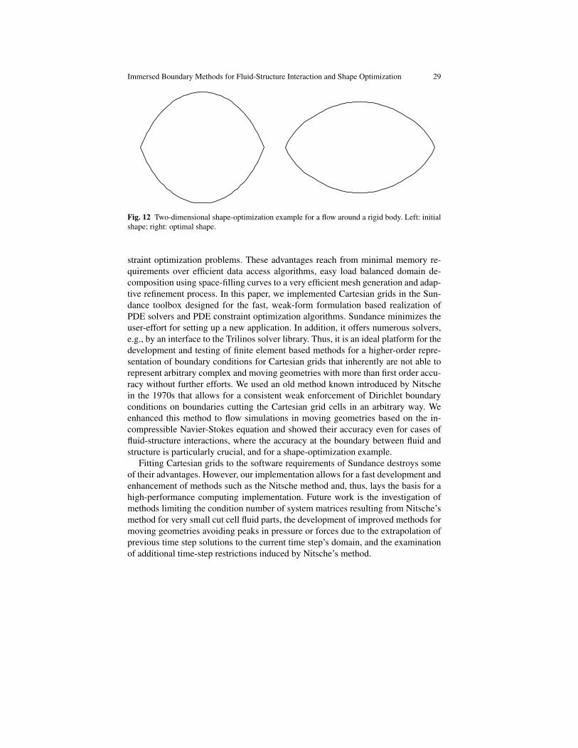
Starting with the initial shape shown on the left in Fig. 12, we obtain a solution(with the achievable accuracy due to inexact discrete shape gradient) after 10 IPOPTiterations. The objective function is reduced by 6.9 %. The optimal shape is shownon the right in Fig. 12. Note that the result depends on the chosen regularization.

10 Conclusion

We proposed an implementation of adaptive Cartesian grids in combination withNitsche’s method for an accurate enforcement of boundary conditions on complexand moving domains. Adaptive Cartesian meshes have severe advantages for anefficient implementation of solvers for partial differential equations and PDE con-


Fig. 12 Two-dimensional shape-optimization example for a flow around a rigid body. Left: initialshape; right: optimal shape.

straint optimization problems. These advantages reach from minimal memory re-quirements over efficient data access algorithms, easy load balanced domain de-composition using space-filling curves to a very efficient mesh generation and adap-tive refinement process. In this paper, we implemented Cartesian grids in the Sun-dance toolbox designed for the fast, weak-form formulation based realization ofPDE solvers and PDE constraint optimization algorithms. Sundance minimizes theuser-effort for setting up a new application. In addition, it offers numerous solvers,e.g., by an interface to the Trilinos solver library. Thus, it is an ideal platform for thedevelopment and testing of finite element based methods for a higher-order repre-sentation of boundary conditions for Cartesian grids that inherently are not able torepresent arbitrary complex and moving geometries with more than first order accu-racy without further efforts. We used an old method known introduced by Nitschein the 1970s that allows for a consistent weak enforcement of Dirichlet boundaryconditions on boundaries cutting the Cartesian grid cells in an arbitrary way. Weenhanced this method to flow simulations in moving geometries based on the in-compressible Navier-Stokes equation and showed their accuracy even for cases offluid-structure interactions, where the accuracy at the boundary between fluid andstructure is particularly crucial, and for a shape-optimization example.

Fitting Cartesian grids to the software requirements of Sundance destroys someof their advantages. However, our implementation allows for a fast development andenhancement of methods such as the Nitsche method and, thus, lays the basis for ahigh-performance computing implementation. Future work is the investigation ofmethods limiting the condition number of system matrices resulting from Nitsche’smethod for very small cut cell fluid parts, the development of improved methods formoving geometries avoiding peaks in pressure or forces due to the extrapolation ofprevious time step solutions to the current time step’s domain, and the examinationof additional time-step restrictions induced by Nitsche’s method.


References

1. I. Babuska. Numerical Solution of Boundary Value Problems by the Perturbed VariationalPrincile. Technical Note BN-624, 1969.

2. I. Babuska. The finite element method with penalty. Mathematics of Computation, 27:122–128, 1973.

3. Y. Bazilevs, C. Michler, V. M. Calo, and T. J. R. Hughes. Isogeometric variational multiscalemodeling of wall-bounded turbulent flows with weakly enforced boundary conditions on un-stretched meshes. Computer Methods in Applied Mechanics and Engineering, 199:780–790,2010.

4. R. Becker. Mesh Adaption for Dirichlet Flow Control via Nitsche’s Method. Communicationin Numerical Methods in Engineering, 18:669–680, 2002.

5. M. Behr. Simplex space-time meshes in finite element simulations. Int. J. Numer. Meth.Fluids, 57:1421–1434, 2008.

6. J. A. Bello, E. Fernandez-Cara, J. Lemoine, and J. Simon. The differentiability of the dragwith respect to the variations of a Lipschitz domain in a Navier-Stokes flow. SIAM J. ControlOptim., 35(2):626–640, 1997.

7. J. Benk. Immersed Boundary Methods within a PDE Toolbox on Distributed Memory Systems.PhD thesis, Technische Universitat Munchen, 2012.

8. J. Benk, M. Mehl, and M. Ulbrich. Sundance PDE solvers on Cartesian fixed grids in complexand variable geometries. In Proceedings of the ECCOMAS Thematic Conference CFD &Optimization, Antlya, Turkey, May 23-25, 2011, May 2011.

9. H. Bijl, A. H. van Zuijlen, and S. Bosscher. Two level algorithms for partitioned fluid-structureinteraction computations. In P. Wesseling, E. Onate, and J. Periaux, editors, ECCOMAS CFD2006, European Conference on Computational Fluid Dynamics. TU Delft, 2006.

10. A. N. Bugrov and S. Smagulov. Fictitious Domain Method for Navier-Stokes Equations.Mathematical model of fluid flow, Novosibirsk, pages 79–90, 1978.

11. H.-J. Bungartz, B. Gatzhammer, M. Mehl, and T. Neckel. Partitioned simulation of fluid-structure interaction on Cartesian grids. In H.-J. Bungartz, M. Mehl, and M. Schafer, edi-tors, Fluid-Structure Interaction – Modelling, Simulation, Optimisation, Part II, volume 73 ofLNCSE, pages 255–284. Springer, Berlin, Heidelberg, 2010.

12. H.-J. Bungartz, M. Mehl, and T. Weinzierl. A parallel adaptive Cartesian PDE solver usingspace–filling curves. In E.W. Nagel, V.W. Walter, and W. Lehner, editors, Euro-Par 2006,Parallel Processing, 12th International Euro-Par Conference, volume 4128 of Lecture Notesin Computer Science, pages 1064–1074, Berlin Heidelberg, 2006. Springer-Verlag.

13. C. Bursteddea, L.C. Wilcox, and O. Ghattas. p4est: Scalable algorithms for parallel adaptivemesh refinement on forests of octrees. SIAM Journal on Scientic Computing, 33(3):1103–1133, 2011.

14. J. Degroote, K.J. Bathe, and J. Vierendeels. Performance of a new partitioned procedure versusa monolithic procedure in fluid-structure interaction. Comput. Struct., 87:793–801, 2009.

15. R. Glowinski, T.W. Pan, T.I. Hesla, D.D. Joseph, and J.Periaux. A Fictitious Domain Approachto the Direct Numerical Simulation of Incompressible Viscous Flow past Moving Rigid Bod-ies: Application to Particulate Flow. Journal of Computational Physics, 169:363–426, 2001.

16. M. Griebel, Th. Dornseifer, and T. Neunhoeffer. Numerical Simulation in Fluid Dynamics, aPractical Introduction. SIAM, 1998.

17. M. Griebel and G. Zumbusch. Hash based adaptive parallel multilevel methods with space-filling curves. In H. Rollnik and D. Wolf, editors, NIC Symposium 2001, volume 9 of NICSeries, ISBN 3-00-009055-X, pages 479–492, Germany, 2002. Forschungszentrum Julich.

18. Ph. Guillaume and M. Masmoudi. Computation of high order derivatives in optimal shapedesign. Numer. Math., 67(2):231–250, 1994.

19. F. H. Harlow and J. E. Welch. Numerical calculation of time-dependent viscous incompress-ible flow of fluid with a free surface. Physics of Fluids, pages 2182–2189, 1965.


20. M. Heroux, R. Bartlett, V. Howle, R. Hoekstra, J. Hu, T. Kolda, R. Lehoucq,K. Long, R. Pawlowski, E. Phipps, A. Salinger, H. Thornquist, R. Tuminaro, J. Wil-lenbring, and A. Williams. An Overview of Trilinos. SAND REPORT, 2003.http://trilinos.sandia.gov/TrilinosOverview.pdf.

21. M. Hinze, R. Pinnau, M. Ulbrich, and S. Ulbrich. Optimization with PDE constraints, vol-ume 23 of Mathematical Modelling: Theory and Applications. Springer, New York, 2009.

22. J. Hron and S. Turek. Proposal for numerical benchmarking of fluid-structure interactionbetween elastic object and laminar incompressible flow. In H.-J. Bungartz and M. Schafer,editors, Fluid-Structure Interaction, number 53 in Lecture Notes in Computational Scienceand Engineering, pages 371–385. Springer-Verlag, 2006.

23. J. Hron and S. Turek. Numerical benchmarking of fluid-structure interaction between elasticobjects and laminar incompressible flow. In H.-J. Bungartz, M. Mehl, and M. Schafer, edi-tors, Fluid-Structure Interaction – Modelling, Simulation, Optimisation, Part II, volume 73 ofLNCSE. Springer, Berlin, Heidelberg, 2010.

24. U. Kuettler and W.A. Wall. Fixed-point fluid-structure interaction solvers with dynamic re-laxation. Computational Mechanics, 43(1):61–72, 2008.

25. V.R. Yarberry L.A. Schoof. Exodus II: A Finite Element Data Model. Sandia Report,SAND92-2137, 1994.

26. R.J. LeVeque. Cartesian grid methods for flow in irregular regions. In K.W. Morton and M.J.Baines, editors, Num. Meth. Fl. Dyn. III, pages 375–382. Clarendon Press, 1988.

27. K. Long. Sundance 2.0 Tutorial, 2004. http://prod.sandia.gov/techlib/access-control.cgi/2004/044793.pdf.

28. K. R. Long, R. C. Kirby, and B. van Bloemen Waanders. Unified embedded parallel finite ele-ment computations via software-based Frechet differentiation. SIAM J. Scientific Computing,32(6):3323–3351, 2010.

29. MathWorks. MATLAB The Language of Technical Computing.http://www.mathworks.com/products/matlab/index.html; last visted: September 2012.

30. R. Mittal and G. Iaccarino. Immersed boundary methods. Annu. Rev. Fluid Mech., 37:239–261, 2005.

31. N. Moes, J. Dolbow, and T. Belytschko. A finite element method for crack growth withoutremeshing. International Journal for Numerical Methods in Engineering, 46:131150, 1999.

32. B. Mohammadi and O. Pironneau. Applied Shape Optimization for Fluids. Oxford UniversityPress, 2001.

33. F. Murat and J. Simon. Etudes de probl`mes d’optimal design. Lecture Notes in ComputerScience, 41:54–62, 1976.

34. J. Nitsche. Uber ein Variationsprinzip zur Losung von Dirichlet-Problemen bei Verwendungvon Teilraumen, die keinen Randbedingungen unterworfen sind. Abhandlungen aus demMathematischen Seminar der Universitat Hamburg, 36:9–15, 1971. 10.1007/BF02995904.

35. W. F. Noh and P. Woodward. SLIC (Simple Line Interface Calculation). In A. I. van de Voorenand P. J. Zandbergen, editors, Proceedings of 5th International Conference of Fluid Dynamics,Lecture Notes in Physics, pages 330–340. 1976.

36. S. Osher and J. A. Sethian. Fronts propagating with curvature-dependent speed: Algorithmsbased on Hamilton-Jacobi formulations. J. Comput. Phys., pages 12–49, 1988.

37. C. S. Peskin. Numerical analysis of blood flow in the heart. J. Comput. Phys., pages 220–252,1977.

38. J.E. Pilliod and E.G. Puckett. Second-order accurate volume-of-fluid algorithms for trackingmaterial interfaces. Journal of Computational Physics, pages 465–502, 2004.

39. E. Rank, S. Kollmannsberger, Ch. Sorger, and A. Duster. Shell finite cell method: A highorder fictitious domain approach for thin-walled structures. Computer Methods in AppliedMechanics and Engineering, 200(45/46):3200 – 3209, 2011.

40. M. Schafer and S. Turek. Benchmark computations of laminar flow around a cylinder. InFlow simulation with high-performance computers 2, volume 52 of Notes on numerical fluidmechanics, pages 547–566. Vieweg, 1996.


41. W.J. Schroeder, K.M. Martin, and W.E. Lorensen. The Design and Implementation of anObject-Oriented Toolkit For 3D Graphics And Visualization. In Proceedings of the 7th Con-ference on Visualization ’96, VIS ’96, pages 93–ff. IEEE Computer Society Press, 1996.

42. J. Sokolowski and J.-P. Zolesio. Introduction to Shape Optimization: Shape sensitivity analy-sis. Springer, Berlin, 1992.

43. T. E. Tezduyar, M. Behr, S. Mittal, and A.A. Johnson. Computation of unsteady incom-pressible flows with the stabilized finite element methods: space-time formulations, iterativestrategies and massively parallel implementations. Asme Pressure Vessels Piping Div PublPVP, 246:7–24, 1992.

44. A. Wachter and L. T. Biegler. On the implementation of an interior-point filter line-searchalgorithm for large-scale nonlinear programming. Mathematical Programming, pages 25–57,2006.

45. T. Weinzierl and M. Mehl. Peano – a traversal and storage scheme for octree-like adaptivecartesian multiscale grids. SIAM Journal on Scientific Computing, 33(5):2732–2760, 2011.

46. S. Yigit, M. Heck, D. C. Sternel, and M. Schafer. Efficiency of fluid-structure interactionsimulations with adaptive underrelaxation and multigrid acceleration. Int. J. Multiphysics,1:85–99, 2007.

47. J.-P. Zolesio and M.C. Delfour. Shapes and Geometries: Analysis, Differential Calculus andOptimization. SIAM, 2001.

Date post:	10-Jul-2020
Category:	Documents
Upload:	others
View:	8 times
Download:	0 times

Immersed Boundary Methods for Fluid-Structure Interaction ...€¦ · Optimization within an...

Documents