HAL Id: hal-01605797 https://hal.archives-ouvertes.fr/hal-01605797 Submitted on 5 Jun 2020 HAL is a multi-disciplinary open access archive for the deposit and dissemination of sci- entific research documents, whether they are pub- lished or not. The documents may come from teaching and research institutions in France or abroad, or from public or private research centers. L’archive ouverte pluridisciplinaire HAL, est destinée au dépôt et à la diffusion de documents scientifiques de niveau recherche, publiés ou non, émanant des établissements d’enseignement et de recherche français ou étrangers, des laboratoires publics ou privés. Distributed under a Creative Commons Attribution - NonCommercial - NoDerivatives| 4.0 International License Impact of agricultural landscape on honey reserves in bee colonies Domitille Pouliquen To cite this version: Domitille Pouliquen. Impact of agricultural landscape on honey reserves in bee colonies. 2016, 58 p. hal-01605797
Transcript
HAL Id: hal-01605797https://hal.archives-ouvertes.fr/hal-01605797
Submitted on 5 Jun 2020
HAL is a multi-disciplinary open accessarchive for the deposit and dissemination of sci-entific research documents, whether they are pub-lished or not. The documents may come fromteaching and research institutions in France orabroad, or from public or private research centers.
L’archive ouverte pluridisciplinaire HAL, estdestinée au dépôt et à la diffusion de documentsscientifiques de niveau recherche, publiés ou non,émanant des établissements d’enseignement et derecherche français ou étrangers, des laboratoirespublics ou privés.
Distributed under a Creative Commons Attribution - NonCommercial - NoDerivatives| 4.0International License
Impact of agricultural landscape on honey reserves inbee colonies
Domitille Pouliquen
To cite this version:Domitille Pouliquen. Impact of agricultural landscape on honey reserves in bee colonies. 2016, 58 p.�hal-01605797�
Signalement du mémoire : Impact du paysage agricole sur les réserves de miel des colonies d’abeilles, 51 pages,4 tableaux, 36 graphiques, 60 sources bibliographies, 8 annexes.
Mots clés : Abeille domestique, paysage, potentiel mellifère, réserves de miel. RESUME D’AUTEUR
Dans des systèmes agricoles intensifs la pollinisation des cultures et des plantes sauvages est menacée par le fort déclin des pollinisateurs. Le déclin de l’abeille domestique semble être le résultat de plusieurs stress environnementaux tel que les maladies, les pesticides et la diminution des ressources florales. L’évaluation de la production de nectar des différentes espèces présentes est nécessaire pour pouvoir concentrer les efforts de protection et de conservations sur les espèces clés pour les abeilles. L’objectif de cette étude est d’évaluer la contribution saisonnière des plantes oléagineuses ayant une floraison massive (colza et tournesol) vs la contribution des autres ressources florales, l’objectif est également de mettre en avant le rôle des différents éléments du paysages sur les performances des ruches. L’évolution de la production de nectar a ainsi été modélisée en s’appuyant sur des bases de données déjà existantes, puis mise en lien avec les performances des ruches. D’Avril à Aout, la quantité de nectar disponible suit une évolution bimodale composée d’une période de deux mois durant laquelle les ressources florales se font rares, cette période se trouve entre les deux pics de floraison du colza en mai et du tournesol en Juillet. L’évolution des réserves de miel ne suit pas parfaitement celui des ressources florales. Le pic de nectar provoqué par la floraison du colza ne se retrouve pas dans les réserves de miel, cela peut s’expliquer par la dynamique de la ruche qui se concentre sur sa production de couvain et qui favorise donc un approvisionnement en pollen au détriment du nectar. Le nectar collecté par les abeilles provient principalement des cultures oléagineuses toutefois pendant la période de disette les adventices représentes la principale ressource en nectar. Les résultats de cette étude mettent en avant l’importance de favoriser la présence de ressources florales alternatives qui est soutenue par les mesures agro environnemental visant à promouvoir la durabilité de l’apiculture.
PLAN INDICATIF
BUTS DE L’ETUDE
METHODE ET TECHNIQUE
RESULTATS
CONCLUSIONS
ABSTRACT
Intensive farming systems are now scarce floral environments leaving honey bees with low food availability at some periods. This scarcity could be related to the current recorded honeybee and wild pollinator decline. An assessment of the nectar provision of occurring species is needed in order to identify key species for honeybees. Such knowledge would allow environmental measures protecting pollinators to put their focus on these species that could be developed as crops or companion plants in different systems. The aim of this study is to assess the seasonal contribution of mass flowering crops (rapeseed and sunflower) vs other floral resources, as well as the role of different landscape elements on the hives performance. This study is based upon a survey from an extensive data set collected in the United Kingdom. Using existent datasets, we model the seasonal nectar availability and connect it to the performance of the hives. From April to August, the mass of available nectar follows a bimodal pattern, marked by a two-month dearth period between the two oilseed crops mass flowering occurring in May for rapeseed and July for Sunflower. The pattern of honey reserves in the hive did not match up with the rapeseed peak blooming period, it is likely that honeybees are focused on brood production and therefore target pollen to feed the brood rather than nectar. Bees collected nectar mainly from oilseed crops however during the dearth period weeds represent the main floral resources for nectar. Our study highlights a food supply depletion period for nectar between the two oilseed crops blooming and a key role of weeds: only resource of the dearth period. Our results therefore highlight the importance of flower availability in agricultural landscapes which is supported by the agri-environmental schemes intended to promote honeybees and beekeeping sustainability.
My double degree come’s to an end with this thesis document. It is with sincere emotion that I look back on these two years. I would like to thank the NMBU-ISARA team: Geir, Tor Arvid, Chuck, Susanne, Marie and Alexander for the amazing program they have built and the values they transmit. I wish to thank my two thesis supervisors: Nathalie Cassagne, from ESA, and Geir Lieblein, from NMBU, for their understanding and their valuable feedback throughout this thesis. For allowing me to discover the bee world and for his constant great mood, I would like to thank Jean-François Odoux. The 4 months I spent with the INRA team was a great experience, it started off with Claude Hamaide’s warm welcoming, Thierry Tamic’s computer installation and regular support despite the huge amount of work waiting for him. My first bee sting with Clovis Toullet keeping an eye on me checking I wasn’t swelling too hard. I also wish to thank Mélanie Chabirand for her thoughtful considerations. I keep great memories of the library/office that we shared with Jacqueline Gandar and Anne Hélène Prime. Both amazing colleagues for enjoying a good laugh as well as for their precious advice. A great thank you to Thibaud for his enthusiasm during these warm days on the field. To Dimitry … for his patience and devotion to teach me statistics despite my reluctance.
The last 2 months of my internship I spent with the CNRS team in Chizé. Despite a rough start Jacqueline and I were warmly greeted and soon felt as part of the team. For this I thank the master 2 students and the contractual workers. Lastly I wish to thank Vincent Bretagnolle, for his precious advice and the time he granted me with despite his busy schedule.
ABBREVIATIONS AND ACRONYMS INRA: Institut National de la Recherche Agronomique _ French National Institute for
Agricultural Research.
CNRS : Centre National de Recherche Scientifique _ National Research Centre for Science
LTER : Long Term Ecological Research
Km : Kilometers
M: meters
Ha: Hectares
Kg: Kilograms
PNP: Potential Nectar Production
TABLE OF CONTENTS Acknowledgement ................................................................................................................ III Abbreviations and acronyms ................................................................................................ IV Introduction & Research question ...................................................................................... - 1 - 1. Presentation of the institution ........................................................................................ - 2 - 2. State of the art ............................................................................................................... - 3 -
3. Aim of this study .......................................................................................................... - 14 - 4. Material & Methods...................................................................................................... - 15 -
4.1. Study area and experimental design ..................................................................... - 15 - 4.2. Assessing the available resources ........................................................................ - 16 -
4.2.1 The Land use in the LTER ............................................................................... - 16 - 4.2.2 Foraging buffer radius ..................................................................................... - 17 - 4.2.3. The landscape compartments......................................................................... - 17 - 4.2.4. Potential Nectar Production ............................................................................ - 17 -
4.5.1. Seasonal pattern of honey reserve and floral resource availability. .................... - 27 - 4.5.2. Nectar contribution of the different landscape compartments ............................. - 28 - 4.5.3. Intra & Inter annual variations in the mass of available nectar ............................ - 28 - 4.5.4. Nectar availability and honey reserves ............................................................... - 28 -
5. Results ........................................................................................................................ - 28 - 5.1. Seasonal pattern of nectar availability and honey reserves ................................... - 29 - 5.2. Nectar contribution of the different landscape compartments ................................ - 30 -
5.2.1 Rapeseed blooming period .............................................................................. - 31 - 5.2.2 Dearth period ................................................................................................... - 31 - 5.2.3 Sunflower blooming period .............................................................................. - 32 - 5.2.4 Contribution of the landscape compartments on a similar surface ................... - 33 - 5.2.5. Cultivated crops vs Weeds ............................................................................. - 33 -
5.3. Intra and inter annual variations of nectar availability ............................................ - 34 - 5.3.1 Inter annual variations ..................................................................................... - 35 - 5.3.2 Intra annual variations ..................................................................................... - 35 -
5.4. Nectar availability and honey reserves .................................................................. - 39 - 5.4.1 correlation using raw data ................................................................................ - 39 -
5.4.2 Correlation with temporal rescaling .................................................................. - 41 - 5.4.3 Correlation using the optimal model................................................................. - 43 - 5.4.4 Performances of the hives in the two extreme apiaries .................................... - 44 - 5.4.5. Performances of the hive in the two extreme quartiles .................................... - 45 -
Discussion ....................................................................................................................... - 46 - seasonal pattern of floral resources. ......................................................................... - 46 - Seasonal pattern of honey reserve does not strictly match the seasonal pattern of floral resources. ................................................................................................................ - 46 - Seasonal pattern of floral resources is similar between the years ............................. - 46 - Similar amounts of floral resources between the apiaries ......................................... - 47 - Weeds are the main floral resource during the dearth period.................................... - 47 - Importance of the different landscape compartments during the dearth period ......... - 48 - Apiaries with higher amount of floral resources accumulate more honey reserves ... - 48 - Leads to protect wild floral resources ....................................................................... - 49 -
Conclusion ...................................................................................................................... - 51 - References ...................................................................................................................... - 52 - Table of figures................................................................................................................ - 56 - Table of Tables................................................................................................................ - 58 - Table of Annex ................................................................................................................ - 58 - Annex ..................................................................................................................................... I
- 1 -
INTRODUCTION & RESEARCH QUESTION In 1962 the first Common Agricultural Policy (CAP) was set up in Europe, its impacts
were both environmental and social. The main policy of the first CAP aimed at guaranteeing prices (“Histoire de la PAC,” n.d.): all products that a farmer could not sell, the government would buy for a better price than the market. This policy resulted in an increase of the food production since every good produced could be sold. On the other hand, farmers were also given subsidies to cut down trees and edges in order to intensify the production and meet the growing food requirements. This contributed to the regrouping of agricultural land allowing farm expansion and severe decrease of semi-natural habitats, hedges and grasslands (Rhoné, 2015). The intensification of agricultural systems is the consequence of both practice intensification and landscape homogenisation (Persson et al., 2010) which resulted in a loss of habitats and consequently a progressive loss of the associated biodiversity. The biodiversity decline was followed by a progressive loss of ecosystem services, among which pollination. Bees provide the bulk of pollination services in farmlands and their recent decline has raised public awareness (Ollerton et al., 2011; Naug, 2009). Communities of researcher have been trying to identify the causes that lead to colony collapse disorder that is widely threatening honeybees. There is a large consensus within the scientific community regarding the multifactorial origin of colony losses around the world (EFSA, 2009). The colonies mortality rate reached 20 to 32% per year in Europe according to a scientific report of the European food safety authorities. It is clear that the decline of honeybees has more than one explanation, the most common being the use of pesticide, parasites invasion and the decrease of floral resources (Tardieu, 2015; S. Potts et al., 2010). In our study the focus will be on the decrease of floral resources. The depletion of floral resources through landscape homogenization has compromised honeybee colony survival. Monocultures provide massive floral resources over very short periods of time, when the massive blooming is over honeybees rely on wild floral resources provided by woods, hedges, grass strips and other semi natural habitats (Requier et al. 2015). The importance of these semi natural habitats has been neglected over time and their occurrence is scarce and therefore the associated floral resources are rare. Floral scarcity prevents good reserve accumulation and makes the survival over winter rather hazardous for colonies.
Honeybees provide vital ecosystem services, such as, honey production, conservation of wild flowers and pollination. 84% of the crops grown in Europe depend on their pollination service (S. Potts et al., 2010). The interaction between plants and honeybees is a mutualistic interaction in which each actor’s survival depends on the others. Honeybees can also contribute to increasing yields (Carvalheiro et al., 2011). To better protect this pollinator, we need to better understand what their needs are. It is in this context that the DEPHY-abeilles research program (funded by the Ecophyto policy) was started. Its aim is to conceive an agricultural system that provides pollinators with a favourable environment. To do so a colony monitoring scheme, the ECOBEE device (see Odoux et al. 2012) was launched in order to collect relevant data. The French national research institute in agriculture (INRA) works in collaboration with the national science research institute (CNRS) leading the honeybee project. Located in the Poitou-Charentes region in the west of France the study area has been subjected to agricultural intensification and is now mainly composed of cereal farming systems. A sharp food shortage for pollinators has been identified between the two main mass-flowering crops:
- 2 -
rapeseed (Brassica napus) and sunflower (Helianthus annuus), making the foraging task difficult for bees (Requier et al., 2015; Le Gall, 2014; Odoux et al., 2014). The two months food shortage occurs when the population size of the hive is at its maximum thus when the need for food is the highest (Odoux et al., 2014). The reserve of the colony, mainly derived from rapeseed, stored before the dearth period, excessively decrease in May and June putting the colony’s survival at risk and consequently reducing the honey yield for the bee keeper. In order to reduce these risks the beekeepers need to know what environment is best for the colonies survival during the sharp food shortage. In this context the current research question that I developed is: How does spatiotemporal nectar resource availability during the dearth period affect honey reserves in bee colonies? Focusing on the dearth period allows gaining precision when evaluating the impact of different crops on the honey reserves. Four hypotheses were elaborated from this research question. (1) The temporal variation in honey reserves follows the same pattern as the temporal variation of available resources. (2) The temporal variation of available floral resources is different from one year to another. (3) Apiaries with higher amounts of floral resources accumulate more honey reserves. (4) Weeds are key floral resources during the dearth period.
1. PRESENTATION OF THE INSTITUTION This master thesis is co-supervised by the national science research institute (CNRS)
and the French national research institute in agriculture (INRA), with respectively Vincent Bretagnolle and Jean-François Odoux as tutors.
x National science research institute (CNRS)
The CNRS is a public research institute supervised by both the education ministry and the research ministry. It is the main French institute with a multidisciplinary character leading research projects in various scientific fields (mathematics, physics, life sciences, environmental sciences, etc.) (“CNRS-Présentation,” 2016).
The AGRIPOP team is the CNRS team hosting my thesis. This research unit studies in broad terms: the effect of agriculture intensification on biodiversity. It attempts to assess the mechanism through which the environment impacts demography and spatial distribution of populations (“Centre d’Etude Biologique de Chizé,” n.d.).
x French National research institute in agriculture (INRA)
It is “Europe’s top agricultural research institute and the world’s number two centre for the agricultural sciences. Its scientists are working towards solutions for society’s major challenges” (INRA, 2012). The institute focuses on food, nutrition, agriculture and the environment with their main stakes being: competitiveness, regional land use, health, sustainable development and bio economy. The experimental unit, where I do this thesis, is specialised in bee ecology.
The main focus of this unit is honeybees (Apis mellifera). As mentioned above the crucial role of honeybees is widely acknowledged yet their decline is still occurring. The main goals of the entomology team are: to set up methodologies to evaluate the unintended effect
- 3 -
of cropping practices on honeybees and wild pollinators in general; evaluate the impact of the landscape composition, and the floral resources, on honeybee colonies development.
2. STATE OF THE ART
2.1. BEE KEEPING x Apis mellifera L.
Honey storing insects are all social and living in colonies, most of which are bees but wasps and ants also have this ability (Crane, 1999). The evolution of honey bees led to two very advanced cavity nesting species who’s nest would contain numerous parallel combs: Apis cerana and Apis mellifera. By forming clusters within the cavity these two species developed the ability to survive cold winters and therefore extended their distribution. Apis mellifera has been and is the most important species to man. Indeed, this specie is both productive and amenable to management (Crane, 1999). It is often called the European honeybee or the western honeybee even though it is not native to Europe.
x Organisation of a colony A honeybee colony represents tens of thousands of individuals divided into three main
categories: The queen: she is the central element of the colony by ensuring its survival. Through pheromone secretion she regulates the colony’s activities and ensures the cohesion of the worker bees. But mostly she is the only one capable of laying eggs providing future worker bees that will forage food for the colony among many other tasks. Shortly after hatching, the young queen leaves the colony for her mating flight. She returns to the hive mated and begins to lay eggs (1500 – 3000 eggs a day). The drones: They hatch mainly over spring and their main known tasks consist in mating a queen during her mating flight. The mating process is lethal to the drones. The worker bees: They represent the bulk of the colony, around 30 000 in a healthy hive. They ensure the survival of the colony by many aspects: the maintenance of the hive (cleaning the bottom board, the empty cells, etc.), breeding the larvae, building the combs, protecting the hive, foraging food. The task they are given is function of their age and the colony’s needs.
x Structure of the hive and the colony The Dadant beehive is the model used by a large majority of beekeepers in France
(figure 1). It is divided into two main parts: the brood box in which the queen lays the eggs, constituting the brood and the honey super in which the queen cannot go because of a bee excluder (a grid with holes of a precise diameter letting the worker bees through only). The queens’ access is reduced to the brood box and therefore workers use the honey super to store the collected nectar. It is this box that the beekeeper will harvest.
- 4 -
Figure 1: Structure of a Dadant hive.
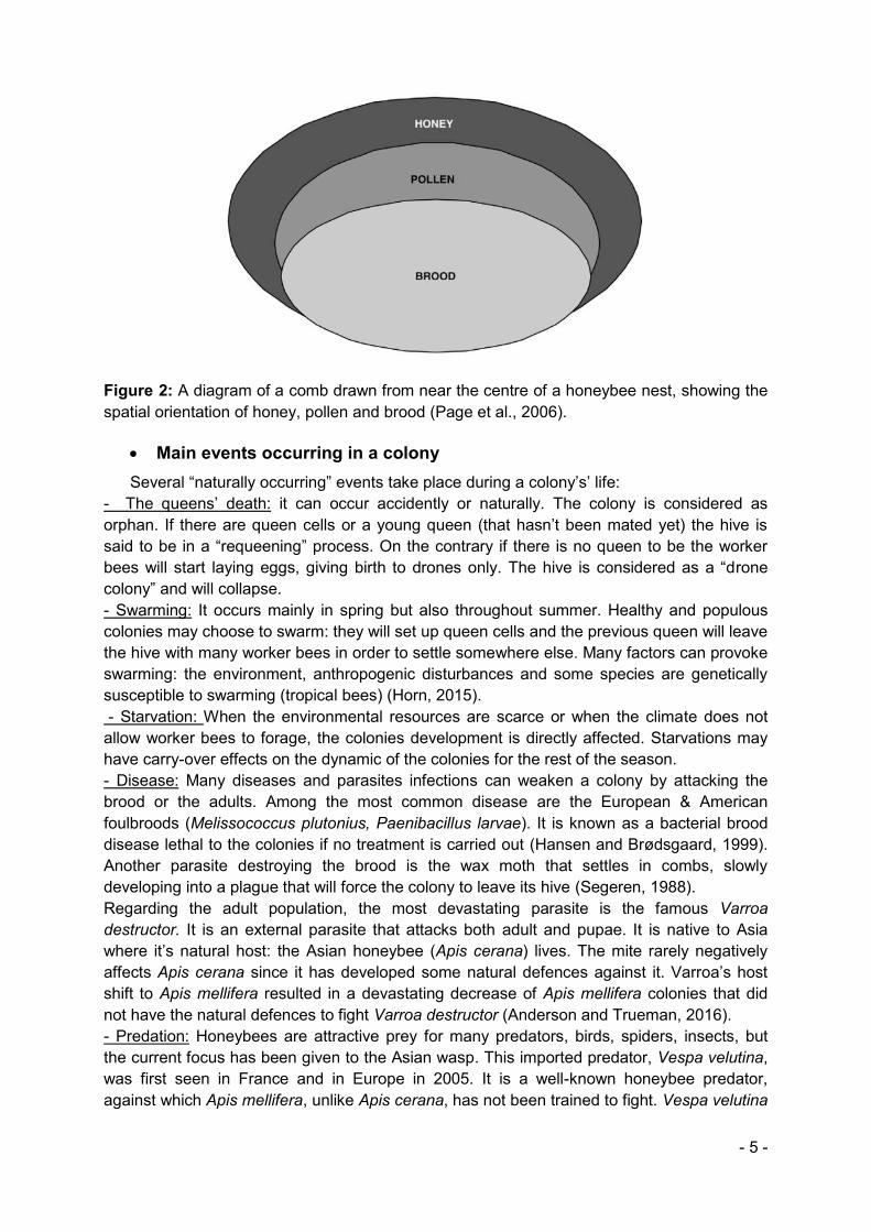
The colony is segmented into three parts: The adult population: Mainly found in the brood box it can also spread to the honey super when it is populous. The foraging bees come and go throughout the day, it mostly depends of the climate (temperature, precipitation, wind), the environment (resource availability) and the colony’s needs. The brood: It represents the reproductive investment of the colony, it is composed of all the future colony population: eggs, larvae, and pupae in capped brood. In the hive the brood nest is found in the middle on the central frames of the brood box (Page et al., 2006). This organisation allows the brood to stay in an environment with its optimal temperature (34-35°) and hygrometry (50-60%). The development of a worker bee lasts approximately 21 days (Rueppell et al., 2009). The honey reserves: composed of the nectar and pollen foraged by the worker bees. Nectar foragers returning to the hive pass their loads to younger bees through trophallaxis. It is then deposited in the combs where it will be processed by other bees into honey (Page et al., 2006). Returning pollen foragers store their loads in empty cells close to the area of the nest (figure 2).
- 5 -
Figure 2: A diagram of a comb drawn from near the centre of a honeybee nest, showing the spatial orientation of honey, pollen and brood (Page et al., 2006).
x Main events occurring in a colony Several “naturally occurring” events take place during a colony’s’ life:
- The queens’ death: it can occur accidently or naturally. The colony is considered as orphan. If there are queen cells or a young queen (that hasn’t been mated yet) the hive is said to be in a “requeening” process. On the contrary if there is no queen to be the worker bees will start laying eggs, giving birth to drones only. The hive is considered as a “drone colony” and will collapse. - Swarming: It occurs mainly in spring but also throughout summer. Healthy and populous colonies may choose to swarm: they will set up queen cells and the previous queen will leave the hive with many worker bees in order to settle somewhere else. Many factors can provoke swarming: the environment, anthropogenic disturbances and some species are genetically susceptible to swarming (tropical bees) (Horn, 2015). - Starvation: When the environmental resources are scarce or when the climate does not allow worker bees to forage, the colonies development is directly affected. Starvations may have carry-over effects on the dynamic of the colonies for the rest of the season. - Disease: Many diseases and parasites infections can weaken a colony by attacking the brood or the adults. Among the most common disease are the European & American foulbroods (Melissococcus plutonius, Paenibacillus larvae). It is known as a bacterial brood disease lethal to the colonies if no treatment is carried out (Hansen and Brødsgaard, 1999). Another parasite destroying the brood is the wax moth that settles in combs, slowly developing into a plague that will force the colony to leave its hive (Segeren, 1988). Regarding the adult population, the most devastating parasite is the famous Varroa destructor. It is an external parasite that attacks both adult and pupae. It is native to Asia where it’s natural host: the Asian honeybee (Apis cerana) lives. The mite rarely negatively affects Apis cerana since it has developed some natural defences against it. Varroa’s host shift to Apis mellifera resulted in a devastating decrease of Apis mellifera colonies that did not have the natural defences to fight Varroa destructor (Anderson and Trueman, 2016). - Predation: Honeybees are attractive prey for many predators, birds, spiders, insects, but the current focus has been given to the Asian wasp. This imported predator, Vespa velutina, was first seen in France and in Europe in 2005. It is a well-known honeybee predator, against which Apis mellifera, unlike Apis cerana, has not been trained to fight. Vespa velutina
- 6 -
feeds on honeybees, mostly forager bees, coming back to the hive with pollen and nectar. It beheads it’s pray, removes its wings and legs and brings the thorax back to its colony (Villemant et al., 2006).
x Colony nutrition Honeybee forage both pollen and nectar to meet their food requirements. Nectar or
honeydew represents their natural source of carbohydrates which allows them to meet their energetic expenses (Brodschneider and Crailsheim, 2010). Foragers collect nectar from the flowers, transport it to the hive and store it into sealed cells as honey. During the returning flight the transformation process of nectar into honey starts (Nicolson and Human, 2008). On the other hand, pollen is the only natural protein and lipid source for honeybees (Brodschneider and Crailsheim, 2010). It is consumed both by adults and larvae and is often consumed shortly after being brought back to the hive. Honeybees mix regurgitated nectar with pollen and store it in small quantities the mixture is called beebread. The weight of pollen in the amount of honey reserves of a bee colony is minor. Regardless of its weight pollen plays a key role in the accumulation of honey reserves. The pollen intake will influence the brood size and in fine the number of bee workers. Added to this indirect effect pollen influences positively bee health and is therefore crucial for the colony resilience to diseases (Avisse, 2014; Odoux et al., 2012; Manning, 2001).
x Pollination The impact of pollination service on agricultural production is widely acknowledged.
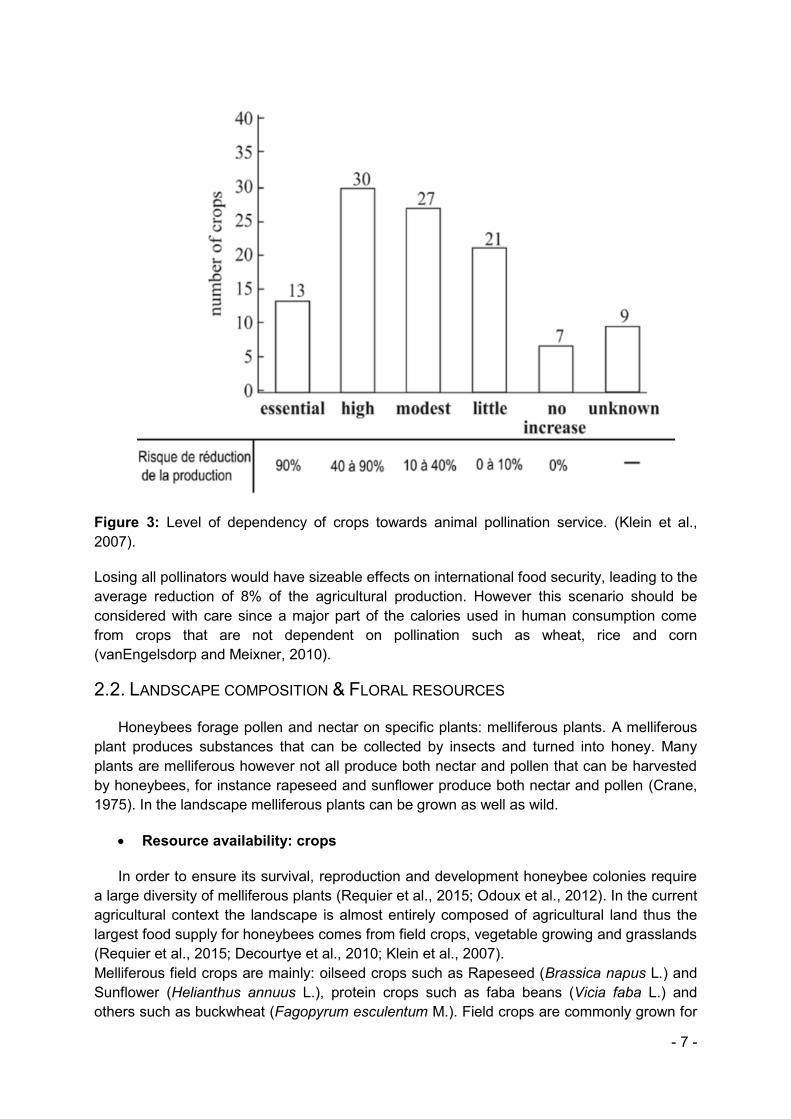
Pollination consists in pollen transfer from the anther to the stigma of a same or different flower. This is the first step in the fertilisation process. Among various dissemination agents different animals can contribute to this step among which the invertebrates and more specifically insects (Pouvreau et al., 2004). Honeybees are considered as the main insect pollinator in agricultural landscapes (Traité Rustica, 2002). This is due to the high number of individuals within one nest. As mentioned earlier in this report, in Europe 84%, meaning 150 grown crops, directly depend on insect pollination (S. Potts et al., 2010). According to Klein et al. (2007), at the international scale, 70% of the crops grown for human consumption, corresponding to 87 of the 124 crops grown directly for human consumption rely on animal pollination to produce and/or increase its production. The level of crop dependency to insect pollination varies from a crop to another (Corbet et al., 1991)(figure 3).
- 7 -
Figure 3: Level of dependency of crops towards animal pollination service. (Klein et al., 2007).
Losing all pollinators would have sizeable effects on international food security, leading to the average reduction of 8% of the agricultural production. However this scenario should be considered with care since a major part of the calories used in human consumption come from crops that are not dependent on pollination such as wheat, rice and corn (vanEngelsdorp and Meixner, 2010).
2.2. LANDSCAPE COMPOSITION & FLORAL RESOURCES
Honeybees forage pollen and nectar on specific plants: melliferous plants. A melliferous plant produces substances that can be collected by insects and turned into honey. Many plants are melliferous however not all produce both nectar and pollen that can be harvested by honeybees, for instance rapeseed and sunflower produce both nectar and pollen (Crane, 1975). In the landscape melliferous plants can be grown as well as wild.
x Resource availability: crops
In order to ensure its survival, reproduction and development honeybee colonies require a large diversity of melliferous plants (Requier et al., 2015; Odoux et al., 2012). In the current agricultural context the landscape is almost entirely composed of agricultural land thus the largest food supply for honeybees comes from field crops, vegetable growing and grasslands (Requier et al., 2015; Decourtye et al., 2010; Klein et al., 2007). Melliferous field crops are mainly: oilseed crops such as Rapeseed (Brassica napus L.) and Sunflower (Helianthus annuus L.), protein crops such as faba beans (Vicia faba L.) and others such as buckwheat (Fagopyrum esculentum M.). Field crops are commonly grown for
- 8 -
their grain on vast areas of land with minimum labour. Their blooming period occurs massively on a very short period of time. These crops are very attractive for beekeepers because of their high melliferous potential, however the intensive use of crop protection products endangers honeybees. Many vegetable plants such as pumpkins, carots, onions and many others, are melliferous despite their scarce blooming. Grasslands for animal consumption usually host several melliferous plants such as alfalfa (Medicago sativa L.) and white and red clover (Trifolium repens L., Trifolium pratense L.).
x Resource availability: wild floral resources
Are considered wild floral resources all the resources that are not cropped by humans: weeds, hedges, woods, grass strips, etc.
Starting from the end of the 2nd world war, European and National agricultural landscape have been strongly modified in order to meet the growing food requirements (Godfray et al., 2010). The regrouping of agricultural land led to farm expansion and a progressive decrease of semi natural habitats, hedges and grasslands that would only take up land needed for growing food (Rhoné, 2015). Land use intensification led to a shift in the spatial organisation of the landscape with obvious effects on agro biodiversity (Le Cœur et al., 2002). The fragmentation of the semi natural habitats, appropriate for nesting, feeding, mating, etc., causes the loss, in quality and quantity, of favourable habitats for biodiversity. All the processes combined: fragmentation, homogenisation, decrease of semi natural habitats, intensification progressively lead to the erosion of the agro biodiversity (Rhoné, 2015).
Grass strips: A strong diversity of wild floral resources can be encountered in the grass strips along the roads or the fields. However, their intensive mowing progressively reduces their occurrence and limits their attractiveness for pollinators.
Forest and Hedges: The removal of hedges was followed by the reduction and slow disappearance of plants producing pollen and nectar over the whole beekeeping season. Such as: blackthorn (Prunus spinosa L.), bramble (Rubus fructicosus L.), hawthorn (Crataegus sp.), etc. (Traité Rustica, 2002).
Crop weeds: Together with the landscape changes, agricultural practices became more intensive with an increase in pesticide use depriving pollinators from vital floral resources. For instance, cereal fields are not very attractive for honeybees, however the weeds they host: poppy (Papaver rhoeas L.) and cornflower (Centaurea cyanus L.) have widely been recognised as extremely interesting for the pollen supply of honeybee colonies (Requier et al., 2015). The intensive weeding and in particular the use of pesticide or the thorough cleaning of the seeds is leading to their decline, excluding them from the core of the field and reducing their growth to the field margins.
2.3. HONEYBEE DECLINE
- 9 -
Recent public and scientific interest for honeybees occurred when the sharp disappearance of worker bees from a colony was described as colony collapse disorder. From there on, research efforts have focused on improving colony health and management techniques, and identifying possible causes of colony collapse disorder. The population of honeybees are decreasing worldwide, this phenomena has been detected in Europe (S. G. Potts et al., 2010), many parts of the USA (Pettis and Delaplane, 2010) and in Asia (Oldroyd and Nanork, 2009). In Europe the number of colonies decreased from 21 million in 1970 to 15.5 million in 2007. Between 1985 and 2005, for 18 European countries the mean rate of colony losses reached 16% (figure 4). Considering the extent of this decline it was defined as: Colony Collapse Disorder (CCD) (Watanabe, 2008).
Figure 4: Change in colony numbers in 18 European countries. From 1965 - 1985 (a) and 1985 - 2005 (b). Grey arrows represent countries with an increase in number. Black arrows represent the countries with a decrease in number (S. Potts et al., 2010).
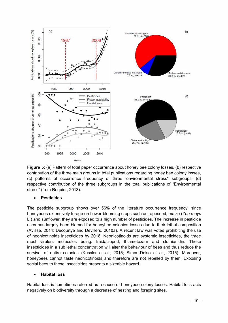
Since 1975, the number of publications related to honey bee colony losses has increased exponentially (Requier, 2013). To explain honeybee decline many factors have been proposed, they can be grouped into three broad categories of causes: Parasites and Pathogens, Genetic diversity and vitality and Environmental stress. This third group accounts for about 31.3% of the publications on honeybee colony losses, it is composed of three different subgroups: Pesticides, flower availability and habitat loss (figure 5).
- 10 -
Figure 5: (a) Pattern of total paper occurrence about honey bee colony losses, (b) respective contribution of the three main groups in total publications regarding honey bee colony losses, (c) patterns of occurrence frequency of three 'environmental stress" subgroups, (d) respective contribution of the three subgroups in the total publications of “Environmental stress” (from Requier, 2013).
x Pesticides
The pesticide subgroup shows over 56% of the literature occurrence frequency, since honeybees extensively forage on flower-blooming crops such as rapeseed, maize (Zea mays L.) and sunflower, they are exposed to a high number of pesticides. The increase in pesticide uses has largely been blamed for honeybee colonies losses due to their lethal composition (Avisse, 2014; Decourtye and Devillers, 2010a). A recent law was voted prohibiting the use of neonicotinoids insecticides by 2018. Neonicotinoids are systemic insecticides, the three most virulent molecules being: Imidacloprid, thiametoxam and clothianidin. These insecticides in a sub lethal concentration will alter the behaviour of bees and thus reduce the survival of entire colonies (Kessler et al., 2015; Simon-Delso et al., 2015). Moreover, honeybees cannot taste neonicotinoids and therefore are not repelled by them. Exposing social bees to these insecticides presents a sizeable hazard.
x Habitat loss
Habitat loss is sometimes referred as a cause of honeybee colony losses. Habitat loss acts negatively on biodiversity through a decrease of nesting and foraging sites.
- 11 -
x Flower availability
Though floral resources without doubt have an impact on the honeybee colony survival which is totally dependent on the honey reserves stored, there is no demonstrated evidence of a direct link between floral resources decrease and honey bee colony losses (Requier, 2013).
2.4. FLOWER AVAILABILITY AND HONEYBEE COLONY DYNAMICS IN INTENSIVE FARMLANDS
In an intensive cereal farming system, the reserve accumulation of honeybee colonies follows a seasonal pattern connected to the blooming period of the main mass flowering crops being rapeseed and sunflower. Honeybees forage on a wide diversity of flowers, however when the mass flowering crops are available they focus their foraging effort using them. Unfortunately, these mass flowering crops are highly seasonal and result in the occurrence of a ‘dearth period’, with a severe decrease in honey reserves (Requier et al., 2015), between the two peak flowering period of respectively rapeseed and sunflower (figure 6).
Figure 6: Inter-annual variations in the dynamics of hive brood chamber food reserves for 30 experimental colonies in years 2008-2011 (Odoux et al., 2014).
The severe food depletion during May and June compels honeybees to forage on wild floral resources.
x Wild floral resources & Reserve accumulation
- 12 -
Several landscape elements have been found to contribute favourably to the reserve of the colony such as the woody elements and the weeds in a landscape (Requier et al., 2015; Rhoné and Laffly, 2015). Requier et al. (2015) established that the woody elements and the weeds represent the major part of the pollen intake, more than 60% of the average pollen mass brought back to the hive (figure 7).
Figure 7: Botanical origin of pollen resources, expressed in biomass proportions (Requier et al., 2015)
Arable fields: Few studies have focused only on the dearth period, though some elements have been pointed out, such as the possible positive contribution of flax (Linum usitatissimum) and moha (Setaria italica) during this food shortage (Rivière, 2015; Le Gall, 2014). And on the other hand the negative effect of sunflower, blooming only later, taking up agricultural land without providing resources (Brenner, 2011). However later in the season, during its blooming period, sunflower represents a major resource for pollinators, accountable for the main honey harvest for beekeepers (Le Gall, 2014).
Weeds: Weeds constitute the bulk of the honeybee pollen diet during the dearth period (Requier et al., 2015). Arable weed species such as red poppy (Papaver rhoeas) act as an important food resource for biodiversity protection, in particular birds and insects (Bretagnolle and Gaba, 2015; Feuillet et al., 2008). However this central food resource is difficult to preserve considering that its optimal habitat is in crop fields (Fried et al., 2009). The occurrence of arable weeds has been declining as well as the species richness in which they occur. They are now disappearing from the core of the fields progressively confined to the field margins that act as refugee for weeds that can no longer survive in core fields (Fried et al., 2009). Thus edges and woody habitats are considered as crucial landscape elements when focusing on biodiversity and honeybee survival.
Urban areas:
- 13 -
Regarding some important features of the landscape, no clear consensus has been reached concerning its effect on the amount of reserve. Urban areas were proved to have a positive effect (Naug, 2009), whereas other authors (i.e. Lecocq et al., 2015) highlighted its negative correlation to the amount of resources in the hive.
Some authors focused on the amount of food produced around an apiary in order to determine what crops would provide most resources for honeybee. They showed that arable land is the poorest regarding the amount and diversity of nectar (Baude et al., 2016a). On the other hand, calcareous grassland, broadleaved woodland and neutral grassland are the habitats that produce the most nectar (quantity wise). Though the amount of available resources around the apiary could not yet be correlated to the amount of reserves in the hives (Rivière, 2015). We suspect a carry-over effect of the dearth period on the colony dynamics: the food shortage (May and June) would impact the colony later in the season.
x Wild floral resources and honeybee population
During the dearth period, other authors (e.g. Odoux et al., 2014) showed that the woody elements act as a buffer for the population decrease (figure 8), decrease which commonly occurs between the two mass flowering crops. Thus we could suspect that there would be more foraging bees and thus more food brought back to the hive when woody elements and weeds are abundant.
Figure 8: Influence of woody habitats on the colony size dynamics after oilseed rape period. The temporal axis was rescaled on each year's specific end date of oilseed rape blooming.
- 14 -
Curves show the expected colony size for the least and most forested environments, as defined by the median value of woody habitats surfaces measured within a 1.5 km radius from colonies (Odoux et al., 2014).
3. AIM OF THIS STUDY The ultimate aim of this study is to identify the main agricultural factors impacting
honey yields of bee colonies and in the long-term determine the sustainable agricultural practices allowing a favourable environment for the survival of pollinators. Throughout this study, despite the strong importance of pollen for honeybees, we chose to focus only on nectar. The weight of pollen bread in the reserve of the hive is marginal, in addition honey is made solely out of nectar. Thus when studying the link between the floral resources and the honey reserves we choose to consider nectar only.
The main objective of this study is to answer the following research question: How does spatiotemporal flower resource availability during the dearth period affect
honey reserves in the bee colonies? To do so we structure our work around four main hypotheses:
x 1st Hypothesis: The temporal variation in honey reserves follows the same pattern as
the temporal variation of nectar available resources.
Despite the widely recognized importance of floral resources, most studies focused on the quantity aspect of the floral resource rather than the temporal aspect. Considering the challenges that honeybees are facing regarding resource availability, it is important to address this temporal facet. Therefore, we wish to determine the temporal pattern of available floral resources and highlight the similarity it has with the honey reserve accumulation. This hypothesis would comfort the strong link between floral resources and honeybee survival.
x 2nd Hypothesis: The temporal variation of available floral resources (nectar) is different from one year to another.
The honey reserve accumulation suffers strong changes from one apicultural season to another. We wish to assess whether the floral resources suffer similar variations from one year to another.
x 3rd Hypothesis: Apiaries with higher amounts of floral resources are found having higher amounts of honey reserves in the brood chamber.
We suspect a strong correlation between the amount of available resources around the apiary and the amount of honey reserves. We attempt to confirm this idea and highlight differences between apiaries.
x 4th Hypothesis: Weeds are key floral resources during the dearth period. For this last hypothesis we focus on the weight of weeds in the constitution of honey reserves. We hope to confirm the importance of weed for honeybees either through their role as a buffer during the dearth period or their carry over effect on the colonies survival over winter.
The study area “Zone atelier Plaine & Val de Sèvre” is a long term ecological research network (LTER)(“Zone Atelier Plaine & Val de Sèvre,” n.d.), it is located south of Niort and encompasses 45 000 hectares of grain-growing plain. Half of the area is a Natura 2000 site, meaning that it contains rare wild species worth protecting (“Natura 2000,” n.d.). In
- 15 -
parallel an experimental design (ECOBEE) was set up in 2008, on the LTER, and is monitoring both ecological and environmental data concerning bee colonies since then. The ECOBEE data set can be analysed to investigate temporal and spatial issues in the ecology of honeybees in an intensive agro system (Odoux et al., 2014). The area is under a warm-temperate oceanic climate with regular summer dryness though bees rarely suffer from drought. Most of the environmental data concerns land use whereas other data sets focus on hedges and soil types. In 2016 we have eight years of data, for a total number of 400 monitored hives. Using this data set I performed spatial and statistical analyses. Throughout the apicultural season, data were collected every two weeks, visiting the hives and performing the measurements. I participated in this data collection for 2016, however the data collected this year were not used in the study due to time constraint. The knowledge gathered during this master thesis could later on be communicated to the agricultural and apicultural sectors, it could contribute to scientific publications and be used as a basis for further reflexion regarding the creation of future agro-environmental measures.
4. MATERIAL & METHODS The study of the interaction between landscape and honeybee colonies requires the
set-up of a thorough methodology. To do so, two main types of data exogenous and endogenous are needed. In order to structure this thesis work we set-up a time schedule (annex 1). The exogenous data enables the characterisation of the environment of the colonies for each of the 50 studied sites. This data is provided by the CNRS in charge of the LTER as digital maps with layers of information. When integrated into a geographic information system (QGIS), the data can be used as an explanatory variable for the colonies dynamic and development. The study of the vegetation enables the estimation of the floral resources available for the honeybees. The endogenous data is the result of in situ observation of the colonies through the ECOBEE design described below. These two data sets are first studied separately before being combined and analysed through statistical tests.
4.1. STUDY AREA AND EXPERIMENTAL DESIGN
The study was carried out in the Long-Term Ecological Research (LTER) Zone Atelier Plaine & Val de Sèvre in central western France. This area reaches 45 000 hectares and is being widely studied by researchers (figure 9). Amongst all the programs taking place in this area the ECOBEE experimental design (details in section 4.3.) through which the endogenous data is being collected.
- 16 -
Figure 9: Map of the LTER and its location in France (from Simon, 2015).
4.2. ASSESSING THE AVAILABLE RESOURCES
4.2.1 THE LAND USE IN THE LTER The digital maps provided by the CNRS give the land use records of all the LTER
over the years. The local agricultural landscape is mainly composed of arable land (average of 76% of the total land cover since 2008). A large part of the arable land is dedicated to cereal production (with 42% of the land cover), as well as sunflower (11%), maize (9%) and rapeseed (8%) production (figure 10).
Figure 10: Land cover of the LTER. Mean values from 2008 - 2015.
In this study we intend to assess the resources that each landscape elements provide for honeybees.
- 17 -
4.2.2 FORAGING BUFFER RADIUS In order to select solely the landscape elements that are within the reach of the
honeybee colonies we choose a foraging distance of 1 743 m around a hive. The scientific literature provides a wide range of values as for the foraging distance of honeybees in agricultural landscapes. However, few of these link the foraging distance to the landscape structure. One study investigated honeybee foraging in differentially structured landscapes. The overall mean foraging distance was 1526.1 ± 37.2 m however foraging distances for pollen collection was found to be larger in simple rather than in complex landscapes, reaching 1743 ± 71 m (Steffan-Dewenter and Kuhn, 2003). Considering the very simplified landscape in which the study takes place we accept 1743m to be the mean foraging distance for honeybees. Therefore, the studied sites were narrowed down to a 1743m buffer around the apiaries. The restricted time for this thesis oriented our choice to work on a single buffer size avoiding the dilution of the landscape information and allowing us to go deeper in the analysis. Thus each studied site has a similar surface of 954 hectares, corresponding to a circle of a 1743m radius with the hives in the centre (annex 2).
4.2.3. THE LANDSCAPE COMPARTMENTS We classify the landscape compartments according to the resource they represent for
honeybees, whether they are melliferous or not (table 1). The non-melliferous habitats are the habitats that do not produce any resources for honeybees or the habitats for which the melliferous potential could not be assessed through this study. For instance gardens and urban areas represent an interesting source of pollen and nectar (Naug, 2009) due to the presence of many ornamental plants that are then encountered during the pollen analysis. However, the data available does not allow us to measure the floral resources that these habitats provide.
Table 1: Classification of the landscape compartments of the LTER.
Melliferous habitat
Cultivated land Annual crops
Grasslands
Forest
Hedges
Road sides
Non-melliferous habitat Urban areas, orchard, gardens, built ups
4.2.4. POTENTIAL NECTAR PRODUCTION Unlike other authors (i.e. Janssens et al., 2006), we did not wish to predict the honey
production of an environment. On the contrary, we wish to assess the resources provided by various landscape compartments in order to compare them. We also wish to study how honeybee colonies respond to a variation in floral resources.
- 18 -
The calculation of the Potential Nectar Production is based on previous studies (i.e. Baude et al., 2016; Rhoné, 2015; Janssens et al., 2006) as well as various data base: for botanical surveys (farmland-2013), for melliferous potentials (Baude et al., 2016; Janssens et al., 2006; Koltowski, 2006, unpublished data). The general equation used is the following:
𝑷𝑵𝑷𝑨,𝑾 = ∑ (∑ 𝑆𝑠 × 𝐴𝑠 × 𝑚𝑝𝑠 × 𝑓𝑠,𝑊𝑠
)𝑙
x 𝑷𝑵𝑷𝑨,𝑾 : Potential Nectar Production of the apiary A per week W (in kg). x 𝒍 : Different landscape compartments (annual crops, grasslands, forest, hedges). x 𝒔 : Species producing nectar within landscape compartment l. x 𝑺𝒔: Surface occupied by the species s in the landscape compartment l (in ha). x 𝑨𝒔 ∶ Abundance/Coverage of the specie s in landscape compartment l (number of
plants/ha or %, details in the following sections). x 𝒎𝒑𝒔: Melliferous potential of the species s (in μg/flower/day in this case it will be
scaled up to kg/ha/week. In kg/ha/year, in this case it will be scaled down to kg/ha/week, see the details in the following sections).
x 𝒇𝒔,𝑾: Flowering of the species s (fluctuating from 1: peak blooming date to 0 no open flowers, see details below).
The 𝑷𝑵𝑷𝑨,𝑾 expressed in kg is based on the sum of the potential nectar production of all the species (s) within one landscape compartment (l). We kept only the species producing nectar and for which all the data needed were available. The surface 𝑺𝒍occupied by the landscape compartment l is a data provided by the CNRS through digital maps giving the land use records of all the LTER over the years. The abundance 𝑨𝒔 or in some cases the coverage of each species (s) is provided by various database which were collected in the LTER. The farmland database detailed later in this report provides a number of plants per hectare for annual crops and a coverage percentage for grasslands. For convenience, we consider here the number of flowers reduced to one single flower per plant. Other surveys performed by F.Requier provide a number of flowers per hectare. Thus the equation slightly changes from one landscape compartment to another. Various data sets were at our disposal for the melliferous potential 𝒎𝒑𝒔. Originating from Romania, Poland and England. England being the most complete dataset we chose to use their value (Baude et al., 2016a) when available. In the rare cases were it was not we calculated a mean melliferous potential value crossing data from Romania and Poland (Janssens et al., 2006; Koltowski, 2006; unpublished data). The flowering of the specie 𝒇𝒔,𝑾 is provided by the data base of the botanical team of INRA. Regular botanical surveys are performed around the LTER, they provide us with the beginning and end of the blooming period of the species. The values of 𝒇𝒔,𝑾 follow arbitrarily a triangular function (figure 11) taking one value per week, 1 during its peak blooming week and 0 at the margin of the species flowering span. Therefore, the Potential nectar production 𝑷𝑵𝑷𝑨,𝑾 only includes blooming species.
- 19 -
Figure 11: Schematic representation of flowering phenology modelling assuming a triangular function of flower blooming across the flowering season. Rapeseed blooming 𝒇𝒔,𝑾 in 2015.
In the general equation is not taken into account the attractiveness of the resource or any parameter related to the honeybee colony dynamics. Therefore, the potential nectar production calculated with the above formula is not a potential honey production.
4.3. ARABLE LAND
4.3.1. ANNUAL CROPS Rapeseed and Sunflower
The LTER is a grain growing plain, however oilseed crops such as sunflower and rapeseed respectively take up 11% and 8% of the land cover every year. These crops provide substantial floral resources for honeybees due to their massive blooming on a short period of time. We assess the resource that melliferous annual crops provide for honeybees on a weekly basis.
𝑷𝑵𝑷𝒍,𝑾 = 𝑆𝑙 × 𝑚𝑝𝑙 × 10−9 × 𝑛𝑏. 𝑓𝑙𝑜𝑤𝑒𝑟. ℎ𝑎 𝑙 × 𝑓𝑙,𝑊 x 𝑷𝑵𝑷𝒍,𝑾 : Potential Nectar Production of landscape compartment l in week W
x 𝑺𝒍: Surface covered by landscape compartment l. x 𝒎𝒑𝒍: Melliferous potential of landscape compartment l (in µg/flower/day). x 𝒇𝒍𝒐𝒘𝒆𝒓𝒊𝒏𝒈. 𝒔𝒑𝒂𝒏𝒍: Flowering span of one flower of the species l (in days). x 𝒏𝒃. 𝒇𝒍𝒐𝒘𝒆𝒓. 𝒉𝒂𝒍: Number of flowers per hectare for landscape compartment l. x 𝒇𝒍,𝑾: Flowering of the specie l (fluctuating from 1: peak blooming date to 0 no open
flowers, see details in the previous section). When looking at an annual crop there is a unique species composing landscape compartment l being the crop grown (for instance the landscape compartment: sunflower field is composed of a unique specie being sunflower). The melliferous potential 𝒎𝒑𝒍 is expressed in µg/flower/day, we convert it into kg (x 10-9). We scale it up to its annual production with the flowering span and finally scale it down to a weekly production with the number of blooming weeks (𝒏𝒃. 𝒃𝒍𝒐𝒐𝒎𝒊𝒏𝒈. 𝒘𝒆𝒆𝒌𝒔𝒍). This formula could not be used for all the annual crops.
Flax, Fababean and Pea
0
0,2
0,4
0,6
0,8
1
1,2
13 14 15 16 17 18 19 20
FLOW
ERIN
G %
WEEKS
- 20 -
The melliferous potential at the scale of the flower was not available for flax, fababean and field peas. These melliferous crops could not be put aside thus we used a melliferous potential data in kg/ha. This scaled up data induces a loss in precision. The formula is the following:
𝑷𝑵𝑷𝒍,𝑾 = 𝑆𝑙 × 𝑚𝑝𝑙 × 𝑓𝑙,𝑊
𝑛𝑏. 𝑏𝑙𝑜𝑜𝑚𝑖𝑛𝑔. 𝑤𝑒𝑒𝑘𝑠𝑙
x 𝑷𝑵𝑷𝒍,𝑾 : Potential Nectar Production of landscape compartment l in week W
x 𝑺𝒍: Surface covered by landscape compartment l. x 𝒎𝒑𝒍: Melliferous potential of landscape compartment l (in µg/flower/day). x 𝒇𝒍,𝑾: Flowering of the specie l (fluctuating from 1: peak blooming date to 0 no open
flowers, see details in the previous section). x 𝒏𝒃. 𝒃𝒍𝒐𝒐𝒎𝒊𝒏𝒈. 𝒘𝒆𝒆𝒌𝒔𝒍: Number of blooming weeks of landscape compartment l,
from the first flower blooming to the last (in weeks).
4.3.2. WEEDS IN ANNUAL CROPS Each crop provides honeybees with floral resources, either directly (rapeseed, flax
and sunflower), as detailed in the previous section, or indirectly through weeds that grow within their field. When measuring the resources provided by each of the crops we should not leave aside the wild floral resources growing together.
x 𝑷𝑵𝑷𝒍,𝑾: Potential nectar production of landscape compartment l in week W (in kg). x 𝑺𝑴𝒍: Surface of the field margins of landscape compartment l (in ha). x 𝑨𝑴𝒔,𝒍: Abundance of the species s in the field margin of landscape compartment l (in
number of plant/ha). x 𝑺𝑪𝒍: Surface of the field centre of landscape compartment l (in ha). x 𝑨𝑪𝒔,𝒍: Abundance of the species s in the centre of the field of landscape compartment
l (in number of plant/ha). x 𝒎𝒑𝒔: Melliferous potential of the species s (in μg/flower/day, we convert this value
into kg (x10−9)). x 𝒇𝒔,𝑾: Flowering of the species s (fluctuating from 1: peak blooming date to 0 no open
flowers, see details in section 4.2.4).
Surface calculation
We chose to distinguish the field margin from the core of the field due to the higher abundance of weeds in the field margin. We consider that the margin takes up 9m within the field. Indeed, weeds mainly spread within a field with agricultural vehicle, which the average maximum size can reach 9m.
𝑆𝑀𝑙 = 𝑃𝑙 × 9 × 0.0001 𝑆𝐶𝑙 = 𝐴𝑙 × 0.0001 − 𝑆𝑀𝑙
x 𝑆𝑀𝑙: Surface of the margin of landscape compartment l. x 𝑃𝑙: Perimeter of landscape compartment l (in m). x 𝑆𝐶𝑙: Surface of the centre of landscape compartment l (in ha).
- 21 -
x 𝐴𝑙: Area of the landscape compartment l (in m2). We consider the fields as having a rectangular shape, thus we substract from the margin surface the surface of the corners (figure 12).
Figure 12: Drawing illustrating the surface calculation methodology. Colour code: yellow – field core- green – field margin- red – field corners-.
Abundance calculation To calculate the mean abundance of each weed we use botanical data collected
through the CNRS database (Bota-Farmland 2013). The Bota-Farmland survey is performed in the LTER. Through this program the weed species and their abundance is recorded in different crop fields (cereal, sunflower, maize, rapeseed, faba beans, etc.). For each field the data is collected within 10 quadrats of 4m2 in the field core and 10 quadrats of 1m2 in the field margin. The data collected varies from 1 to 5, corresponding to a logarithmic (log10) scale. We replace this data by the geometric mean (table 2).
Table 2: Format of the Bota-Farmland data, the geometric mean are the values used in the further calculations.
Bota-Farmland data Log 10 Geometric mean 1 1 - 10 3.16 2 11 - 100 33.16 3 101 - 1 000 317.80 4 1 001 - 10 000 3 163.85 5 10 001 – 100 000 31 624.35 We select solely the data recorded from week 16 to 28, in order to have the main weed species occurring throughout the dearth period. We calculate the mean abundance for each species both in the field margin 𝑨𝑴𝒔 and in the field core 𝑨𝑪𝒔 for each different crop.
a) Mean abundance in the field Core
At the field scale:
𝐴𝐶𝑓𝑠 = ∑ 𝐴𝑠 × 10 000
40
x 𝑨𝑪𝒇𝒔 : Abundance in the Core, at the field scale, for species s in landscape compartment l (number of plants/ha).
x 𝑨𝒔: Abundance of species s within one quadrat of landscape compartment l (number of plants/4m2).
9m
- 22 -
We sum the recorded abundance within each quadrat for each species, this abundance is scaled down to a m2 value (divided by 40, 10 quadrats of 4 m2), and finally we scale up this data to a hectare value (multiplied by 10 000). This equation provides us with a mean abundance within each field. It then has to be brought to the crop scale.
At the landscape compartment scale:
𝐴𝐶𝑠,𝑙 = ∑ 𝐴𝐶𝑓𝑠
𝑛𝑏. 𝑓𝑖𝑒𝑙𝑑𝑙
x 𝑨𝑪𝒔,𝒍: Abundance of the species s in the field core of landscape compartment l (in number of plant/ha).
x 𝑨𝑪𝒇𝒔 : Abundance in the Core, at the field scale, for species s in landscape compartment l (number of plants/ha).
x 𝒏𝒃. 𝒇𝒊𝒆𝒍𝒅𝒍: Number of surveyed fields of landscape compartment l.
b) Mean abundance in the field Margin
At the field scale:
𝐴𝑀𝑓𝑠 = ∑ 𝐴𝑠 × 10 000
20
x 𝐴𝑀𝑓𝑠 : Abundance in the Margin, at the field scale, for species s in landscape compartment l (number of plants/ha).
x 𝑨𝒔: Abundance of species s within one quadrat of landscape compartment l (number of plants/4m2).
Following the same procedure at for the field core we sum the recorded abundance within each quadrat for each species. This abundance is scaled down to a m2 value (divided by 20, 5 quadrats of 4 m2), and finally we scale up this data to a hectare value (multiplied by 10 000). This equation provides us with a mean abundance within each field. It then has to be brought to the landscape compartment scale.
At the landscape compartment scale:
𝐴𝑀𝑠,𝑙 = ∑ 𝐴𝑀𝑓𝑠
𝑛𝑏. 𝑓𝑖𝑒𝑙𝑑𝑙
x 𝑨𝑴𝒔,𝒍: Abundance of the species s in the field margin of landscape compartment l (in number of plant/ha).
x 𝑨𝑴𝒇𝒔 : Abundance in the Margin, at the field scale, for species s in landscape compartment l (number of plants/ha).
x 𝒏𝒃. 𝒇𝒊𝒆𝒍𝒅𝒍: Number of surveyed fields of landscape compartment l.
Through these calculations we obtain a value for the abundance that is expressed in a number of plants per ha. We choose to consider one plant one flower.
4.3.3. GRASSLANDS The surface of grasslands in the LTER takes up on average 4% of the land cover. The equation used to assess the floral resources it provides is the following:
x 𝑷𝑵𝑷𝒍,𝑾: Potential nectar production of landscape compartment l in week W (in kg). x 𝑺𝑴𝒍: Surface of the field margins of landscape compartment l (in ha). x 𝑪𝑴𝒔: Coverage of the specie s in the field margin of landscape compartment l (in %).
- 23 -
x 𝑺𝑪𝒍: Surface of the field centre of landscape compartment l (in ha). x 𝑪𝑪𝒔: Coverage of the specie s in the centre of the field of landscape compartment l
(in %). x 𝒏𝒃. 𝒇𝒍𝒐𝒘𝒆𝒓𝒔: Number of flowers x 𝒎𝒑𝒔: Melliferous potential of the specie s (in kg/ha/year). x 𝒇𝒔,𝑾: Flowering of the specie s (fluctuating from 1: peak blooming date to 0 no open
flowers, see details in section 4.2.4). The previous equation is very similar to this of weeds in annual crops, the surface of the field margin and the centre is identical, the melliferous potential is in a different unit but the major change is for the percentage of coverage.
Percent cover calculation To calculate the mean coverage of each species we use botanical data collected
through the Bota-Farmland program (Bota-Farmland 2013). Unlike for annual crops, the bota-farmland program surveys the coverage (in %) for each species in grasslands. Within each field studied we use 20 quadrats of 1m2, 10 of which are placed in the field core and the 10 remaining placed in the field margin. We calculate the mean coverage for each species both in the field margin 𝑹𝑴𝒔 and in the field core 𝑹𝑪𝒔 for each different crop. The abundance is expressed in a percentage (%).
Number of flowers per unit area In order to convert the coverage percentage into a number of flowers per unit area we
use the database provided by Baude et al. It gives a number of flowers per m2, at the peak blooming date, when the surface is covered by the concerned specie, thus 100% coverage. Using a “rule of three” we convert our coverage percentage into a number of flowers.
4.3.4. GRASS STRIPS ON THE ROAD SIDE Grass strips often host a wide range of species for which honeybees carry an interest
whether it is for pollen or nectar. Knowing this we assess the melliferous potential provided by this landscape compartment. The equation is the following:
𝑷𝑵𝑷𝒍,𝑾 = ∑(𝑆𝑙 × 𝐴𝑠 × 𝑚𝑝𝑠 × 7. 10−9 × 𝑓𝑠,𝑊)𝑠
x 𝑷𝑵𝑷𝒍,𝑾: Potential Nectar Production of the landscape compartment l during week W (in kg).
x 𝑺𝒍: Surface covered by the landscape compartment l (in ha). x 𝑨𝒔 : Abundance of the species s in the landscape compartment l (in number of
flowers/ha). x 𝒎𝒑𝒔: Melliferous potential of the species s (in μg/flower/day, we scale up this value
to a weekly value (x7) and convert it into kg (x10−9)). x 𝒇𝒔,𝑾: Flowering of the species s in week W (fluctuating from 1: peak blooming date to
0 no open flowers, see details in section 4.2.4).
Abundance calculation
- 24 -
For this landscape compartment the botanical data at our disposal was surveyed by Fabrice Requier, a PhD student. He visited several sites on which he performed three transects of 50m. The data collected was in number of flowers. We use this data to calculate an average flower number per hectare for each species. Within the data base we select solely the data recorded between week 16 and 28 in order to have only species occurring during the dearth period.
𝐴𝑠 = ∑ 𝑎𝑠 × 10 000
(20 × 150)
x 𝑨𝒔: mean Abundance of the species s in the landscape compartment l (in number of flowers/ha).
x 𝒂𝒔 : Abundance of the species s recorded during the transect in the landscape compartment l (in number of flowers/ha).
We sum the recorded abundance within each transect for each species, this abundance is scaled down to a m2 value (divided by 20 and 150, 20 transects of 150 m each). We scale up this value to a number of flower/ha (multiplied by 10 000). This equation provides us with a mean abundance for each species s.
4.3.5. WOODS The literature review (presented in section 2.4.) brought to light the weight of forested
habitats on honeybee colony dynamics (i.e. Odoux et al., 2014). A forested habitat will buffer a honeybee population decrease during the dearth period. It is likely that this buffer is due to the floral resources forest habitats provide. In this section we intend to quantify the floral resources that woods provide. To do so we use the following equation:
𝑷𝑵𝑷𝒍,𝑾 = ∑ [(𝑆𝑀𝑙 × 𝐶𝑀𝑠 + 𝑆𝐶𝑙 × 𝐶𝐶𝑠) × 𝑚𝑝𝑠 × 𝑓𝑠,𝑊
𝑛𝑏. 𝑏𝑙𝑜𝑜𝑚𝑖𝑛𝑔. 𝑤𝑒𝑒𝑘𝑠𝑠]
𝑠
x 𝑷𝑵𝑷𝒍,𝑾: Potential nectar production of landscape compartment l in week W (in kg). x 𝑺𝑴𝒍: Surface of the forest margin (in ha). x 𝑪𝑴𝒔: Percentage of coverage of the species s in the forest margin (in %). x 𝑺𝑪𝒍: Surface of the forest centre (in ha). x 𝑪𝑪𝒔: Percentage of coverage of the species s in the centre of the forest (in %). x 𝒎𝒑𝒔: Melliferous potential of the species s (in kg/ha/year). x 𝒇𝒔,𝑾: Flowering of the species s (fluctuating from 1: peak blooming date to 0 no open
flowers, see details in section 4.2.4). x 𝒏𝒃. 𝒃𝒍𝒐𝒐𝒎𝒊𝒏𝒈. 𝒘𝒆𝒆𝒌𝒔𝒔: Number of blooming weeks of the specie s, from the first
blooming flower to the last (in weeks). Surface calculation
We chose to distinguish the forest margin from the centre of the forest due to the difference of the species these two habitats can host. We consider that the margin takes up 1m within the forest.
𝑆𝑀𝑙 = 𝑃𝑙 × 1 𝑆𝐶𝑙 = 𝐴𝑙 × 0.0001 − 𝑆𝑀𝑙
x 𝑆𝑀𝑙: Surface of the forest margin (in ha). x 𝑃𝑙: Perimeter of the forest (in m). x 𝑆𝐶𝑙: Surface of the forest centre (in ha).
- 25 -
x 𝐴𝑙: Area covered by the surface (in m2).
Coverage percentage calculation No botanical surveys are at our disposal regarding the forest specie composition. We
base our data on previous work that established a typical composition of the margin and the centre of the forest (Rivière, 2015)(table 3).
Table 3: Typical forest composition, centre and margin, in the LTER Plaine & Val de Sevre.
Specie Margin Coverage Centre Coverage Quercus robur L. 0 25 Fraxinus ornus L. 0 25 Acer pseudoplatanus L. 0 25 Prunus avium L. 0 25 Viburnum sp 10 0 Ligustrum sp 10 0 Sambucus sp 20 0 Cornus sanguinea L. 30 0 Rubus fructicosus L. 30 0
4.3.6. HEDGES The hedges occurring in the landscape play a key role in biodiversity conservation as
mentioned through the literature review. The surface that both woods and hedges occupy was obtained using QGIS (annex 3). They host a wide range of floral diversity among which melliferous plants. We intend to assess the amount of floral resources this habitat provides for honeybees.
𝑷𝑵𝑷𝒍,𝑾 = ∑(𝑆𝑙 × 𝐴𝑠 × 𝑚𝑝𝑠. 10−9 × 𝑓𝑠,𝑊)𝑠
x 𝑷𝑵𝑷𝒍: Potential Nectar Production of the landscape compartment l during week W (in kg).
x 𝑺𝒍: Surface covered by the landscape compartment l (in ha). x 𝑨𝒔 : Abundance of the specie s in the landscape compartment l (in number of
flowers/ha). x 𝒎𝒑𝒔: Melliferous potential of the specie s (in μg/flower/day), we convert this value
into kg (x10−9)). x 𝒇𝒔,𝑾: Flowering of the specie s in week W (fluctuating from 1: peak blooming date to
0 no open flowers, see details in section 4.2.4). The equation presented above is based on the same datasets as the calculation for grass strips on the roadsides. We use Fabrice Requier botanical surveys and use the same methodology as in section 4.3.4.
4.3. HONEYBEE RESERVE ACCUMULATION IN HONEYBEE COLONIES
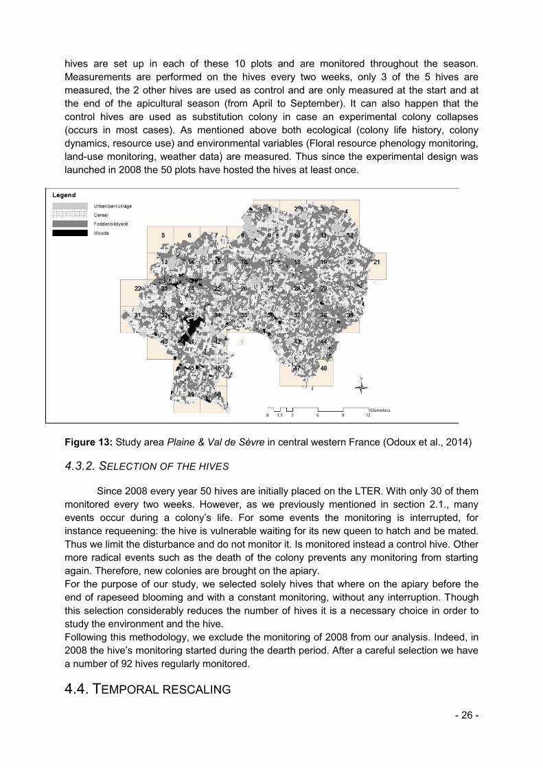
4.3.1 ECOBEE – HONEYBEE COLONY MONITORING DEVICE:
The Ecobee monitoring program was first launched in 2008. The LTER was divided into 50 plots of 10 km2, the size of each plot encompasses the main foraging distance of honeybees (figure 13). 10 plots are randomly chosen each year to be part of the study. 5
- 26 -
hives are set up in each of these 10 plots and are monitored throughout the season. Measurements are performed on the hives every two weeks, only 3 of the 5 hives are measured, the 2 other hives are used as control and are only measured at the start and at the end of the apicultural season (from April to September). It can also happen that the control hives are used as substitution colony in case an experimental colony collapses (occurs in most cases). As mentioned above both ecological (colony life history, colony dynamics, resource use) and environmental variables (Floral resource phenology monitoring, land-use monitoring, weather data) are measured. Thus since the experimental design was launched in 2008 the 50 plots have hosted the hives at least once.
Figure 13: Study area Plaine & Val de Sèvre in central western France (Odoux et al., 2014)
4.3.2. SELECTION OF THE HIVES
Since 2008 every year 50 hives are initially placed on the LTER. With only 30 of them monitored every two weeks. However, as we previously mentioned in section 2.1., many events occur during a colony’s life. For some events the monitoring is interrupted, for instance requeening: the hive is vulnerable waiting for its new queen to hatch and be mated. Thus we limit the disturbance and do not monitor it. Is monitored instead a control hive. Other more radical events such as the death of the colony prevents any monitoring from starting again. Therefore, new colonies are brought on the apiary. For the purpose of our study, we selected solely hives that where on the apiary before the end of rapeseed blooming and with a constant monitoring, without any interruption. Though this selection considerably reduces the number of hives it is a necessary choice in order to study the environment and the hive. Following this methodology, we exclude the monitoring of 2008 from our analysis. Indeed, in 2008 the hive’s monitoring started during the dearth period. After a careful selection we have a number of 92 hives regularly monitored.
4.4. TEMPORAL RESCALING
- 27 -
week
week
In order to compare the years between them we need to set up a time 0. Indeed, the blooming periods of rapeseed and sunflower sometimes face great changes from one year to another (figure 14).
15 16 17 18 19 20 21 22 23 24 25 26 27 28 29 30 31 2008 X X X X X X X X X X 2009 X X X X X X X X X X X X X X X 2010 X X X X X X X X X X X X 2011 X X X X X X X X X X X 2012 X X X X X X X X X X X X 2013 X X X X X X X X X X X 2014 X X X X X X X X X X 2015 X X X X X X X X X X X
Figure 14: Blooming calendar of rapeseed (orange) and sunflower (yellow) in the LTER Plaine & Val de Sèvre.
The temporal aspect is rescaled on each year’s specific beginning of sunflower blooming (figure 15).
-10 -9 -8 -7 -6 -5 -4 -3 -2 -1 0 1 2 3 4 5 6 2008 X X X X X X X X X X 2009 X X X X X X X X X X X X X X X 2010 X X X X X X X X X X X X 2011 X X X X X X X X X X X 2012 X X X X X X X X X X X X 2013 X X X X X X X X X X X 2014 X X X X X X X X X X 2015 X X X X X X X X X X X
Figure 15: Rescaling of the blooming calendar, rapeseed blooming period in orange, sunflower blooming period in yellow.
4.5 STATISTICAL ANALYSES In order to answer our hypotheses strong upstream work of data collection, treatment
and coding were performed. Using exclusively the R studio tool we created a script using the mathematical formulas presented in the sections above. The script calculates and combines all the nectar production of each landscape element for each year. This tool allowed us to perform all the further analysis described below.
4.5.1. SEASONAL PATTERN OF HONEY RESERVE AND FLORAL RESOURCE AVAILABILITY.
The upstream work provided us with the seasonal pattern of respectively, honey reserve and floral resource availability, over time. We wish to confirm, using statistics, what is visually identified: the mass of available nectar varies over the season. To do so we
- 28 -
performed non parametrical test (Kruskal Wallis) because the data was not normally distributed. This test gave use the information that at least one week was different from the others to go further we performed a post hoc test to calculate pairwise multiple comparisons between group levels. These tests are sometimes referred to as Nemenyi-tests.
Once we confirmed that the mass of available nectar varies over the season we visually compared the two seasonal patterns (honey reserves and mass of available nectar), identifying common peaks or troughs.
4.5.2. NECTAR CONTRIBUTION OF THE DIFFERENT LANDSCAPE COMPARTMENTS
We wish to bring to light the importance of the different landscape elements over the season. We divided the season into three main periods being the rapeseed blooming period, the dearth period and the sunflower blooming period. Using the previously mentioned statistical test: Kruskal Wallis followed by a Nemenyi on each of these three periods. These tests allow us to identify the major landscape elements. We use box plots to visually represent these results.
We look more specifically into the role of weeds compared to annual crops, we use a visual analysis using bar plots.
4.5.3. INTRA & INTER ANNUAL VARIATIONS IN THE MASS OF AVAILABLE NECTAR
We wish to assess firstly whether the mass of nectar available is different from one year to another and secondly whether the mass of nectar available is different from one apiary to another. To do so, we perform the previously mentioned statistical test: Kruskal Wallis followed by the post hoc Nemenyi test.
When looking at apiaries, to sharpen our analysis we focus on the dearth period only. When no statistical difference could be raised we visually identified the apiaries with the extreme data in order to study the difference in landscape composition of the two environments.
4.5.4. NECTAR AVAILABILITY AND HONEY RESERVES
Our final goal was to link the floral resources and the performance of the hive which in this study is resumed by the honey reserves. The first steps of our analysis are correlation tests between the two variables. We progressively improve our correlation by adapting the model: we remove the rapeseed blooming period during which the two variables do not match, we then force the intercept to 0 and use a polynomial correlation better fitting the data.
We erase the temporal differences between the years using a time 0 being the date of the first sunflower bloom. We visually observe a time laps between the sunflower peak and the honey reserves peak. We progressively align the data reaching an optimal correlation. In order to identify the variable on which the correlation works best we perform multiple correlation using mean, min, max and variation coefficient.
Finally, we link the honey reserves and available nectar of the two extreme apiaries that had been identified earlier. By doing so we wish to answer our hypothesis stating that the more floral resources in an apiary the more honey reserves it will accumulate.
5. RESULTS
- 29 -
5.1. SEASONAL PATTERN OF NECTAR AVAILABILITY AND HONEY RESERVES
The temporal pattern of both honey reserve and floral resources revealed a strong seasonal variation in the honey reserves and nectar availability (figure 16 and 17). The graphs below present data from week 15 to 30, corresponding to middle April – end of July.
Figure 16: Seasonal pattern of the floral resources (average mass of nectar available (in kg)) in one apiary (2008 – 2015). The vertical lines delineate the mass flowering periods of rapeseed and sunflower crops with the average dates for end of rapeseed blooming and beginning of sunflower. Each point represents the mass of nectar available (in kg) in one apiary.
Figure 17: Seasonal pattern of the average mass of honey reserves (in kg) in the apiary brood chamber (2009-2015). The vertical lines delineate the mass flowering periods of rapeseed and sunflower crops with the average dates for end of rapeseed blooming and
- 30 -
beginning of sunflower. Each point represents the average mass of honey reserves (in kg) in one apiary.
Nectar availability followed a strong bimodal pattern with two peaks (week 15 and week 30) preceded and followed by a period of lower nectar availability (figure 16). These two peaks coincide with the blooming periods of the two main mass flowering crops being successively rapeseed and sunflower. As for the period of lower availability it corresponds to the dearth period where resources are scarce.
As we strongly expected the honey reserves of an apiary followed a bimodal pattern with a poorly marked peak (week 20), almost inexistent and a sharper one (week 30) which coincides with the blooming of sunflower (figure 17). Therefore, honey reserves and the mass of available nectar peak simultaneously only during the sunflower blooming period.
5.2. NECTAR CONTRIBUTION OF THE DIFFERENT LANDSCAPE COMPARTMENTS
We assess the role played by the different landscape compartments over the beekeeping season. At the apiary scale, meaning within the 1743m buffer around the apiary. The below figure (figure 18) presents the nectar that is available on average per apiary (in kg), giving the detailed contribution of each landscape compartment over the beekeeping season.
Figure 18: Average seasonal contribution of the different landscape compartments in mass of available nectar (in kg) on average per apiary (2008-2015).
- 31 -
5.2.1 RAPESEED BLOOMING PERIOD
Rapeseed provides honeybees with massive amounts of nectar due to its high melliferous potential, its massive blooming and the wide surface it is grown on in the LTER. Thus when studying the rapeseed blooming period, no other landscape compartments can equal rapeseed’s nectar supply (figure 19 and annex 4). In week 16 (~3rd week of April), rapeseed is at its peak blooming period, its average nectar production on one apiary reaches 556 kg, the second biggest nectar producer at this same week is woods, with an average nectar supply of 21 kg. As we can see in the figure below, week 18 (1st week of May) is rather similar to week 16, indeed no landscape compartment equals the rapeseed nectar supply. Finally, week 20 (3rd week of May) follows the same pattern as the two previous weeks, however we can notice a slight increase in the nectar supply from woods. Despite this increase, rapeseed remains dominant.
Figure 19: Mass of available nectar (in kg) per apiary on average (2008-2015) in (a) week 16, (b) week 18 and (c) week 20 of each landscape compartment.
5.2.2 DEARTH PERIOD
During the dearth period floral resources are scarce, rapeseed blooming is over and sunflower blooming has not yet started. The most important landscape compartment during this time laps is weeds followed by grasslands and woods (figure 20 and annex 5). On average they respectively provide 50kg, 21.4 kg, 5.6kg of nectar during a week per apiary.
- 32 -
Figure 20: Mass of available nectar (in kg) in the different landscape compartments during the dearth period (week 23) per apiary on average.
5.2.3 SUNFLOWER BLOOMING PERIOD
Sunflower crops in the same way as rapeseed provide massive amount of nectar to which no other landscape compartment can compare. Indeed, during its peak blooming week, sunflower fields produce on average 682 kg of nectar within one apiary. During this period, grasslands represent the second biggest nectar supply with a production of 70.5 kg followed by weeds (48 kg) (figure 21 and annex 6).
Figure 21: Average mass of available nectar (in kg) on one apiary in each landscape compartment during the sunflower blooming (week 30).
- 33 -
We can easily conclude that the weight of semi natural habitats is marginal during the rapeseed and sunflower blooming. However, it becomes a substantial resource when these two oilseed crops are no longer blooming.
5.2.4 CONTRIBUTION OF THE LANDSCAPE COMPARTMENTS ON A SIMILAR SURFACE
We compare the nectar production (in kg) of each landscape element if it occupied a one-hectare surface (figure 22). This in order to identify landscape elements able to produce considerable quantities of nectar and that therefore should be set-up over larger surfaces.
Figure 22: mass of available nectar for one hectare (in kg/ha) produced by each landscape element per week during the three periods of the beekeeping season.
The above graph confirms the previous results being that during their respective blooming period, sunflower and rapeseed have a massive nectar production compared to the other landscape elements. Knowing this, it is interesting to focus solely on the dearth period. During the dearth period grassland is the most productive landscape element in terms of nectar with 0.53 kg/ha per week, followed by woods: 0.37 kg/ha/week and weeds: 0.26 kg/ha/week.
5.2.5. CULTIVATED CROPS VS WEEDS
We compare the nectar produced by weeds to the nectar provided by crops (figure 23). We can easily assess only visually that the contribution of weeds is marginal compared to what annual crops provide. For instance, week 27, annual crops provide 378 kg of nectar while weeds produce 50 kg of nectar. Despite this considerable difference annual crops do not provide any nectar during the dearth period unlike weeds.
- 34 -
Figure 23: Seasonal contribution of annual crops in mass of available nectar (in kg) average per apiary.
In this study 56 different melliferous weed species are taken into account. We identify the ten major weed species occurring during the dearth period (table4).
Table 4: Ten major weed species of the dearth period, mass of nectar (in kg) on average per apiary.
5.3. INTRA AND INTER ANNUAL VARIATIONS OF NECTAR AVAILABILITY
- 35 -
We identify the possible variations in floral resources between the years but more importantly within each year: are the floral resources different from one apiary to another?
5.3.1 INTER ANNUAL VARIATIONS
We assess whether the floral resource is different from one year to another, thus we compare the means of each year (on the studied period only). Since the data is not normally distributed we used a Kruskal Wallis test (p-value = 2.2e-16) indicating that one-year at least has different floral resource availability from the other years. To sharpen our analysis, we perform multiple comparisons between the years (Tukey and Kramer test).
The nectar availability throughout the season is identical from one year to another. It slightly fluctuates with the blooming periods of rapeseed and sunflower as we can see in 2009 when the resources are significantly different from all other years (p-value < 0.04, figure 24 and annex 7). Indeed, in 2009 the rapeseed blooming period spread over a large period of time, with the end date being the latest of the 8 years studied. In addition, that same year, the sunflower blooming was the earliest of the 8 years studied.
On the figure below we can also notice year 2011 as having an early sunflower bloom. However, no statistical differences were found between 2011 and the other years (other than 2009).
Figure 24: Seasonal pattern of the average mass of available nectar (in kg) in one apiary for each year. Light gray shading delineates mass-flowering periods of rapeseed and sunflower crops.
5.3.2 INTRA ANNUAL VARIATIONS
When studying the intra annual variations we looked at the seasonal nectar availability within the apiaries over the whole period (figure 25) and during the dearth period only (figure 26), since 2008 we count 80 apiaries. There are no significant statistical differences between the apiaries when we look at the dearth period only or at the whole season.
- 36 -
Figure 25: Seasonal pattern of the mass of available nectar (in kg) within each apiary.
Figure 26: Seasonal pattern of the mass of available nectar (in kg) within each apiary during the dearth period.
Despite the absence of statistical difference between the apiaries we can visually identify apiary 38 (in 2013) as having the maximum mass of nectar available through the whole dearth period (226 kg nectar) and apiary 22 (in 2011) as having the lowest mass of nectar available (44.36 kg nectar). The food resources of apiary 38 are more than five times
- 37 -
greater than those in apiary 22, though the p-value = 0.059 we may still consider the difference as substantial.
Contribution of the landscape elements in the two extreme apiaries
When looking at the contribution of the different landscape elements of these apiaries the main difference is in the contribution of grasslands (figure 27). During the dearth period, grasslands provide 2.23 kg nectar week 23 in apiary 22 whereas it provides 151.91 kg of nectar the same week in apiary 38.
Figure 27: Contribution of the different landscape compartments in mass of available nectar (in kg) in (a) apiary 38 and (b) apiary 22.
When studying solely two apiaries we might be treating with isolated cases, therefore we expand the analysis by considering as extreme the apiaries above the 3rd quartile and the apiaries below the 1st quartile.
- 38 -
Contribution of the landscape compartments of the apiaries within 3rd and 1st quartile
We isolate the apiaries for which the mass of available nectar is above the third quartile and the apiaries for which the mass of available nectar is below the 1st quartile. By doing so we isolate the “strongest” and “weakest” apiaries.
When looking at the contribution of the different landscape compartments of these apiaries (figure 28) we notice that whether the apiaries are strong or week the only landscape compartments providing nectar for honeybees are grasslands, weeds, woods and other melliferous crops.
The difference between the two groups of apiaries lies in the amount of nectar provided by these landscape compartments. Thus in the surface occupied by these landscape elements. For the “weak” apiaries in week 24 grasslands provide 29 kg of nectar whereas in strong apiaries, that same week grasslands provide 86 kg of nectar.
Are considered “strong”, apiaries that have more weeds, grasslands and woods in the apiary.
Figure 28: Seasonal pattern of the average mass of available nectar (in kg) in (a) the apiaries below the 1st quartile-“weak apiaries” and (b) the apiaries above the 3rd quartile – “strong apiaries”-.
- 39 -
5.4. NECTAR AVAILABILITY AND HONEY RESERVES
5.4.1 CORRELATION USING RAW DATA
The amount of honey reserves within a hive is positively correlated to the mass of available nectar in the apiary (p-value< 9.2e-16; figure 29). However, despite this strong statistical correlation, the mass of available nectar only explains 11.9 % of the honey reserves observed in the hive (adjusted R-squared = 0.1195).
Figure 29: Correlation graph of honey reserves (in kg) in the brood chamber and mass of available nectar (in kg) per apiary. Each point represents an observed value of honey reserve in a hive of a specific week correlated to the mass of nectar available within the buffer around the apiary at this same week.
We suspect that the correlation presented above is weakened by the collected data of the rapeseed blooming period. As stated in section 5.1., honey reserves and the mass of available nectar, peak simultaneously only after rapeseed blooming and during sunflower blooming. Therefore, when studying the correlation between these two variables we should only take into account the periods through which their patterns match. This period being, after the last blooming week of rapeseed. As expected in this correlation (figure 30) the mass of available nectar around the apiary explained now 21.4% of the honey reserves in the hives (p-value < 2.2e-16).
- 40 -
Figure 30: Correlation graph of honey reserves (in kg) in the brood chamber and mass of available nectar (in kg) in the apiary. Each point represents an observed value of honey reserve in a hive of a specific week correlated to the mass of nectar available within the buffer around the apiary at this same week. Are represented in this graph solely the data collected after the end of rapeseed blooming.
In order to improve the fit of the correlation we force the intercept to 0, assuming that no nectar available would mean no honey reserves. In parallel we apply a polynomial correlation which better fits this fluctuating data (figure 31). The p-value of the correlation is unchanged, however the adjusted R squared reaches 0.6216 meaning that the mass of available nectar explains 62.1% of the honey reserves measured in the hives.
Figure 31: Correlation graph of honey reserves (in kg) in the brood chamber and mass of available nectar (in kg) in the apiary. Each point represents an observed value of honey
- 41 -
reserve in a hive of a specific week correlated to the mass of nectar available within the buffer around the apiary at this same week. Are represented in this graph solely the data collected after the end of rapeseed blooming, the intersect is forced at 0 and we use a polynomial correlation to fit the data.
5.4.2 CORRELATION WITH TEMPORAL RESCALING
Time 0 identical for honey reserves and floral resources
The temporal variable was rescaled on each year’s specific beginning of sunflower blooming, both for honey reserves and for nectar availability (figure 32). We can visually assert that the increase in honey reserves, due to sunflower blooming, occurs with a slight time gap after the increase of floral resources. Despite the temporal rescaling the strength of the correlation stays unchanged with the mass of available nectar explaining 62.16% of the honey reserves.
a
- 42 -
Figure 32: Seasonal pattern of the average (a) mass of honey reserves (in kg) in the brood chamber per apiary (2009-2015) and (b) mass of nectar available (in kg) per apiary (2009 – 2015). The light gray shading delineates the mass flowering period of sunflower.
Temporal rescaling: suppression of a 1-week time gap
As stated above honey reserve increase occurs with a slight time gap after the available nectar increase. When this time gap is suppressed (of 1 week) the correlation slightly decreases, with the mass of available nectar explaining 47.64% of the honey reserves.
Temporal rescaling: suppression of a 2-week time gap
When this time gap is suppressed (of 2 week) the correlation reaches its optimum: the mass of available nectar explains 73,59% of the honey reserve in the hive (figure 33).
b
- 43 -
Figure 33: Correlation graph of honey reserves (in kg) in the brood chamber and mass of available nectar (in kg) in the apiary. Each point represents an observed value of honey reserve in a hive of a specific week correlated to the mass of nectar available within the buffer around the apiary at this same week. Are represented in this graph solely the data collected after the end of rapeseed blooming, the intersect is forced at 0 and we use a linear correlation to fit the data. The time 0 is rescaled with the suppression of a 2-week time gap.
5.4.3 CORRELATION USING THE OPTIMAL MODEL
Now that we have reached our optimal model, we test how different variables of honey reserves respond to floral resources (figure 34). The mean, maximum and minimum are strongly correlated to the mass of available nectar (with respectively R-squared: 0.7829, 0.7481, 0.7732) whereas the variation coefficient does not well respond to the correlation with a low adjusted R-squared of 0.1368.
- 44 -
Figure 34: Correlation graphs of (a) mean honey reserves (in kg), (b) maximum honey reserves, (c) minimum honey reserves and (d) variation coefficient of honey reserves, in the brood chamber with the mass of available nectar (in kg). Each point represents the mean/max/min/variation.coefficient for one apiary at a specific week.
5.4.4 PERFORMANCES OF THE HIVES IN THE TWO EXTREME APIARIES
When looking at the amount of honey reserves accumulated in the apiaries 38 and 22 mentioned in section 5.3.2. we can visually confirm that despite the higher amounts of floral resources available in apiary 38 compared to apiary 22 the amount of honey reserves does not follow the same trend (figure 35).
- 45 -
Figure 35: Average amount of honey reserves (in kg) in the brood chamber of a hive. The two extreme apiaries regarding floral resource availability.
5.4.5. PERFORMANCES OF THE HIVE IN THE TWO EXTREME QUARTILES When looking at the amount of honey reserves accumulated in the apiaries
considered as “strong” and “weak” (see section 5.3.2.: weak apiaries are those with available nectar below the 1st quartile, strong apiaries are those with available nectar above the 3rd quartile) we can visually conclude (figure 36) that despite the higher amounts of floral resources available in the “strong” apiaries compared to the “weak” apiaries, the amount of honey reserves does not follow the same strength.
Figure 36: Average amount of honey reserves (in kg) in the brood chamber of a hive in both the “strong” and the “weak” apiaries. Each point represents the average honey reserves per apiary.
- 46 -
6. DISCUSSION 6.1 SEASONAL PATTERN OF FLORAL RESOURCES.
As it was strongly expected and as it is mentioned in the literature, the amount of floral resources in the LTER follows a bimodal pattern driven by the blooming periods of the two main mass flowering crops (Odoux et al., 2014; Requier et al., 2015; Varis, 2000): rapeseed and sunflower respectively accounting for 94% and 85% of the available nectar at their peak blooming week. The abundance of resource that they offer has direct impacts on the dynamic of the colony. The high intake of food during the rapeseed blooming period induces a rapid demographic increase in the colony (Decourtye and Devillers, 2010b). These young and populous honeybee colonies are likely to suffer from food resource scarcity after the flowering ends.
The other landscape elements producing nectar cannot equal the nectar production of the two oilseed crops. However, their role may be when the massive blooming is over. The seasonal pattern confirms a two-month food shortage when rapeseed blooming is over and sunflower has not yet started. During this food shortage semi natural habitats are the only habitats able to provide food. This ability depends on the presence of wild plants in hedge rows, cereal fields, grass strips, grasslands, etc.
In the LTER the weeds represent the major nectar resource accounting for 63% of the total resources available at that time. Despite the huge nectar production of rapeseed and sunflower, wild floral resources such as weeds are crucial between the two blooming periods.
6.2 SEASONAL PATTERN OF HONEY RESERVE DOES NOT STRICTLY MATCH THE SEASONAL PATTERN OF FLORAL RESOURCES.
There is no strict coincidence between oilseed crop bloom and honey reserve. Floral resources and honey reserves peak simultaneously only during the sunflower blooming period. Other authors come to the conclusion that levels of nectar income are driven by the availability of the two dominant oilseed crops in intensive farmland habitats (Varis, 2000). In our study this statement is only confirmed during summer. Rapeseed and Sunflower crops account for respectively 10% of the crop surface, this suggests that rapeseed and sunflower are both available in the same amount for honeybees. Despite this similar availability honey bees neglect rapeseed in comparison to sunflower for nectar collection. One explanation as to why this might be the case is that the rapeseed blooming period coincides with the colony’s brood production period. The colonies brood size reaches its maximum early May thus honeybee colony’s priority during this period is not nectar collection but rather pollen collection. Pollen is mostly consumed by nursing bees in order for them to develop the glands that produce food for larvae (Haydak, 1970).
Therefore, the peak in floral resources during rapeseed blooming does not match a peak in honey reserves because honeybees prioritize pollen instead of nectar.
6.3 SEASONAL PATTERN OF FLORAL RESOURCES IS SIMILAR BETWEEN THE YEARS
As we strongly expected the nectar availability throughout the season is identical from one year to another. No clear differences can be found between the years because the land
- 47 -
use is strongly similar from one year to another thus the floral resources are identical over the years.
The unique sources of difference are the blooming dates. The blooming period varies from one year to another for each specie due to agriculture, climate, etc. We were not able to include this data variation for each species due to a lack of time and data.
Thus for each wild floral resources (weeds, hedges, woods) we used blooming dates recorded a specific year and applied these dates to all the years modelled. The blooming date variation are included exclusively for cultivated crops (rapeseed, sunflower, flax) for which the data was available.
This inaccuracy can partially explain the absence of difference between the years. Indeed, we can see that the only year different from the others: 2009, its difference relies in the large blooming period of both rapeseed and sunflower that year. Therefore, if the blooming periods were specific to each year we might have observed more differences between the years.
6.4 SIMILAR AMOUNTS OF FLORAL RESOURCES BETWEEN THE APIARIES
We expected to identify apiaries with stronger amounts of floral resources and conversely apiaries with low amount of floral resources due to the change in landscape composition. On the contrary no such difference could be statistically shown. As we cited in the literature previous studies highlighted the improved performance of hives that where in more forested habitats compared to those in least forested habitats. Thus we expected to confirm this statement.
What might begin to explain this counter result is the foraging buffer radius that I chose to use. As it is explained in section 4.2.2 we chose a foraging distance of 1 743m around the apiary. This distance was selected via data provided by the scientific literature (Steffan-Dewenter and Kuhn, 2003). Our aim was to solely select landscape element that where within the reach of the honeybee colonies. This chosen buffer radius could be too vast and therefore erase all the landscape composition differences between the apiaries. In further studies it would be interesting to study the amount of floral resources around an apiary at different buffer size.
6.5 WEEDS ARE THE MAIN FLORAL RESOURCE DURING THE DEARTH PERIOD
On average weeds produce 50kg of nectar over a week during the dearth period. It is the most productive landscape element at this period of the year. This nectar production is not the result of the contribution of a few species. Indeed, we identified the weed species contributing the most to the nectar production during the dearth period. We can conclude that there are no “major” weed species, thus it is weed communities in a broader sense that should be protected.
However, this nectar production is marginal compared to a weekly rapeseed (556 kg of nectar) and sunflower production (682 kg of nectar). Thus floral resources provided by weeds cannot be compared to the floral resources of the two main oilseed crops, however its temporal position makes it an important floral resource on which honeybees can forage in a very scarce period for flowers. The role of weeds should not be neglected when looking at the survival of honeybee colonies, they may represent a keystone element during the food shortage period (Decourtye et al., 2010) not only for nectar but also for their pollen diet. Indeed, a study by Requier et al. highlighted the great importance of weeds in the pollen diet of honeybees because of their continuous flowering phenology and their high species
- 48 -
richness (Requier et al., 2015). The presence of these weed species is clearly dependent on agricultural practices such as crop rotation, soil preparation and herbicide use. Weed conservation could be achieved through the reduction of pesticide use and more generally less intensive agricultural practices (Requier et al., 2015).
When modeling the amount of nectar provided by weeds, due to missing data, I arbitrarily chose one flower for one plant. It is a very inaccurate data considering that most plants produce complex inflorescences including many flowers. Thus the contribution of weeds in nectar production may be under-estimated in this study. In further studies it would be interesting to perform botanical surveys in order to assess the average number of flowers per plant during the peak blooming week. It would allow a more accurate modeling of the nectar production.
6.6 IMPORTANCE OF THE DIFFERENT LANDSCAPE COMPARTMENTS DURING THE DEARTH PERIOD
Besides weeds, other resources that we identified as being important during the dearth period are grasslands and woods. Indeed, when looking at the nectar production of each landscape element over one hectare, grasslands is the most productive landscape element at this period of the year. Added to this good productivity, the apiary with the higher amount of floral resources during the dearth period owed his consequent floral resources to the grassland contribution and the surface they occupied. However, floral resources provided by grasslands are very likely to be overestimated. Indeed, no mowing was taken into account. Despite this probable underestimate, a similar study performed in the United Kingdom revealed that calcareous and neutral grasslands and broadleaved woodland were the habitats that produce the greatest amount of nectar per unit area from the most diverse sources (Baude et al., 2016). Therefore, the beginning of a consensus around the importance of grasslands and woodlands is appearing. Woods is the second most nectar productive landscape element during the dearth period. It would be interesting to sharpen our analysis around this habitat. Since no botanical surveys were at our disposal we used a typical wood composition that had been established by previous master students. In further studies, botanical surveys could be performed in order to better assess the contribution of woods and likely better demonstrate its importance. An additional floral resource that has been left aside through this study are ornamental plants, it would be valuable to assess the nectar they produce over the dearth period.
6.7 APIARIES WITH HIGHER AMOUNT OF FLORAL RESOURCES ACCUMULATE MORE HONEY RESERVES
As we strongly expected the correlation between the amount of floral resources available around the apiary and the amount of honey reserves within the hive is solid. Indeed, the mass of nectar available around the apiary explains 73.59% of the amount of honey reserves. The role of nectar is empirically so obvious that beekeepers now provide supplements in the form of syrup.
We identified a two-week time laps between nectar availability and honey accumulation. This time laps is most probably the time needed for honeybees to find the resource, recruit working bees and collect the resource.
- 49 -
Despite the absence of statistical differences between the apiaries of the available floral resources, we could visually identify the apiary with the “maximum” and “minimum” floral resources throughout the dearth period. However, when linking the floral resources to the amount of honey the apiary with the higher amount of floral resources did not have the higher amount of honey reserve. This might be due to some over estimations of the nectar provided, in particular by grasslands.
Indeed, we reach similar conclusions when studying the group of apiaries with higher amount of floral resources and the group of apiaries with lower amount of floral resources. The conclusion being that higher amounts of floral resources do not automatically result in higher amounts of honey reserves.
6.8 LEADS TO PROTECT WILD FLORAL RESOURCES
The agri-environmental measures are often mentioned when discussing the increase of floral resources for pollinators (Decourtye et al., 2010; Requier et al., 2015). Baude et al compared five agri-environment schemes and the nectar they each provided. The agri-environment schemes being: wild bird seed mixtures, enhanced grass buffer strip, nectar flower mixture, haymaking supplement and species rich semi-natural grasslands. Nectar flower mixtures thus appeared to have the highest nectar productivity value. Though this productivity is comparable to hedgerows when looking at the annual nectar productivity per unit area, they cover a smaller area and therefore contribute far less to the nectar provision. Thus hedgerows seem to be the most productive feature of the environment, when the set-up of hedgerows is not possible enhancing the development of improved grasslands would greatly improve the nectar productivity of the environment and thus the pollinators survival (Baude et al., 2016).
6.7 LIMITS AND IMPROVEMENTS
The innovative approach of this study lies in the methodology developed. Indeed, assessing the available nectar of an environment is a rather new approach. Several changes should be taken into account to improve this methodology. Firstly, many data are available for melliferous potential over the scientific literature, but few of these data sets deal with a wide range of plants in agricultural habitat with a homogeneous method. We chose to use the most exhaustive data set we could find (Baude et al. 2016), however the constitution of a large database from a long term regional survey in field conditions within a large species range stays necessary. Such a database would allow us to take into account a larger number of species (especially regarding weeds). Moreover, the melliferous potential should be considered carefully. Indeed, its’ values strongly fluctuate with the temperature, the hour of the day (unpublished sources) and the methodology used to extract the nectar from the flower.
Other researchers such as Janssens et al., developed a tool to assess the potential honey production of an environment. The aim of our study differs, Janssens provides beekeepers with a tool to predict how much honey they can make from an environment, our study solely assesses the available nectar of an environment. Thus Janssens pushes the methodology further by adding other parameters such as: the attractivity of the floral resource and its
- 50 -
distance to the hive (Janssens et al., 2006). Nevertheless, the melliferous potential data used by Janssens derives from multiple studies performed in various countries, thus the data is hardly comparable. Moreover, the melliferous potential is used at the scale of a field. During our study we noticed that using the melliferous potential at the flower scale allowed us to gain in precision.
Another similar study, performed in England by Baude et al. assesses the nectar available in different environments (Baude et al., 2016). This study is the most exhaustive and accurate research we encountered in the literature. However, they do not link this available nectar to the honeybee colonies performances.
To conclude, if further studies where to be carried out in this field, an exhaustive dataset of the melliferous potential of a large number of species would be needed. Additional botanical surveys should be performed in order to have the number of open flowers of the different species, but also in order to establish a more accurate typical wood composition.
- 51 -
CONCLUSION
The coupled land use-colony monitoring data on a large scale provides a strong background to test for different environmental factors related with food resources and other stressors. Even if much research is left to be done to improve the assessment of the floral resources that each habitat provides, this study highlights that these resources are essential for honeybees.
It is urgent to preserve current semi natural habitats in farmlands (hedgerows, woodlands, ponds, ditches) and more specifically the weed community that plays a key role in the food supply during the dearth period.
Through agro environmental measures, nectar flower mixtures should be set up. These schemes should allow farmers to derive an agronomic benefit: the enhanced pollination service balancing the costs of introducing floral schemes. Thus studies are needed to assess the effectiveness of floral enhancement for pollinators. The set-up of floral fallows has been the subject of several research programs. However, it may be hard for farmers to understand how the enhanced pollination counter balances the cost of the seeds and maintenance that they had to set-up a floral fallow. Protecting valuable species for honeybees could also come with a better management of the pesticides.
The findings of this study are a valuable first step to understand how landscape influences honeybee and how the different landscape elements contribute to the maintenance of colony viability. Further studies should be performed to identify the most efficient schemes enhancing floral resources for honeybee.
http://entnemdept.ufl.edu/creatures/misc/bees/varroa_mite.htm Avisse, I., 2014. Grand traité des miels, Le Sureau. ed. Le Sureau - Apidis. Baude, M., Kunin, W.E., Boatman, N.D., Conyers, S., Davies, N., Gillespie, M.A.K., Morton,
R.D., Smart, S.M., Memmott, J., 2016a. Historical nectar assessment reveals the fall and rise of floral resources in Britain. Nature 530, 85–88. doi:10.1038/nature16532
Baude, M., Kunin, W.E., Boatman, N.D., Conyers, S., Davies, N., Gillespie, M.A.K., Morton, R.D., Smart, S.M., Memmott, J., 2016b. Historical nectar assessment reveals the fall and rise of floral resources in Britain. Nature 530, 85–88. doi:10.1038/nature16532
Brenner, J., 2011. Spatiotemporal variation in honey reserves within agricultural landscapes (Master thesis (M2)). Georg-August-Universität Göttingen.
Bretagnolle, V., Gaba, S., 2015. Weeds for bees? A review. Agron. Sustain. Dev. 35, 891–909. doi:10.1007/s13593-015-0302-5
Brodschneider, R., Crailsheim, K., 2010. Nutrition and health in honey bees. Apidologie 41, 278–294. doi:10.1051/apido/2010012
Carvalheiro, L.G., Veldtman, R., Shenkute, A.G., Tesfay, G.B., Pirk, C.W.W., Donaldson, J.S., Nicolson, S.W., 2011. Natural and within-farmland biodiversity enhances crop productivity: Weeds maximize nature benefits to crops. Ecol. Lett. 14, 251–259. doi:10.1111/j.1461-0248.2010.01579.x
Centre d’Etude Biologique de Chizé - Equipes de recherche [WWW Document], n.d. . cebc.cnrs.fr. URL http://www.cebc.cnrs.fr/Frecherche/equipes.htm
Corbet, S., Williams, I., Osborne, J., 1991. Bees and the pollination of crops and wild flowers in the European Community. Bee World 72, 47–59.
Crane, E., 1999. The world history of beekeeping and honey hunting. Routledge, New York. Crane, E., 1975. Honey. A comprehensive survey. Decourtye, A., Devillers, J., 2010a. Ecotoxicity of Neonicotinoid Insecticides to Bees, in:
Thany, SH (Ed.), INSECT NICOTINIC ACETYLCHOLINE RECEPTORS, Advances in Experimental Medicine and Biology. pp. 85–95.
Decourtye, A., Devillers, J., 2010b. Ecotoxicity of Neonicotinoid Insecticides to Bees, in: Thany, SH (Ed.), INSECT NICOTINIC ACETYLCHOLINE RECEPTORS. pp. 85–95.
Decourtye, A., Mader, E., Desneux, N., 2010. Landscape enhancement of floral resources for honey bees in agro-ecosystems. Apidologie 41, 264–277.
EFSA, 2009. Bee mortality and Bee surveillance in Europe (Scientific report). Feuillet, D., Odoux, J.-F., Aupinel, P., Lamy, H., Moreau, N., Roucher, L., Souche, T., 2008.
Evolution floristique et physico-chimique des pollens récoltés au cours de l’année 2006 sur le site de l’INRA du Magneraud. Bulletin Technique Apicole OPIDA 35, 20–26.
Fried, G., Petit, S., Dessaint, F., Reboud, X., 2009. Arable weed decline in Northern France: Crop edges as refugia for weed conservation? Biol. Conserv. 142, 238–243. doi:10.1016/j.biocon.2008.09.029
Hansen, H., Brødsgaard, C.J., 1999. American foulbrood: a review of its biology, diagnosis and control. Bee World 80, 5–23. doi:10.1080/0005772X.1999.11099415
Histoire de la PAC [WWW Document], n.d. URL https://www.supagro.fr/capeye/histoire-de-la-pac/ (accessed 3.29.16).
Horn, H., 2015. Beekeeping in the tropics. INRA, 2012. Who we are [WWW Document]. URL http://institut.inra.fr/en (accessed 4.8.16). Janssens, X., Bruneau, É., Lebrun, P., 2006a. Prévision des potentialités de production de
miel à l’échelle d’un rucher au moyen d’un système d’information géographique. Apidologie 37, 351–365. doi:10.1051/apido:2006006
Janssens, X., Bruneau, É., Lebrun, P., 2006b. Prévision des potentialités de production de miel à l’échelle d’un rucher au moyen d’un système d’information géographique. Apidologie 37, 351–365. doi:10.1051/apido:2006006
Klein, A.-M., Vaissiere, B.E., Cane, J.H., Steffan-Dewenter, I., Cunningham, S.A., Kremen, C., Tscharntke, T., 2007. Importance of pollinators in changing landscapes for world crops. Proc. R. Soc. B Biol. Sci. 274, 303–313. doi:10.1098/rspb.2006.3721
Koltowski, Z., 2006. Honey potential of plants growing under Poland’s condition. Le Cœur, D., Baudry, J., Burel, F., Thenail, C., 2002. Why and how we should study field
boundary biodiversity in an agrarian landscape context. Agric. Ecosyst. Environ. 89, 23–40. doi:10.1016/S0167-8809(01)00316-4
Le Gall, N., 2014. Evolution spatiotemporelle des récoltes de miel dans un paysage agricole (IUT La Roche-sur-Yon). Université de Nantes.
Le traité Rustica de l’apiculture: 1000 conseils clés, 2002. . Rustica, Paris. Lecocq, A., Kryger, P., Vejsnæs, F., Bruun Jensen, A., 2015. Weight Watching and the Effect
of Landscape on Honeybee Colony Productivity: Investigating the Value of Colony Weight Monitoring for the Beekeeping Industry. PLOS ONE 10, e0132473. doi:10.1371/journal.pone.0132473
Manning, R., 2001. Fatty acids in pollen: a review of their importance for honey bees. Bee World 82, 60–75.
Natura 2000 - Ministère de l’Environnement, de l’Energie et de la Mer [WWW Document], n.d. . Dev.-Durablegouvfr. URL http://www.developpement-durable.gouv.fr/-Natura-2000,2414-.html (accessed 3.29.16).
Naug, D., 2009. Nutritional stress due to habitat loss may explain recent honeybee colony collapses. Biol. Conserv. 142, 2369–2372. doi:10.1016/j.biocon.2009.04.007
Nicolson, S.W., Human, H., 2008. Bees get a head start on honey production. Biol. Lett. 4, 299–301. doi:10.1098/rsbl.2008.0034
Odoux, J.-F., Aupinel, P., Gateff, S., Requier, F., Henry, M., Bretagnolle, V., 2014. ECOBEE: a tool for long-term honey bee colony monitoring at the landscape scale in West European intensive agroecosystems. J. Apic. Res. 53, 57–66. doi:10.3896/IBRA.1.53.1.05
Odoux, J.-F., Feuillet, D., Aupinel, P., Loublier, Y., Tasei, J.-N., Mateescu, C., 2012. Territorial biodiversity and consequences on physico-chemical characteristics of pollen collected by honey bee colonies. Apidologie 43, 561–575. doi:10.1007/s13592-012-0125-1
- 54 -
Oldroyd, B.P., Nanork, P., 2009. Conservation of Asian honey bees. Apidologie 40, 296–312. doi:10.1051/apido/2009021
Ollerton, J., Winfree, R., Tarrant, S., 2011. How many flowering plants are pollinated by animals? Oikos 120, 321–326. doi:10.1111/j.1600-0706.2010.18644.x
Page, R.E., Scheiner, R., Erber, J., Amdam, G.V., 2006. The Development and Evolution of Division of Labor and Foraging Specialization in a Social Insect (Apis mellifera L.), in: Current Topics in Developmental Biology. Elsevier, pp. 253–286.
Persson, A.S., Olsson, O., Rundlöf, M., Smith, H.G., 2010. Land use intensity and landscape complexity—Analysis of landscape characteristics in an agricultural region in Southern Sweden. Agric. Ecosyst. Environ. 136, 169–176. doi:10.1016/j.agee.2009.12.018
Pettis, J.S., Delaplane, K.S., 2010. Coordinated responses to honey bee decline in the USA. Apidologie 41, 256–263. doi:10.1051/apido/2010013
Potts, S., Roberts, S., Dean, R., Marris, G., Brown, M., Jones, R., Neumann, P., Settele, J., 2010. Declines of managed honey bees and beekeepers in Europe. J. Apic. Res. 49, 15. doi:10.3896/IBRA.1.49.1.02
Pouvreau, A., Pham-Delègue, M.-H., Office pour les insectes et leur environnement (France), 2004. Les insectes pollinisateurs. Delachaux et Niestlé, Paris.
Requier, F., 2013. Dynamique spatio-temporelle des ressources florales et écologie de l’abeille domestique en paysage agricole intensif. Université de Poitiers.
Requier, F., Odoux, J.-F., Tamic, T., Moreau, N., Henry, M., Decourtye, A., Bretagnolle, V., 2015. Honey bee diet in intensive farmland habitats reveals an unexpectedly high flower richness and a major role of weeds. Ecol. Appl. 25, 881–890.
Rhoné, F., 2015. L’abeille à travers champs: quelles intéractions entre Apis mellifera L et le paysage agridole? : le rôle des structures paysagères ligneuses dans l’apport de ressources trophiques et leurs répercussions sur les traits d’histoire de vie des colonies. Toulouse 2, Toulouse.
Rhoné, F., Laffly, D., 2015. Evolution des ressources nectarifères et pollinifères mobilisées par l’abeille domestique: le rôle de la composante ligneuse, in: Abeilles et Paysages: Enjeux Apicoles et Agricoles. Quae.
Rivière, C., 2015. Impact des pratiques agricoles sur l’abeille domestique en plaine agricole (Master thesis (M2)). Université de Poitiers.
Rueppell, O., Kaftanouglu, O., Page Jr., R.E., 2009. Honey bee (Apis mellifera) workers live longer in small than in large colonies. Exp. Gerontol. 44, 447–452. doi:10.1016/j.exger.2009.04.003
Segeren, P., 1988. Beekeeping in the tropics, Agromisa Foundation. ed. Wageningen. Simon, E., 2015. Interactions between farming practices and pollinating insects in a network
of bee-favouring cropping systems DEPHY - Abeille project (Master thesis (M2)). Simon-Delso, N., Amaral-Rogers, V., Belzunces, L.P., Bonmatin, J.M., Chagnon, M., Downs,
C., Furlan, L., Gibbons, D.W., Giorio, C., Girolami, V., Goulson, D., Kreutzweiser, D.P., Krupke, C.H., Liess, M., Long, E., McField, M., Mineau, P., Mitchell, E.A.D., Morrissey, C.A., Noome, D.A., Pisa, L., Settele, J., Stark, J.D., Tapparo, A., Van Dyck, H., Van Praagh, J., Van der Sluijs, J.P., Whitehorn, P.R., Wiemers, M., 2015. Systemic insecticides (neonicotinoids and fipronil): trends, uses, mode of action and metabolites. Environ. Sci. Pollut. Res. 22, 5–34. doi:10.1007/s11356-014-3470-y
- 55 -
Steffan-Dewenter, I., Kuhn, A., 2003. Honeybee foraging in differentially structured landscapes. Proc. R. Soc. B Biol. Sci. 270, 569–575. doi:10.1098/rspb.2002.2292
Tardieu, V., 2015. Quelles avancées depuis L’étrange silence des abeilles ?, in: Abeilles et paysages: Enjeux apicoles et agricoles. pp. 11–12.
vanEngelsdorp, D., Meixner, M.D., 2010. A historical review of managed honey bee populations in Europe and the United States and the factors that may affect them. J. Invertebr. Pathol. 103, S80–S95. doi:10.1016/j.jip.2009.06.011
Varis, A.-L., 2000. Influence of changes in crop cultuvation areas on pollen contents of honey. Agricultural and food science in Finland 9, 253–257.
Villemant, C., Haxaire, J., Streito, J., 2006. La découverte du Frelon asiatique Vespa velutina, en France. Insectes 4.
Watanabe, M.E., 2008. Colony Collapse Disorder: Many Suspects, No Smoking Gun. BioScience 58, 384. doi:10.1641/B580503
Zone Atelier Plaine & Val de Sèvre [WWW Document], n.d. . za.plainevalsevre.cnrs.fr. URL http://www.za.plainevalsevre.cnrs.fr/ (accessed 3.29.16).
- 56 -
TABLE OF FIGURES FIGURE 1: STRUCTURE OF A DADANT HIVE. ........................................................................................................................ - 4 - FIGURE 2: A DIAGRAM OF A COMB DRAWN FROM NEAR THE CENTRE OF A HONEYBEE NEST, SHOWING
THE SPATIAL ORIENTATION OF HONEY, POLLEN AND BROOD (PAGE ET AL., 2006). .......................... - 5 - FIGURE 3: LEVEL OF DEPENDENCY OF A CROP TOWARDS POLLINATION SERVICE.. ...................................... - 7 - FIGURE 4: CHANGE IN COLONY NUMBERS IN 18 EUROPEAN COUNTRIES. FROM 1965 - 1985 (A) AND
1985 - 2005 (B). GREY ARROWS REPRESENT COUNTRIES WITH AN INCREASE IN NUMBER. BLACK ARROWS REPRESENT THE COUNTRIES WITH A DECREASE IN NUMBER.(S. POTTS ET AL., 2010).- 9 -
FIGURE 5: (A) PATTERN OF TOTAL PAPER OCCURRENCE ABOUT HONEY BEE COLONY LOSSES, (B) RESPECTIVE CONTRIBUTION OF THE THREE MAIN GROUPS IN TOTAL PUBLICATIONS REGARDING HONEY BEE COLONY LOSSES, (C) PATTERNS OF OCCURRENCE FREQUENCY OF THREE 'ENVIRONMENTAL STRESS" SUBGROUPS, (D) RESPECTIVE CONTRIBUTION OF THE THREE SUBGROUPS IN THE TOTAL PUBLICATIONS OF “ENVIRONMENTAL STRESS”. ...................................... - 10 -
FIGURE 6: INTER-ANNUAL VARIATIONS IN THE DYNAMICS OF HIVE BROOD CHAMBER FOOD RESERVES FOR 30 EXPERIMENTAL COLONIES IN YEARS 2008-2011 (ODOUX ET AL., 2014). .............................. - 11 -
FIGURE 7: BOTANICAL ORIGIN OF POLLEN RESOURCES, EXPRESSED IN BIOMASS PROPORTIONS (REQUIER ET AL., 2015) .................................................................................................................................................... - 12 -
FIGURE 8: INFLUENCE OF WOODY HABITATS ON THE COLONY SIZE DYNAMICS AFTER OILSEED RAPE PERIOD. THE TEMPORAL AXIS WAS RESCALED ON EACH YEAR'S SPECIFIC END DATE OF OILSEED RAPE BLOOMING. CURVES SHOW THE EXPECTED COLONY SIZE FOR THE LEAST AND MOST FORESTED ENVIRONMENTS, AS DEFINED BY THE MEDIAN VALUE OF WOODY HABITATS SURFACES MEASURED WITHIN A 1.5 KM RADIUS FROM COLONIES (ODOUX ET AL., 2014). ......... - 13 -
FIGURE 9: MAP OF THE LTER AND ITS LOCATION IN FRANCE (FROM SIMON, 2015)................................... - 16 - FIGURE 10: LAND COVER OF THE LTER. MEAN VALUES FROM 2008 - 2015. .................................................... - 16 - FIGURE 11: SCHEMATIC REPRESENTATION OF FLOWERING PHENOLOGY MODELLING ASSUMING A
TRIANGULAR FUNCTION OF FLOWER BLOOMING ACROSS THE FLOWERING SEASON. RAPESEED BLOOMING 𝒇𝒔, 𝑾 IN 2015. ............................................................................................................................................... - 19 -
FIGURE 12: DRAWING ILLUSTRATING THE SURFACE CALCULATION METHODOLOGY. COLOUR CODE: YELLOW – FIELD CORE- GREEN – FIELD MARGIN- RED – FIELD CORNERS-. .......................................... - 21 -
FIGURE 13: STUDY AREA PLAINE & VAL DE SÈVRE IN CENTRAL WESTERN FRANCE ................................... - 26 - FIGURE 14: BLOOMING CALENDAR OF RAPESEED (ORANGE) AND SUNFLOWER (YELLOW) IN THE LTER
PLAINE & VAL DE SÈVRE. ................................................................................................................................................... - 27 - FIGURE 15: RESCALING OF THE BLOOMING CALENDAR, RAPESEED BLOOMING PERIOD IN ORANGE,
SUNFLOWER BLOOMING PERIOD IN YELLOW. ...................................................................................................... - 27 - FIGURE 16: SEASONAL PATTERN OF THE FLORAL RESOURCES (AVERAGE MASS OF NECTAR AVAILABLE
(IN KG)) IN ONE APIARY (2008 – 2015). THE VERTICAL LINES DELINEATE THE MASS FLOWERING PERIODS OF RAPESEED AND SUNFLOWER CROPS WITH THE AVERAGE DATES FOR END OF RAPESEED BLOOMING AND BEGINNING OF SUNFLOWER. EACH POINT REPRESENTS THE MASS OF NECTAR AVAILABLE (IN KG) IN ONE APIARY......................................................................................................... - 29 -
FIGURE 17: SEASONAL PATTERN OF THE AVERAGE MASS OF HONEY RESERVES (IN KG) IN THE APIARY BROOD CHAMBER (2009-2015). THE VERTICAL LINES DELINEATE THE MASS FLOWERING PERIODS OF RAPESEED AND SUNFLOWER CROPS WITH THE AVERAGE DATES FOR END OF RAPESEED BLOOMING AND BEGINNING OF SUNFLOWER. EACH POINT REPRESENTS THE AVERAGE MASS OF HONEY RESERVES (IN KG) IN ONE APIARY. ........................................................................................ - 29 -
FIGURE 18: AVERAGE SEASONAL CONTRIBUTION OF THE DIFFERENT LANDSCAPE COMPARTMENTS IN MASS OF AVAILABLE NECTAR (IN KG) ON AVERAGE PER APIARY (2008-2015). ................................. - 30 -
FIGURE 19: MASS OF AVAILABLE NECTAR (IN KG) PER APIARY ON AVERAGE (2008-2015) IN (A) WEEK 16, (B) WEEK 18 AND (C) WEEK 20 OF EACH LANDSCAPE COMPARTMENT. ......................................... - 31 -
FIGURE 20: MASS OF AVAILABLE NECTAR (IN KG) IN THE DIFFERENT LANDSCAPE COMPARTMENTS DURING THE DEARTH PERIOD (WEEK 23) PER APIARY ON AVERAGE. .................................................... - 32 -
- 57 -
FIGURE 21: AVERAGE MASS OF AVAILABLE NECTAR (IN KG) ON ONE APIARY IN EACH LANDSCAPE COMPARTMENT DURING THE SUNFLOWER BLOOMING (WEEK 30). ........................................................ - 32 -
FIGURE 22: SEASONAL CONTRIBUTION OF ANNUAL CROPS IN MASS OF AVAILABLE NECTAR (IN KG) AVERAGE PER APIARY. ...................................................................................................................................................... - 34 -
FIGURE 23: SEASONAL PATTERN OF THE AVERAGE MASS OF AVAILABLE NECTAR (IN KG) IN ONE APIARY FOR EACH YEAR. LIGHT GRAY SHADING DELINEATES MASS-FLOWERING PERIODS OF RAPESEED AND SUNFLOWER CROPS. ........................................................................................................................ - 35 -
FIGURE 24: SEASONAL PATTERN OF THE MASS OF AVAILABLE NECTAR WITHIN EACH APIARY. ........ - 36 - FIGURE 25: SEASONAL PATTERN OF THE MASS OF AVAILABLE NECTAR (IN KG) WITHIN EACH APIARY
DURING THE DEARTH PERIOD. ..................................................................................................................................... - 36 - FIGURE 26: CONTRIBUTION OF THE DIFFERENT LANDSCAPE COMPARTMENTS IN MASS OF AVAILABLE
NECTAR (IN KG) IN (A) APIARY 38 AND (B) APIARY 22. ................................................................................... - 37 - FIGURE 27: SEASONAL PATTERN OF THE AVERAGE MASS OF AVAILABLE NECTAR (IN KG) IN (A) THE
APIARIES BELOW THE 1ST QUARTILE-“WEAK APIARIES” AND (B) THE APIARIES ABOVE THE 3RD QUARTILE – “STRONG APIARIES”-. .............................................................................................................................. - 38 -
FIGURE 28: CORRELATION GRAPH OF HONEY RESERVES (IN KG) IN THE BROOD CHAMBER AND MASS OF AVAILABLE NECTAR (IN KG) IN ONE APIARY. EACH POINT REPRESENTS AN OBSERVED VALUE OF HONEY RESERVE IN A HIVE OF A SPECIFIC WEEK CORRELATED TO THE MASS OF NECTAR AVAILABLE WITHIN THE BUFFER AROUND THE APIARY AT THIS SAME WEEK. ................................ - 39 -
FIGURE 29: CORRELATION GRAPH OF HONEY RESERVES (IN KG) IN THE BROOD CHAMBER AND MASS OF AVAILABLE NECTAR (IN KG) IN THE APIARY. EACH POINT REPRESENTS AN OBSERVED VALUE OF HONEY RESERVE IN A HIVE OF A SPECIFIC WEEK CORRELATED TO THE MASS OF NECTAR AVAILABLE WITHIN THE BUFFER AROUND THE APIARY AT THIS SAME WEEK. ARE REPRESENTED IN THIS GRAPH SOLELY THE DATA COLLECTED AFTER THE END OF RAPESEED BLOOMING. ..... - 40 -
FIGURE 30: CORRELATION GRAPH OF HONEY RESERVES (IN KG) IN THE BROOD CHAMBER AND MASS OF AVAILABLE NECTAR (IN KG) IN THE APIARY. EACH POINT REPRESENTS AN OBSERVED VALUE OF HONEY RESERVE IN A HIVE OF A SPECIFIC WEEK CORRELATED TO THE MASS OF NECTAR AVAILABLE WITHIN THE BUFFER AROUND THE APIARY AT THIS SAME WEEK. ARE REPRESENTED IN THIS GRAPH SOLELY THE DATA COLLECTED AFTER THE END OF RAPESEED BLOOMING, THE INTERSECT IS FORCED AT 0 AND WE USE A POLYNOMIAL CORRELATION TO FIT THE DATA. .... - 40 -
FIGURE 31: SEASONAL PATTERN OF THE AVERAGE (A) MASS OF HONEY RESERVES (IN KG) IN THE BROOD CHAMBER IN ONE APIARY (2009-2015) AND (B) MASS OF NECTAR AVAILABLE (IN KG) IN ONE APIARY (2009 – 2015). THE LIGHT GRAY SHADING DELINEATES THE MASS FLOWERING PERIOD OF SUNFLOWER. .................................................................................................................................................. - 42 -
FIGURE 32: CORRELATION GRAPH OF HONEY RESERVES (IN KG) IN THE BROOD CHAMBER AND MASS OF AVAILABLE NECTAR (IN KG) IN THE APIARY. EACH POINT REPRESENTS AN OBSERVED VALUE OF HONEY RESERVE IN A HIVE OF A SPECIFIC WEEK CORRELATED TO THE MASS OF NECTAR AVAILABLE WITHIN THE BUFFER AROUND THE APIARY AT THIS SAME WEEK. ARE REPRESENTED IN THIS GRAPH SOLELY THE DATA COLLECTED AFTER THE END OF RAPESEED BLOOMING, THE INTERSECT IS FORCED AT 0 AND WE USE A LINEAR CORRELATION TO FIT THE DATA. THE TIME 0 IS RESCALED WITH THE SUPPRESSION OF A 2-WEEK TIME GAP. ............................................................... - 43 -
FIGURE 33: CORRELATION GRAPHS OF (A) MEAN HONEY RESERVES (IN KG), (B) MAXIMUM HONEY RESERVES, (C) MINIMUM HONEY RESERVES AND (D) VARIATION COEFFICIENT OF HONEY RESERVES, IN THE BROOD CHAMBER WITH THE MASS OF AVAILABLE NECTAR (IN KG). EACH POINT REPRESENTS THE MEAN/MAX/MIN/VARIATION.COEFFICIENT FOR ONE APIARY AT A SPECIFIC WEEK. .................................................................................................................................................................... - 44 -
FIGURE 34: AVERAGE AMOUNT OF HONEY RESERVES (IN KG) IN THE BROOD CHAMBER OF A HIVE. THE TWO EXTREME APIARIES REGARDING FLORAL RESOURCE AVAILABILITY. .......................................... - 45 -
FIGURE 35: AVERAGE AMOUNT OF HONEY RESERVES (IN KG) IN THE BROOD CHAMBER OF A HIVE IN BOTH THE “STRONG” AND THE “WEAK” APIARIES. EACH POINT REPRESENTS THE AVERAGE HONEY RESERVES PER APIARY. .................................................................................................................................... - 45 -
- 58 -
TABLE OF TABLES
TABLE 1: CLASSIFICATION OF THE LANDSCAPE COMPARTMENTS OF THE LTER. ........................................ - 17 - TABLE 2: FORMAT OF THE BOTA-FARMLAND DATA, THE GEOMETRIC MEAN ARE THE VALUES USED IN
THE FURTHER CALCULATIONS. .................................................................................................................................... - 21 - TABLE 3: TYPICAL FOREST COMPOSITION, CENTRE AND MARGIN, IN THE LTER PLAINE & VAL DE SEVRE.
....................................................................................................................................................................................................... - 25 - TABLE 4: TEN MAJOR WEED SPECIES OF THE DEARTH PERIOD, MASS OF NECTAR (IN KG) ON AVERAGE
PER APIARY. ............................................................................................................................................................................ - 34 -
TABLE OF ANNEX ANNEX 1: THESIS TIME SCHEDULE .................................................................................................................................................. I ANNEX 2: MAP OF THE LTER WITH THE FORAGING BUFFER RADIUS OF 1743M. ................................................. II ANNEX 3: MAP OF THE FOREST AND HEDGES IN THE LTER ........................................................................................... III ANNEX 4: NEMENYI TEST LANDSCAPE ELEMENTS DURING THE RAPESEED BLOOMING PERIOD (WEEK
16). ..................................................................................................................................................................................................... III ANNEX 5: NEMENYI TEST, LANDSCAPE ELEMENTS DURING THE DEARTH PERIOD (WEEK 23). .................. IV ANNEX 6: NEMENYI TEST, LANDSCAPE ELEMENTS DURING THE SUNFLOWER BLOOMING PERIOD
(WEEK 26). ...................................................................................................................................................................................... IV ANNEX 7: NEMENYI TEST & BOXPLOT, MELLIFEROUS POTENTIAL FOR EACH YEAR. ........................................ IV ANNEX 8: REFLECTION ON THE THESIS WORK ....................................................................................................................... V
I
ANNEX
Annex 1: Thesis time schedule My master thesis will last 6 months starting the first of March and ending the first of
September (01.03.2016 – 01.09.2016). The organisation of my work is presented in the table
below. JAN FEB MAR APR MAY JUN JUL AUG SEP OCT YEAR Start 2016 Preparation 2016 Fieldwork 2016 Lab. work Data-processing 2016 Thesis writing 2016 Editing 2016 Printing 2016 Submission 2016 Define spec.curric.*
Read spec.curric* Examination 2016
II
Annex 2: Map of the LTER with the foraging buffer radius of 1743m.
III
Annex 3: Map of the forest and hedges in the LTER
Annex 4: Nemenyi test landscape elements during the rapeseed blooming period (week 16).
Pairwise comparisons using Tukey and Kramer (Nemenyi) test with Tukey-Dist approximation for independent samples data: melliferous.potential by landscape.compartment grass strips woods weeds rapeseed other melliferous.crops woods < 2e-16 - - - - weeds < 2e-16 0.0735 - - - rapeseed < 2e-16 5.3e-14 1.3e-09 - - other melliferous.crops 2.5e-12 0.9822 0.8914 7.7e-08 - grassland 5.7e-14 0.8057 0.0024 9.3e-15 0.7263
IV
Annex 5: Nemenyi test, landscape elements during the dearth period (week 23).
Pairwise comparisons using Tukey and Kramer (Nemenyi) test with Tukey-Dist approximation for independent samples data: melliferous.potential by landscape.compartment grass strips woods weeds other melliferous.crops woods < 2e-16 - - - weeds < 2e-16 5.8e-14 - - other melliferous.crops 7.0e-12 0.70097 3.7e-14 - grassland < 2e-16 0.00026 2.0e-09 0.00015
Annex 6: Nemenyi test, landscape elements during the sunflower blooming period (week 26).
Pairwise comparisons using Tukey and Kramer (Nemenyi) test with Tukey-Dist approximation for independent samples data: melliferous.potential by landscape.compartment grass strips woods weeds other melliferous.crops woods < 2e-16 - - - weeds < 2e-16 5.8e-14 - - other melliferous.crops 7.0e-12 0.70097 3.7e-14 - grassland < 2e-16 0.00026 2.0e-09 0.00015
Annex 7: Nemenyi test & boxplot, Melliferous potential for each year.
Figure X: Yearly resource availability (during the study period), in means of melliferous potential within one apiary (~ 1 000ha).
Annex 8: Reflection on the thesis work
This six months’ thesis is my first experience at reflecting so long on a same topic that I have had. I enjoyed carrying this project over six months, it taught me the ability to work independently. Though this process happened to be fulfilling sometimes it also made me feel completely lost at other moments.
Overall I am proud of the work I have accomplished, though I dedicated a lot of time to the coding of the script that gave me my first results. It was hard to show the value of this coding in this thesis report though it took me a considerable amount of time.
Through this thesis I was given the opportunity to work with top scientist on both entomology and agroecology. They gave me precious advice and expected the best from me. This really upgraded the work I provided. Finally, this gave me a greater experience in the field of research, giving me insights on how it is carried out from the field work, data processing to the final published article.