Impact of climate change on engineered slopes for ...

Impact of climate change on engineered slopes for infrastructure computer model

1201351-008 © Deltares, 2012

dr.ir. John van Esch

Title Impact of climate change on engineered slopes for infrastructure Client Knowledge for climate research programme Stowa

Project 1201351-008

Reference 1201351-008-GEO-0001

Pages 37

Keywords Climate change, groundwater flow, embankments Summary This report assesses the consequences of droughts and periods of heavy precipitation for embankments. The proposed assessment procedure couples an agro-meteorological model based on the Penmann-Monteith expression to a groundwater flow model based on Dupuit's approximation. This approach is justified by the fact that the flow process through the unsaturated zone of an embankment is very complex due to highly varying meteorological conditions and soil heterogeneity and the available data can not support more advanced Richards calculations. Moreover, a comparison between both models for a peat dike application shows that the Dupuit model gives more robust results than a Richards model and is computationally more efficient. For this application extreme water table positions and related stability under wet and dry conditions are calculated and compared with measurements. Climate change will alter the boundary conditions and a tipping point analysis shows that the dike under consideration fails if the evapotranspiration increases by a factor two. References Version Date Author Initials Review Initials Approval Initials April 2012 dr.ir J.M. van Esch Ir. B. Sman i State final

1201351-008-GEO-0001, 25 April 2012, final

Impact of climate change on engineered slopes for infrastructure

i

Contents

1 Introduction 1

2 Groundwater flow 1

3 Evapo-transpiration 1

4 Slope stability 5

5 Model application 7

6 Conclusions 15

Notations 17

References 21

1201351-008-GEO-0001, 25 April 2012, final


1 of 37

1 Introduction

Climate change may result in a reduction of integrity and reliability of engineered slopes in general and can even lead to failure of the soil structure due to pore pressure changes. The failure of a peat dike in the very dry summer of 2003 at Wilnis in the Netherlands (Figure 1.1) illustrates the effect of meteorological conditions on the integrity of a slope. This failure caused no casualties, however the damage was about twenty million euros and since climatic change may cause droughts to occur more often the safety level of the 7000 km of peat dikes in the Netherlands has to be secured. The Knowledge for Climate program of the Dutch Ministry of Infrastructure and Environment therefore supports research into the behavior of these engineered slopes under changing conditions as the underlying processes are insufficiently known. Results from this research will lead to more efficient and more effective advice for maintenance, remediation and adaptation measurements. The presented research aims at a better description of the flow process in engineered slopes, like road embankments, flood defenses and embankment dams.

Figure 1.1 Wilnis dike falure

Groundwater flow simulations provide predictions of the water pressure field in the dike, which can be used for the stability assessment. The finite element method is often preferred for solving these problems because of the flexibility of this technique in capturing complex multti-dimensional geometries [1]. However for real time stability assessment calculations the speed is often too low. The Dupuit assumption [2] provides an alternative for complex computations. This approximation states that groundwater flow in aquifers (high permeability sandy deposits) is oriented horizontally and flow through aquitards (low permeability clay or peat deposits) takes place in the vertical direction. If the dike is considered as an aquifer then special boundary conditions have to be added to model the effects of two-dimensional flow. A groundwater flow simulation predicts the piezometric heads in the aquifers that can be interpolated throughout the flow domain. Figure 1.2 illustrates the outcome of a simulation for a system of a single aquifer confined by an aquitard and a dike. The figure shows the piezolines in the aquifer (black) and the embankment (green) and the total stress and water pressure along three vertical lines. The difference between the total stress and the water pressure gives the effective stress, which relates to the shear strength and slope stability. The figure also shows the location of four observation wells where groundwater heads are monitored in time.


1201351-008-GEO-0001, 25 April 2012, final

2 of 37

Figure 1.2 Effective stress and pore pressure.

The Penmann-Monteith model simulates evapo-transpiration [3], which sums transpiration of the grass and evaporation of the bare soil. The potential transpiration flux is found by weighting wet and dry transpiration fluxes with the fraction of the day over which the crop is actually wet and dry. This fraction depends on the canopy precipitation interception. The potential evaporation flux scales the evaporation of bare soil with the decrease in net radiation inside the canopy. The groundwater flow model accounts for transpiration by non-linear sink terms in the root zone, assuming a normally distributed root length. Under optimal growing conditions, the strength of the source term equals the potential transpiration flux, but if conditions are too wet or too dry only a portion of the flux is actually applied. At the boundary of the groundwater flow domain the potential net precipitation flux equals the gross precipitation flux reduced by canopy interception and potential evaporation. This flux is applied as long as the corresponding pressure is smaller than the pressure at which ponding takes place or larger than the pressure in equilibrium with the prevailing air relative humidity. Maximum and minimum pressure conditions apply outside this interval. The Penmann-Monteith model has to be supported by daily meteorological measurements of the maximum and minimum temperature, the average wind speed, incoming short wave radiation and actual vapor pressure, agricultural information on the crop resistance and the leaf area index of the canopy and site specific information given by the latitude and the altitude of the embankment under observation.

Figure 1.3 Slip circle.

1201351-008-GEO-0001, 25 April 2012, final


3 of 37

Slope stability approximations often assume that the soil fails along a circular slip surface for which a stability factor can be calculated [7]. The stability factor compares the actual shear stress at a circular slip surface to the maximum shear stress. Both the actual and maximum shear stress may be calculated numerically, by subdividing the slip circle in slices that are bounded by vertical interfaces. In cases where the slip surface intersects a low permeable layer and the water pressure underneath a low permeable layer exceeds the weight of the material above, the slip surface needs to be modified. Here the low permeable layer will be lifted up and the effective stress becomes small. A circular slip surface overestimates the stability for this case and a slip surface that follows the geometry of the material interface gives a better approximation of the reliability of the slope. The critical slip surface follows from solving an optimization problem. Figure 1.3 shows the critical slip surface, which followed from the evaluation of 1000 circles. A grid of 10 10 points specified the circle center points, and each point considered 10 circle diameters. This optimization problem needs to be solved for each time step. The proposed climate change impact assessment follows from a dynamic system simulation. Time dependent hydraulic constraints and meteorological conditions provide input signals for the system. The Penmann-Monteith expression generates agro-meteorological boundary conditions for the Dupuit model, which simulates groundwater flow and a modified Bishop expression assesses geo-mechanical stability. Observation wells monitor the geo-hydrologic system behavior and provide data for model calibration. The stability factor response gives a geo-mechanical output signal of the dike system. The proposed climate module will be linked to Delft-FEWS [8], which is acknowledged worldwide for the real time forecasting of hydrodynamic water levels and waves in rivers, lakes and seas, using prediction models and monitoring data. Figure 1.4 presents an overview of dike ring 10 Mastenbroek and illustrates the capabilities of Fews-Dam. Here dynamic system simulation assesses the stability of the dike ring through groundwater simulations and associated stability calculations of individual cross sections. The red sections denote negative safety assessment for a high water level situation. This part of the knowledge for climate project aims to facilitate future climate change impact studies, which can be carried out by imposing climate scenario’s for dike rings and judging their safety. These scenario’s can be given by predicted future hydrodynamic water levels and waves in rivers, lakes and seas and predicted droughts and periods of heavy precipitation.


1201351-008-GEO-0001, 25 April 2012, final

4 of 37

1,59

2,18

2,18

4,82

1,573

1,6351,581

1,555

1,5481,518

1,516

1,505

1,494

2,179

1,7021,748 1,794

1,858

1,866

1,894

1,924

1,946

1,979

2,112

2,146

2,177

2,175

2,176

2,178

3,164

3,387

3,516 3,7573,813

3,9054,132

4,257

4,3924,506

4,578

4,687

4,934

0be

0b3

080

052047

03a

02d

020

0b0

063

021

07c

091

08a081

018016

009

06f

0bf

00a

0a60a10a0

061055

043

035

027

082

0c0

0c1

090

071

024

030

0a5

031

0a2

09f

008

02e

022

072

0cc

023

060

098

03b

019

0cd

048

097

054

06e

02c

01f

07f

07d

044039

032

051

053

03c

089

0b4

092

Figure 1.4 Overview dike ring 10, Mastenbroek.

Chapter 2 of this report presents the groundwater flow model, and Chapter 3 discusses the definition of the evapo-transpiration boundary conditions. Chapter 0 outlines the newly developed slope stability model. The coupled groundwater flow - slope stability model is applied for an existing peat dike near Boskoop in the Netherlands. Chapter 5 presents the results and compares the Dupuit model to a Richards model. However, the proposed climate change impact module can be used for engineered slopes in general. Chapter 6 presents the conclusions.

1201351-008-GEO-0001, 25 April 2012, final


1 of 37

2 Groundwater flow

Laminar flow through porous media can effectively be modeled by imposing Darcy's law and considering conservation of mass. Darcy's law gives an expression for the specific discharge

iq (m/s) . This expression reads

r iji j

j

k pq gx

(2.1)

where p 2(N/m ) denotes the pore pressure, jg 2(m/s ) indicates the gravitational

acceleration vector components, 3(kg/m ) expresses the density of the fluid, 2(kg m/s )

is the dynamic viscosity of the liquid phase, ij 2(m ) indicate the components of the intrinsic

permeability tensor of the soil skeleton, and rk expresses the relative permeability of the porous medium. Throughout this report index notation will be used. Equations are given for Cartesian coordinates ix (m) , and time will be denoted by t (s) . The domain of interest is closed by its boundary . The mass balance equation reads

oni

i

qS pn n qt t x

(2.2)

where n (-) denotes porosity, S (-) expresses saturation, 2(m /N) is the compressibility

of the (elastic) soil skeleton, 2(m /N) specifies the compressibility of the pore water and q (1/s) expresses a source term. Alternatively the compressibility of the soil skeleton can be

written as 1/ ( 2 ) , where 2(N/m ) and 2(N/m ) denote Lam\a'{e} constants. The governing equation for saturated groundwater flow follows from Darcy's relation (2.1) and the mass conservation equation (2.2) as

oniji j

Sn n K qt t x x

(2.3)

This equation is known as the storage equation. The primary variable in the storage equation is the hydraulic head (m) , which reads / ( )p g z , where z (m) is the elevation level. The hydraulic conductivity ijK (m/s) is expressed as /ij r ijK k g . Its value depends on both the fluid phase and solid phase properties. For saturated conditions the relative permeability is constant, 1rk . The numerical model that will be presented in this chapter is based on a more convenient control-volume form of the mass balance equation, which is given by


1201351-008-GEO-0001, 25 April 2012, final

2 of 37

i iSn d n d q n d qdt t

(2.4)

where in (-) denotes the outward pointing normal to the boundary . Dupuit considers one-dimensional horizontal flow through high permeability aquifers and one-dimensional vertical flow through low permeability aquitards. Dupuit's approximation transforms the storage equation for a system of two aquifers and a single aquitard into

* * * *

* * * *

1 1 2 11 1

2 2 1 22 2 2

x

x

n d kD n d d q dt x c

n gD d kD n d d q dt x c

(2.5)

where 1 expresses the head in the unconfined top layer and 2 is the piezometric head in

the semi-confined bottom layer. In both lines of the equation xxkD K D 2(m /s) expresses the transmissivity of a high permeability layer. For the unconfined layer this transmissivity depends on piezometric head, whereas the transmissivity has a constant value for the semi-confined layer. In both lines / yyc d k (s) denotes the hydraulic resistance of the low permeability layer that separates both high permeability layers. The implicit finite volume discretization for both lines of equation (2.5) reads

1 1 1 1 1, , 1, , , 1,1 1

1/2, 1/2,1, , , 1,

1 1 1 1, 1 , , , 1

1 1, 1 , 1

n n n n n ni j i j i j i j i j i jn n

i i j i ji j i j i j i j

n n n ni j i j i j i j

i i in ni j i j

aL kD kDt x x x x

L L Qc c

(2.6)

where the horizontal extent of a single cell is given by 1 1 / 2i i iL x x and its height

reads t bi i iD z z , where t

iz denotes the elevation level of the top of cell i and biz is the

elevation level of the bottom of this finite volume cell. A prescribed flux 0iQ specifies a flux into the system, and will be used for the definition of boundary conditions. The effective transmissibility of an aquifer follows from summing up the transmissibilities sk

of the sub-layers that form the aquifer weighted by their thickness sd according to s skD k d . The thickness of an unconfined aquifer follows from the difference in position of the water table and bottom of the the aquifer. The effective resistance of an aquitard follows from summing the hydraulic resistance of all its sublayers, given by the quotient of the thickness of its sub-layers and their hydraulic conductivity as /s sc d k . The storage term a (-) in equation (2.6) equals the effective porosity in the case of an unconfined aquifer and reads

ea n . This effective parameter value corresponds to the mean variation in pore water volume under changing water table conditions related to the volume of the soil. For the case of a (semi) confined aquifer the storage term reads a n gD . The time dependent

1201351-008-GEO-0001, 25 April 2012, final


3 of 37

behavior of the water pressure in the aquitards is taken into account by introducing an extra unknown ( ) for these layers. The equation that describes the head in an aquitard reads

1 1 1 1 1

, , , 1 , , , 11 1

, 1 , 1

n n n n n ni j i j i j i j i j i j

i i in ni j i j

aL L Lt c c

(2.7)

The system of equations that needs to be solved couples the equations for the aquifers (2.6) to the equations of the aquitards (2.7). This expression implicitly applies the consolidation coefficient vc 2(m /s) given by /vc k n g via the definition of a and the resistance c . The storage term simulates the dissipation of pore pressures, the generation of pore pressures will be added to the system next. Boundary conditions apply to artificial boundary layer nodes according to 1 1

,n n

i i i i j i iL L q (2.8)

where i (m) is an artificial head and i (1/s) denotes connectivity. This expression

specifies the source term 1 1,n n

i i i i j iQ L in equation (2.6) and facilitates the modeling

of flow though the unsaturated zone in a simplified way. Dirichlet boundary conditions prescribe the head at the river boundary and the polder boundary as i . The conditions apply to the vertical boundaries of the first confined aquifer, where the connectivity is replaced by a reciprocal resistance. The resistance at the river side models the flow behavior outside the model domain as */i iL kD l , where *l relates to the position where the river cuts the confined aquifer. The polder resistance enables a reduction of the model size in the other direction. The conductivity i is set to an arbitrary large value for submerging boundaries in order to impose the head directly. Free outflow of groundwater is prescribed by seepage conditions. Figure shows a seepage face at the inner crest of the dike. Seepage boundary conditions set the pressure equal to the atmospheric pressure along the boundary as long as the groundwater flows out of the flow domain and state a no-flow condition if the pressure is less than atmospheric pressure. The first condition reads i iz if 0iq , the second states 0iq for i iz . An iterative procedure detects the state of the seepage condition and adjusts the state when needed; if the head is prescribed and inflow occurs then a zero flux is enforced; if the flux is set to zero and the pressure exceeds the atmospheric pressure then the head, which relates to atmospheric conditions, is enforced. Submerging conditions state a prescribed head at the bottom of the river and parts of the outer crest. The first state of this condition applies if the river level is above the submerged part of the flow boundary. Either outflow or inflow might occur according to i if iz .

Flow through the unsaturated zone is accounted for by setting /i i ik h , where k (m/s) is the saturated hydraulic conductivity and h (m) expresses the height of the unsaturated zone, which reads i i ih z . For boundary nodes located at river surface level the pressure


1201351-008-GEO-0001, 25 April 2012, final

4 of 37

will be zero i iz . The flux then follows from i i i iq z , which equals the saturated

permeability because of the definition of . Non-linear (effective) material behavior may be accounted for by imposing a functional relation ( )k k h . However, the flux through the unsaturated zone (correctly) increases linearly with increasing surface pressure for submerged nodes. If the condition of this first state is not met then seepage boundary conditions are imposed, adding two states for submerging conditions. Uplift conditions apply to the shallow aquifer and simulate the displacement of the low permeability cover layer due to excess pore water pressures. The head is prescribed if flow into the storage zone underneath the cover layer occurs. This state reads /t

i i iz d g if

0iq , where 3(N/m ) denotes the unit weight of the soil. No flow conditions apply if the calculated hydraulic head is less than the elevation of the bottom of the cover layer and read

0iq for i i iz g d . Uplift conditions generalize the seepage condition. Precipitation and evapo-transpiration generalize the seepage boundary condition as well. During periods of precipitation the pressure at the boundary has to be less than the sum of the atmospheric pressure and a ponding pressure that corresponds to the depth of water stored at the surface. The first state of the generalized condition for positively prescribed boundary (inflow) fluxes 0q reads i iQ qL for i i pz h . If this condition is not met and

inflow is prescribed, then a ponding condition ph holds for precipitation that reads

i i pz h if iq q , which states that the calculated flux iq is less than the prescribed flux q . Evaporation limits the pressure at the boundary to the vapor pressure in the air. The first state of the generalized condition for negatively prescribed boundary fluxes 0q now reads i iQ qL for i i az h , where ah relates to the vapour pressure. If this condition

is not met and outflow is prescribed then the condition states i i az h if i iQ qL .

If the in-flux q exceeds the permeability k then / 1z , and the artificial head

rises above the surface level. If on the other hand q is less then k then

/ 1z and the head of the artificial nodes will be below the surface level to which they apply. For outflow the situation is reversed. The effective porosity relates to the water content (-) , which reads nS and can be expressed as a function of water pressure. For some materials porosity and saturation are interrelated. For these materials a shrinkage characteristic can be constructed, which relates the void ratio e (-) to the moisture ratio w (-) . The void ratio expresses the quotient of pore

volume pV 3(m ) and solid phase volume sV 3(m ) as /p se V V , whereas the moisture ratio

relates the water volume wV 3(m ) to the solid phase volume as /w sw V V (in soil

mechanics the water content reads * /w sw G G ). If the volume of the solid phase remains constant then the shrinkage characteristic expresses the relation between pore volume and water volume directly and as the bulk volume reads p sV V V , the characteristic then also expresses the change in total volume as a function of moisture ratio. An alternative expression for the water content reads / (1 )nS w e . Standard laboratory tests however relate the water content directly to water pressure. At this moment the effective porosity is

1201351-008-GEO-0001, 25 April 2012, final


5 of 37

based on these standard results and the proposed groundwater model does not consider geometrical changes due to water content variations. The unit weight of the soil follows from (1 )w snS g n g , where w 3(kg/m )

indicates the density of the water phase and s 3(kg/m ) is the density of the solid phase. The bulk volume can be expressed as (1 ) sV e V and its weight as G V . As the model does not consider geometrical changes the unit weight needs to be modified in order to obtain the correct weight of the partly saturated soil.

1201351-008-GEO-0001, 25 April 2012, final


1 of 37

3 Evapo-transpiration

The potential evapo-transpiration ET (m/d) according to Penmann-Monteith reads

/

/

1 /

w a a a a w ac n c s

w w a c a

R G c e e rET

r r (3.1)

where c (kPa/K) denotes the slope of the vapor pressure curve, nR 2(J/m d) is the net

radiation, G 2(J/m d) expresses the soil heat flux density, w (J/kg) is the latent heat of

vaporization, c (s/d) provides a unit conversion 48.64·10 , a 3(kg/m ) is the air

density, ac (J/kgK) specifies the specific heat capacity of moist air, ae (kPa) expresses the

actual vapor pressure, ase (kPa) is the saturated vapor pressure, w 3(kg/m ) denotes the

density of water, a (kPa/K) is the psychometric constant, cr (s/m) denotes the crop

resistance and ar (s/m) is the aerodynamic resistance. In this report the soil heat flux

density will be neglected 20 J/m dG , and the density of water is approximated by 3 310 kg/mw .

The actual vapor pressure needs to be measured and the crop resistance has to be determined, the rest of the unknowns follow from the a sequence of expressions, which needs to be supported by meteorological measurements of the maximum and the minimum temperature per day, the average wind speed and incoming short wave radiation. Site specific information needed includes latitude, altitude and leaf area index of the canopy. The latent heat of vaporization reads 6 3 2.501·10 2.361·10w T (3.2) where T (C) is the average daily or 24 hour temperature, which follows from maxT (C) and

minT (C) as / 2max minT T T . Minimum and maximum temperatures follow from measurements. The saturated vapor pressure follows from

17.27 17.270.3055 exp 0.3055 exp

237. 23 .3

3 7a min maxs

min max

T TeT T

(3.3)

The slope of the vapor pressure curve relates to the saturated vapor pressure

2409 8

237.3

as

ce

T (3.4)

The psychometric constant is calculated by


1201351-008-GEO-0001, 25 April 2012, final

2 of 37

5.25631.63·10 273 0.0065, 101.3

273

aa a

wp T zp

T (3.5)

where ap (kPa) denotes the atmospheric pressure at the given elevation altitude z (m) . The latent heat of vaporization follows from equation (3.2) and the atmospheric pressure reads 51.33·10 ln /a a a

sp e e . The density of the air relates to atmospheric pressure

0.3783.486

273

a aa p e

T (3.6)

The specific heat capacity of moist air follows from

0.622a w

aac

p (3.7)

where the psychometric constant and the atmospheric pressure follow from equation (3.5) and the latent heat of vaporization is given by equation (3.2). The aerodynamic resistance reads

*

0.67 0.67 1ln ln0.123 0.0123 0.1681

a m hz h z hrh h u

(3.8)

where mz (cm) is the elevation level at which the wind speed measurement are conducted,

hz (cm) gives the position of the vapor pressure measurement apparatus and h (cm) expresses the height of the canopy, which is usually bounded by 0.1cm 300 cmh . The

wind velocity *u (m/s) is given by * 1.33u u and limited by 410 m/su . The average wind

speed u (m/s) is measured. The net radiation follows from s ln n nR R R , where s

nR 2(J/m d) denotes net short-wave radiation flux density, and l

nR 2(J/m d) is the net long-wave radiation flux density. The net short-wave radiation flux density follows from 1s r s

n iR c R (3.9)

where rc (-) is either the crop reflection coefficient cc or the soil reflection coefficient sc depending on the use of equation (3.1). The in coming short-wave radiation is expressed by

siR 2(J/m d) , which follows from measurements. The net long-wave radiation flux density

reads

4 4

34.903·10 034 014 01 092

l amax minn

T TR e N (3.10)

1201351-008-GEO-0001, 25 April 2012, final


3 of 37

where N (-) is the relative sunshine duration, which can be measured or derived from

/ /si aN R R A B . The Angstrom coefficients A (-) and B (-) follow from the latitude

position on earth (deg) as 04885 00052A and 01563 00074B . The

extraterrestrial radiation aR 2(J/m d) reads 637.59·10 sin sin cos cos sinaR d (3.11) where /180 , 1 0.033cos 2 / 365d t , 0.409sin 2 / 365 1.39t , and

arccos tan tan . The potential evapo-transpiration according to Penmann-Monteith equation (3.1) is used to calculate the wet crop evaporation 1ET , the dry soil evaporation 2ET and the dry crop

transpiration 3ET . In the example calculation (Figure 3.1) the wet crop evaporation follows

from imposing 0cr and 0.23rc , which simulates a wet vegetation. The dry soil evaporation follows from setting 0cr and 0.15rc , which models evaporation from a soil without vegetation. The dry crop transpiration follows from imposing 70s/mcr and

0.23rc for grass. The net influx at the surface sq (m/s) and the net (negative) influx rq (m/s) in the root zone follow from s p r pq P I E q T (3.12) where precipitation P (m/s) is measured directly. Interception evaporation from leaves I

(m/s) is given by /c c c cI a b lP a l b P , where ca (cm/d) is an empirical factor, cb (-)

denotes the soil cover factor and l (-) expresses the leave area index. Potential evaporation

from the soil surface pE (m/s) follows from 2exppE l ET . Potential transpiration in

the root zone pT (m/s) reads 31pT W ET E , where W (-) indicates the part of a day

over which the canopy is wet. This partition follows from 1/W I ET restricted to 1W . The presented agro-meteorological model calculates potential fluxes at the surface of the flow domain that account for precipitation and evaporation, and fluxes in the root zone of the flow domain that account for transpiration by grass covering the embankment. These fluxes are imposed as boundary conditions into the groundwater flow model. This second model computes the actual fluxes as both types of processes give rise to non-linear conditions; overland flow might reduce the influx by precipitation and the canopy might not be able to support the transpiration flux when the soil becomes very dry. Figure 3.1 shows meteorological data for a period of two years, spanning from January 1st 2005 (day 365) up till December 31th 2006 (day 1095). Evapotranspiration was obtained using a latitude of 52 deg , an altitude of 10 m , a crop resistance of grass 70s/m , a crop


1201351-008-GEO-0001, 25 April 2012, final

4 of 37

height of 12 cm , a crop reflection coefficient 0.23, a leave area index of 3 a kappa factor of 0.563 and a soil reflection coefficient 0.15. Angstrom coefficients read 0.25A and

0.50B . The results will be used in the flow model application and verification.

Figure 3.1 Agro-meteorological condition.

1201351-008-GEO-0001, 25 April 2012, final


5 of 37

4 Slope stability

The stability factor F (-) compares the actual shear stress on a slip surface 2(N/m ) to the maximum shear stress f as /fF . Coulomb gives an expression for the maximum

shear stress according to tanf c , where c 2(N/m ) expresses cohesion, 2(N/m ) is the effective stress and (deg) denotes the friction angle. Terzaghi relates the

effective stress of the soil skeleton to the total stress 2(N/m ) of the soil and the pore

pressure p 2(N/m ) of the water phase as p , where stresses and pressure are positive for compression. This condition applies for saturated conditions only. Bishop proposes a circular slip surface and sub-divides the slip circle in slices that are bounded by vertical interfaces. Figure 4.1 shows a single slice bounded by vertical interfaces. As Bishop's method considered a circular slip circle the radius r is constant. Here a modification is proposed for which the radius in general is not constant and . At the slip surface in the slice center the total stress reads h , where h (m) equals the height of the slice, and the pore pressure is given by ( )p z g .

Figure 4.1 Modified slip circle approach.

Neglecting the horizontal inter-slice force, equilibrium of moments reads cos( ) / cos sin( ) / cos sin 0 nbr br hbr (4.1) Here h (m) is the height of the slice, b (m) is the slice width, 3(N/m ) is the volumetric weight of the soil, and r (m) is the radius of the slip surface. This expression sums the contributions of all slices. The first and second term specify the resistance R of the system if the maximum shear strength is imposed, and the third term addresses the system load S . The actual shear stress relates to the maximum shear stress according to tan /nc F (4.2)


1201351-008-GEO-0001, 25 April 2012, final

6 of 37

Using this expression, equilibrium of moments provides the stability factor as

sin( ) cos( )sin tan

cos cosn nF hbr br c br (4.3)

Bishop considers vertical equilibrium of the slices, and the normal stress reads tann h p (4.4) Combining equation (4.4) and equation (4.6) yields

tan /

1 tan ta

n /nh p c F

F (4.5)

Inserting this expression into equation (4.5) gives a reduced system resistance according to

tan / sin( )sin1 tan tan / cos

tan cos( )1 tan tan / cos

h p c FF hbr brF

c h pbr

F

(4.6)

A stability factor larger than one indicates a theoretically safe situation. In practice a larger stability factor is required.

1201351-008-GEO-0001, 25 April 2012, final


7 of 37

5 Model application

The numerical aquifer-aquitard model was presented in this report by equations (2.6) and (2.7). This Dupuit approximation simulates saturated groundwater flow and provides a simplified solution for Richard's equation, which follows directly from equations (2.1) and (2.2). The Richards equation simulates groundwater flow through partly saturated flow domains and can be solved by using finite element techniques. In this chapter a verification test compares the results of the Dupuit model implemented in Dam-Flow [6], to the Richards model implemented in Ams-Flow [7]. The proposed verification test was shown already by Figure 2.1 and considers a well instrumented peat dike 'Middelburgse kade' [4].

Figure 5.1 Peat dike Middelburgse kade

Figure 5.2 shows the finite element mesh that was used for discretizing the Richards problem.

Figure 5.2 Finite element mesh.

In addition to the verification test the simplified model will be used to asses the impact of climate change for this specific dike. The proposed methodology however, will be applicable for the quantification of climate effects for embankments in general.


1201351-008-GEO-0001, 25 April 2012, final

8 of 37

The peat dike is modeled with three clusters; the top zone at the (left) canal side with a height of 50 cm , the root zone at the polder side of equal height and the core of the dike. The Dupuit model sets the effective permeability of the top layers to 0.5 m/d and the effective permeability of the core to 0.3m/d . Both values followed from calibration. For all materials the effective porosity was set to 0.15 in order to fit the calculated heads to the measured heads. The cover layer consists of clay and peat formations. A sequence of hydraulic conductivities applies to the cover layer; 0.5 m/d , 0.003m/d , 0.5 m/d and 0.5 m/d from top to bottom. The permeability of the aquifer was set to 2.0 m/d . For all materials the

compressibility of the soil was set to 5 210 m /kN which provides a small damping within the geo-hydrological system. Groundwater head measurements are obtained in four observation points. The Richards model applies a hydraulic conductivity of 0.086 m/d in the saturated zone of the peat dike. Relative permeability curves scale the hydraulic conductivity in the unsaturated zone as a function of water content or saturation. Here Van Genuchten material relations for saturation and relative permeability are imposed. The first relation states a functional expression for saturation on pore pressure as

1 if

for

mn

ggr s r a a

s a

S S S gS

S (5.1)

where (m) denotes the pressure head given by /w wp g and a (m) express the

air-entry pressure head, which is constrained by 0a . The minimum degree of saturation

is denoted by rS (-) and the maximum degree of saturation by sS (-) . The Van Genuchten

relation contains two empirical shape factors that have to be measured in the laboratory: ng

(-) \, and ag (1/m) . For convenience a third shape factor (Mualem assumption) was

introduced as ( 1) /m n ng g g (-) . The relative permeability is expressed by rk (-) and its

value lies within the range 0 1rk . The expression proposed by Mualem-Van Genuchten states an empirical relationship for the relative permeability on saturation as

2

1/1 1 ml mgg g r

r e e es r

S Sk S S SS S

(5.2)

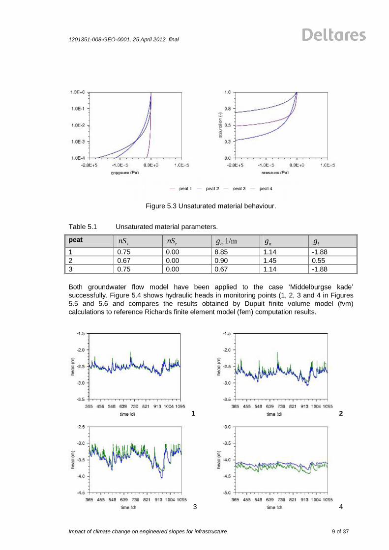
The empirical shape factor lg (-) is often set to 0.5. Tabel 5.1 gathers the imposed unsaturated material behavior for the Richards model for the clusters in the peat dike. The top zone at the canal side (1), the root zone at the polder side (2) and the core of the dike (3). Figure 5.3 presents the unsaturated material behavior graphically.

1201351-008-GEO-0001, 25 April 2012, final


9 of 37

Figure 5.3 Unsaturated material behaviour.

Table 5.1 Unsaturated material parameters.

peat snS rnS ag 1/m ng lg

1 0.75 0.00 8.85 1.14 -1.88 2 0.67 0.00 0.90 1.45 0.55 3 0.75 0.00 0.67 1.14 -1.88 Both groundwater flow model have been applied to the case ‘Middelburgse kade’ successfully. Figure 5.4 shows hydraulic heads in monitoring points (1, 2, 3 and 4 in Figures 5.5 and 5.6 and compares the results obtained by Dupuit finite volume model (fvm) calculations to reference Richards finite element model (fem) computation results.

1 2

3 4


1201351-008-GEO-0001, 25 April 2012, final

10 of 37

Figure 5.4 Hydraulic heads monitoring points.

The finite element mesh used to discretize the Richards' equation included 1526 nodes and 3308 linear elements. A single groundwater flow simulation with 11,000 time steps of 0.1 day took about 2.2 hours on a Intel core2 quad Q6600 2.40 GHz processor. The finite volume mesh was constructed out of three lines of 50 cells each, for which effective parameters were calculated in a preprocessing phase. At the end of a time step groundwater pressures were computed at the nodes of eight lines that correspond to the soil layers in the model using the real material behavior. A simulation over 1,100 time steps of 1.0 day took about 44 seconds on the same computer. The main reason for the large reduction in computational time is due to the linearization of the unsaturated flow process. Figure 5.5 depicts the pressure field for a winter situation calculated by the Richards based model and the phreatic surface that follows from Dupuit computations.

Figure 5.5 Pressure field winter situation (1 December 2005).

Figure 5.6 compares the results for a summer situation. A maximum variation in the position of the water table of one meter was found.

1201351-008-GEO-0001, 25 April 2012, final


11 of 37

Figure 5.6 Pressure field summer situation (19 July 2006).

The results demonstrate a good ability of the Dupuit approximation to simulate groundwater pressure fields. Using Richard's approximation it was found that anisotropy in the permeability tensor due to horizontal layering of peat is very important. The horizontal component of the permeability tensor in the unstructured zone is about ten times its vertical component. This observation justifies the use of the Dupuit approximation for simulating flow through the saturated zone of a peat dike. If preferential flow is taken into account by scaling the permeability then the permeability tensor in the structured zone has a vertical component more than ten times higher than the horizontal component. This generates a dominating vertical inflow through the partly saturated zone, which is captured by the proposed boundary condition that closes the flow problem in the Dupuit model.

1 2


1201351-008-GEO-0001, 25 April 2012, final

12 of 37

3 4

Figure 5.7 Hydraulic heads monitoring points.

Although both groundwater flow models produce results that compare well, it was hard to reproduce observed groundwater heads in monitoring points exactly. A large set of calibration calculations was constructed by which the sensitivity of the output signals for material parameter variations was observed. The position of the monitoring points however showed to be the most sensitive parameter and a better match was found if all the observations were moved 2 meters to the left of their original position. Figure 5.7 compares measured and calculated hydraulic heads in monitoring points in their altered positions. In general the stability of the dike decreases when its weight becomes less and uplift conditions apply. For peat dikes the weight decrease strongly depends on the amount of water that leaves the system by evaporation. Figure 5.8 shows the stability response over the interval under observation and compares the results of the Bishop model with the modified Bishop model, which was presented in chapter 4.

Figure 5.8 Stability response over the measurement interval.

The figures point out a stable situation throughout the simulation period as the stability factor is well above 1.0. The stability factor decreases in the second wet period (around day 730 compare Figure 5.8 for which a shallow slip circle was found. Bishop stability compares well with modified Bishop stability because uplift conditions did not occur and no slip surfaces composed out of circle segments and material interface lines dominated simple circular slip surfaces. A tipping point analysis revealed that an increase of the evapo-transpiration by a

1201351-008-GEO-0001, 25 April 2012, final


13 of 37

factor two leads to failure (stability factor of 1.1) of the peat dike. Figure 5.9 presents the stability response for the evapo-transpiration tipping point analysis.

Figure 5.9 Stability response evapotranspiration tipping point.

The stability factor decreases just after the first dry period and continued to decrease after the second dry period. For these situations, a deep slip circle was found. Bishop stability deviates from modified Bishop stability because uplift conditions occur and composed slip surfaces dominate simple circular slip surfaces.

1201351-008-GEO-0001, 25 April 2012, final


15 of 37

6 Conclusions

The proposed procedure for climate change impact assessment of embankments follows from a dynamic system simulation. Time dependent hydraulic constraints and meteorological conditions provide input signals for the system. The Penmann-Monteith expression generates agro-meteorological boundary conditions for the Dupuit model, which simulates groundwater flow. A modified Bishop expression assesses geo-mechanical stability. Observation wells monitor the geo-hydrologic system behavior and provide data for model calibration. The stability factor response gives a geo-mechanical output signal of the dike system. The main reason for using the Dupuit model instead of the Richards model stems from the fact that the unsaturated material behaviour is often insufficiently known so more advanced calculations can not be supported. Next to this the flow process through the unsaturated zone is very complex due to highly varying meteorological conditions and heterogeneous soil behavior. The proposed model incorporates effective porosity and effective permeability in the unsaturated zone, which can theoretically be based on homogenization of pF-curves. Effective parameters can also be found by a calibration procedure. The effective parameters are found more easily than model parameters that support the pF-curves. The simplified model gives more robust results and is computationally highly efficient. The groundwater flow model has been applied to the case ‘Middelburgse kade’ successfully, although it was hard to obtain observed groundwater heads in monitoring points exactly. Using Richard's model it was found that accounting for anisotropy in the permeability tensor due to horizontal layering of peat is very important. The horizontal component of the permeability tensor in the unstructured zone is about ten times its vertical component. This observation justifies the use of the Dupuit approximation for simulating flow through saturated zone of a peat dike. If preferential flow is taken into account by scaling the permeability then the permeability tensor in the structured zone has a vertical component more than ten times the horizontal component. This generates a dominating vertical inflow through the partly saturated zone, which is captured by the proposed boundary condition that closes the Dupuit model. The water pressure field in a section of the dike under observation was calculated over a period of two years. A maximum variation in the position of the water table of one meter was found. A tipping point analysis revealed that an increase of the evapotranspiration by a factor two leads to failure of the peat dike. To obtain a better understanding in water table conditions of peat dikes under drying and wetting conditions, it is recommended to apply the model to the ‘Stowa’ series of well monitored dikes [4] (Appendix 1). Remote sensing techniques supported by inverse modeling could provide information on the effective porosity and permeability used in the Dupuit model. Real time predictions for the stability of large sections of peat dikes can then be made available and imposing climate scenario's will give a prediction of the impact of climate change for these embankments. Laboratory tests on peat columns support the theoretical basis of the model assumptions; effective parameters can be measured for porosity and permeability and a bulk relation between volumetric change and moisture ratio can be derived. Advanced single-phase (water flow) and multi-phase (water-air flow) calculation will support the findings.

1201351-008-GEO-0001, 25 April 2012, final


17 of 37

Notations

a storage term (-)

ca empirical factor (cm/d) A Angstrom coefficient (-) b slice width (m)

cb soil cover factor (-) B Angstrom coefficient (-) c hydraulic resistance (s)

c cohesion 2(N/m ) ac specific heat capacity (J/kgK) cc crop reflection coefficient (-) rc reflection coefficient (-) sc soil reflection coefficient (-)

vc consolidation coefficient 2(m /s) d aquitard thickness (m) D aquifer thickness (m) e void ratio (-)

ae actual vapor pressure (kPa) ase saturated vapor pressure (kPa)

pE potential evaporation (m/s)

ET evapo-transpiration (m/d) F stability factor (-)

jg gravitational acceleration 2(m/s )

ag Van Genuchten factor (1/m)

lg Van Genuchten factor (-)

mg Mualem's factor (-)

ng Van Genuchten factor (-)

G soil heat flux 2(J/m d) h canopy height (cm) I interception evaporation (m/s) k permeability (m/s)

rk relative permeability (-)

kD transmissivity 2(m /s)

ijK hydraulic conductivity (m/s)

l leave area index (-)


1201351-008-GEO-0001, 25 April 2012, final

18 of 37

n porosity (-)

en effective porosity (-)

in outward pointing normal (-) N relative sunshine duration (-)

p pore pressure 2(N/m ) ap atmospheric pressure (kPa)

P precipitation (m/s) q source term (1/s)

iq specific discharge (m/s)

rq root zone influx (m/s)

sq surface influx (m/s)

iQ discrete influx 2(m /s) r slip circle radius (m)

ar aerodynamic resistance (s/m) cr crop resistance (s/m)

aR extraterrestrial radiation 2(J/m d)

fR resistance force (N) siR short-wave radiation 2(J/m d)

nR net radiation 2(J/m d) lnR net long-wave radiation 2(J/m d) snR net short-wave radiation 2(J/m d)

S saturation (-)

fS loading force (N)

rS minimal saturation (-)

sS maximum saturation (-) t time (s) T average temperature (C)

pT potential transpiration (m/s)

maxT maximum temperature (C)

minT minimum temperature (C) u average wind speed (m/s)

*u wind velocity (m/s)

V bulk volume 3(m )

pV pore volume 3(m )

sV solid phase volume 3(m )

wV water volume 3(m ) w moisture ratio (-)

1201351-008-GEO-0001, 25 April 2012, final


19 of 37

W wet day part (-)

ix Cartesian coordinate (m) z elevation level (m)

hz measurement position (cm)

mz elevation level (cm)

soil compressibility 2(m /N)

c unit conversion (s/d)

water compressibility 2(m /N)

soil unit weight 3(N/m ) a psychometric constant (kPa/K)

domain boundary 1(m ) latitude (deg)

ij intrinsic permeability 2(m )

Lam\a'{e} constants 2(N/m ) w latent vaporization heat (J/kg)

dynamic viscosity 2(kg m/s )

Lam\a'{e} constant 2(N/m )

c vapor pressure slope (kPa/K)

i artificial head (m)

i connectivity (1/s)

fluid density 3(kg/m ) a air density 3(kg/m ) w water density 3(kg/m )

effective stress 2(N/m )

total stress 2(N/m )

shear stress 2(N/m )

f maximum shear stress 2(N/m )

hydraulic head (m) friction angle (deg) pressure head (m)

domain 2(m )

1201351-008-GEO-0001, 25 April 2012, final


21 of 37

References

[1] R.B.J. Brinkgreve, R. Al-Khoury, and J.M. van Esch. Plaxflow. Plaxis B.V., Delft, The Netherlands, 1th edition, 2003.

[2] G. de Marsily. Quantitative Hydrogeology, Groundwater Hydrology for Engineers. Academic Press, 1986.

[3] J.C. van Dam. Field-Scale Water Flow and Solute Transport, SWAP Model Concepts, Parameter Estimation and Case Studies. PhD thesis, Wageningen Universiteit, Wageningen, The Netherlands, 2000.

[4] E. van den Elsen. Eindrapport monitoring waterstanden veenkaden. Alterra, project 231422, december 2006.

[5] J.M. van Esch. Adaptive Multiscale Finite Element Method for Subsurface Flow Simulation. PhD thesis, Delft University of Technology, Delft, The Netherlands, 2010.

[6] J.M. van Esch. Modeling groundwater flow through dikes for real time stability assessment. In Computational Water Resources Research, 2012.

[7] A. Verruijt. Computational Geomechanics, volume 7 of Theory and Applications of Transport in Porous Media. Kluwer Academic Publishers, 1995.

[8] A.H.Weerts, J. Schellekens, and F.S. Weiland. Real-time geospatial data handling and forecasting: Examples from delft-fews forecasting platform/system. Journal of Selected Topics in Applied Earth Observations and Remote Sensing, 2010.

1201351-008-GEO-0001, 25 April 2012, final


23 of 37

Appendix 1 Peat dike series

This appendix presents the ‘Stowa’ series of well monitored dikes [4]. This research program aimed to develop a better understanding in the variation of water table conditions of peat dikes under drying and wetting conditions by monitoring the geo-hydrological behavior of four peat dikes: Middelburgse kade, Brermweg, Kleine Geer and Vierhuis.

VEENGRONDEN

KVro / ZVroGeoxideerd veen

KVoo / ZVooGereduceerd veen

KVrsGeoxideerd kleiig veen

KVooGereduceerd kleiig veen

ZVrsGeoxideerd zandig veen

ZVooGereduceerd zandig veen

LZrsLichte zavel

LKrsZware zavel en lichte klei

ZKrsZware klei

LKooOngerijpte zavel en klei

KooOngerijpte rietklei

MZMatig fijn zand

GZGrof zand

KZKleiig zand

PSPleistoceen zand

KLEIGRONDEN

ZANDGRONDEN

Figure 0.1 Soil types


1201351-008-GEO-0001, 25 April 2012, final

24 of 37

Appendix 1.1 Middelburgse kade

-12.00

-10.00

-8.00

-6.00

-4.00

-2.00

0.000 5 10 15 20 25 30 35

Figure 0.2 Soil profile Middelburgse kade.

-5

-4

-3

-2

-1

00 10 20 30 40

CM2CM1

CM4

Figure 0.3 Groundwater head observation points.

-500

-450

-400

-350

-300

-250

-200

-150

17-fe

b-05

24-fe

b-05

3-m

rt-05

10-m

rt-05

17-m

rt-05

24-m

rt-05

31-m

rt-05

7-ap

r-05

14-a

pr-0

5

21-a

pr-0

5

28-a

pr-0

5

5-m

ei-0

5

12-m

ei-0

5

19-m

ei-0

5

26-m

ei-0

5

2-ju

n-05

9-ju

n-05

16-ju

n-05

23-ju

n-05

30-ju

n-05

7-ju

l-05

14-ju

l-05

21-ju

l-05

28-ju

l-05

4-au

g-05

11-a

ug-0

5

18-a

ug-0

5

25-a

ug-0

5

1-se

p-05

8-se

p-05

15-s

ep-0

5

22-s

ep-0

5

29-s

ep-0

5

6-ok

t-05

13-o

kt-0

5

20-o

kt-0

5

time (days)

grou

ndw

ater

hea

d N

AP [c

m]

M1 Kruin M2 Talud M3 Voet M4 Voet diep Figure 0.4 Observed groundwater heads Middelburgse kade.

1201351-008-GEO-0001, 25 April 2012, final


25 of 37

Appendix 1.2 Bermweg

BERMWEG

-15.00

-13.00

-11.00

-9.00

-7.00

-5.00

-3.00

-1.00 0 5 10 15 20 25 30 35 40

Afstand (m)

hoogte (m NAP)

Figure 0.5 Soil profile Bermweg.

-5.00

-4.00

-3.00

-2.00

-1.00

0.000 10 20 30 40

Afstand (m )

CB2CB1

CB3

Figure 0.6 Groundwater head observation points Bernweg.

-400

-350

-300

-250

-200

-150

-100

28-m

ei-0

5

4-ju

n-05

11-ju

n-05

18-ju

n-05

25-ju

n-05

2-ju

l-05

9-ju

l-05

16-ju

l-05

23-ju

l-05

30-ju

l-05

6-au

g-05

13-a

ug-0

5

20-a

ug-0

5

27-a

ug-0

5

3-se

p-05

10-s

ep-0

5

17-s

ep-0

5

24-s

ep-0

5

1-ok

t-05

8-ok

t-05

15-o

kt-0

5

time (days)

grou

ndw

ater

hea

ds N

AP

[cm

]

B1 Kruin B2 Talud B3 Voet B4 Diepe Voet

Figure 0.7 Observed groundwater heads Bermweg.


1201351-008-GEO-0001, 25 April 2012, final

26 of 37

Appendix 1.3 Kleine Geer

-12.00

-10.00

-8.00

-6.00

-4.00

-2.00

0.000 5 10 15 20 25 30 35

Afstand (m) Figure 0.8 Soil profile Kleine Geer.

-5

-4

-3

-2

-1

00 10 20 30 40

CG2

CG1

CG3

Figure 0.9 Groundwater head observation points Kleine Geer.

-500

-450

-400

-350

-300

-250

-200

-150

-100

-50

0

28-m

ei-0

5

4-ju

n-05

11-ju

n-05

18-ju

n-05

25-ju

n-05

2-ju

l-05

9-ju

l-05

16-ju

l-05

23-ju

l-05

30-ju

l-05

6-au

g-05

13-a

ug-0

5

20-a

ug-0

5

27-a

ug-0

5

3-se

p-05

10-s

ep-0

5

17-s

ep-0

5

24-s

ep-0

5

1-ok

t-05

8-ok

t-05

15-o

kt-0

5

time (days)

grou

ndw

ater

hea

d N

AP

[cm

]

G1 Kruin G2 Talud G3 Voet

Figure 0.10 Observed groundwater heads Kleine Geer.

1201351-008-GEO-0001, 25 April 2012, final


27 of 37

Appendix 1.4 Vierhuis

-6.00

-5.00

-4.00

-3.00

-2.00

-1.00

0.00

1.00

2.00

0 5 10 15 20 25 30 35

Afstand (m)

Steenbestorting

Figure 0.11 Soil profile Vierhuis.

-2

-1

0

1

0 10 20 30 40

CV2CV3

CV1CV4

Figure 0.12 Groundwater head observation points Vierhuis.

time (days)

-200

-150

-100

-50

0

50

100

1-ju

n-05

8-ju

n-05

15-ju

n-05

22-ju

n-05

29-ju

n-05

6-ju

l-05

13-ju

l-05

20-ju

l-05

27-ju

l-05

3-au

g-05

10-a

ug-0

5

17-a

ug-0

5

24-a

ug-0

5

31-a

ug-0

5

7-se

p-05

14-s

ep-0

5

21-s

ep-0

5

28-s

ep-0

5

5-ok

t-05

12-o

kt-0

5

19-o

kt-0

5

grou

ndw

ater

hea

ds N

AP [c

m]

V1 voet V2 talud V3 kruin V4 voet diep

Figure 0.13 Observed groundwater heads Vierhuis.

Date post:	06-Dec-2021
Category:	Documents
Upload:	others
View:	3 times
Download:	0 times

Impact of climate change on engineered slopes for ...

Documents