0

Forthcoming Journal of Investment Management

Impact of Credit Markets on Dynamic Stochastic Real Aggregate Production

by

Thomas S.Y. Ho

President

Thomas Ho Company

New York, NY. USA

And

Sang Bin Lee

Professor of Finance

Hanyang University

Seoul, Korea

April 2014

This paper provides a dynamic stochastic macro-financial model that describes the impact of the

credit market on real production risk and provides some empirical evidence of the

reasonableness of the model. Our model shows that the uncertain real sector output affects the

performance of the credit market, which in turn, impacts the real production of an economy,

resulting in a positive feedback effect. Our model shows that an increase in financial sector

leverage and household sector leverage would induce a stronger feedback effect and increasing

marginal production of financial leverage. Our model identifies the key risk drivers in measuring

the performance of an economy that can be used to attribute quarterly GDP growth rate over the

sample period 2000 Q1 to 2013 Q3. The empirical results can be used to interpret the underlying

causes of economic boom-bust cycles and provide insights into a sustainable GDP growth

pattern.

This macro-finance model has many applications. For example, the risk drivers of the GDP

growth rates can be used to study equity broad-based market returns (Ho and Lee (2014a)).The

model can also be used to specify a structural macro-finance model that can be used to evaluate

efficacy of some financial regulations (Ho and Lee (2014b)).

Keywords: macro-financial models, flow of risk, financial network, GDP growth rate attribution,

financial leverage, household leverage

The authors thank faculty of Owen School of Business, Vanderbilt University, in particular

Miguel Palacios and Hans Stoll for their comments and many conversations related to the paper.

1

Impact of the Credit Market on Dynamic Stochastic Real Aggregate Production

Introduction

Gross Domestic Product (GDP) is arguably the most important measure of economic

performance of an economy. An important approach to analyze stochastic GDP growth rate is to

determine its attribution by specifying the components that constitute its value. Based on the

attributions, market participants can better interpret the underlying economics of the reported

GDP growth rate. Recently, the size of the credit market as an attribute to the uncertainty of

GDP growth rate is of particular importance. From mid-2007 to mid-2013, the US debt market

has grown $30 trillion and the size of China’s shadow banking industry has grown to $7.5

trillion. Financial economists are concerned with the impact of the growth of credit market to the

real output of an economy. Yet, to date, few macro-financial models have empirical relevance

that captures the dynamic stochastic characteristics of the GDP growth rate taking the credit

market into account.

For example, one attribution model is based on the aggregate expenditure constructed on the

accounting identity stating that GDP is the sum of consumption, investment, government

expenditure, and trade imbalance. This accounting identity is static and does not provide us

insights in forecasting or time series estimation. Production functions such as the Cobb-Douglas

function in macroeconomics are used. These production functions assert that the next period

output depends on current capital and labor inputs. These models are dynamic, providing a

model to be estimated using time series, but they pay no attention to uncertainties, which are

considered as “noise”, without modeling the stochastic terms.

Risk structure of GDP growth rate is important in characterizing the performance of an economy.

This is because GDP quarterly growth rates are volatile and such “risk” can only be well-defined

if the market has already established the “expected growth” value. If GDP has grown in the

multiple consecutive cycles, then economists have to decide if the economy has entered a secular

growth cycle with higher expected growth rate or simply some transient positive production

outcome which is called “noise”. Therefore, modeling the risk structure of GDP growth rate and

explaining the temporal changes is necessary to understand the growth rate movements.

2

A growing literature of dynamic stochastic equilibrium models seeks to fill this void. However,

to date, these models typically have not incorporated the role of the financial sector as an integral

part of the economic system and have failed to be empirically relevant.

Using a macro-financial model to specify the risk structure of GDP growth rate can answer the

following questions: Is the financial sector destabilizing economic growth? How do household

leverage and financial leverage affect the stochastic economic growth? Which drivers of

economy provide sustainable secular growth? Which drivers form the components of economic

growth trends? These questions are important to designers of the financial system, financial

regulators, and corporate managers.

We formulate a dynamic stochastic model that describes the impact of real production risk on the

financial sector performance, which in turn, impacts on production. Using the flow of risk

analysis, our model shows that financial leverage and household leverage induce a positive serial

correlation on production. This feedback effect increases (or decreases) in an accelerated rate

with an increase (or decrease) of financial sector and household sector leverages. This non-linear

relationship can be destabilizing to economic growth as market participants tend to increase both

household leverage and financial leverage when the economy grows steadily, and the accelerated

increase in the feedback effect may lead to market fragility.

Intuitively, our model can be explained as follows. We have shown that an economy’s

production based on equity financing, including internal financing, is most important to identify

the performance of an economy. This production output increases the total aggregate asset, and

this additional asset can be used as collateral for credit, funding new projects at a lower cost of

capital by lowering the informational cost of transacting. If the economy can consistently

generate increased equity-financed outputs, then the credit market would provide an additional

positive net present value production. But the converse is also true. In an economic downturn,

the credit market would further add to the loss in production in a “de-leveraging” cycle. We

define this uncertain output from equity funding as production risk. We find both the production

risk and the feedback to have significant explanatory power to the GDP stochastic growth rate.

3

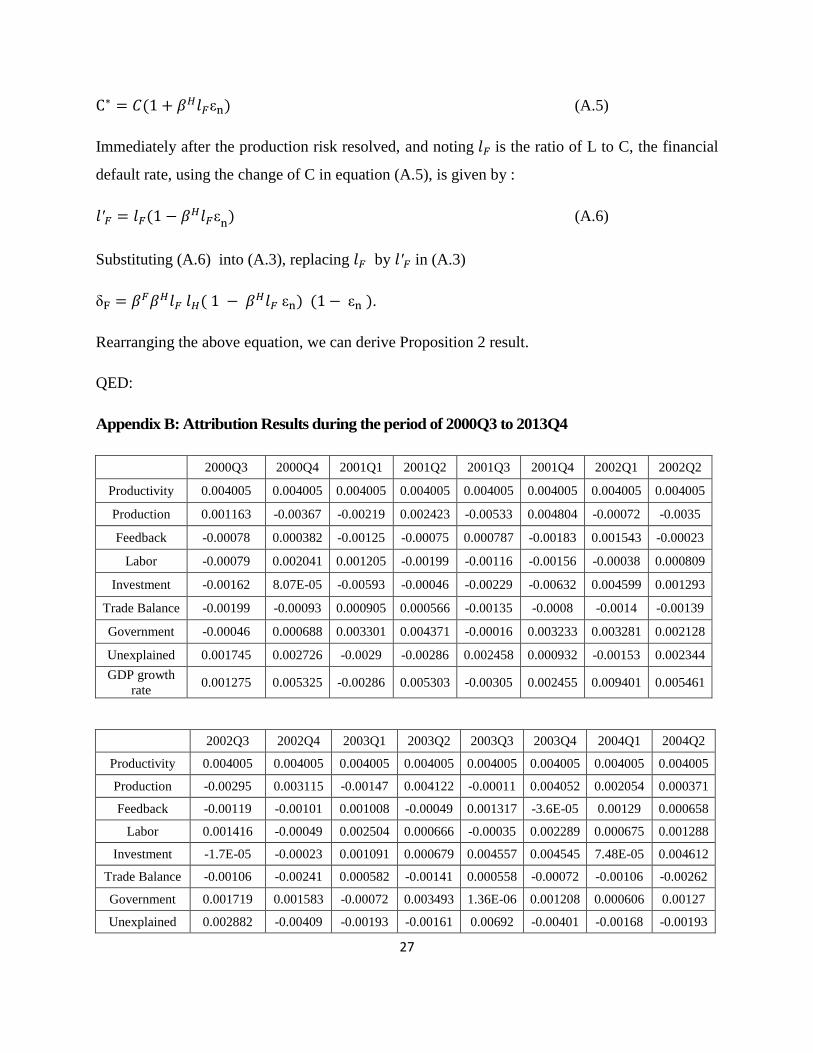
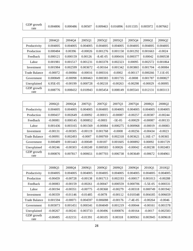
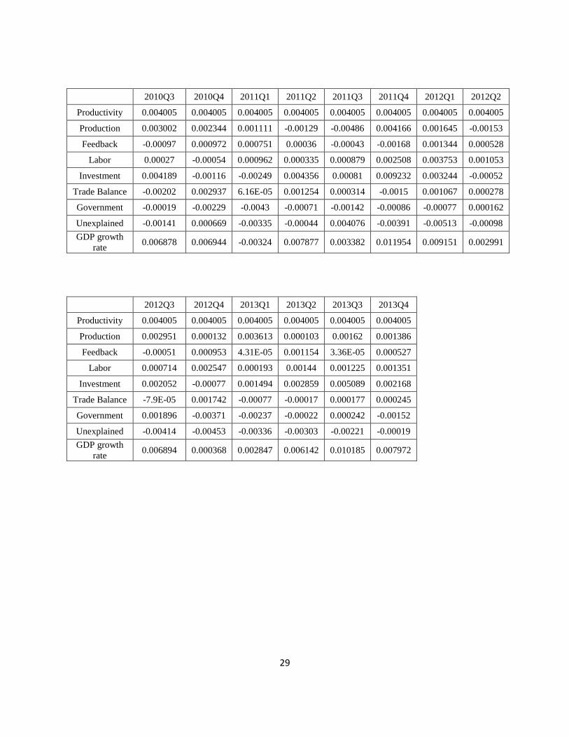
The production risk and the feedback effect enable us to formulate a seven macroeconomic

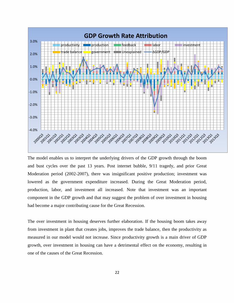
factor stochastic dynamic GDP growth model. The purpose of this empirical study is not to

determine the fundamental factors of the stochastic GDP growth rate as in empirical factor asset

valuation models, but to study how some of the macro-factors may attribute to the changes in the

GDP growth rate. Our empirical evidence tends to support this theoretical model. Our GDP

growth rate attribution results for the sample period from 2000 to 2013 enables us to interpret the

underlying factors that explained the GDP growth through the Great Moderation period (2002-

2007), the Great Recession (2007-2010), and Slow Recovery (2010–2013). The results find that

the production risk and the feedback effect from financial sector are both significant. Their

impact on the boom and bust cycles of the economy provides insights into a measure of a

sustainable GDP growth rate pattern.

Our model differs from macro-finance models that deal with likelihood of sovereign defaults

(Cornelius (2000), Merton and Broglie (2005), Gray et al (2007)). These models analyze the

impact of the credit market on the sovereign default risk by using option such as pricing models.

By way of contrast, our model is not concerned with sovereign defaults but on the impact of the

financial sector on the performance of an economy.

The paper proceeds as follows. There are two main sections in the paper. First, we describe the

real economy as a network tied to the financial sector and use the flow of risk methodology to

formulate the aggregate asset dynamic stochastic model which is then analyzed empirically.

Second, we empirically examine a GDP quarter growth rate attribution model using a Cobb-

Douglas production function framework by extending from our macro-financial model.

Dynamic Stochastic Aggregate Asset Model

This section derives a model of total aggregate asset’s dynamic stochastic process. This paper

extends from the Ho, Palacios, and Stoll, (HPS 2012 and 2013) framework in relating the

financial sector to the real outputs by providing an explicit model of the lagged production risk

structure. For exposition clarity, we summarize HPS model assumptions in this section. HPS

assumes the agents in the economy invest in the aggregate asset for future consumption, with a

4

design of the economy that maximizes real outputs. The productive capacity depends on an

exogenous production risk and the expected net return of the aggregate asset of the economy.

HPS notes that the outstanding credit borrowed must equal to the credit lent in the financial

sector. The agents’ aggregate borrowing is constrained by the size of aggregate real asset used as

collaterals. An increase in the size of the financial sector enhances the allocation of resources

resulting in higher real outputs, which increases the aggregate asset in the economy. This in turn

would lead to a larger financial sector, until the financial sector size is at an optimal level in

balancing an increase in bankruptcy cost.

Technology of the Economy: Aggregate Asset and Production Risk

HPS first considers the real sector without the financial sector. In this case, the dynamics of the

aggregate (real) asset K in the economy depend on a number of factors: the outputs of these

assets, the proportion of this production which is reinvested, and the production shocks on the

economy. The aggregate real asset K evolves over time according to production, investment, and

consumption in the economy. Using a multi-period discrete time model, we assume that the

aggregate real asset K is a linear stochastic process at time t+1:

(1)

where, at time n, is the output per unit of aggregate real asset; c is the combined effect of the

depreciation rate net of investments, and organic growth of the real sector independent of the

financial sector; and the idiosyncratic outputs which we assume to be independent and

identical normal distribution with a constant standard deviation of , where n = 0, 1, ….

This paper deals with the risk of the real sector growth and therefore the production risk is

particularly important in our discussion. Within the context of our model, the production risk is

the uncertain real sector output that results in the change in the aggregate asset value, which

generates future outputs as explained in HPS. This idiosyncratic output, “production risk” ,

requires further explanation. These are idiosyncratic proportional changes of the aggregate real

assets generated by exogenous factors, for example natural and man-made disasters that deplete

real asset value or breakthroughs in technological innovations that enhance real asset value. In

this economy, the household, which includes all agents in the economy including individuals,

5

corporations and government, owns all the aggregate assets and therefore, the household net

worth is also .

In this stylized economy, we do not model the process by which agents in the economy choose to

invest or consume the real assets as it is not essential for understanding the financial system. But

instead we assume that the agents consume and invest in the economy which provides a constant

rate of return . We assume that c is a positive constant, and therefore the value deducted from

the growth of real sector is proportional to the size of the current real sector size.

Institutional Framework of the Economy: Financial System and Market Frictions

HPS assumes that the financial sector consists of financial agreements among the agents of the

economy. For simplicity, the model assumes that the agreements are one-period bonds. To make

implicit an interaction between the real economy and the financial sector, we assume that the

financial sector has the potential of improving the production of real assets, but can also destroy

assets in the case of bankruptcy.

HPS model assumes frictions in the economy with search cost and transaction cost, and

considers a financial system that improves the allocation of real resources and enhances the

performance of the production economy. But these benefits are offset in part by financial

distresses and their associated deadweight loss resulting from bankruptcy costs.

Specifically, we note that the aggregate household asset AH must equal to the total debt

outstanding, the aggregate household liability, L, since every dollar amount borrowed must equal

the amount lent. The aggregate household liability is supported (collateralized) by the aggregate

real asset, K. Therefore, the total asset of the household is sum of the financial asset and the

aggregate real asset, (L + K), and the total liability is L. So, by accounting identity, the net worth

is K. Since the net worth is K, we can define the household leverage to be the ratio of the total

liabilities to net worth:

= L/K (2)

The financial sector can be modeled as an aggregate bank, which HPS calls the Tier 1 financial

system. (Tier 2 incorporates the financial market, an extension that does not affect our

6

conclusions of this paper.) The bank has asset AB, liability L

B, and capital C. By definition of

capital, which is asset net the liability,

AB

= LB + C (3)

But the flow of funds from the household liability to the household asset must pass through this

aggregate bank. And therefore, each household debt (liability) is the bank’s loan (asset). That is:

L = AB (4)

Substituting equation (3) to equation (4), we get:

L = LB + C

Since the household aggregate asset equals the household aggregate liability, we can then

conclude that the aggregate household assets are separated into two classes: capital C and

investments A, which is the aggregate bank’s liability LB. Capital is the total asset net of the total

liabilities of all the financial institutions in the financial system. And therefore,

L = A + C (5)

The bankruptcy cost in the household sector has to pass from the aggregate household liability

side of the household balance sheet to the aggregate household asset side of the balance sheet via

the financial sector. The capital can be viewed as a junior tranche of the aggregate household

asset that absorbs the default costs first. Therefore C is a buffer to credit losses. For this reason,

we can define the financial leverage to be the aggregate bank’s total asset (equaling the

aggregate household liability) to its capital,

= L/C (6)

Flow of Risk: Risk Structure of the Aggregate Asset Stochastic Process

This subsection uses the financial sector framework discussed above and the flow of risk method

to derive the aggregate asset dynamic stochastic process, particularly, its risk structure showing

how the financial leverage, household leverage, and the time series of production risks are

related. The flow of risk describes how the sequence of idiosyncratic outputs flow through the

7

financial system and generate the uncertainties of investments in the aggregate real asset K.

According to equation (1), the risk is measured per unit value, and the risk is a normal

distribution with mean 0 with constant standard deviation of σ.

According to equation (1), the production risk leads to stochastic changes in the aggregate real

asset value K. We assume for the time being that the financial sector size L and the capital C

adjust at the end of each period such that the household leverage and the financial leverage

remain constant at the beginning of each period. The idiosyncratic real output induces

uncertainty to the size of the aggregate real asset, which is collateralizing the household liability.

Therefore, the idiosyncratic outputs induce uncertain bankruptcy cost that flows from the

household sector to the financial sector, and then back to the real sector.

To model this flow of risk, we first assume that the idiosyncratic output is realized at the

beginning of a period. As a result of costly re-contracting in a market with friction, the aggregate

household liability L would remain unchanged for a period. Therefore, the leverages and

would be affected by the change in K. At the end of the period, re-contracting occurs and the

leverages adjust back to and . This lag is important to the model. When there is a failure in

production, our financial capital size and household debt level cannot be adjusted downward

immediately. For example, when the real sector value falls 10%, the debt level does not fall 10%

immediately. The debt level would still be at the ratio to the previous real sector size. The lag

would lead to high debt level for a period and hence higher bankruptcy than it would be.

Therefore, the lag creates a flow of risk of bankruptcy cost from the household liability to

household asset via the financial sector.

The Pathway of the Flow of Risk via Household Sector

The production risk triggers the flow of risk, starting from the household aggregate liabilities,

passing through the financial sector to the household assets, raising or lowering the financial risk

capital of the household sector. The production risk is assumed to affect the credit market size

linearly, proportional to the household leverage. For this paper, we interpret this relationship via

expected bankruptcy cost. The impact of the credit market on the real sector can be also be

8

interpreted in the marginal effect of the credit market on the opportunity of positive net present

value projects.

There are two pathways in the flows of risk. The first pathway starts with the production risk that

triggers household defaults, and the dead weight loss passes to the aggregate real asset. The

second pathway is the dead weight loss that passes from the household liability to the financial

sector, resulting in dead weight loss in the financial sector. And that dead weight loss then passes

from the financial sector to the aggregate real asset K. The first path relates the household

liability to the real sector; the second path relates the household liability and the financial sector

to the real sector. For example, a home owner’s default adds a dead weight loss to the real sector.

Also, the homeowner’s default lowers the aggregate bank’s capital that may trigger financial

institutions’ default. That will also add the dead weight loss to the real economy. The two paths

are described as follows:

For simplicity, we assume that the default rate is proportional to household leverage. We denote

household default rate by . Using the superscript “-“ denotes the value just prior the

realization of the production risk and default events, we have

(7)

Immediately after the realization of the production risk, the real asset value is and

the household leverage becomes

. (8)

By assuming that the standard deviation of is small so that we can ignore the second order

terms, then we have and then the household leverage just before

bankruptcies occur is given by:

(9)

Therefore, equation (7) shows that if the real sector stochastic output is positive, the household

leverage falls, and conversely, if the production stochastic output is negative, the household

leverage would increase.

9

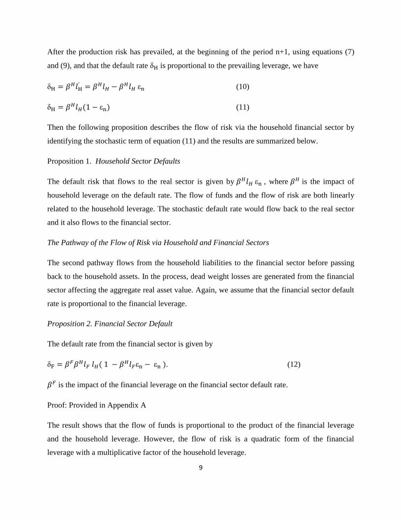
After the production risk has prevailed, at the beginning of the period n+1, using equations (7)

and (9), and that the default rate is proportional to the prevailing leverage, we have

(10)

(11)

Then the following proposition describes the flow of risk via the household financial sector by

identifying the stochastic term of equation (11) and the results are summarized below.

Proposition 1. Household Sector Defaults

The default risk that flows to the real sector is given by , where is the impact of

household leverage on the default rate. The flow of funds and the flow of risk are both linearly

related to the household leverage. The stochastic default rate would flow back to the real sector

and it also flows to the financial sector.

The Pathway of the Flow of Risk via Household and Financial Sectors

The second pathway flows from the household liabilities to the financial sector before passing

back to the household assets. In the process, dead weight losses are generated from the financial

sector affecting the aggregate real asset value. Again, we assume that the financial sector default

rate is proportional to the financial leverage.

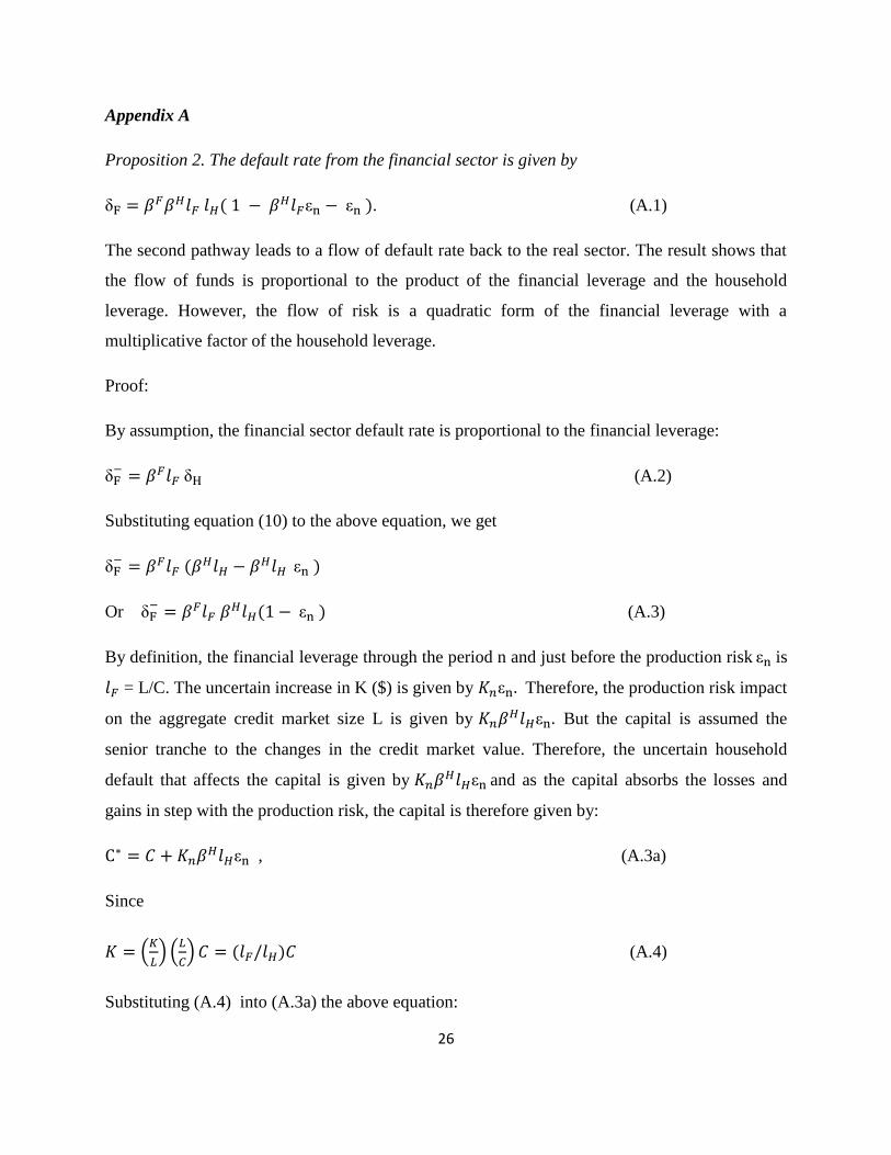
Proposition 2. Financial Sector Default

The default rate from the financial sector is given by

. (12)

is the impact of the financial leverage on the financial sector default rate.

Proof: Provided in Appendix A

The result shows that the flow of funds is proportional to the product of the financial leverage

and the household leverage. However, the flow of risk is a quadratic form of the financial

leverage with a multiplicative factor of the household leverage.

10

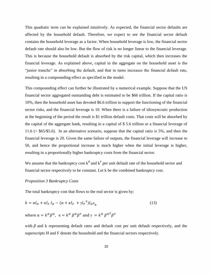
This quadratic term can be explained intuitively. As expected, the financial sector defaults are

affected by the household default. Therefore, we expect to see the financial sector default

contains the household leverage as a factor. When household leverage is low, the financial sector

default rate should also be low. But the flow of risk is no longer linear to the financial leverage.

This is because the household default is absorbed by the risk capital, which then increases the

financial leverage. As explained above, capital in the aggregate on the household asset is the

“junior tranche” in absorbing the default, and that in turns increases the financial default rate,

resulting in a compounding effect as specified in the model.

This compounding effect can further be illustrated by a numerical example. Suppose that the US

financial sector aggregated outstanding debt is estimated to be $66 trillion. If the capital ratio is

10%, then the household asset has devoted $6.6 trillion to support the functioning of the financial

sector risks, and the financial leverage is 10. When there is a failure of idiosyncratic production

at the beginning of the period the result is $1 trillion default costs. That costs will be absorbed by

the capital of the aggregate bank, resulting in a capital of $ 5.6 trillion or a financial leverage of

11.6 (= $65/$5.6). In an alternative scenario, suppose that the capital ratio is 5%, and then the

financial leverage is 20. Given the same failure of outputs, the financial leverage will increase to

50, and hence the proportional increase is much higher when the initial leverage is higher,

resulting in a proportionally higher bankruptcy costs from the financial sector.

We assume that the bankruptcy cost kH

and kF per unit default rate of the household sector and

financial sector respectively to be constant. Let k be the combined bankruptcy cost.

Proposition 3 Bankruptcy Costs

The total bankruptcy cost that flows to the real sector is given by:

(13)

with and k representing default rates and default cost per unit default respectively, and the

superscripts H and F denote the household and the financial sectors respectively.

11

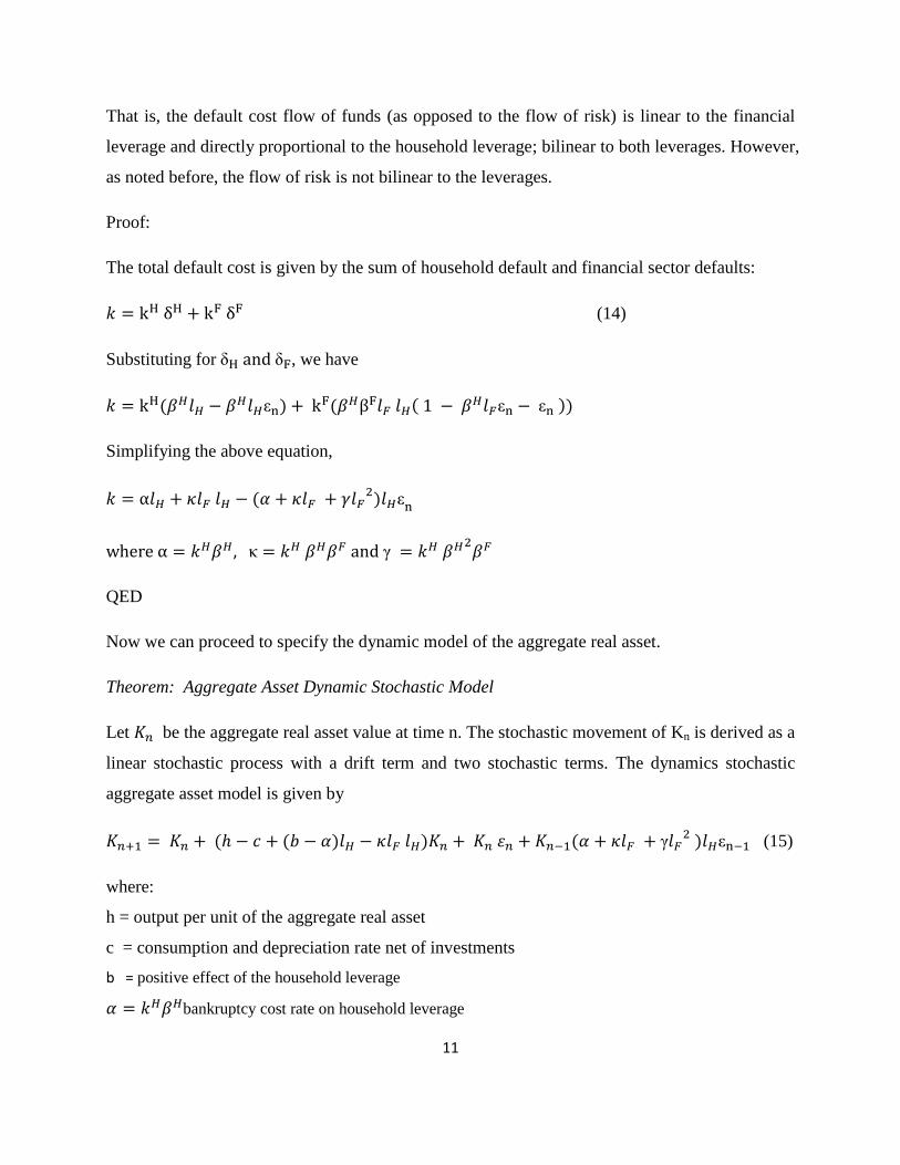
That is, the default cost flow of funds (as opposed to the flow of risk) is linear to the financial

leverage and directly proportional to the household leverage; bilinear to both leverages. However,

as noted before, the flow of risk is not bilinear to the leverages.

Proof:

The total default cost is given by the sum of household default and financial sector defaults:

(14)

Substituting for , we have

Simplifying the above equation,

QED

Now we can proceed to specify the dynamic model of the aggregate real asset.

Theorem: Aggregate Asset Dynamic Stochastic Model

Let be the aggregate real asset value at time n. The stochastic movement of Kn is derived as a

linear stochastic process with a drift term and two stochastic terms. The dynamics stochastic

aggregate asset model is given by

(15)

where:

h = output per unit of the aggregate real asset

c = consumption and depreciation rate net of investments

b = positive effect of the household leverage

bankruptcy cost rate on household leverage

12

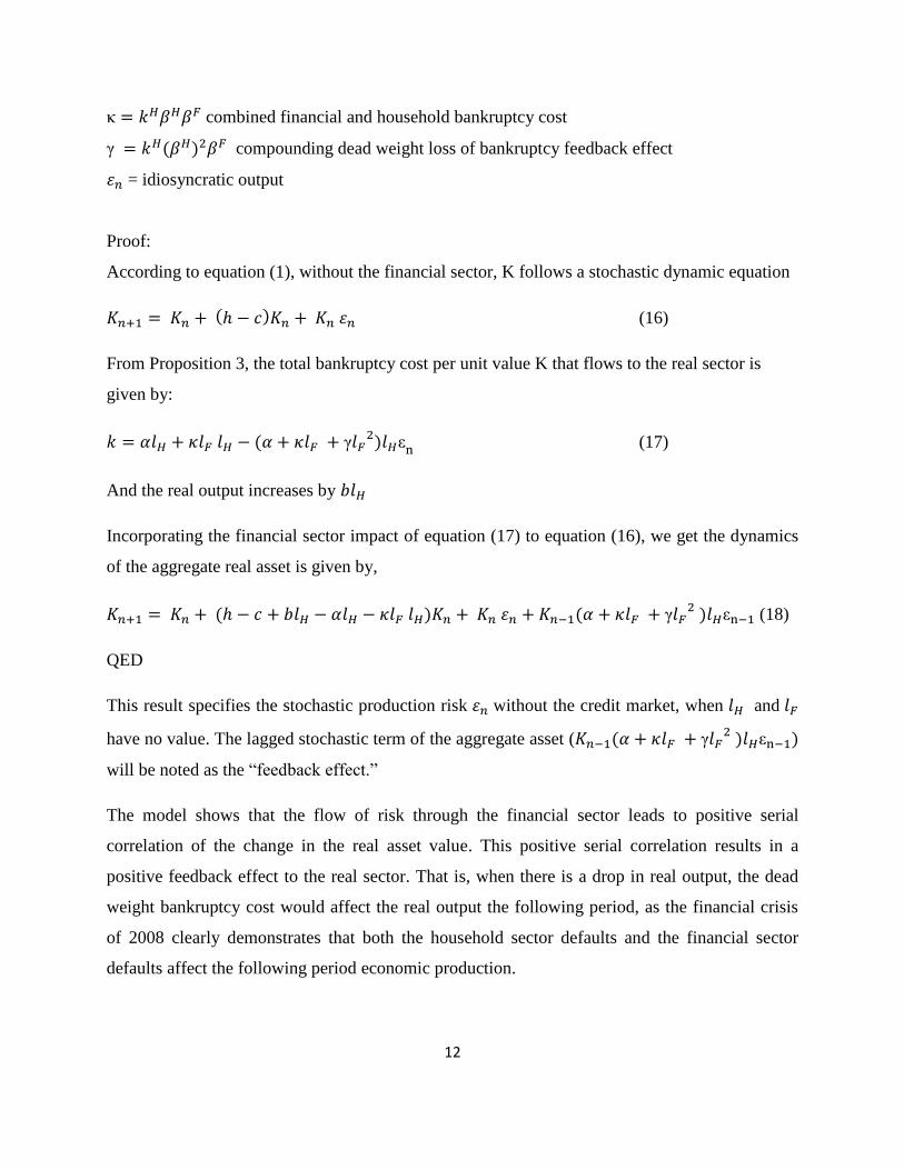
combined financial and household bankruptcy cost

compounding dead weight loss of bankruptcy feedback effect

= idiosyncratic output

Proof:

According to equation (1), without the financial sector, K follows a stochastic dynamic equation

(16)

From Proposition 3, the total bankruptcy cost per unit value K that flows to the real sector is

given by:

(17)

And the real output increases by

Incorporating the financial sector impact of equation (17) to equation (16), we get the dynamics

of the aggregate real asset is given by,

(18)

QED

This result specifies the stochastic production risk without the credit market, when and

have no value. The lagged stochastic term of the aggregate asset (

will be noted as the “feedback effect.”

The model shows that the flow of risk through the financial sector leads to positive serial

correlation of the change in the real asset value. This positive serial correlation results in a

positive feedback effect to the real sector. That is, when there is a drop in real output, the dead

weight bankruptcy cost would affect the real output the following period, as the financial crisis

of 2008 clearly demonstrates that both the household sector defaults and the financial sector

defaults affect the following period economic production.

13

Note that default risk is induced by the idiosyncratic outputs. When the real output production

exceeds market’s expectation, the default rate would also fall. The feedback effect should also be

observed when the economy outperforms expectation.

This result has direct implications to macro risk management as it shows that an increase in the

credit market can enhance the productivity of the economy, but at the same time, induces a

higher volatility of the aggregate real asset value, resulting in higher production risk. And

therefore, macro risk management has to balance these two effects on the real output in

managing the size of the credit market.

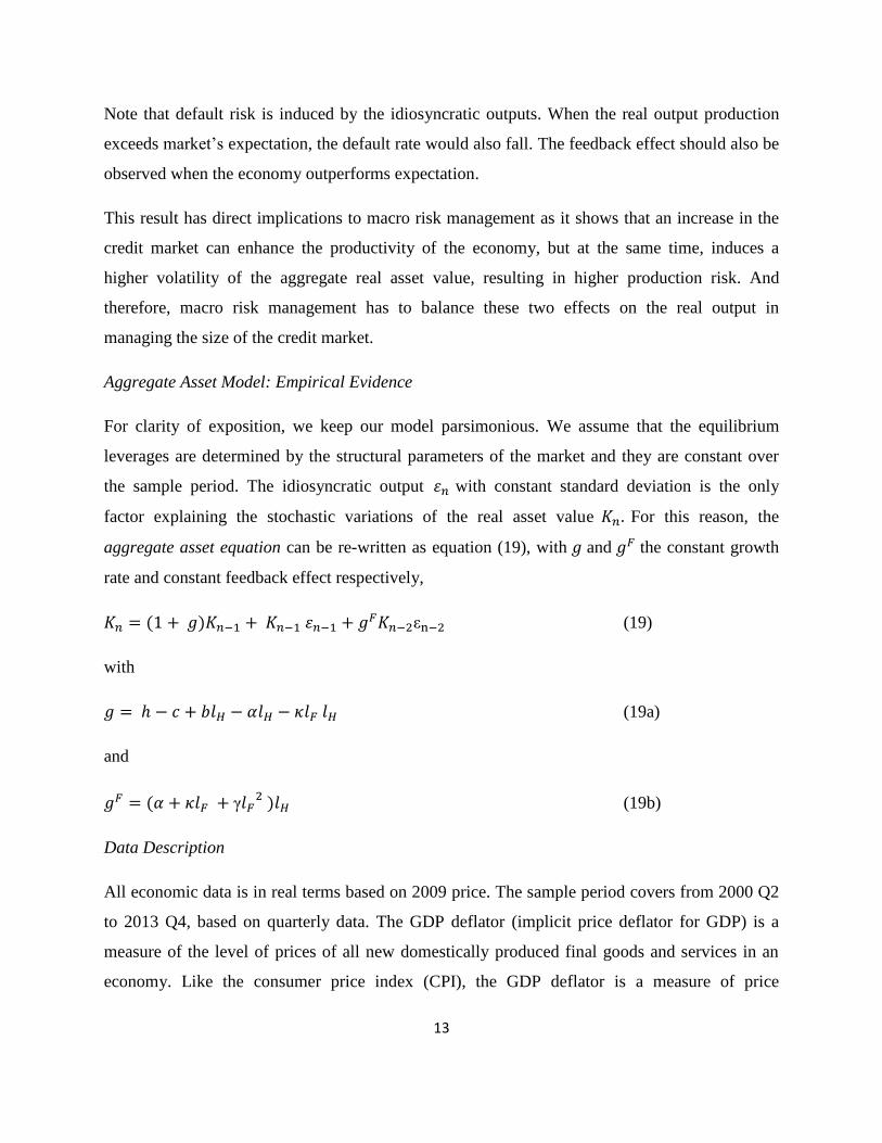
Aggregate Asset Model: Empirical Evidence

For clarity of exposition, we keep our model parsimonious. We assume that the equilibrium

leverages are determined by the structural parameters of the market and they are constant over

the sample period. The idiosyncratic output with constant standard deviation is the only

factor explaining the stochastic variations of the real asset value For this reason, the

aggregate asset equation can be re-written as equation (19), with and the constant growth

rate and constant feedback effect respectively,

(19)

with

(19a)

and

(19b)

Data Description

All economic data is in real terms based on 2009 price. The sample period covers from 2000 Q2

to 2013 Q4, based on quarterly data. The GDP deflator (implicit price deflator for GDP) is a

measure of the level of prices of all new domestically produced final goods and services in an

economy. Like the consumer price index (CPI), the GDP deflator is a measure of price

14

inflation/deflation with respect to a specific base year; the GDP deflator of the base year itself

2009 is equal to 100. The quarterly time series of the GDP are obtained from the Federal Reserve

Board.

We use the household net worth as proxy to the aggregate real asset. Household net worth is the

sum of the market value of assets owned by every member of the household minus liabilities

owed by household members. Wealth in the United States is commonly measured in term of this

household net worth. Here we use only household net worth rather than the sum of the corporate

net worth and the household net worth to avoid the double counting. The labor data comes from

the quarterly civilian employment from US Department of Labor. The household net worth,

investment, export, import, and the government expenditure data are collected from St. Louis

Federal bank.

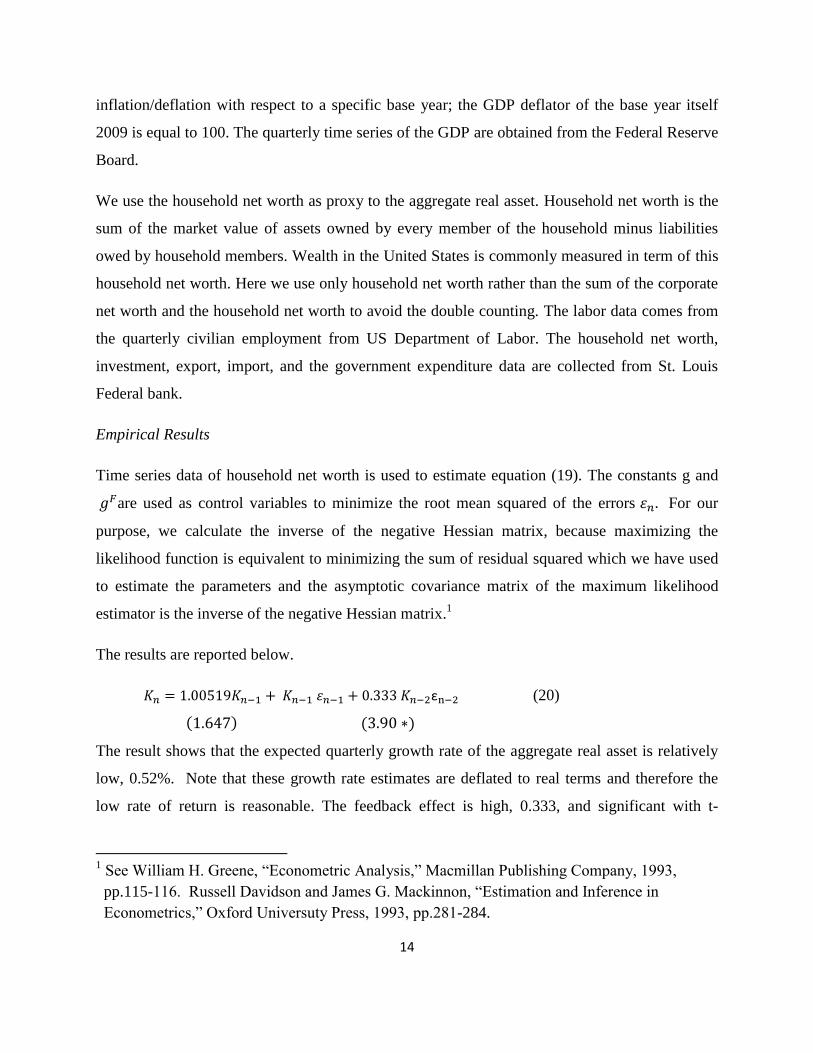
Empirical Results

Time series data of household net worth is used to estimate equation (19). The constants g and

are used as control variables to minimize the root mean squared of the errors For our

purpose, we calculate the inverse of the negative Hessian matrix, because maximizing the

likelihood function is equivalent to minimizing the sum of residual squared which we have used

to estimate the parameters and the asymptotic covariance matrix of the maximum likelihood

estimator is the inverse of the negative Hessian matrix.1

The results are reported below.

(20)

The result shows that the expected quarterly growth rate of the aggregate real asset is relatively

low, 0.52%. Note that these growth rate estimates are deflated to real terms and therefore the

low rate of return is reasonable. The feedback effect is high, 0.333, and significant with t-

1 See William H. Greene, “Econometric Analysis,” Macmillan Publishing Company, 1993,

pp.115-116. Russell Davidson and James G. Mackinnon, “Estimation and Inference in

Econometrics,” Oxford Universuty Press, 1993, pp.281-284.

15

statistics of 3.90. The results show that approximately a third of the idiosyncratic product output

is fed back to the real economy the following period, since is close to 1.

The standard deviation of the quarterly production risk ( ) is 2.47% or annualized 4.95%. The

standard deviation of the proportional change of is 2.68%, or annualized 5.35%. This result

shows that risk of aggregate asset value is magnified by the feedback effect, with an increase of

0.4%, in comparing the standard deviation of the aggregate real asset to that of the production

risk.

Discussion

This feedback effect is important in the literature in discussing financial fragility. C.

Kindleberger (1978) describes how a financial crisis is triggered by a default event that would

lead to a fall in prices across the market as agents adjust their expectations of returns, and that in

turn would create business failures. Allen and Gale (1998) argues the low asset returns would

lead to banks unable to meet their obligations, resulting in fire sale of asset, depressing asset

prices further. The feedback effect can also be observed when an economy is growing. Hyman

Minsky (1986) argues that when the economy is growing, risk premium would tighten, resulting

in higher leverage ratio, which in turns leads to economic expansion. This feedback effect results

in further tightening of the risk premium and raising the leverage ratios. Dalio (2013) provides a

detail explanation of the feedback effect. He describes the mechanics of leveraging and de-

leveraging of an economy based on monetary policy, resulting in changes in real outputs.

Ho, Palacios, and Stoll (2013) describes the financial leverage and household leverage would

both increase when the economy expands reaching a partial equilibrium. Ho and Lee (2014 b)

extends HPS model to derive those optimal household and financial leverage levels. Our model

provides a model to this feedback effect that has been discussed in this literature.

The contribution of our estimate of the feedback effect based on our model has two folds: (1) we

have quantified the feedback effect, which is shown to be significant; (2) we have shown that

observed change in aggregate asset is, in a significant way, an accumulation of changes of the

aggregate of previous cycles and not just the innovation of the current cycle. Therefore, our

results show that the change in the aggregate asset value per se does not update only new

16

information, only portion of the value change is current information. The aggregate asset value

dynamic stochastic process is not martingale. Therefore the results suggest that we should isolate

the real production factor from feedback effect to determine trends of economic growth.

GDP Growth Rate Attribution

The previous section shows that the credit market induces a positive feedback effect to the

change in aggregate asset. This section uses this result to extend a parsimonious empirical GDP

growth rate model, which is then used to specify an attribution model of GDP growth. The

purpose of this empirical model is provide a relatively simple tool to analyze reported growth

rate of GDP, enabling us to identify some of the attributes of the GDP growth rate in the boom

and bust cycles, such as the role of government expenditure, employment rate, and other

attributes that may relate to the underlying causes of economic cycles.

A GDP Growth Rate Model

We assume that the real asset K can be measured by the household net worth. Consistent with

macro equilibrium models, the economic output can be viewed as a constant rate of return of the

aggregate real asset, as discussed in HPS (2012, 2013). This model assumes labor to be held

constant as input to the GDP. To incorporate labor input into the production function, we use a

dynamic form of a Cobb-Douglas function. That is, we consider the following real output

equation of the real output GDP, denoted by :

(21)

L denotes the civilian employment in the economy. and are elasticities of the aggregate asset

and labor to the production respectively. is the residual term. Equation (21) assumes that the

economy is closed and that all outputs are consumed immediately such that outputs and

expenditure are reported in the same period. These assumptions lead to estimation error of .

This error term can be explained by the expenditure side of the real output identity. In particular,

we assume that

(22)

17

where G, I and T are the real government consumption expenditure and gross investment, the

real gross private domestic investment and the difference between real export and real import of

goods and services (trade balance) respectively.

Since these independent variables are constructed to explain the residual of equation (21), they

are constructed with no expected values with the time-series data de-trended. The purpose of

equation (22) is not to identify how much these components can explain the GDP growth rate.

The purpose of the estimate is to identify the factors not explained by the production function.

Note that we have not considered using consumption as an explanatory variable in equation (22)

because our test has shown that the consumption independent variable has little explanatory

power, even though consumption is an important component of GDP.

The system of equations (19), (21) and (22) provides us an empirically relevant model whereby

each equation can be estimated. Linear regressions are applied and the results are provided below.

Estimation results for equation (21),

+

(23)

(4.68*) (3.95*) (3.02*)

The adjusted is 37.64

Equation (22) seeks to determine the factors that can explain the residuals of equation (23), based

on the expenditure perspective of the GDP measure. Estimation of equation (21),

+ (24)

(5.61*) (10.72*) (-4.49*)

The adjusted is 68.24

Risk Contribution by Attributes

18

The results can be re-written as a model of the quarterly changes of GDP. We substitute equation

(20) to equations (23) and (24), then the GDP growth rate growth rate model can be described

below

(25)

Each term of equation (25) is called an “attribute” of the GDP growth rate. Equation (25) shows

that the GDP quarter growth rate is the sum of the constant term A0 and risk attributes denoted by

Ai ( i = 1, 2,…,7). And the Attribution Equation is given below:

= ∑ Ai for i = 0,…, 7. (26)

Each attribute is described as follows: Productivity ( This attribute is derived from

productivity (a) and the growth rate of the household net worth (g), which has estimated to be

almost negligible. For this reason, intuitively, we think of the intercept to be productivity in the

Cobb-Douglas function sense. Production Risk (0.11042 ): This attribute is an important

determinant of the GDP growth rate uncertainty, since the production risk attribute is the risk

driver of the real outputs of the economy. Feedback Effect (0.03663 ): This

attribute should be as important as the production risk by comparing the magnitude of the

coefficients for the production risk and the feedback attributes. This result is consistent with the

view that the reported GDP reflects not just the current outputs but also the outputs of previous

periods; and this lagged effect is induced by the credit market. Labor Attribute (

This attribute is derived from the employed labor, which has minimal growth over the sample

period. Equation (25) shows that the significant demographic effect on the GDP growth rate.

Government Attribute This attribute derived from the observed government

expenditure that has not been explained by the production function. The result to be discussed

later shows that counter-cyclical action of the government expenditure to the performance of the

real outputs. Investment Attribute (

This attribute is derived from the observed

investment expenditure. The investment attribute is an important component of the GDP. Trade

balance Attribute (

This attribute is derived from the observed trade imbalance.

19

Since the US is not export-oriented country compared to Japan, this attribute is relatively small.

Unexplained Attribute : This is the idiosyncratic term unexplained by the model.

We first study the correlations of the seven risk attributes, where the correlation matrix is

denoted by . The results are provided below

Production Feedback Labor Investment Trade Government Unexplained

Production 1.00 0.05 0.17 0.31 -0.10 -0.07 -0.42

Feedback 0.05 1.00 0.44 0.50 -0.13 -0.36 -0.04

Labor 0.17 0.44 1.00 0.51 -0.30 -0.25 -0.25

Investment 0.31 0.50 0.51 1.00 -0.50 -0.24 -0.09

Trade -0.10 -0.13 -0.30 -0.50 1.00 0.07 -0.01

Government -0.07 -0.36 -0.25 -0.24 0.07 1.00 0.08

Unexplained -0.42 -0.04 -0.25 -0.09 -0.01 0.08 1.00

The results can be explained intuitively. Trade imbalance and government expenditure tend to be

anti-cyclical to the production. On the other hand, labor and investment are positively related to

the production. Interestingly, investment is strongly correlated to the feedback effect, suggesting

that investment level depends on the production of the previous cycle. Investment decisions are

affected by the observed production as well as the projected future production. Investment is

related strongly to labor, as one might expect.

We can now determine the risk contribution of each risk attribute to the volatility of the GDP

quarterly growth rates. Let be the ith attribute’s standard deviation estimated over the sample

period. Since the attributions’ variations explain the variations of the GDP growth rates, the

following equation must hold:

(27)

In re-arranging, we get

(28)

Let (29)

20

and

Ci = / (30)

Then we have derived the following risk contribution equation

i =1 (31)

where Ci is interpreted as the contribution of risk by the ith attribute. That is, we can decompose

the standard deviation of the GDP growth rate into seven components, Ci . The

quarterly GDP growth rate standard deviation decomposition (%) is presented in the table below.

Descriptions Production Feedback Labor Investment

Trade balance Government Unexplained

Standard

Deviation (%)

0.273 0.092 0.204 0.458 0.188 0.212 0.259

Contribution

(%)

20.993 58.898

Note the value βi adjusts for the correlations of the attributes. For example, if one attribute is

negatively correlated with another, then the contributions of these two attributes would be

lowered when their combined effect is considered. This measure of βi is applied to calculate

cross hedging strategies in investment literature in determining imperfect hedging strategies. The

application of this methodology is the same for our purpose here.

The results show that the significant contributors are the investment (57%), production risk (21%)

and labor (17.63%). The results can be explained intuitively. The quarterly standard deviation of

investment is significant. 0.44% adds to the GDP growth on one standard deviation probability.

Furthermore, investment is strongly positively correlated to the feedback and labor attributions

while the production does not have such positive correlation. Since GDP growth rate are driven

by these attributes, investment becomes an important explanatory factor in the GDP growth

uncertainty. Likewise the unexplained attribute is relatively small (3.66%) even though its

standard deviation is not negligible. That is because the unexplained parameter has minimal

correlations with other attributes. Also, both government expenditure and trade have negative

21

contribution to risk because they tend to be counter-cyclical, providing a “hedge” to the risk of

economic growth rate. The result suggests that investment and production risk together explains

almost 80% of GDP growth rate variations and are important to identify GDP growth trends.

GDP Quarterly Growth Rate Attribution Analysis

This risk contribution result can be extended further to study the inter-temporal behavior of these

attributes using equation (25). We can determine the attributes of the growth rate every quarter

over the sample period. The attribution results are presented below graphically. The numerical

results are presented in Appendix B. The sample period spans from 2000 to 2013, quarterly

observations. The blue line is the quarterly growth rate in GDP. The bar chart depicts the

attributions to the GDP growth rate for each quarter. For example, in the case of 2nd

quarter in

2006, the growth rate of GDP from the 1st quarter in 2006 is 0.3113%, to which the productivity

contributes 0.4005%; production contributes -0.2402%; feedback effect contributes 0.0538%;

labor contributes 0.1864%; investment contributes -0.1293%; trade balance contributes 0.0141;

government contributes 0.0286% and unexplained contributes -0.0032%. The sum of the

contribution is equal to the GDP growth rate.

22

The model enables us to interpret the underlying drivers of the GDP growth through the boom

and bust cycles over the past 13 years. Post internet bubble, 9/11 tragedy, and prior Great

Moderation period (2002-2007), there was insignificant positive production; investment was

lowered as the government expenditure increased. During the Great Moderation period,

production, labor, and investment all increased. Note that investment was an important

component in the GDP growth and that may suggest the problem of over investment in housing

had become a major contributing cause for the Great Recession.

The over investment in housing deserves further elaboration. If the housing boom takes away

from investment in plant that creates jobs, improves the trade balance, then the productivity as

measured in our model would not increase. Since productivity growth is a main driver of GDP

growth, over investment in housing can have a detrimental effect on the economy, resulting in

one of the causes of the Great Recession.

-4.0%

-3.0%

-2.0%

-1.0%

0.0%

1.0%

2.0%

3.0% GDP Growth Rate Attribution

productivity production feedback labor investment

trade balance government Unexplained ΔGDP/GDP

23

The first downturn of production is in Q2 2006, four cycles ahead of the Great Recession. The

Great Recession (2007-2010) saw all the attributes fall, except for trade and government

expenditure to support that market. Slow Recovery (2010 – 2013) period has two phases. For the

first six cycles, global economy was going through the Euro-crisis. The recovery was led by

investments and not production. Starting from Q4 2011, the results show that the production

remained positive in consecutive cycles, similar in pattern to that of the Great Moderation period.

Ideally, the GDP growth should be stable, with no excess investment or government expenditure

impact. In terms of the attribution graph, such sustainable GDP growth would be depicted with

fairly positive constant production. Hence feedback attributes with also a positive labor attribute.

If this growth can be realized over a stretch a time period, then these changes would be captured

by the productivity attribute. That is, the economy would grow by a significant accumulation of

total aggregate asset and with a higher production efficiency (an increase of productivity). The

GDP growth rate attribution for 2013 Q1, Q2, Q3 , as depicted in the figure, seem to be

consistent with this description, but of course, such consistency over three quarters does not

imply that the US economy is actually on a sustainable growth path. (When the GDP growth is

expected to stable, the returns of the stock market should also capture such an expectation. Ho

and Lee (2014a) also shows that the S&P index returns were consistent with this view over that

period).

The results also show that the US economy on average grows only 1.6% annually over past 13

years and nearly all that growth comes from increase in productivity (as interpreted from the

production function) and not from the higher outputs generated by increase aggregate asset. The

results also suggest that production attribute is most important in driving real output growth, as a

consistent positive production attribute would lead to stable growth path. Trade imbalance and

government expenditure are just counter-cyclical. Investment itself may lead to over-investment.

The intent of this paper is not to analyze the historical GDP growth rate in detail. Applying the

attribution model to study the production of an economy, such as studies of over-investment,

demographic shifts, is beyond the scope of the paper. In this section, we just want to illustrate

24

how the attribution model can provide insight into the risk drivers of the stochastic behavior of

the GDP growth rate. Further discussion will be left for future research.

Summary and Conclusions

Extending Ho, Palacios, and Stoll (2012, 2013) framework, this paper first presents a macro-

financial model, which we then use to formulate a GDP growth rate attribution model. We also

provide some empirical results that may suggest that the model can provide insights into the real

sector performance.

Our macro-financial model shows that the financial sector influences a positive feedback to the

real output. This paper uses a flow of risk methodology to determine the structure of this

feedback effect and we show that the stochastic GDP growth rate has a lagged term, the feedback

effect. And this lagged term depends on the household leverage and financial leverage in a non-

linear way. This feedback effect can be destabilizing to economic growth as market participants

tend to increase both household leverage and financial leverage when the economy grows

steadily. Higher in the leverages result in stronger feedback effects.

The GDP attribution model has eight economic factors. The factors are: productivity, production

risk, feedback effect, labor, government expenditure, trade imbalance, investment, and residuals.

We propose that the most important attribute to sustain stable economic growth is productivity.

The production factor is most important to identify the performance of an economy.

We use the attribution model to study the GDP quarterly growth rate from 2000Q1 to 2013Q3.

The empirical results of the attribution show that the model has reasonable explanatory power

with only 1.8% of the historical GDP quarterly growth rate variations unexplained. The

production and feedback effects account for 29% of the variation.

The attribution results also present the sources of the real output risks over the sample period of

13 years. The results show that during the Great Moderation period, much of the GDP growth

came from increases in investment and labor, without significant increase in production. In fact,

25

the production attribute turned negative in 2006, several cycles ahead of the beginning of the

Great Recession. The result also shows that the first three cycles of 2013 seem to follow a more

stable growth path. These results suggest that the attribution model may be able to provide useful

insight into the performance of the economy.

This paper has many usable applications. The model can be applied to investment. Ho and Lee

(2014 a) show that broad based indices’ returns do not depend on the GDP growth rate per se but

on the risk derivers of the GDP growth rate, taking the feedback effect of the credit market into

account. Since market fragility may result from “irrational exuberance” of unjustified

expectation of economic performance, it is important to tie prospective analysis (equity market

valuation) and retrospective analysis (equity return attribution) in a coherent framework. Today,

return attribution is an important risk management tool. The return attribution of broad-based

equity indices enables analysis of market returns.

Our model can also be applied to evaluate efficacy of financial regulations. Ho and Lee (2014 b)

extends this model to a structural macro-finance model, endogenizing the optimal household

leverage and financial leverage to study the appropriate level of risk capital that should be

embedded in an economic network system. Our model results provide an important component

to a macrostructure theory that describes the dynamic and stochastic relationships of real output,

financial sector and regulations (Ho and Lee (2014c).

26

Appendix A

Proposition 2. The default rate from the financial sector is given by

. (A.1)

The second pathway leads to a flow of default rate back to the real sector. The result shows that

the flow of funds is proportional to the product of the financial leverage and the household

leverage. However, the flow of risk is a quadratic form of the financial leverage with a

multiplicative factor of the household leverage.

Proof:

By assumption, the financial sector default rate is proportional to the financial leverage:

(A.2)

Substituting equation (10) to the above equation, we get

Or

(A.3)

By definition, the financial leverage through the period n and just before the production risk is

= L/C. The uncertain increase in K ($) is given by Therefore, the production risk impact

on the aggregate credit market size L is given by But the capital is assumed the

senior tranche to the changes in the credit market value. Therefore, the uncertain household

default that affects the capital is given by and as the capital absorbs the losses and

gains in step with the production risk, the capital is therefore given by:

, (A.3a)

Since

(A.4)

Substituting (A.4) into (A.3a) the above equation:

27

(A.5)

Immediately after the production risk resolved, and noting is the ratio of L to C, the financial

default rate, using the change of C in equation (A.5), is given by :

(A.6)

Substituting (A.6) into (A.3), replacing by in (A.3)

.

Rearranging the above equation, we can derive Proposition 2 result.

QED:

Appendix B: Attribution Results during the period of 2000Q3 to 2013Q4

2000Q3 2000Q4 2001Q1 2001Q2 2001Q3 2001Q4 2002Q1 2002Q2

Productivity 0.004005 0.004005 0.004005 0.004005 0.004005 0.004005 0.004005 0.004005

Production 0.001163 -0.00367 -0.00219 0.002423 -0.00533 0.004804 -0.00072 -0.0035

Feedback -0.00078 0.000382 -0.00125 -0.00075 0.000787 -0.00183 0.001543 -0.00023

Labor -0.00079 0.002041 0.001205 -0.00199 -0.00116 -0.00156 -0.00038 0.000809

Investment -0.00162 8.07E-05 -0.00593 -0.00046 -0.00229 -0.00632 0.004599 0.001293

Trade Balance -0.00199 -0.00093 0.000905 0.000566 -0.00135 -0.0008 -0.0014 -0.00139

Government -0.00046 0.000688 0.003301 0.004371 -0.00016 0.003233 0.003281 0.002128

Unexplained 0.001745 0.002726 -0.0029 -0.00286 0.002458 0.000932 -0.00153 0.002344

GDP growth

rate 0.001275 0.005325 -0.00286 0.005303 -0.00305 0.002455 0.009401 0.005461

2002Q3 2002Q4 2003Q1 2003Q2 2003Q3 2003Q4 2004Q1 2004Q2

Productivity 0.004005 0.004005 0.004005 0.004005 0.004005 0.004005 0.004005 0.004005

Production -0.00295 0.003115 -0.00147 0.004122 -0.00011 0.004052 0.002054 0.000371

Feedback -0.00119 -0.00101 0.001008 -0.00049 0.001317 -3.6E-05 0.00129 0.000658

Labor 0.001416 -0.00049 0.002504 0.000666 -0.00035 0.002289 0.000675 0.001288

Investment -1.7E-05 -0.00023 0.001091 0.000679 0.004557 0.004545 7.48E-05 0.004612

Trade Balance -0.00106 -0.00241 0.000582 -0.00141 0.000558 -0.00072 -0.00106 -0.00262

Government 0.001719 0.001583 -0.00072 0.003493 1.36E-06 0.001208 0.000606 0.00127

Unexplained 0.002882 -0.00409 -0.00193 -0.00161 0.00692 -0.00401 -0.00168 -0.00193

28

GDP growth

rate 0.004806 0.000486 0.00507 0.009463 0.016896 0.011335 0.005972 0.007662

2004Q3 2004Q4 2005Q1 2005Q2 2005Q3 2005Q4 2006Q1 2006Q2

Productivity 0.004005 0.004005 0.004005 0.004005 0.004005 0.004005 0.004005 0.004005

Production 0.000484 0.00396 -0.00026 0.001276 0.001158 0.001292 0.001663 -0.0024

Feedback 0.000121 0.000159 0.00126 -8.4E-05 0.000416 0.000377 0.00042 0.000538

Labor 0.001981 0.001517 0.001231 0.003378 0.002323 0.00095 0.002572 0.001864

Investment 0.001984 0.002599 0.003672 -0.00164 0.001342 0.003865 0.001704 -0.00084

Trade Balance -0.00072 -0.00084 -0.00016 0.000316 -0.0002 -0.00117 0.000266 7.11E-05

Government 0.000849 -0.00098 0.000463 0.000383 0.001735 -0.0008 0.001787 0.000827

Unexplained 6.95E-05 -0.00199 0.000728 -0.00218 -0.00263 -0.00298 -0.00029 -0.00095

GDP growth

rate 0.008776 0.008432 0.010943 0.005454 0.008149 0.005541 0.012131 0.003113

2006Q3 2006Q4 2007Q1 2007Q2 2007Q3 2007Q4 2008Q1 2008Q2

Productivity 0.004005 0.004005 0.004005 0.004005 0.004005 0.004005 0.004005 0.004005

Production 0.000437 0.002649 -0.00092 -0.00015 -0.00087 -0.00257 -0.00387 -0.00244

Feedback -0.00081 0.000145 0.000852 -0.0003 -5E-05 -0.00029 -0.00087 -0.00133

Labor 0.001436 0.003165 0.001569 -0.00084 0.000275 0.000968 -0.00019 -0.00083

Investment -0.00131 -0.00305 -0.00119 0.001768 -0.0008 -0.00256 -0.00434 -0.0023

Trade Balance -0.00091 0.002493 -0.0007 0.000769 0.002318 0.003621 1.16E-17 0.00365

Government 0.000489 0.001443 -0.00049 0.00187 0.001605 0.000892 0.00092 0.001729

Unexplained -0.00246 -0.00303 -0.00249 0.000583 0.00026 -0.00042 -0.00238 0.002483

GDP growth

rate 0.000876 0.007817 0.000651 0.007703 0.006738 0.003649 -0.00672 0.004961

2008Q3 2008Q4 2009Q1 2009Q2 2009Q3 2009Q4 2010Q1 2010Q2

Productivity 0.004005 0.004005 0.004005 0.004005 0.004005 0.004005 0.004005 0.004005

Production -0.00459 -0.00728 -0.00138 0.001713 0.002193 -0.00017 0.001013 -0.00288

Feedback -0.00083 -0.00159 -0.00261 -0.00047 0.000559 0.000706 -5.5E-05 0.000331

Labor -0.00194 -0.00351 -0.00775 -0.00368 -0.00279 -0.00318 0.000749 0.001942

Investment -0.00359 -0.01146 -0.01485 -0.0078 -0.00112 0.010348 0.004185 0.006659

Trade Balance 0.001594 -0.00071 0.004597 0.006088 -0.00176 -7.4E-05 -0.00264 -0.0046

Government 0.003073 0.001451 0.000341 0.004049 0.001219 -0.00044 -0.00161 0.001578

Unexplained -0.00267 -0.00241 0.003733 -0.00496 0.000876 -0.00164 -0.0017 0.002583

GDP growth

rate -0.00495 -0.02151 -0.01391 -0.00105 0.00318 0.009561 0.003945 0.009618

29

2010Q3 2010Q4 2011Q1 2011Q2 2011Q3 2011Q4 2012Q1 2012Q2

Productivity 0.004005 0.004005 0.004005 0.004005 0.004005 0.004005 0.004005 0.004005

Production 0.003002 0.002344 0.001111 -0.00129 -0.00486 0.004166 0.001645 -0.00153

Feedback -0.00097 0.000972 0.000751 0.00036 -0.00043 -0.00168 0.001344 0.000528

Labor 0.00027 -0.00054 0.000962 0.000335 0.000879 0.002508 0.003753 0.001053

Investment 0.004189 -0.00116 -0.00249 0.004356 0.00081 0.009232 0.003244 -0.00052

Trade Balance -0.00202 0.002937 6.16E-05 0.001254 0.000314 -0.0015 0.001067 0.000278

Government -0.00019 -0.00229 -0.0043 -0.00071 -0.00142 -0.00086 -0.00077 0.000162

Unexplained -0.00141 0.000669 -0.00335 -0.00044 0.004076 -0.00391 -0.00513 -0.00098

GDP growth

rate 0.006878 0.006944 -0.00324 0.007877 0.003382 0.011954 0.009151 0.002991

2012Q3 2012Q4 2013Q1 2013Q2 2013Q3 2013Q4

Productivity 0.004005 0.004005 0.004005 0.004005 0.004005 0.004005

Production 0.002951 0.000132 0.003613 0.000103 0.00162 0.001386

Feedback -0.00051 0.000953 4.31E-05 0.001154 3.36E-05 0.000527

Labor 0.000714 0.002547 0.000193 0.00144 0.001225 0.001351

Investment 0.002052 -0.00077 0.001494 0.002859 0.005089 0.002168

Trade Balance -7.9E-05 0.001742 -0.00077 -0.00017 0.000177 0.000245

Government 0.001896 -0.00371 -0.00237 -0.00022 0.000242 -0.00152

Unexplained -0.00414 -0.00453 -0.00336 -0.00303 -0.00221 -0.00019

GDP growth

rate 0.006894 0.000368 0.002847 0.006142 0.010185 0.007972

30

References

Cornelius, Peter K, 2000. “Trade in Financial Services, Capital Flows, and the Value-at-Risk of

Countries” research notes in economics & statistics, No. 00-2

Dalio, Ray “Forget Econ 101. Take a look at the lessons in Dalio 101” 2013

Gray, Dale, Robert C. Merton, and Zvi Bodie. 2007 “New Framework for Measuring and

Managing Macro-Financial Risk and Financial Stability” NBER working paper

Ho, Thomas and Sang Bin Lee “Stock Indices’ Macro-Based Factor Models and Indices’ Return

Attributions” Working Paper 2014b a

Ho, Thomas and Sang Bin Lee “Structural Macro-Financial Model and Risk Management”

Working Paper 2014b

Ho, Thomas and Sang Bin Lee, “Real Output, Financial System and Regulations: a

Macrostructure Theory” Working Paper 2014c

Ho, Thomas, Miguel Palacios, and Hans Stoll, “Dynamic Financial System: Complexity,

Fragility and Regulatory Principles” Financial Markets, Institutions and Instruments, New York

University, 2013

Ho, Thomas, Miguel Palacios, and Hans Stoll, “Regulatory Principles for the Financial System,”

the Journal of Derivatives, Fall 2012.

Kindleberger, Charles Panic and Crashes A History of Financial Crisis (basic book 1978) 107-108

Merton, R. and Z. Bodie. 2005. “Design of Financial Systems: Toward a Synthesis of Function

and Structure.” Journal of Investment Management 3:1:1–23.

Minsky, Hyman Stabilizing an Unstable Economy (New Haven, Conn Yale University Press

1986) 173