Page 1
Impact of distributed generation on
distribution system
By
Angel Fernández Sarabia
Department of Energy Technology
A Dissertation Submitted to
the Faculty of Engineering, Science and Medicine, Aalborg University
in Partial Fulfilment for the Degree of
Master Graduate
June 2011
Aalborg, Denmark
Page 2
2
Aalborg University
Department of Energy Technology
Pontoppidanstraede 101
9220 Aalborg East, Denmark
Printed in Denmark by Aalborg University
Page 3
3
Title: Impact of Distributed Generation on Distribution System
Semester: 10th
Semester theme: EPSH 4
Project period: Spring - 2011
ECTS: 30
Supervisor: Pukar Mahat
Project group: 1001
__________________________________
Angel Fernández Sarabia
Copies: 2
Pages, total: 107
Appendix: 1
By signing this document, each member of the group confirms that all participated
in the project work and thereby that all members are collectively liable for the
content of the report.
SYNOPSIS: As the yearly electric energy
demand grows, there is a significant increase
in the penetration of distributed generation
(DG) to fulfil this increase in demand.
Integration of a DG into an existing
distribution system has many impacts on the
system, with the power system protection
being one of the major issues. Short circuit
power of a distribution system changes when
its state changes. Short circuit power also
changes when some of the generators in the
distribution system are disconnected. This
may result in elongation of fault clearing
time and hence disconnection of equipments
in the distribution system or unnecessary
operation of protective devices. In this thesis,
the effect of DG penetration on the short
circuit level has been analyzed in a
distribution system with wind turbine and
gas turbine generators. Different cases have
been studied. Location and technology of the
DG sources are changed to study the effect
that these changes may have on the
coordination of protective directional over-
current relays.
Page 5
5
To my family and friends
Page 6
6
Acknowledgement
I would like to express my deep gratitude and appreciation to my supervisor
Assistant Professor Pukar Mahat for his suggestions, patience and encouragement
throughout the period of this work. His support, understanding and expertise have been
very important in completing this research.
I want to take this opportunity to thank my parents and family for their love, constant
support and their precious advice through my life.
Page 7
7
Abstract
As the yearly electric energy demand grows, there is a significant increase in the
penetration of distributed generation (DG) to fulfil this increase in demand.
Interconnecting DG to an existing distribution system provides various benefits to
several entities as for example the owner, utility and the final user. DG provides an
enhanced power quality, higher reliability of the distribution system and can peak
shaves and fill valleys. However, the integration of DG into existing networks has
associated several technical, economical and regulatory questions. Penetration of a DG
into an existing distribution system has many impacts on the system, with the power
system protection being one of the major issues. DG causes the system to lose its radial
power flow, besides the increased fault level of the system caused by the
interconnection of the DG. Short circuit power of a distribution system changes when
its state changes. Short circuit power also changes when some of the generators in the
distribution system are disconnected. This may result in elongation of fault clearing
time and hence disconnection of equipments in the distribution system or unnecessary
operation of protective devices. Therefore, new protection schemes for both DG and
utility distribution networks have been developed in the recent years but the issue has
not been properly addressed. In this thesis, the effect of DG penetration on the short
circuit level has been analyzed in a distribution system with wind turbine and gas
turbine generators. Different cases have been studied. Location and technology of the
DG sources are changed to study the effect that these changes may have on the
coordination of protective directional over-current relays (DOCR). Results are
compared to that of the normal case to investigate the impact of the DG on the short
circuit currents flowing through different branches of the network to deduce the effect
on protective devices and some conclusions are documented.
Page 8
8
Table of contents
Acknowledgment ..…………………………………………………….. 6
Abstract ..………………………………………………………………. 7
Chapter 1
Introduction ..…………………………………………………………. 11
1.1 Traditional Concept of Power Systems ..……………………………. 11
1.2 New Concept of Power Systems ..……………………………………. 12
1.3 Distributed Generation ………………………………………………. 13
1.4 Problem Statement …………………………………………………… 14
1.5 Thesis Objectives ……………………………………………………... 15
1.6 Scope and Limitations ………………………………………………. 15
1.7 Outline of the Thesis …………………………………………………. 17
Chapter 2
Literature Review ……………………………………………………. 18
2.1 Introduction ………………………………………………………….. 18
2.2 Types of Distributed Generation ……………………………………. 19
2.2.1 Photovoltaic Systems ………………………………………………………. . 19
2.2.2 Wind Turbines ………………………………………………….. 20
2.2.3 Fuel Cells …………………………………………………………………….. 21
2.2.4 Micro-Turbines ……………………………………………………………… 21
Page 9
9
2.2.5 Induction and Synchronous Generators……………………………………. 22
2.3 Impact of Distributed Generation on Power System Grids ………. 24
2.3.1 Impact of DG on Voltage Regulation………………………………………. 24
2.3.2 Impact of DG on Losses ……………………………………………………. 26
2.3.3 Impact of DG on Harmonics ……………………………………………… 27
2.3.4 Impact of DG on Short Circuit Levels of the Network …………………. .. 29
2.4 Protection Coordination ……………………………………………………. 31
2.5 Islanding of a Power Network ……………………………………………… 33
2.5.1 Intentional Islanding ……………………………………………………. … 35
2.5.2 Islanding Detection …………………………………………………………. 35
2.6 Impact of DG on Feeder Protection ……………………………………….. 37
2.6.1 Mal-Trip and Fail to Trip …………………………………………………. 38
2.6.2 Reduction of Reach of Protective Devices ………………………………… 39
2.6.3 Failure of Fuse Saving Due to Loss of Recloser-Fuse Coordination …… . 40
Chapter 3
Over-current Protection of Distributed Systems ………………………… 45
3.1 Introduction ……………………………………………………………………… 45
3.2 Types of Over-current Relays ………………………………………………. 45
3.2.1 Definite Current Relay …………………………………………………….… 45
3.2.2 Definite Time Relay ……………………………………………………. …. 46
3.2.3 Inverse Time Relay ……………………………………………………. …… 47
3.3 Model of an Over-current Relay ………………………………………….... 48
Page 10
10
3.4 Directional Over-current Relay Protection Coordination …………. 49
3.4.1 Relay Protection Coordination of Radial Systems ………………………… 50
3.4.2 Relay Protection Coordination with Distributed Generation …………… 51
Chapter 4
Modelling and Simulation Results …………………………………………….. 59
4.1 Modelling of Distribution System …………………………………………. 59
4.2 Design of Over-current Relays for the Test Distribution
System ……………………………………………………. …………………………….. 61
4.3 Modelling of Modified Distribution System ……………………………… 71
4.4 Design of Over-current Relays for the Modified Test
Distribution System …………………...………………………………………………. 72
4.5 Solutions for Issues with Protection in Presence of a
Significant Number of DG………………………..……………………………... 87
4.5.1 Distance Relays ……………………………………………………. ……….. 87
4.5.2 Differential Relays …………………………………………………………... 88
4.5.3 Adaptive Protection ……………………………………………………. …… 90
Chapter 5
Conclusion ……………………………………………………………………………... 92
5.1 Summary and Conclusion ……………………………………………………. 92
5.2 Future Work ……………………………………………………………………. 93
Reference …………………………………………………………………………….…. 95
Appendix ……………………………………………………………………………….. 99
Page 11
Chapter1: Introduction
11
Chapter 1
Introduction
1.1 Traditional Concept of Power Systems
Currently, most of the power systems generate and supplies electricity having into
account the following considerations [1],[2]:
Electricity generation is produced in large power plants, usually located close to
the primary energy source (for instance: coil mines) and far away from the
consumer centres.
Electricity is delivered to the customers using a large passive distribution
infrastructure, which involves high voltage (HV), medium voltage (MV) and
low voltage (LV) networks.
These distribution networks are designed to operate radially. The power flows
only in one direction: from upper voltage levels down-to customers situated
along the radial feeders.
In this process, there are three stages to be passed through before the power
reaching the final user, i.e. generation, transmission and distribution.
GENERATION
TRANSMISSION
DISTRIBUTION
CUSTOMERS
LEVEL 1
LEVEL 2
LEVEL 3
LEVEL 4
ENERGY
FLOW
Fig. 1.1 Traditional industrial conception of the electrical energy supply
Page 12
Chapter1: Introduction
12
In the first stage the electricity is generated in large generation plants, located in non-
populated areas away from loads to get round with the economics of size and
environmental issues. Second stage is accomplished with the support of various
equipments such transformers, overhead transmission lines and underground cables.
The last stage is the distribution, the link between the utility system and the end
customers. This stage is the most important part of the power system, as the final power
quality depends on its reliability [2].
The electricity demand is increasing continuously. Consequently, electricity
generation must increase in order to meet the demand requirements. Traditional power
systems face this growth, installing new support systems in level 1 (see figure 1.1).
Whilst, addition in the transmission and distribution levels are less frequent.
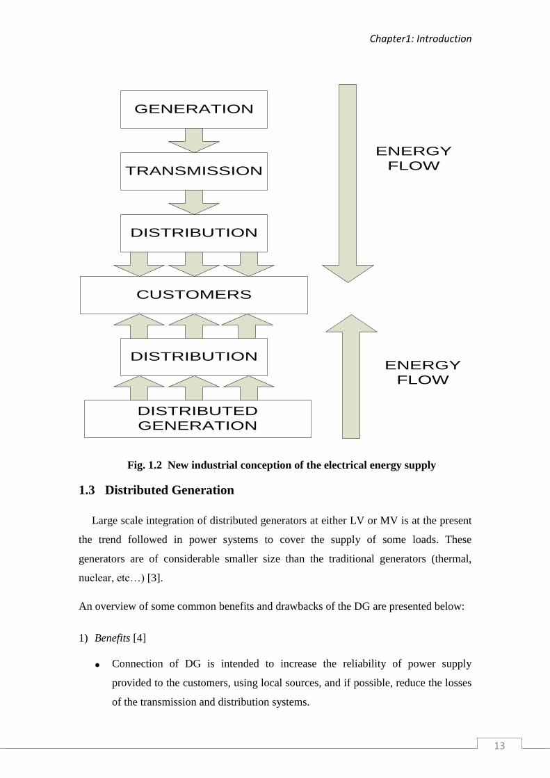
1.2 New Concept of Power Systems
Nowadays, the technological evolution, environmental policies, and also the
expansion of the finance and electrical markets, are promoting new conditions in the
sector of the electricity generation [2].
New technologies allow the electricity to be generated in small sized plants.
Moreover, the increasing use of renewable sources in order to reduce the environmental
impact of power generation leads to the development and application of new electrical
energy supply schemes.
In this new conception, the generation is not exclusive to level 1. Hence some of the
energy-demand is supplied by the centralized generation and another part is produced
by distributed generation. The electricity is going to be produced closer to the
customers.
Page 13
Chapter1: Introduction
13
GENERATION
TRANSMISSION
DISTRIBUTION
CUSTOMERS
ENERGY
FLOW
DISTRIBUTION
DISTRIBUTED
GENERATION
ENERGY
FLOW
Fig. 1.2 New industrial conception of the electrical energy supply
1.3 Distributed Generation
Large scale integration of distributed generators at either LV or MV is at the present
the trend followed in power systems to cover the supply of some loads. These
generators are of considerable smaller size than the traditional generators (thermal,
nuclear, etc…) [3].
An overview of some common benefits and drawbacks of the DG are presented below:
1) Benefits [4]
Connection of DG is intended to increase the reliability of power supply
provided to the customers, using local sources, and if possible, reduce the losses
of the transmission and distribution systems.
Page 14
Chapter1: Introduction
14
The connection of DG to the power system could improve the voltage profile,
power quality and support voltage stability. Therefore, the system can withstand
higher loading situations.
The installation of DG takes less time and payback period. Many countries are
subsidizing the development of renewable energy projects through a portfolio
obligation and green power certificates. This incentives investment in small
generation plants.
Some DG technologies have low pollution and good overall efficiencies like
combined heat and power (CHP) and micro-turbines. Besides, renewable energy
based DG like photovoltaic and wind turbines contribute to the reduction of
greenhouse gases.
2) Drawbacks [4]
Many DG are connected to the grid via power converters, which injects
harmonics into the system.
The connection of DG might cause over-voltage, fluctuation and unbalance of
the system voltage if coordination with the utility supply is not properly
achieved.
Depending on the network configuration, the penetration level and the nature of
the DG technology, the power injection of DG may increase the power losses in
the distribution system.
Short circuit levels are changed when a DG is connected to the network.
Therefore, relay settings should be changed and if there is a disconnection of
DG, relay should be changed back to its previous state.
1.4 Problem Statement
Nowadays, the power electricity demand is growing fast and one of the main tasks
for power engineers is to generate electricity from renewable energy sources to
overcome this increase in the energy consumption and at the same time reduce
environmental impact of power generation. The use of renewable sources of energy has
Page 15
Chapter1: Introduction
15
reached greater importance as it promotes sustainable living and with some exceptions
(biomass combustion) does not contaminant. Renewable sources can be used in either
small-scale applications away from the large sized generation plants or in large-scale
applications in locations where the resource is abundant and large conversion systems
are used [5].
Nevertheless, problems arise when the new generation is integrated with the power
distribution network, as the traditional distribution systems have been designed to
operate radially, without considering the integration of the this new generation in the
future. In radial systems, the power flows from upper terminal voltage levels down to
customers situated along the radial feeders [4].Therefore, over-current protection in
radial systems is quite straightforward as the fault current can only flow in one direction.
With the increase of penetration of DG, distribution networks are becoming similar to
transmission networks where generation and load nodes are mixed (“mesh” system) and
more complex protection design is needed. In this new configuration, design
considerations regarding the number, size location and technology of the DG connected
must be taken into account as the short circuit levels are affected and miss coordination
problems with protection devices may arise [7], [8].
This research addresses some of the issues encountered when designing the over-
current protection coordination between protection devices, in case that a number of DG
sources are connected to a radial system.
1.5 Thesis Objectives
The main objective of this thesis is to investigate the impact that different
configurations and penetration levels of DG may have on the protection of
distribution systems.
The second objective is to develop possible solutions for issues with protection
in presence of a significant number of DG.
1.6 Scope and Limitations
The scope and limitations of this research are as follows:
Only the major technical issues with over-current protection coordination of a
distribution system are covered.
Page 16
Chapter1: Introduction
16
The DG technologies have been limited to gas turbine generators (GTG), which
are based on synchronous generators and fixed speed wind turbines (WTG),
which are based on induction generators.
In case of combined heat and power plants, which consists of gas turbines, heat
generation is not considered. The electricity is considered as the main output of
the plant.
Models have been developed in DIgSILENT/Power Factory and many of the
standard models available in DIgSILENT have been used.
1.7 Outline of the Thesis
This thesis contains 5 chapters and one appendix. It is organized as follows:
Chapter 1: Introduction
This chapter gives a brief introduction to the concept of distributed generation
reflecting the importance of DG systems to both the utility network and customers,
besides the drawbacks occurring if DG is connected to the distribution systems.
Chapter 2: Literature Review
This chapter is divided into six sections: the first section is a brief introduction and a
definition of DG, followed by the second section which discusses the various types of
distributed generation technologies and their nature. The impacts of DG on power
system grids are discussed in the third section. Section four high lights one of the most
important issues to maintain a safe operation of the DG, the protection coordination.
Section five is an overview of one of the major problems, islanding, that miss-protection
can lead to and causes difficulties in system restoration. Finally the last section
discusses the impact of DG penetration on the distribution feeder protection and the
miss-protection problems arising from the interconnection of DGs.
Chapter 3: Over-current Protection of Distributed Systems
This chapter is divided in four sections: the first section gives a brief introduction to
over-current protection technique and some examples of protection devices used in
Page 17
Chapter1: Introduction
17
distribution systems. The second section describes the types of over-current relays and
some of their main features. Section three explains the model of the over-current relay
created in DIgSILENT used throughout this thesis. Finally, in section four a practical
application example using a small test distribution system and the proposed relay model
is given. Some simulations are carried out using the test system and the main problems
encountered in protection coordination of relays, both with and without distributed
generation installed in the system are shown.
Chapter 4: Modelling and Simulation results
In this chapter, simulations results with different DG configurations are presented.
The chapter is divided into five sections: the first section describes the modelling of the
distribution system. In the second section, design of the over-current relay protection is
explained, illustrating two main cases: firstly in Case 1, the test system is analyzed
without the presence of DG, it is the base case that results are compared to. Then, in
Case 2, the test network topology is modified introducing DG at different locations, as
well as, changing the DG technology, showing the effect on the level of short circuit
currents. In the section three, it is described the modelling of the modified distribution
system. Section four, describes the design of the over-current relays protection for this
modified system, several case are analyzed for different levels of penetration of DG. A
small discussion on the results is made at the end of each case and some conclusions are
drawn. The last section presents, some solutions that may be implemented to overcome
the issues found with over-current protection of distributed system.
Chapter 5: Conclusion
Some conclusions are presented in this chapter. The chapter ends naming some of the
works that can be done in the future with reference to the work presented in this
research.
Appendix
It presents data for test systems, generators, excitation system and speed governor.
Page 18
Chapter2: Literature Review
18
Chapter 2
Literature Review
2.1 Introduction
Distributed Generation (DG) is one of the new trends in power systems used to
support the increased energy-demand. There is not a common accepted definition of
DG as the concept involves many technologies and applications. Different countries use
different notations like “embedded generation”, “dispersed generation” or
“decentralized generation”.
Furthermore, there are variations in the definition proposed by different
organizations (IEEE, CIGRE…) that may cause confusion. Therefore in this thesis, the
following definition is used [8]:
Distributed generation is considered as an electrical source connected to the power
system, in a point very close to/or at consumer´s site, which is small enough compared
with the centralized power plants.
To clarify about the DG concept, some categories that define the size of the
generation unit are presented in Table 2.1.
Table 2.1
Size of the DG [10]
Type Size
Micro distributed generation 1Watt < 5kW
Small distributed generation 5kW < 5 MW
Medium distributed generation 5 MW < 50MW
Large distributed generation 50MW < 300MW
The different DG technologies and impacts of distributed generation are introduced
in this chapter; besides, islanded operation and the impact of DG on distribution feeder
protection are presented.
Page 19
Chapter2: Literature Review
19
2.2 Types of Distributed Generation
DG can be classified into two major groups, inverter based DG and rotating machine
DG. Normally, inverters are used in DG systems after the generation process, as the
generated voltage may be in DC or AC form, but it is required to be changed to the
nominal voltage and frequency. Therefore, it has to be converted first to DC and then
back to AC with the nominal parameters through the rectifier [10].
In this chapter, some of the DG technologies, which are available at the present:
photovoltaic systems, wind turbines, fuel cells, micro turbines, synchronous and
induction generators are introduced.
2.2.1 Photovoltaic Systems
A photovoltaic system, converts the light received from the sun into electric energy.
In this system, semiconductive materials are used in the construction of solar cells,
which transform the self contained energy of photons into electricity, when they are
exposed to sun light. The cells are placed in an array that is either fixed or moving to
keep tracking the sun in order to generate the maximum power [9].
These systems are environmental friendly without any kind of emission, easy to use,
with simple designs and it does not require any other fuel than solar light. On the other
hand, they need large spaces and the initial cost is high.
In Fig. 2.1, a photovoltaic panel is shown.
Fig. 2.1 Schematic diagram of a photovoltaic system [11]
Page 20
Chapter2: Literature Review
20
PV systems generate DC voltage then transferred to AC with the aid of inverters.
There are two general designs that are typically used: with and without battery storages.
2.2.2 Wind Turbines
Wind turbines transform wind energy into electricity. The wind is a highly variable
source, which cannot be stored, thus, it must be handled according to this characteristic.
A general scheme of a wind turbine is shown in Fig. 2.2, where its main components are
presented [9].
Fig. 2.2 Schematic operation diagram of a wind turbine [12]
The principle of operation of a wind turbine is characterized by two conversion steps.
First the rotor extract the kinetic energy of the wind, changing it into mechanical torque
in the shaft; and in the second step the generation system converts this torque into
electricity.
In the most common system, the generator system gives an AC output voltage that is
dependent on the wind speed. As wind speed is variable, the voltage generated has to be
transferred to DC and back again to AC with the aid of inverters. However, fixed speed
wind turbines are directly connected to grid [9].
Page 21
Chapter2: Literature Review
21
2.2.3 Fuel Cells
Fuel cells operation is similar to a battery that is continuously charged with a fuel gas
with high hydrogen content; this is the charge of the fuel cell together with air, which
supplies the required oxygen for the chemical reaction [9].
The fuel cell utilizes the reaction of hydrogen and oxygen with the aid of an ion
conducting electrolyte to produce an induced DC voltage. The DC voltage is converted
into AC voltage using inverters and then is delivered to the grid.
In Fig. 2.3 the operation characteristics of a fuel cell are presented.
Fig. 2.3 Schematic diagram of a fuel cell [13]
A fuel cell also produces heat and water along with electricity but it has a high
running cost, which is its major disadvantage. The main advantage of a fuel cell is that
there are no moving parts, which increase the reliability of this technology and no noise
is generated. Moreover, they can be operated with a width spectrum of fossil fuels with
higher efficiency than any other generation device. On the other hand, it is necessary to
assess the impact of the pollution emissions and ageing of the electrolyte characteristics,
as well as its effect in the efficiency and life time of the cell [10].
2.2.4 Micro-Turbines
A micro-turbine is a mechanism that uses the flow of a gas, to covert thermal energy
into mechanical energy. The combustible (usually gas) is mixed in the combustor
chamber with air, which is pumped by the compressor. This product makes the turbine
Page 22
Chapter2: Literature Review
22
to rotate, which at the same time, impulses the generator and the compressor. In the
most commonly used design the compressor and turbine are mounted above the same
shaft as the electric generator. This is shown in Fig. 2.4.
Fig 2.4 Schematic diagram of a micro-turbine [10]
The output voltage from micro-turbines cannot be connected directly to the power
grid or utility, it has to be transferred to DC and then converted back to AC in order to
have the nominal voltage and frequency of the utility.
The main advantage of micro-turbines is the clean operation with low emissions
produced and good efficiency. On the other hand, its disadvantages are the high
maintenance cost and the lack of experience in this field. Very little micro-turbines have
been operated for enough time periods to establish a reliable field database. Furthermore,
methods of control and dispatch for a large number of micro turbines and selling the
remaining energy have not been developed yet [10].
2.2.5 Induction and Synchronous Generators
Induction and synchronous generators are electrical machines which convert
mechanic energy into electric energy then dispatched to the network or loads.
Induction generators produce electrical power when their shaft is rotated faster than
the synchronous frequency driven by a certain prime mover (turbine, engine). The flux
direction in the rotor is changed as well as the direction of the active currents, allowing
the machine to provide power to the load or network to which it is connected. The
Page 23
Chapter2: Literature Review
23
power factor of the induction generator is load dependent and with an electronic
controller its speed can be allowed to vary with the speed of the wind. The cost and
performance of such a system is generally more attractive than the alternative systems
using a synchronous generator [14].
The induction generator needs reactive power to build up the magnetic field, taking it
from the mains. Therefore, the operation of the asynchronous machine is normally not
possible without the corresponding three-phase mains. In that case, reactive sources
such as capacitor banks would be required, making the reactive power for the generator
and the load accessible at the respective locations. Hence, induction generators cannot
be easily used as a backup generation unit, for instance during islanded operation [14].
The synchronous generator operates at a specific synchronous speed and hence is a
constant-speed generator. In contrast with the induction generator, whose operation
involves a lagging power factor, the synchronous generator has variable power factor
characteristic and therefore is suitable for power factor correction applications. A
generator connected to a very large (infinite bus) electrical system will have little or no
effect on its frequency and voltage, as well as, its rotor speed and terminal voltage will
be governed by the grid.
Normally, a change in the field excitation will cause a change in the operating power
factor, whilst a change in mechanical power input will change the corresponding
electrical power output. Thus, when a synchronous generator operates on infinite
busbars, over-excitation will cause the generator to provide power at lagging power
factor and during under-excitation the generator will deliver power at leading power
factor [15]. Thus, synchronous generator is a source or sink of reactive power.
Nowadays, synchronous generators are also employed in distribution generator systems,
in thermal, hydro, or wind power plants. Normally, they do not take part in the system
frequency control as they are operated as constant power sources when they are
connected in low voltage level. These generators can be of different ratings starting
from kW range up to few MW ratings [16].
Page 24
Chapter2: Literature Review
24
2.3 Impact of Distributed Generation on Power System Grids
The introduction of DG in systems originally radial and designed to operate without
any generation on the distribution system, can significantly impact the power flow and
voltage conditions at both, customers and utility equipment.
These impacts can be manifested as having positive or negative influence, depending
on the DG features and distribution system operation characteristics [3].
The objective of this thesis, is to investigate the technical impact that the integration
of DG have on the protection coordination of distributed power systems. A method to
asses this impact, is based on investigate the behaviour of an electric system, with and
without the presence of DG. The difference between the results obtained in these two
operating conditions, gives important information for both, companies in the electric
sector and customers.
In that sense, a general view of the main problems encountered in the integration of
DG to the distributed network is presented.
2.3.1 Impact of DG on Voltage Regulation
Radial distribution systems regulate the voltage by the aid of load tap changing
transformers (LTC) at substations, additionally by line regulators on distribution feeders
and shunt capacitors on feeders or along the line. Voltage regulation is based on one
way power flow where regulators are equipped with line drop compensation.
The connection of DG may result in changes in voltage profile along a feeder by
changing the direction and magnitude of real and reactive power flows. Nevertheless,
DG impact on voltage regulation can be positive or negative depending on distribution
system and distributed generator characteristics as well as DG location [3].
Page 25
Chapter2: Literature Review
25
Fig. 2.5 Voltage profiles with and without DG [3]
In Fig. 2.5 the DG is installed downstream the LTC transformer which is equipped
with a line drop compensator (LDC). It is shown that the voltage becomes lower on the
feeder with DG than without the DG installed in the network. The voltage regulator will
be deceived, setting a voltage lower than is required for sufficient service. The DG
reduces the load observed from the load compensation control side, which makes the
regulator to set less voltage at the end of the feeder. This phenomenon has the opposite
effect to which is expected with the introduction of DG (voltage support) [3].
There are two possible solutions facing this problem: the first solution is to move the
DG unit to the upstream side of the regulator, while the second solution is adding
regulator controls to compensate for the DG output.
The installation of DG units along the power distribution feeders may cause
overvoltage due to too much injection of active and reactive power. For instance, a
small DG system sharing a common distribution transformer with several loads may
raise the voltage on the secondary side, which is sufficient to cause high voltage at these
customers [3]. This can happen if the location of the distribution transformer is at a
point on the feeder where the primary voltage is near or above the fixed limits; for
instance: ANSI (American National Standards Institute) upper limit 126+ volts on a 120
volt base.
Page 26
Chapter2: Literature Review
26
During normal operation conditions, without DG, voltage received at the load
terminals is lower than the voltage at the primary of the transformer. The connection of
DG can cause a reverse power flow, maybe even raising the voltage somewhat, and the
voltage received at the customer´s site could be higher than on the primary side of the
distribution transformer.
For any small scale DG unit (< 10MW) the impact on the feeder primary is
negligible. Nonetheless, if the aggregate capacity increases until critical thresholds, then
voltage regulation analysis is necessary to make sure that the feeder voltage will be
fixed within suitable limits [3].
2.3.2 Impact of DG on Losses
One of the major impacts of Distributed generation is on the losses in a feeder.
Locating the DG units is an important criterion that has to be analyzed to be able to
achieve a better reliability of the system with reduced losses [3].
According to [3], locating DG units to minimize losses is similar to locating
capacitor banks to reduce losses. The main difference between both situations is that
DG may contribute with active power and reactive power (P and Q). On the other hand,
capacitor banks only contribute with reactive power flow (Q). Mainly, generators in the
system operate with a power factor range between 0.85 lagging and unity, but the
presence of inverters and synchronous generators provides a contribution to reactive
power compensation (leading current) [15].
The optimum location of DG can be obtained using load flow analysis software,
which is able to investigate the suitable location of DG within the system in order to
reduce the losses. For instance: if feeders have high losses, adding a number of small
capacity DGs will show an important positive effect on the losses and have a great
benefit to the system. On the other hand, if larger units are added, they must be installed
considering the feeder capacity boundaries [3]. For example: the feeder capacity may be
limited as overhead lines and cables have thermal characteristic that cannot be exceed.
Most DG units are owned by the customers. The grid operators cannot decide the
locations of the DG units. Normally, it is assumed that losses decrease when generation
takes place closer to the load site. However, as it was mentioned, local increase in
Page 27
Chapter2: Literature Review
27
power flow in low voltage cables may have undesired consequences due to thermal
characteristics [4].
2.3.3 Impact of DG on Harmonics
A wave that does not follow a “pure” sinusoidal wave is regarded as harmonically
distorted. This is shown in Fig. 2.6.
Fig. 2.6 Comparison between pure sinusoidal wave and distorted wave [17]
Harmonics are always present in power systems to some extent. They can be caused
by for instance: non-linearity in transformer exciting impedance or loads such as
fluorescent lights, AC to DC conversion equipment, variable-speed drives, switch mode
power equipment, arc furnaces, and other equipment.
DG can be a source of harmonics to the network. Harmonics produced can be either
from the generation unit itself (synchronous generator) or from the power electronics
equipment such as inverters. In the case of inverters, their contribution to the harmonics
currents is in part due to the SCR (Silicon Controlled-Rectifier) type power inverters
that produce high levels of harmonic currents. Nowadays, inverters are designed with
IGBT (Insulated Gate Bipolar Transistor) technology that use pulse width modulation to
generate the injected “pure” sinusoidal wave. This new technology produces a cleaner
output with fewer harmonic that should satisfy the IEEE 1547-2003 standards [17].
Rotating generators are another source of harmonics, that depends on the design of
the generators winding (pitch of the coils), core non-linearity's, grounding and other
factors that may result in significant harmonics propagation [3].
Page 28
Chapter2: Literature Review
28
When comparing different synchronous generator pitches the best configuration
encountered is with a winding pitch of 2/3 as they are the least third harmonic producers.
Third harmonic is additive in the neutral and is often the most prevalent. On the other
hand, 2/3 winding pitch generators have lower impedance and may cause more
harmonic currents to flow from other sources connected in parallel with it. Thus,
grounding arrangement of the generator and step-up transformer will have main impact
on limiting the feeder penetration of harmonics. Grounding schemes can be chosen to
remove or decrease third harmonic injection to the utility system. This would tend to
confine it to the DG site only.
Normally, comparing harmonic contribution from DG with the other impacts that
DG may have on the power system, it is concluded that they are not as much of a
problem [3]. However, in some instants problems may arise and levels can exceed the
IEEE-519 standard (these levels are shown in table 2.1). These problems are usually
caused by resonance with capacitor banks, or problems with equipment that are
sensitive to harmonics. In the worst case, equipment at the DG may need to be
disconnected as a consequence of the extra heating caused by the harmonics.
Table 2.2
Harmonic current injection requirements for distributed generators per IEEE
519-1992. [3]
Harmonic order Allowed Level Relative to fundamental
(odd harmonics)*
< 11th
4%
< 11th
to < 17th
2%
< 17th
to 23rd
1.5%
< 23rd
to 35th
0.6%
35th
or greater 0.3%
Total Harmonic Distortion 5%
*Even harmonics are limited to the 25 of odd values.
The design of a DG installation should be reviewed to determine whether harmonics
will be confined within the DG site or also injected into the utility system. In addition,
the installation needs to fulfil the IEEE-519 standard. According to [3], any analysis
Page 29
Chapter2: Literature Review
29
should consider the impact of DG currents on the background utility voltage distortion
levels. The limits for utility system voltage distortion are 5% for THD (total harmonic
distortion) and 3% for any individual harmonic.
2.3.4 Impact of DG on Short Circuit Levels of the Network
The presence of DG in a network affects the short circuit levels of the network. It
creates an increase in the fault currents when compared to normal conditions at which
no DG is installed in the network [3].
The fault contribution from a single small DG is not large, but even so, it will be an
increase in the fault current. In the case of many small units, or few large units, the short
circuits levels can be altered enough to cause miss coordination between protective
devices, like fuses or relays.
The influence of DG to faults depends on some factors such as the generating size of
the DG, the distance of the DG from the fault location and the type of DG. This could
affect the reliability and safety of the distribution system.
In the case of one small DG embedded in the system, it will have little effect on the
increase of the level of short circuit currents. On the other hand, if many small units or a
few large units are installed in the system, they can alter the short circuit levels
sufficient to cause fuse-breaker miss-coordination. This could affect the reliability and
safety of the distribution system. Figure 2.7 shows a typical fused lateral on a feeder
where fuse saving (fault selective relaying) is utilized and DGs are embedded in the
system. In this case if the fault current is large enough, the fuse may no longer
coordinates with the feeder circuit breaker during a fault. This can lead to unnecessary
fuse operations and decreased reliability on the lateral [3].
Page 30
Chapter2: Literature Review
30
G2G1
G3
SUBSTATION
BREAKER
FUSE
FAULT
FEEDER
LATERAL
Fig. 2.7 Fault contributions due to DG units 1, 2 and 3 are embedded in the system.
Fuse-breaker coordination may be no longer achieved
If the DG is located between the utility substation and the fault, a decrease in fault
current from the utility substation may be observed. This decrease needs to be
investigated for minimum tripping or coordination problems. On the other hand, if the
DG source (or combined DG sources) is strong compared to the utility substation source,
it may have a significant impact on the fault current coming from the utility substation.
This may cause fail to trip, sequential tripping, or coordination problems [17].
Coordination problems concerning feeder protection will be detailed in section 2.6.
The nature of the DG also affects the short circuit levels. The highest contributing
DG to faults is the synchronous generator. During the first few cycles its contribution is
equal to the induction generator and self excited synchronous generator, while after the
first few cycles the synchronous generator is the most fault current contributing DG
type. The DG type that contributes the least amount of fault current is the inverter
interfaced DG type, in some inverter types the fault contribution lasts for less than one
cycle. Even though a few cycles are a short time, it may be long enough to impact fuse
breaker coordination and breaker duties in some cases [18].
Page 31
Chapter2: Literature Review
31
2.4 Protection Coordination
For DG to have a positive benefit, it must be at least suitably coordinated with the
system operating philosophy and feeder design. DG is connected to the network through
an interconnection point called the point of common coupling (PCC). The PCC has to
be properly protected to avoid any damage to both sides, the DG equipment and the
utility equipment, during fault conditions [19].
In the interconnection of the DG to the distribution utility grid, there are some
protection requirements that are established by the utility. Adequate interconnection
protection should consider both parties ensuring the fulfilment of the utility
requirements. Interconnection protection is usually dependent on size, type of generator,
interconnection point and interconnecting transformer connection [20].
DG generation must be installed with a transformer characteristics and grounding
arrangement compatible with the utility system to which it is to be connected. If this
requirement is not satisfied, overvoltages may arise which can cause damage in the
utility system or customer equipment. The type of transformer selected has a major
impact on the grounding perceived by the utility primary distribution system and for the
generator to appear as a grounded source to the utility primary system. Therefore, it is
demanded that the transformer allows a ground path (zero-sequence path) from the low
voltage side to the high voltage side [3].
Literature review showed that there is not a universally “best” transformer
connection accepted for all cases. In Fig. 2.8, some usual connections used are
presented.
Page 32
Chapter2: Literature Review
32
Fig. 2.8 Commonly transformer connections used with DG [17]
Each of these connections has advantages and disadvantages to the utility with both
circuit design and protection coordination affected. The utility establish the connection
requirements and determines which type of connection is appropriate [17].
In Fig. 2.8, the top two configurations can provide a grounded path to the primary.
Moreover, to make the source appear as effectively grounded; the generator´s neutral
must be grounded. The first arrangement is preferred for four-wired-multi-grounded
neutral systems [17].
The two bottom configurations shows that, even though the source is properly
grounded on the low voltage side of the transformer, the system may still appear to the
utility primary to be ungrounded at the high voltage side. These two arrangements act as
grounded sources and are preferred on three-wire ungrounded distribution systems [17].
To fulfil the desired safe scenario, the protection is based on the following factors
[19], [21]:
1. Protection should respond to the failure of parallel operation of the DG and the
utility.
Page 33
Chapter2: Literature Review
33
2. Protecting the system from fault currents and transient over voltages generated
by the DG during fault conditions in the system.
3. Protecting the DG from hazards it may face during any disturbance occurring in
the system such as automatic reclosing of re-closers as this can cause damage
depending on the type of the generator used by the DG.
4. Network characteristics at the point of DG interconnection. Considering the
capability of power transfer at this point and the type of interconnection.
The generator protection is one of the most important devices, typically located at the
generator´s terminals. Its function is to detect internal short circuits and abnormal
operating conditions of the generator itself, for instance: reverse power flow, over
excitation of the generator and unbalanced currents [20].
For the utilities to operate in a safe mode, some aspects have to be analyzed.
1. Configuration of the interconnecting transformer winding.
2. Current and voltage transformer requirements.
3. Interconnection relays class.
4. Speed of DG isolation to be faster than that of the utility system automatic
reclosing during fault conditions to avoid islanding cases.
2.5 Islanding of a Power Network
According to [3] islanding occurs when the distributed generator (or group of
distributed generators) continues to energize a portion of the utility system that has been
separated from the main utility system. Moreover, islanding only can be supported if the
generator(s) can self excite and maintain the load in the islanded area. This situation is
shown in Fig. 2.9:
Page 34
Chapter2: Literature Review
34
House with fuel
cell and grid
converter
inverter
SubstationFeeder
Utility crew
opens the
switchLateral
This area of
primary still
being energized
Fig. 2.9 Islanding of a DG system
This separation could be due to operation of an upstream breaker, fuse, or automatic
sectionalizing switch. As it is shown in Fig. 2.9, manual switching or “open” upstream
conductors could also lead to islanding. In most of the cases this is not desirable as the
reconnection of the islanded part becomes complicated, mainly when automatic
reclosing is used. Furthermore, the network operator is not able to assurance the power
quality in the island (the DG is no more controlled by the utility protection devices and
continues feeding its own power island). This increases the probability that DG sources
may be allowed to subject the island to out of range voltage and frequency conditions
during its existence and the fault level may be too low, so that the over current
protection will not work the way it is designed. Therefore, the power quality supplied to
customers is worsening [1].
For instance, if an island is developed on a feeder during standard reclosing
operations, the islanded DG units will be quickly out of phase respect to the utility
system during the “dead period”. Then, the reclose occurs and unless reclose blocking
into an energized circuit is provided at the breaker control, the islanded DG will be
connected out of phase with the utility. This can lead to damage of utility equipment,
the DG supporting the island and customer loads, which decrease the reliability of the
whole network [3].
The last drawback encountered with islanded operation is the safety problems to
maintenance crews. Personnel working on the line maintenance work or repairing a
Page 35
Chapter2: Literature Review
35
fault may mistakenly consider the load side of the line as inactive, where distributed
sources are indeed feeding power to utilities [22].
Islanding has two forms: unintentional islanding, it can be expressed in other words
as “the loss of mains”. It is a situation when the distributed generator is no more
operating in parallel with the utility. And intentional islanding that is performed on
purpose by the utility to increase the reliability of the network.
2.5.1 Intentional Islanding
There are cases where the reliability of the power network can be increased if DG
units are configured to support “backup- islands” during upstream utility source outages.
For this configuration to be effective, reliable DG units like gas turbine generators and
careful coordination of utility disconnection and protection equipment are required [3].
In this situation, the switch must open during upstream faults and the generators must
be able to support the load demand on the islanded section maintaining suitable voltage
and frequency levels in the islanded system. If a static switch is not employed, this
scheme would usually result in a momentary interruption to the island since the DG
would necessarily trip during the voltage disturbance caused by the upstream fault. It is
desired that a DG assigned to support the island must be able to restart and carry the
island load after the switch has opened. Furthermore, the switch will need to sense if a
fault has happened downstream of the switch location and automatically send a signal to
disconnect the DG if fault has occurred within the islanded area [3].
When utility power is restored on the utility side, the switch must not close the utility
and island, if they are not in synchronism. This synchronism is performed by measuring
the voltage, phase and frequency on both sides of the switch and transmitting that
information to the DG unit, supporting the island, to change its power to bring these
parameters within limit for synchronization of islanded system to main grid.
2.5.2 Islanding Detection
At the present, the methods or techniques used in detecting islanding situations are
based on measuring the output parameters of the DG and a decision is taken to decide
whether these parameters define an islanding situation or not. These islanding
detections techniques may be classified into two major groups which are basically,
Page 36
Chapter2: Literature Review
36
remote and local techniques. Local techniques are further divided in passive and active
detection techniques [22], [23].
Remote islanding detection technique is based on communication between utilities
and DGs. Remote detection techniques have higher reliability than local detection
techniques, but they are expensive to implement in many distribution system.
Local detection techniques are based on the measurement of the system parameters at
the DG location, like voltage, frequency, etc.
Active methods directly interact with the power system operation, whilst passive
methods are based on identifying the problem on the basis of measured system
parameters [22].
Passive detection methods monitor the variations occurring in the power system
parameters such as the short circuit levels, phase displacement and the rate of output
power as in most cases of utility disconnection the nominal network voltage, current
and frequency are affected. A passive method utilises these changes to decide and react
to an islanding situation. When the DG is connected to the utility, there will be a
negligible change in the frequency or power flow and it will not be sufficient for the
initiation of the protective relay that is responsible for the DG isolation. On the other
hand, if the DG is not connected to the utility network, the changes in the frequency and
output power will be sufficient enough to energise the relay resulting in the
disconnection of the DG preventing the occurrence of an islanding situation [24].
Passive detection methods are fast and do not introduce disturbance in the system,
but they have a large non detectable zone (NDZ). For instance, it will not be efficient in
the case of a balance between the loads connected and generation in an islanded part of
the network as there will be a NDZ. NDZ is the region in an appropriately defined space
in which the islanding detection scheme under test fails to detect islanding [24].
Active methods detect islanding even under perfect balance between generation and
load, which is not possible with passive detection schemes. Active methods directly
interact with the power system operation by introducing small perturbations. The idea
behind the method is that the perturbation will be negligible if DG is connected to the
Page 37
Chapter2: Literature Review
37
grid, while it will result in a significant change in the system parameters if the DG is
islanded. Active methods are expensive than passive methods [22].
One of the direct and efficient islanding detection methods is by monitoring the trip
status of the main utility circuit breaker and as soon as the main circuit breaker trips, an
instantaneous signal is sent to the circuit breaker at the interconnection between the DG
and the utility system to trip the interconnection circuit breaker preventing the
occurrence of islanding. Even though this method seems to be easy and direct, its
implementation is difficult due the distribution of DGs in a large geographic range that
will require special comprehensive monitoring techniques with committed systems [22].
2.6 Impact of DG on Feeder Protection
One of the principal features of distribution systems is that the power flows radially,
from the main generating station down to the feeders to support all loads. In this design,
protection devices are placed on feeders and laterals of the distribution network, in order
to maintain continuous supply to all loads and to protect equipment and different
appliances of the system from power outages [17].
During the design of these protection equipments, some characteristics have to be
taken into consideration, keeping in mind that it is not possible to protect the entire
network straight from the substation. Normally, in large networks the protection is
provided by the use of various protection devices based on the fact that any protection
device has a reach or maximum distance to cover. Moreover, when designing the
protection scheme of a network, coordination between the mentioned protection devices
must be considered to be able to reach a highly reliable network that will isolate only
the faulted zones and will maintain the healthy parts energised. This purpose increases
the global reliability of the network [17].
The introduction of DG in the radial configuration causes a number of problems with
the protective device coordination. For example in the traditional system, when using
over current protection, it is possible to assume that the fault current only flows in one
direction, whilst, this is not always true if there are DG embedded in the network.
The presence of DG in a network will have a great impact on the coordination of the
protective device, thus it affects the distribution feeder protection. It also has a great
Page 38
Chapter2: Literature Review
38
impact on the utility protection devices. In the following section the impacts of DG on
the protection devices are discussed.
2.6.1 Mal-Trip and Fail to Trip
The penetration of DG in an existing distributed network results in a general increase
in the fault levels for any fault location in the whole network and in some cases this
increase is of a considerable magnitude in some specific parts of the network. This
increase causes a lot of problems to the existing protection devices in the network. The
type of protection depends on the situation of the DG and where it is placed in the
network as the penetration of DG changes the configuration of the network parameters.
The protection systems can fail in two different ways: by unnecessarily removing a
non-faulted component (mal-trip); or by not removing a faulted component (fail-to-trip).
A mal trip (“Sympathetic tripping”) is the case in which one of the protection devices
trips instead of the other. This tripping occurs due to one protective device detecting the
fault while it is outside of its protection zone and trips before the required tripping
device. Fig. 2.10a shows that this type of failure occurs when the DG unit feeds an
upstream fault. Moreover, this type of tripping causes the isolation of the healthy part of
the network whilst it is not required. Therefore, the reliability of the distribution
network is reduced [25].
In contrast, fail to trip occurs for downstream faults. In this case the fault current is
principally formed by the current originated from the DG unit. Consequently, the fault
current through the over current protection device can be below the setting for which it
was designed and the protection remains passive, hence the faulty feeder will not be
disconnected. In Fig. 2.10b, this situation is presented.
Page 39
Chapter2: Literature Review
39
Fig. 2.10 Mal trip and fail to trip [25]
In Fig. 2.10a, when the fault occurs, the relay/breaker at feeder 2 is the prime device
that should trip to isolate the faulted branch leaving all the healthy parts operating
normally. In this situation, relay/breaker at feeder 1 should be the backup of relay and
breaker in feeder 2, but it will trip first. This tripping is a result of the additional current
injected by the DG to the fault which was not taken into consideration during the
original feeder protection design. Thereby, relay/breaker in feeder 1 will sense the rise
in current flowing through it and interpret it as a fault condition and in consequence a
trip takes place [25].
2.6.2 Reduction of Reach of Protective Devices
The presence of a DG in the distribution network may cause a protection deficiency
called “reduction of reach”. If a large production unit or several small ones are
connected to the distribution network, the fault current seen by the feeder protection
relay may be reduced, which can lead to improper operation for the over current relays.
This problem is illustrated in Fig. 2.11. When the DG is embedded in the network, its
contribution to the fault current (Ik) reduces the current seen by the feeder relay (I1). If
the unit is larger, the fault current injected will be higher, as well as, if the unit is
located near to the grid, higher I1 will be seen, as the impedance of the line will be lower.
Therefore, it can be also concluded that the impact increases with the size of the unit
and the distance between the feeder and the DG system [1]. This is the failure of the
Page 40
Chapter2: Literature Review
40
protection devices to cover its designed protective distance, as the DG causes a decrease
in the sensitivity of these protection devices, thus decreasing the distance protected [26].
GRID
DG
FAULT
I1
I2
Ik
R1
Lateral
Fig. 2.11 Reduction of reach of protective devices
R1 is set up to cover the whole line, but the presence of the DG will cause a change
in the apparent impedance of the line which causes a miss-estimation of R1. When the
fault is at the end of the line the impedance of the line will be higher and R1 will not be
able to sense the fault due to the less fault current from the grid.
2.6.3 Failure of Fuse Saving Due to Loss of Recloser-Fuse Coordination
Usually, electricity is supplied to loads in distribution networks through radial
distribution systems and then through laterals and transformers to the customers. To be
able to protect the system components and loads providing the desired safety, protection
equipment must be placed along the network at various places according to the function
of each appliance. The most common protection technique for protecting laterals in
distribution networks is by using a fuse, which is coordinated with other protection
equipment of the network like recloser. This coordination is required in order to be able
to save the fuse from blowing out in case of temporary faults. The purpose is to reduce
power outages as it is not required to interrupt the system during temporary faults due to
Page 41
Chapter2: Literature Review
41
the fact that these faults are considered to be around 70 to 80 percent of the total faults.
An example of these faults is lightning, which is an instantaneous phenomena and then
it disappears. Fig 2.12 shows an example of a part of a distribution network involving
recloser and fuse without the presence of DG [27].
Fig. 2.12 Part of a distribution network including relay and fuse
In this figure, it is noticed that the current flowing through the recloser is the same as
through the fuse, for the illustrated fault condition. These devices must coordinate for
all values of fault currents on the load feeder [27].
Fig. 2.13 Coordination between recloser and fuse for the case shown in figure 2.12
Page 42
Chapter2: Literature Review
42
A recloser has two operating modes to either clear a temporary fault or locking open
for permanent fault if the fuse does not blow for permanent faults. In Fig. 2.13,
“RECLOSER A” represents the fast operation curve of the recloser, while
“RECLOSER B” represents the slow curve of the recloser. The operating mode of a
recloser is “F-F-S-S”, where “F” is the fast operating mode and “S” is the slow
operating mode. The recloser attempts two consecutive trials with a difference time
interval assumed as one second, if the fault is a temporary fault it is expected to be
cleared after the first strike of the recloser, if it strikes again the total time is now 2
seconds (second fast operation) and the fault still exists then the fault is regarded to be a
permanent fault and the fuse has to operate to cut it off [27].
A fuse has two characteristics, minimum melting ,”FUSE MM”, gives time in which
fuse can suffer damage for a given value of fault current. And the other characteristic is
total clearing, “FUSE TC”, gives the fault clearing time of fuse for a given value of fault
current. The procedure followed is that the fuse should only operate for permanent fault
on the load feeder. If the fault is temporary, recloser should give a fault a chance to
clear, disconnecting the circuit with fast operation. In this way, the load feeder is not
disconnected for every temporary fault. Moreover, recloser provides a backup
protection to fuse through slow mode. In Fig 2.13, it can be noticed that for a permanent
fault the TC of the fuse lies below the “B” curve within the range of If.min and
If,max .Hence, for a permanent fault, fuse will operate before the recloser. If the fuse fails
to clear the fault, the recloser attempts two trials (slow mode) before it is locked out.
The main purpose of coordination between fuse and recloser is to result in insolating
only the faulted area, leaving the healthy parts of the network energized and therefore
increasing the reliability of the network. The coordination described above only hold in
the range between If,min and If,max, therefore, it is required that any type of fault along the
load feeders lie between these two limits [27].
On the other hand, the penetration of DG in the network will change the power
characteristics of the network, contributing to fault currents which increase the fault
current values and may cause failure of fuse – recloser coordination. In Fig. 2.14, the
same network as before is shown, but with the DG embedded in the system.
Page 43
Chapter2: Literature Review
43
Fig. 2.14 Network example with embedded generation
In this case, the fault current flowing through the recloser is only contributed by the
substation (source), whilst the fault current flowing through the fuse is a sum of both the
current contributed from the DG to the fault and the fault current contributed from the
substation. The increase in the fault current flowing through the fuse could be sufficient
to initiate the blowing of the fuse before the recloser operation [27].
Fault current must lie between If,min and If,max for coordination to hold. Then, two
possible situations may arise: if the fault current for a fault on load feeders exceeds the
current limits, coordination is lost, as “FUSE MM” characteristic of fuse lies below the
“RECLOSER A” curve. In the other case, if fault current lies within the allowed limits,
there is a margin.
Page 44
Chapter2: Literature Review
44
Fig. 2.15 Coordination margin between fuse and recloser
In Fig. 2.15, “IRECLOSER” is the fault current seen by the recloser and “IFUSE” is the
fault current seen by the fuse. The disparity of these currents will depend on the size,
type and location of the DG in the main feeder. Larger size, more fault current injection
and location of the DG closer to load feeder will result in greater disparity and vice-
versa. If for a given fault current, the difference between IRECLOSER and IFUSE is more
than the margin shown in Fig. 2.15, fuse will be damaged before recloser operates in
fast mode, thus coordination will be lost [27].
A concern point is that when recloser closes after the first (and subsequent) open
interval, it would be energizing a dead system if DG is not connected to the system. If
DG is embedded in the system, this assumption is no longer valid. Reclosing will
connect two live systems together and if this is done without proper synchronizing, then
damage to the DG unit may be caused.
Page 45
Chapter3: Over-current Protection of Distributed Systems
45
Chapter 3
Over-current Protection of Distributed Systems
3.1 Introduction
Faults generally results in high current levels in electrical power systems. These
currents are used to decide the occurrence of faults and require protection devices,
which may differ in design depending on the complexity and accuracy necessary. The
ordinary type of protection devices are thermo-magnetic switches, moulded-case circuit
breakers (MCCBs), fuses, and over-current relays. Amongst these types, over-current
relay is the most common protection device used to counteract excessive currents in
power systems [7].
Over-current protection is principally intended to operate only under fault conditions
and therefore, over-current relays should not be installed merely as a way to protect
systems against over-loads. Nevertheless, relay settings are often selected taking both
into account, over-load and over-current circumstances.
An over-current protection relay is a device able to sense any change in the signal,
which it is receiving normally from a current and/or voltage transformer and carry out a
specific operation in case that the incoming signal is outside a predetermined range.
Usually the relay operates closing or opening electrical contacts, as for example the
tripping of a circuit breaker [7].
3.2 Types of Over-current Relays
Concerning the relay operating characteristics, over-current relays may be classified
into three major groups: definite current, definite time, and inverse time.
3.2.1 Definite Current Relay
This type of characteristic makes the relay to operate instantaneously when the
current reaches a predetermined value. This feature is shown in Fig. 3.1:
Page 46
Chapter3: Over-current Protection of Distributed Systems
46
Fig. 3.1 Definite current characteristic of over-current relays [7]
The setting is chosen in such a way that the relay, which is installed at the furthest
substation away from the source, will operate for a small current value and the relay
operating currents are gradually increased at each substation, moving towards the source.
Thereby, the furthest relay from the source operates first disconnecting the load in the
neighbouring site of the fault [7].
In this case the protection setting is based on maximum fault level conditions (three
phase short circuit current), when a fault level is lower, these settings may not be
appropriated as the fault will not be cleared until it reaches the protection setting value.
Therefore, clearing the fault will take some time during which equipment can be
damaged. In consequence, definite current relay protection has slight selectivity at high
values of short-circuit currents. On the other hand, if the settings are based on lower
value of fault current, may result in some needless operation of breakers as the fault
level increase. Due to these disadvantages, definite current relays are not used as a
single over-current protection, but their use as an instantaneous component is very
common in combination with other types of protection [7].
3.2.2 Definite Time Relay
In this type of relay the setting may be changed to deal with different levels of
current by using different operating times. The settings can be attuned in such a way
that the relay, which is installed at the furthest substation away from the source, is
tripped in the shortest time, and the remaining relays are tripped in sequence having
longer time delays, moving back in the direction of the source [7].
Page 47
Chapter3: Over-current Protection of Distributed Systems
47
Definite time protection is more selective as the operating time can be set in fixed
steps. However, faults close to the source, which results in higher currents may be
cleared in a relatively long time. This relay allow setting of two independent parameters,
the pickup setting and the time dial setting. The pickup setting define the current value
necessary to operate the relay and the time dial sets the exact timing of the relay
operation. In Fig. 3.2, the characteristic curve of a definite time relay is shown [7].
Fig. 3.2 Definite time/current or definite time characteristic of over-current relays
3.2.3 Inverse Time Relays
These relays operate in a time that is inversely proportional to the fault current.
Inverse time relays have the advantage of that shorter tripping times can be achieved
without risking the protection selectivity. These relays are classified based on their
characteristic curves, which define the speed of operation as inverse, very inverse or
extremely inverse. Their defining curve shape is shown in Fig. 3.3.
Fig. 3.3 Inverse time/ current characteristic of over-current relays [7]
Page 48
Chapter3: Over-current Protection of Distributed Systems
48
3.3 Model of an Over-current Relay
Over-current relays are modelled in DIgSILENT/Power Factory combining the
definite time and inverse time characteristic as better protection selectivity is achieved.
Furthermore, it has to be taken into account that when distributed generation is
connected to a distribution system, the protection topology has to be changed as fault
currents can circulate in both directions throughout a system device (see Fig. 3.4).
Therefore, directional over-current relays should be used to guarantee a safe operation
scenario.
Load 1
Load 2
Load 3
Load 4 Load 5
SourceMain
Source
Fig. 3.4 Application of directional over-current relays in multi-source networks
Directional over-current relays are formed by adding a directional block on an over-
current unit, which determines the direction of the power flow in the associated
distribution element. The directional unit typically requires a reference signal to
determine the angle of the fault to decide if the relay should operate. The reference
signal is provided by voltage and current transformers [7]. In Fig 3.5, the blocks used to
model the relay in DIgSILENT are shown.
Page 49
Chapter3: Over-current Protection of Distributed Systems
49
Fig. 3.5 Block diagram of directional over-current relay
The current transformer (Ct) and voltage transformer (Vt) sense the currents and
voltages, respectively, which are measured by the RelMeasure block. Once the
measurements are carried out, signals are sent to the RelDir detection block, which
determines if the current is flowing in a reverse or forward direction and send the
appropriate signal to the time over-current block (RelToc) and to the instantaneous
over-current block (RelIoc). If the current is higher than the instantaneous pick up
current (Iinst) then the RelIoc block gives trip signal. If the current is lower than Iinst but
higher than the pickup current (Ip), a trip signal is produced depending on the
characteristic curve of the RelToc block. Any of these signals can activate relay pick up
(OR operation), which is represented by the logic block (RelLogic).
3.4 Directional Over-current Relay Protection Coordination
Directional over-current relaying (DOCR) is simple, economic, have the possibility
to choose different tripping characteristics and therefore is commonly used as primary
power system protection in distribution systems. A primary protection should operate
every time a protection element detects a fault on the power system. Also, back up relay
protection should be provided to operate when, for whatever reason, the primary
protection does not work. The backup protection should be designed with a time-delay
to postpone the operation of the relay and give time for the primary protection to
operate first [7].
Page 50
Chapter3: Over-current Protection of Distributed Systems
50
The major problem with this type of protection is the complexity in performing the
relays coordination, mainly in multi-source networks. New relay settings are
implemented as load, generation level or system topologies changes. Changes in the
system are detected by identifying the operation scenario. Two different operation
scenarios are studied and analyzed in this chapter and they are: distributed system
without and with DG connected. To protect the system, digital over-current relays are
used, as they have the possibility for using different tripping characteristics (several
setting groups) [28].
3.4.1 Relay Protection Coordination of Radial Systems
In Fig. 3.6, a simple radial distribution system is shown, where TS is the
transmission system, A, B, C and D are the buses of the system, their correspondent
loads are load1, load2, load3 and load4, respectively and R1, R2 and R3 are the over-
current relays. When a fault occurs in the network over-current protection takes place.
R3 R2 R1
A B C D
TS
Load 1 Load 2 Load 3 Load 4
Fig. 3.6 Distribution system without distributed generation
The relays characteristic are based on IEC 255-3 standard (nearly inverse), which is
expressed by the following equation [29]:
0.02
0.14
1
i
i
fi
pickup
TDt
I
I
(3.1)
Page 51
Chapter3: Over-current Protection of Distributed Systems
51
Where:
TD = time dial setting of relay i. It is designed taking into account that the upstream
relay provides a backup function to the downstream relay.
fiI = fault current seen by relay i.
ipickupI = pick up current of relay i.
In the network shown in Fig. 3.6, relay 2 also act as the backup of relay 1, and relay
3 also act as the backup of relay 2. The minimum difference between the operation
times of primary/ backup protection is called coordination time interval (CTI). The CTI
depends on a number of factors such as the circuit breaker operation time, delay and
return time of the measuring element, etc. The TD settings are set in such a way that the
farthest relay (relay 1) has the lowest TD. As for relay 2, if a fault happen in line CD, its
operation time should be larger than that of relay 1 at least by the CTI. For relay 3 the
same philosophy is followed [29].
3.4.2 Relay Protection Coordination with Distributed Generation
The coordination of the relays is changed with the presence of DG depending on
number, capacity and location of these units. In this section the following cases are
considered [29].
- Single DG interconnected
In Fig. 3.7, DG1 is connected to bus A. If a downstream fault occurs, for instance in
line CD, relay 1, 2 and 3 will sense the downstream fault current, which it is greater
than without DG due to the current contribution from the DG1. Then, relay 1 will clear
the fault and the sensitivity will be enhanced because of the greater fault current. On the
other hand, if a fault current is higher than permissible current limit, coordination
between relays 1 and 2 may not hold [29].
If fault current is higher than permissible current limit, difference between the
operating times of main and backup relay protection will be lower than the CTI and
coordination may not hold [30].
Page 52
Chapter3: Over-current Protection of Distributed Systems
52
R3 R2 R1
A B C D
TS
Load 1 Load 2 Load 3 Load 4
GridXmr
WTGXmr
DG1
Fig. 3.7 Single DG connected to bus A
The line data for the test system in Fig. 3.7 is given in Appendix Table AI. The type
of DG used in the simulations are wind turbines, which are modelled as induction
generators, using standard models available in the DIgSILENT library; their data is
given in Appendix Table AII. Induction generators are connected to their respective
buses through transformers (WTGXmr). Moreover, the distribution system is connected
to the transmission network through another transformer (GridXmr). Their data is given
in Appendix Table AIII and the transmission system data is presented in Table AIV.
The load values are collected in Appendix Table AV.
Fig. 3.8 Short circuit current in line CD with and without DG1
In Fig. 3.8, the short circuit currents for a three phase fault in line CD, with and
without DG1 connected to bus A, are shown. It can be seen from the Fig. 3.8 that the
short circuit current contribution from the DG1 is negligible and the short circuit levels
0 0.5 1 1.5 2 2.5 3 3.5 4 4.5 50
0.5
1
1.5
2
2.5
3
3.5
4
4.5Short-Circuit Current in Line CD
Time [s]
Cu
rre
nt [ kA
]
No DG
With DG
Page 53
Chapter3: Over-current Protection of Distributed Systems
53
remain within the allowable margin defined for the case with no DG connected in the
system.
The Ip of all relays is set 1.5 times maximum normal current. The current values are
chosen from design study shown in Fig. 3.7. Instantaneous pick up times (Tinst) are set
as 50ms. The TD for each relay is calculated using equation (3.1) and taking into
account that clearing of fault takes around 70ms after the picking up of the relay and
upstream relay reset time is well within 30ms. This gives enough time for R1 to pickup
and to send the tripping signal to the correspondent circuit breaker to open and clear the
fault before R2 picks up. Relays 2 and 3 are designed similarly. The pickup currents,
time dial setting and the instantaneous pick up current for each relays R1, R2 and R3 are
shown in Table 3.1.
Table 3.1
Time over-current characteristics of relays R1, R2 and R3 with DG1
Relay Ip (A) TD (s) Instantaneous
pickup current (A)
R1 285 0.019 4300
R2 300 0.223 4800
R3 330 0.259 4990
Fig. 3.9 shows the time over-current characteristic plot of relays R1, R2 and R3. It
can be noticed that selectivity between relays holds as the curves are not crossing each
other.
Page 54
Chapter3: Over-current Protection of Distributed Systems
54
Fig. 3.9 Time over-current plot of relays R1, R2 and R3.
Fig. 3.10 shows the clearing time for a three phase fault in line CD after relay picks
up and the corresponding opening trip signal is sent to the circuit breaker. The relay is
clearing the fault within the setting time (50ms).
Fig. 3.10 Fault cleared after the relay picks up time
In Fig. 3.11, a single DG with the same characteristics as DG1 is connected to bus B.
In this case, for a fault in section AB with relays characteristics same as in the previous
case, relays 2 and 1 will not see the upstream fault current. Meanwhile relay 3 will sense
the downstream fault current and if this current is higher than the set value, relay 3
operates and hence, DG2 and the downstream loads will form an island [30].
100 1000 100000.01
0.1
1
10
Fault Current (A)
Tim
e (s
)
100 1000 100000.01
0.1
1
10
Fault Current (A)
Tim
e (s
)
R1
R2
R3
0 0.1 0.2 0.3 0.4 0.5 0.6 0.7 0.8 0.9 10
0.5
1
1.5
2
2.5
3
3.5
4
4.5Short-Circuit Current Cleared
Time [s]
Cu
rre
nt [ kA
]
LineCD
Page 55
Chapter3: Over-current Protection of Distributed Systems
55
R3 R2 R1
A B C D
TS
Load 1 Load 2 Load 3 Load 4
GridXmr
WTGXmr
DG2
Fig. 3.11 Single DG connected to bus B.
In Fig. 3.12, the short circuit currents for a three phase fault in line CD when DG2 is
connected to bus B and without DG, are shown. It can be seen that the short circuit
current level in this line is roughly the same as in the previous case since DG2 is
providing very little short circuit current to the fault.
Fig. 3.12 Short circuit current in line CD with DG2 connected
Relay settings are the same as in the previous case. If an island is formed, the
protection scenario changes and therefore setting relays must adapt to the new limits.
When the system is islanded the short circuit current seen by the relays is less compared
to the case when the distribution system is connected to the transmission grid. As a
proposed solution adaptative protection relays can be used [32]. These relays are able to
update the trip characteristics by detecting the operating states and the faulted section.
0 0.5 1 1.5 2 2.5 3 3.5 4 4.5 50
0.5
1
1.5
2
2.5
3
3.5
4
4.5Short-Circuit Current in Line CD
Time [s]
Cu
rre
nt [ kA
]
No DG
With DG
Page 56
Chapter3: Over-current Protection of Distributed Systems
56
- Multiple DGs interconnected to radial systems
Fig 3.13 shows, DG2 and DG3 (same characteristics as DG2) connected at bus B and
bus C, respectively. For a downstream fault from DG3 the coordination of relays is the
same as in the previous case and selectivity between them will hold if the fault is lower
than the permissible current limit. For a fault in line BC, relay 2 operates before relay 3
and for a fault in line AB relay 3 should trip while the loads, DG2 and DG3 will form
an island. The proper coordination of the relays depends on the amount of fault current,
which is increased when DG is connected to the system and should not exceed the
predetermined current set range of the relays, if not, coordination may be lost. It can be
said that with a downstream fault of DG, selectivity and coordination holds and
sensitivity is improved as long as the fault current does not exceed the permissible
limits. Whilst for an upstream fault the coordination is probable lost [30].
R3 R2 R1
A B C D
TS
Load 1 Load 2 Load 3 Load 4
GridXmr
WTGXmr
DG2
WTGXmr
DG3
Fig. 3.13 Multiple DGs connected to radial systems
In Fig. 3.14, the short circuit current for a three phase fault in line CD when DG2 and
DG3 are connected to bus B and bus C and when they are not is shown. As in the two
previous cases not appreciable difference between the short circuit current with and
without DG is noticed. However, a slight decrease in the short circuit current when DG
it is connected is noticeable in Fig. 3.15. This is a contradictory to the situation
experienced before.
Page 57
Chapter3: Over-current Protection of Distributed Systems
57
Fig. 3.14 Short circuit current in line CD with DG2, DG3 connected and
without DG
The decrease in the short circuit current level when DG is connected to the system is
caused by an increase on the impedance seen by the fault. Before the DG is connected,
the radial system has less impedance and therefore the current seen by the fault is higher.
On the other hand, the connection of DG increases the impedance of the whole system
in a proportion defined by the impedance provided by the DG technology, which in this
case is wind turbines [1],[17].
Fig. 3.15 Zoom in area of Fig. 3.14
Relay settings are the same as the previous cases and it was observed that
coordination between relays hold and the fault was cleared in the expected time as it is
shown in Fig. 3.16.
0 0.5 1 1.5 2 2.5 3 3.5 4 4.5 50
0.5
1
1.5
2
2.5
3
3.5
4
4.5Short-Circuit Current in Line CD
Time [s]
Cu
rre
nt [ kA
]
No DG
With DG
0 0.5 1 1.5 2 2.5 3 3.5 4 4.5 53.95
4
4.05
4.1
4.15
4.2
4.25
4.3
4.35
Short-Circuit Current in Line CD
Time [s]
Cu
rre
nt [ kA
]
No DG
With DG
Page 58
Chapter3: Over-current Protection of Distributed Systems
58
Fig. 3.16 Clearing fault when DG2 and DG3 are connected to the system
As a conclusion it can be said that as long as the fault current does not exceed the
permissible current limits, the presence of DG in a system may enhance the
coordination between relays by increasing the fault current, but, on the other hand, the
DG may also cause a decrease in fault current from the transmission system. Both
situations are possible when DG is connected into a radial system and they need to be
investigated for minimum tripping or coordination problems. Furthermore, relays
operation may lead to islanding (if the DG technology can support the island, for
example: synchronous generators), which also needs to be investigated in order to set
the proper protection coordination.
0 0.1 0.2 0.3 0.4 0.5 0.6 0.7 0.8 0.9 10
0.5
1
1.5
2
2.5
3
3.5
4
4.5Short-Circuit Current in Line CD Cleared
Time [s]
Cu
rre
nt [ kA
]
LineCD
Page 59
Chapter4: Modelling and Simulation Results
59
Chapter 4
Modelling and Simulation results
4.1 Modelling of distribution system
In this thesis, a 20 kV distribution network in mid Himmerland (Denmark), owned
by Himmerlands Elforsyning (HEF) has been chosen. The single line diagram of the
distribution system is shown in Fig. 4.1. The network is formed by 11 radial feeders,
namely SØRP, STNO, STKV, STSY, JUEL, STK1, HJOR, FLØE, REBD, MAST and
STCE. There is also a combined heat and power (CHP) plant with 3 gas turbine
generators (GTGs) in feeder STK. The distribution system also has 3 fixed speed wind
turbine generators (WTGs) at the end of feeder SØRP.
Fig. 4.1 Local distribution network at Støvring in Nordjylland [31]
Page 60
Chapter4: Modelling and Simulation Results
60
Feeders STNO, STSY, JUEL, FLØE, MAST and STCE are modelled as an
aggregated load connected at Bus 05 named Load 05. Feeders SØRP, STKV, STNO,
STSY, JUEL, FLØE, MAST and STCE are the feeders included in the study and
analysed. SØRP is modelled as 8 line sections from Bus 05 to Bus 14. The distribution
system is modelled as shown in Fig. 4.2. The line data for the test system is given in
Appendix Table AVI. All GTGs have the same specifications. They are synchronous
generator based and their data is given in Appendix Table AVII. GTGs are connected to
Bus 06 through transformers (GTGXmr). The WTGs are induction generator based and
their data is given in Appendix Table AII. They are connected to their respective buses
through transformers (WTGXmr). The distribution system is connected to the
transmission network at Bus 05 through a circuit breaker (CB) and a transformer
(GridXmr). The transmission grid is represented by „Tran Grid‟ in Fig. 4.2. The data for
the transformers are given in Appendix Table AIII and the transmission system data is
presented in Table AIV. Capacitor banks are also installed at Bus 12, Bus 13 and Bus
14 to cancel out the reactive power drawn by the WTGs.
The whole test distribution system is modelled in DIgSILENT/Power Factory
14.0.524. For the purpose of this study the GTGs are modelled as synchronous
generators and the WTGs as induction generators, using standard models which are
available in DIgSILENT. The data for the load and generation is given in Appendix
Table AVIII.
TransGrid
Load05
Load07 Load08 Load09 Load10 Load11
WTG1 WTG2 WTG3
3xGTG
C1 C2 C3
CB
B01
B05 B06
Line78
B07 B08 B09 B10 B11 B12 B13 B14
B15 B16 B17
B02R57
R78 R89 R910 R1011 R1112 R1213 R1314
Line89 Line1314Line1213Line1112Line1011Line910
Line57
Line56
B18
R65
WTGXmr WTGXmr WTGXmr
GTGXmrR56
R75 R1110R109R98R87 R1211 R1312 R1413
GridXmr
Fig. 4.2 Model of the test distribution network
Page 61
Chapter4: Modelling and Simulation Results
61
4.2 Design of over-current relays for the test distribution system
The protection coordination of relays, for the test distribution system, is designed
based on the condition of the distribution system. Two cases are simulated and they are:
Case1 is the normal situation without the presence of DG.
Case2 is the situation where DG is installed in the system.
Digital directional over-current relays are used for the protection of the radial
distribution system to facilitate its operation with DG. Fig. 4.3 is modified form of Fig.
4.2 without any DG. The relays are represented by „R‟ in Fig. 4.2 and Fig. 4.3 with
numbers describing the buses that define the beginning and the end of a protection zone.
TransGrid
Load05
Load07 Load08 Load09 Load10 Load11
CB
B01
B05
Line78
B07 B08 B09 B10 B11
B02R57
R78 R89 R910 R1011
Line89 Line1011Line910
Line57
Fig. 4.3 Modified radial distribution system for Case1
Relay R1011 only see forward current when there is a fault in its protection zone and
therefore it is designed to trip for smaller current. Relays are set as explained in the
previous chapter in section 3.4.1, taking into account that if a fault occurs in Line1011
close to Bus 10, relay R1011 will trip first to clear the fault and relay R910 will provide
the backup function. Relays R89, R78 and R57 are designed similarly. The current
values are chosen from design study of the test distribution system.
Page 62
Chapter4: Modelling and Simulation Results
62
Table 4.1
Time over-currents characteristics of relays R1011, R910, R89, R78 and R57 for
Case1
Relay Ip (A) TD (s) Instantaneous
pickup current (A)
R1011 150 0.022 3090
R910 200 0.221 3680
R89 250 0.239 4230
R78 325 0.242 4620
R57 410 0.245 4850
The pickup currents, time dial settings and instantaneous pick up currents for the
individual relays are listed in Table 4.1.
Fig. 4.4 Time over-current characteristic plot of relays R1011, R910, R89, R78
and R57 for Case1
Fig. 4.4 shows the time over-current plots of relays R1011, R910, R89, R78 and R57
for Case1. It is noticed that the proper coordination between relays is achieved.
100 1000 100000.01
0.1
1
10
Fault Current (A)
Tim
e (s
)
100 1000 100000.01
0.1
1
10
Fault Current (A)
Tim
e (s
)
R1011
R910
R89
R78
R57
Page 63
Chapter4: Modelling and Simulation Results
63
A three phase fault, with a resistance of 0.05Ω, is simulated in Line1011 close to Bus
10, when the DG is not connected to the system. Fig. 4.5 shows the breaker status; 1
represents that the breaker is closed and 0 represents that it is open. The relay´s time
over-current characteristics are as in Fig. 4.4. It can be appreciated from the figure that
the fault is cleared by opening the breaker for R1011, 150ms after the fault, due to the
activation of instantaneous pickup.
Fig. 4.5 Status of circuit breaker for a three phase fault in Line1011 for Case1
when relays are setting according to Fig. 4.4
Now the DG is interconnected in the system and the same fault is simulated again.
Fig. 4.6 shows the breaker´s status. As it can be seen all breakers are opening at the
same time, t=150ms to clear the fault. This situation is not desirable as the coordination
purpose is to isolate only the faulted zone. Moreover, R57 is not tripping and all the
current coming from the transmission system and the CHP (three synchronous
generators) is supplied to Load07. This may cause high currents and hence, damage for
this load.
0 0.1 0.2 0.3 0.4 0.5 0.6 0.7 0.8 0.9 1
0
0.2
0.4
0.6
0.8
1
Time [s]
Bre
ake
r S
tatu
s
Breaker for R1011
Breaker for R910
Breaker for R89
Breaker for R78
Breaker for R57
Page 64
Chapter4: Modelling and Simulation Results
64
Fig. 4.6 Status of circuit breaker for a three phase fault in Line1011 for Case2
when relays are setting according to Fig. 4.4
There is a significant difference in fault current when the distribution system changes
the state from “radial” system to “mesh” type system and hence, coordination may not
be attained if the same relay settings are used when DG is interconnected in the system.
Fig. 4.7 shows the different currents seen in Line1011 when a three phase fault is
simulated near to Bus 10 for the case where DG is not considered in the system (see Fig.
4.3) and for the case with DG connected in the system (see Fig. 4.2). It is observed that
this increase in the current is from the contribution of the DG installed in the test system.
Fig. 4.7 Short circuit current comparison in Line1011 for Case1 and Case2
Therefore, the trip characteristics of relays R1011, R910, R89, R78 and R57 are
calculated for the “mesh” condition as well. In Fig. 4.2 the whole system with the DG
connected is shown. If a fault occurs in Line1314 close to Bus 13 relay R1314 picks up
0 0.1 0.2 0.3 0.4 0.5 0.6 0.7 0.8 0.9 1
0
0.2
0.4
0.6
0.8
1
Time [s]
Bre
ake
r S
tatu
s
Breaker for R1011
Breaker for R910
Breaker for R89
Breaker for R78
Breaker for R57
0 0.5 1 1.5 2 2.5 3 3.5 4 4.5 50
1
2
3
4
5
6Short-Circuit Current in Line1011
Time [s]
Cu
rre
nt [ kA
]
No DG
With DG
Page 65
Chapter4: Modelling and Simulation Results
65
after 50ms (instantaneous pickup) to clear the fault. If it fails, then R1213 picks up
500ms after fault for I1213
max1314 (current seen by the R1213 when a fault occurs in
Line1314). It is assumed that clearing of a fault takes around 70ms after the picking up
of the relays and the reset time is well within 30ms [31]. Relays R1112, R1011, R910,
R89, R78, R57 and R65 are designed similarly for their respective currents seen when a
fault occurs in Line1314. The sources of the fault current for a fault in Line1314 are
WTG1, WTG2, GTG and the transmission grid. Relay R1314 see only forward current
when there is a fault in its protective zone and, consequently, it is designed to trip for
smaller current.
The pickup currents, time dial settings and instantaneous pick up currents for the
individual relays are listed in Table 4.2.
Table 4.2
Time over-current characteristics of relays R1314, R1213, R1112, R1011, R910,
R89, R78, R57 and R65 for Case2
Relay Ip (A) TD (s) Instantaneous
pickup current (A)
R1314 250 0.020 2450
R1213 300 0.158 2600
R1112 450 0.160 2930
R1011 490 0.162 4870
R910 640 0.164 6370
R89 700 0.172 7700
R78 745 0.181 8510
R57 810 0.188 9820
R65 1140 0.155 6590
Page 66
Chapter4: Modelling and Simulation Results
66
Fig. 4.8 shows the time over-current plots of relays R1314, R1213, R1112, R1011,
R910, R89, R78, R57 and R65 for Case2. From a simple observation of Fig. 4.8 it looks
like relays lose selectivity as the time over-current characteristic of R65 crosses the time
over-current characteristics of other relays. Nevertheless, this is not the case, as R65 see
forward current only from the GTG (see Fig. 4.2), whilst the other relays see current
from both the GTG and the transmission grid for a fault beyond Bus 05.
Fig. 4.8 Time over-current characteristics of relays R1314, R1213, R1112, R1011,
R910, R89, R78, R57 and R65 for Case2
A three phase fault, with a resistance of 0.05Ω, is simulated in Line1314 close to Bus
13, when the DG is connected to the system. The relay´s time over-current
characteristics are as in Fig. 4.8. Fig. 4.9 shows the breaker status. It can be appreciated
from the figure that the fault is cleared by opening the breaker for R1314, 150 ms after
the fault, due to the activation of instantaneous pickup.
100 1000 100000.01
0.1
1
10
Fault Current (A)
Tim
e (s
)
100 1000 100000.01
0.1
1
10
Fault Current (A)
Tim
e (s
)
R1314
R1213
R1112
R1011
R910
R89
R78
R57
R65
Page 67
Chapter4: Modelling and Simulation Results
67
Fig. 4.9 Status of circuit breaker for a three phase fault in Line1314 for Case2
when relays are setting according to Fig. 4.8
In order to set the backward relays R1413, R1312, R1211, R1110, R109, R98, R87,
R75 and R56, a three phase fault is simulated in Line56 near to Bus 05. The sources of
the fault current are WTG1, WTG2, WTG3 and the transmission grid. The fault
contribution from the wind turbines is very small, almost negligible and therefore R56
only sees the fault current coming from the transmission grid, which is the highest
source of fault current in the distribution system. Even if the transmission grid is
disconnected the fault current contribution from the wind turbines continue being
insignificant (see Fig. 4.10).
Fig. 4.10 Short circuit current seen in Line56
Fig. 4.11 shows the instantaneous pickup currents for each line of the distribution
system when the transmission grid is disconnected and three phase short circuits are
0 0.1 0.2 0.3 0.4 0.5 0.6 0.7 0.8 0.9 1
0
0.2
0.4
0.6
0.8
1
Time [s]
Bre
ake
r S
tatu
s
Breaker for R65
Breaker for R57
Breaker for R78
Breaker for R89
Breaker for R910
Breaker for R1011
Breaker for R1112
Breaker for R1213
Breaker for R1314
0 0.1 0.2 0.3 0.4 0.5 0.6 0.7 0.8 0.9 10
0.05
0.1
0.15
0.2
0.25
0.3
0.35
0.4Short-Circuit Current in Line56
Time [s]
Cu
rre
nt [ kA
]
Line56
Page 68
Chapter4: Modelling and Simulation Results
68
simulated in Line56 close to Bus 05, Line57 close to Bus 07, Line78 near to Bus 08,
and so on. At the relays instantaneous pickup time (50ms) the fault currents are
approximately the same and almost negligible for all lines. Therefore, selectivity
between relays cannot be attained.
Fig. 4.11 Fault currents seen by relays R56, R75, R87, R98, R109, R1110, R1211,
R1312 and R1413 for three phase faults in each line of the test system
In addition, in Fig. 4.12, the fault currents seen by all the relays are shown. It can be
noticed that all relays sense the same fault current and that is almost zero.
Fig. 4.12 Fault currents seen by the relays R56, R75, R87, R98, R109, R1110,
R1211, R1312 and R1413 for a fault in Line56 near to Bus 05
The currents seen by these relays are almost negligible because of the fault current
contribution from the CHP (formed by three GTGs) is larger than the fault current
0 0.1 0.2 0.3 0.4 0.5 0.60
0.05
0.1
0.15
0.2
0.25
0.3
0.35Fault Currents
Time [s]
Cu
rre
nt [ kA
]
line56
line57
line78
line89
line910
line1011
line1112
line1213
line1314
0 0.1 0.2 0.3 0.4 0.5 0.6 0.7 0.8 0.9 10
0.05
0.1
0.15
0.2
0.25
0.3
0.35Fault Currents
Time [s]
Cu
rre
nt [ kA
]
Line56
Line57
Line78
Line89
Line910
Line1011
Line1112
Line1213
Line1314
Page 69
Chapter4: Modelling and Simulation Results
69
contribution from the three WTGs. Thereby, relays R56, R75, R87, R98, R109, R1110,
R1211, R1312 and R1413 will see almost no fault current coming from the WTGs and
coordination between them cannot be attained. If the currents seen by the relays and the
instantaneous pickup currents sensed are considered as not dangerous for any equipment
in the distribution system, relays R56, R75, R87, R98, R109, R1110, R1211, R1312 and
R1413 may be removed from Fig. 4.2. Hence, the faulted part of the distribution system
will be disconnected and fault will be supplied by the WTGs only. However, WTGs
cannot sustain fault current and they are tripped by their own protection. The part
upstream the fault would have been lost anyways as the WTGs cannot sustain the new
islanded part. Hence by avoiding these extra relays for backward protection, hardly any
compromise has been made.
Another scenario is simulated where the three wind turbines in Fig. 4.2 are replaced
by three gas turbines generators. A three phase fault, with a resistance of 0.05Ω, is
simulated in Line1314 close to Bus 13, when the WTGs have been replaced by GTGs.
Fig. 4.13 shows the breaker status. The relay´s time over-current characteristics are as in
Fig. 4.8. In Fig. 4.13 can be appreciated that the breaker for R1314 and for R1213 are
opening at the same time while the rest of the breakers remain closed. This is not a
desirable situation as for the same fault two different zones are isolated.
Fig. 4.13 Status of circuit breaker for a three phase fault in Line1314 for Case2
where the WTGs have been replaced by GTGs and relays are set according to
Fig.4.8
0 0.1 0.2 0.3 0.4 0.5 0.6 0.7 0.8 0.9 1
0
0.2
0.4
0.6
0.8
1
Time [s]
Bre
ake
r S
tatu
s
Breaker for R1314
Breaker for R1213
Breaker for R1112
Page 70
Chapter4: Modelling and Simulation Results
70
Therefore, new relays settings needs to be implemented. Relay R56 only see forward
current for a fault in its protective zone (see Fig. 4.2), and hence, it is designed to trip
for smaller current. If fault occurs in Line56 near to Bus 05, R56 should trip first to
clear the fault. If the fault is not cleared after 500ms then, R75 should trip to clear the
fault for I56
75 (current seen by R75 for a fault in Line56 close to Bus 05). Relays R87,
R98, R109, R1110, R1211, R1312 and R1413 are designed similarly. The pickup
currents, time dial settings and instantaneous pick up currents for the individual relays
are listed in Table 4.3.
Table 4.3
Time over-current characteristics of relays R56, R75, R87, R98, R109, R1110,
R1211, R1312 and R1413 for the case where the WTGs have been replaced by
GTGs
Relay Ip (A) TD (s) Instantaneous
pickup current (A)
R56 250 0.016 2200
R75 640 0.098 3360
R87 640 0.116 3500
R98 641 0.134 3134
R109 642 0.152 2918
R1110 644 0.170 2250
R1211 645 0.188 1950
R1312 430 0.201 783
R1413 214 0.214 4000
Page 71
Chapter4: Modelling and Simulation Results
71
Fig. 4.14 shows the time over-current characteristic plot of relays R56, R75, R87,
R98, R109, R1110, R1211, R1312 and R1413 for the case in which the three WTGs
have been replaced by three GTGs.
Fig. 4.14 Time over-current characteristics plot of relays R56, R75, R87, R98,
R109, R1110, R1211, R1312 and R1413 for the case where the WTGs have been
replaced by GTGs
From a simple observation of Fig. 4.14, relays have lost the capacity to be selective
due to the presence of DG as the time over-current characteristics of the relays are
crossing each other. Therefore, directional over-current relays are not suitable for the
protection of the system with the presence of GTGs and another kind of protection
should be used. Feasible solutions are presented in section 4.5.
4.3 Modelling of modified distribution system
The distribution test system shown in Fig. 4.2 is modified to illustrate more issues
that may appear when DG is connected into radial systems. The three fixed speed wind
turbines from the original test distribution system are replaced by two GTGs and a fixed
speed wind turbine generator. The line data for the modified test system is given in
Appendix Table AIX. The GTGs and WTG data are given in Appendix Table AVII and
Table AII respectively. Load data and transformers data are collected in Appendix
Table AX and Table AIII, respectively. The transmission grid is represented by
„TransGrid‟ and its data is given in Appendix Table AIV. Digital directional over-
current relays are used for the protection of the radial distribution system to facilitate its
100 1000 100000.01
0.1
1
10
Fault Current (A)
Tim
e (s
)
100 1000 100000.01
0.1
1
10
Fault Current (A)
Tim
e (s
)
R56
R75
R87
R98
R109
R1110
R1211
R1312
R1413
Page 72
Chapter4: Modelling and Simulation Results
72
operation with distribution generation. The relays are represented by „R‟ in Fig. 4.15
with numbers describing the buses that define the beginning and the end of a protection
zone.
TransGrid
Load 6
Load1 Load2 Load3 Load4 Load5
GTG3GTG1
CB
B01
B07
B02 B03 B04 B05
R12 R23 R34 R45Line23 Line45Line34
R71
Line12
B06
GTG2
WTG
R17
R21 R32 R43 R54 R56 R65Line56
Line17
GridXmr
GTGXmr
GTGXmr
GTGXmr
WTGXmr
Fig. 4.15 Modified test distribution system
4.4 Design of over-current relays for the modified test distribution
system
Firstly, the protection coordination for Case1 (no DG interconnected) is designed.
Then, for Case2 each distributed source it is connected at a time, to analyze how the
coordination between relays may be affected by increasing the penetration of DG.
The pickup currents, time dial settings and instantaneous pickup current for the
individual relays for Case1 are listed in Table 4.4.
Page 73
Chapter4: Modelling and Simulation Results
73
Table 4.4
Time over-current characteristics of relays R45, R34, R23 and R12 for Case1
Relay Ip (A) TD (s) Instantaneous
pickup current (A)
R45 150 0.016 3680
R34 168 0.280 4220
R23 172 0.299 4620
R12 210 0.330 4850
Fig. 4.16 shows the time over-current plot of relays R45, R34, R23 and R12 for
Case1. As it can be appreciated in this figure coordination is achieved.
Fig. 4.16 Time over-current characteristics plot of relays R45, R34, R23 and R12
for Case1.
A three phase fault, with a fault resistance of 0.05 Ω, is simulated at the beginning of
Line45, when there is not DG connected in the system. The relay´s time over-current
characteristics are as in Fig. 4.16. Fig. 4.17 shows the breaker status. It can be seen from
100 1000 100000.01
0.1
1
10
100
Fault Current (A)
Tim
e (s
)
R45
R34
R23
R12
100 1000 100000.01
0.1
1
10
100
Fault Current (A)
Tim
e (s
)
Page 74
Chapter4: Modelling and Simulation Results
74
the figure that the fault is cleared by opening the breaker for R45, 150ms after the fault,
due to the activation of instantaneous pickup.
Fig. 4.17 Status of circuit breaker for a three phase fault in Line45 for Case1 and
relays are set according to Fig. 4.16
Now the distribution system´s topology is modified by introducing DG sources in
Bus 01 and Bus 06. DG in Bus 01 it is formed by three GTGs connected in parallel
(CHP plant from Fig. 4.1) and is named as GTG1 for naming convention. The DG in
Bus 06 is defined as one GTG with the same specifications as one GTG from the CHP
plant and is named as GTG3 for naming convention (see Fig. 4.15).
A three phase fault is simulated in Line45 close to Bus 04, with a fault resistance of
0.05Ω, when GTG1 and GTG3 are connected to the distribution system. The relay´s
time over-current characteristics are as in Fig. 4.16. Fig. 4.18 shows the breaker´s status.
It can be seen from the figure that the fault is cleared by opening the breaker for R45,
150ms after the fault, due to the activation of instantaneous pickup. However, the
breaker for R34 is opening at the same time and hence, two different zones are isolated
for the same fault. Load4 will be unnecessarily disconnected. Moreover, GTG3 will be
supplying Load5 operating in islanded mode, which may have associated problems as
described in chapter 2 section 2.5.
0 0.1 0.2 0.3 0.4 0.5 0.6 0.7 0.8 0.9 1
0
0.2
0.4
0.6
0.8
1
Time [s]
Bre
ake
r sta
tus
Breaker for R12
Breaker for R23
Breaker for R34
Breaker for R45
Page 75
Chapter4: Modelling and Simulation Results
75
Fig. 4.18 Status of circuit breaker for a three phase fault in Line45 for Case2 when
GTG1 and GTG3 are connected and relays are set according to Fig. 4.16
Fig. 4.19 shows the currents seen in Line45 for the same fault as in the previous case.
It can be noticed that the change in the current level is caused by the DG installed in the
system. Therefore, coordination may not be attained for the same relay settings.
Fig. 4.19 Short circuit current comparison in Line45 for Case1 and 2
New relay settings are implemented. The pickup currents, time dial settings and
instantaneous pickup currents for the individual relays for the case, in which GTG1 and
GTG3 are connected, are listed in Table 4.5. Relay R56 see forward current only when
there is a fault on its protective zone (see Fig. 4.15) and hence, it is designed to trip for
smaller currents.
0 0.1 0.2 0.3 0.4 0.5 0.6 0.7 0.8 0.9 1
0
0.2
0.4
0.6
0.8
1
Time [s]
Bre
ake
r sta
tus
Breaker for R45
Breaker for R34
Breaker for R23
0 0.1 0.2 0.3 0.4 0.5 0.6 0.7 0.8 0.9 10
0.5
1
1.5
2
2.5
3
3.5
4
4.5
5Short-Circuit Current in Line 45
Time [s]
Cu
rre
nt [ kA
]
With DG
No DG
Page 76
Chapter4: Modelling and Simulation Results
76
Table 4.5
Time over-current characteristics of relays R56, R45, R34, R23, R12 and R71 for
Case2 when GTG1 and GTG3 are connected
Relay Ip (A) TD (s) Instantaneous
pickup current (A)
R56 250 0.017 3850
R45 350 0.172 4300
R34 350 0.202 4800
R23 350 0.227 5000
R12 400 0.240 5750
R71 1140 0.180 6550
Fig. 4.20 shows the time over-current plot of relays R56, R45, R34, R23, R12 and
R71 for Case2 when GTG1 and GTG3 are connected.
Fig. 4.20 Time over-current characteristics plot of relays R56, R45, R34, R23, R12
and R71 for Case2 when GTG1 and GTG3 are connected
From a simple observation of Fig. 4.20 it looks like relays lose selectivity as the time
over-current characteristic of R71 crosses the time over-current characteristics of other
100 1000 100000.01
0.1
1
10
Fault Current (A)
Tim
e (s
)
R56
R45
R34
R23
R12
R71
100 1000 100000.01
0.1
1
10
Fault Current (A)
Tim
e (s
)
Page 77
Chapter4: Modelling and Simulation Results
77
relays. Nonetheless, this is not the case because of R71 only see forward current from
the GTG1, whilst the other relays see current from both the GTG1 and the transmission
grid for a fault beyond Bus 01 (see Fig. 4.15).
In order to set the relays R17, R21, R32, R43, R54 and R65, the transmission grid is
disconnected from the system and a three phase short circuit is simulated in Line17
close to Bus 01. As it is shown in Fig. 4.21, all relays sense the same fault current and
therefore, selectivity may be lost.
Fig. 4.21 Fault currents seen by the relays R17, R21, R32, R43, R54 and R65 for a
fault in Line17 close to Bus 01 when GTG1 and GTG3 are connected
In addition, in Fig. 4.22, the instantaneous pick up currents for each line of the test
system are shown. Three phase faults are simulated in Line56 close to Bus 06, Line45
close to Bus 05, Line34 close to Bus 04 and so on. At the relays instantaneous pickup
time (50ms) the fault currents are roughly the same for all the lines. Therefore,
selectivity between relays cannot be attained.
0 0.1 0.2 0.3 0.4 0.5 0.6 0.7 0.8 0.9 10.05
0.1
0.15
0.2
0.25
0.3
0.35
0.4
0.45
0.5
0.55Fault Currents
Time [s]
Cu
rre
nt [ kA
]
Line17
Line12
Line23
Line34
Line45
Line56
Page 78
Chapter4: Modelling and Simulation Results
78
Fig. 4.22 Fault currents for Case2 when GTG1 and GTG3 are connected
Another scenario is simulated where GTG1 is removed from the system, GTG3
remains connected and GTG2 is connected to Bus 04 (see Fig. 4.15). GTG2 has the
same specifications as GTG3. A three phase fault is simulated in Line45 close to Bus 04,
with a fault resistance of 0.05Ω, when GTG2 and GTG3 are connected to the
distribution system. The relay´s time over-current characteristics are as in Fig. 4.20. The
breaker for R45 is not clearing the fault. Moreover, the breakers of relays R34, R23 and
R12 are opening and hence, coordination is not achieved. GTG2 and GTG3 are
supplying loads Load4 and Load5 in islanded mode and some complications may arise
as described in chapter 2 section 2.5. New relay settings are designed and presented
below.
The pickup currents, time dial settings and instantaneous pickup current for the
individual relays for the situation in which GTG2 and GTG3 are connected are listed in
Table 4.6.
0 0.1 0.2 0.3 0.4 0.5 0.60.05
0.1
0.15
0.2
0.25
0.3
0.35
0.4
0.45
0.5
0.55Fault Currents
Time [s]
Cu
rre
nt [ kA
]
Line17
Line12
Line23
Line34
Line45
Line56
Page 79
Chapter4: Modelling and Simulation Results
79
Table 4.6
Time over-current characteristics of relays R56, R45, R34, R23 and R12 for Case2
when GTG2 and GTG3 are connected
Relay Ip (A) TD (s) Instantaneous
pickup current (A)
R56 250 0.017 3850
R45 380 0.202 4100
R34 450 0.212 4400
R23 720 0.179 4700
R12 820 0.188 5000
Fig. 4.23 shows the time over-current plot of relays R56, R45, R34, R23 and R12 for
Case2 when GTG2 and GTG3 are connected. As it can be appreciated in this figure
coordination is attained.
Fig. 4.23 Time over-current characteristics plot of relays R56, R45, R34, R23 and
R12 for Case2 when GTG2 and GTG3 are connected
The tuning of the relays R21, R32, R43 and R65 is performed with the transmission
grid disconnected and simulating a three phase short circuit in Line12 near to Bus 02.
100 1000 100000.01
0.1
1
10
Fault Current (A)
Tim
e (s
)
R56
R45
R34
R23
R12
100 1000 100000.01
0.1
1
10
Fault Current (A)
Tim
e (s
)
Page 80
Chapter4: Modelling and Simulation Results
80
As it can be seen in Fig. 4.24, relays R65 and R54 sense the same fault current coming
from GTG3, then the fault current is increased in Line34 because of the fault current
supplied by the GTG2 and relays R43, R32 and R21 see the same current. Therefore,
coordination may not hold.
Fig. 4.24 Fault currents seen by the relays R21, R32, R43, R54 and R65 for a fault
in Line12 close to Bus 02 when GTG2 and GTG3 are connected
As well, in Fig 4.25, the instantaneous pickup currents for each line of the
distribution system are shown. Three phase faults are simulated in Line56 close to Bus
06, Line45 close to Bus 05, Line34 close to Bus 04 and so on. At the instantaneous
pickup time selectivity between relays cannot be attained as the curves are crossing very
close to each other.
Fig. 4.25 Fault currents for Case2 when GTG2 and GTG3 are connected
0 0.1 0.2 0.3 0.4 0.5 0.6 0.7 0.8 0.9 10
0.1
0.2
0.3
0.4
0.5
0.6
0.7
0.8
0.9Fault Currents
Time [s]
Cu
rre
nt [ kA
]
Line12
Line23
Line34
Line45
Line56
0 0.1 0.2 0.3 0.4 0.5 0.60
0.1
0.2
0.3
0.4
0.5
0.6
0.7
0.8
0.9
1Fault Currents
Time [s]
Cu
rre
nt [
kA
]
Line12
Line23
Line34
Line45
Line56
Page 81
Chapter4: Modelling and Simulation Results
81
A new scenario is simulated where GTG1, GTG2 and GTG3 are connected to the
system. A three phase fault is simulated in Line45 close to Bus 04, with a fault
resistance of 0.05Ω, when GTG1, GTG2 and GTG3 are connected to the distribution
system. The relay´s time over-current characteristics are as in Fig. 4.23. The breaker
status are shown in Fig. 4.26. As it can be seen from this figure, the breaker for R45 is
opening along with the breaker for R34 at 150ms after the fault, due to the activation of
instantaneous pickup time. Therefore, Load4 is unnecessarily disconnected and
coordination is not attained. GTG2 is disconnected from the system but, GTG3 will
operated in islanded mode supplying power to Load5.
Fig. 4.26 Status of circuit breaker for a three phase fault in Line45 for Case2 when
GTG1, GTG2 and GTG3 are connected and relays are set according to Fig. 4.28
New relays settings are calculated for the situation where GTG1, GTG2 and GTG3
are connected. The pickup currents, time dial settings and instantaneous pickup current
for the individual relays for the situation in which GTG1, GTG2 and GTG3 are
connected are listed in Table 4.7.
0 0.1 0.2 0.3 0.4 0.5 0.6 0.7 0.8 0.9 1
0
0.2
0.4
0.6
0.8
1
Time [s]
Bre
ake
r sta
tus
Breaker for R45
Breaker for R34
Breaker for R23
Breaker for R12
Page 82
Chapter4: Modelling and Simulation Results
82
Table 4.7
Time over-current characteristics of relays R56, R45, R34, R23, R12 and R71 for
Case2 when GTG1, GTG2 and GTG3 are connected
Relay Ip (A) TD (s) Instantaneous
pickup current (A)
R56 250 0.017 3850
R45 400 0.197 4650
R34 720 0.171 4800
R23 750 0.190 5300
R12 750 0.198 6100
R71 1140 0.180 6550
Fig. 4.27 shows the time over-current plot of relays R56, R45, R34, R23, R12 and
R71 for Case2 when GTG1, GTG2 and GTG3 are connected. As it can be appreciated
in this figure coordination is achieved.
Fig. 4.27 Time over-current characteristics plot of relays R56, R45, R34, R23, R12
and R71 for Case2 when GTG1, GTG2 and GTG3 are connected
100 1000 100000.01
0.1
1
10
Fault Current (A)
Tim
e (s
)
R56
R45
R34
R23
R12
R71
100 1000 100000.01
0.1
1
10
Fault Current (A)
Tim
e (s
)
Page 83
Chapter4: Modelling and Simulation Results
83
In order to set the backward relays, three phase faults are simulated in each line of
the distribution system as explained in previous cases, without the transmission system
connected. As it can be seen in Fig. 4.28 the instantaneous pickup currents in each line
of the distribution system are crossing at 50ms very close to each other. Relays R65 and
R54 see the same current for the same type of fault in different protection zones. For a
fault in Line65 close to Bus 06 relay R65 trips to clear the fault, but R54 also trips,
disconnecting a healthy branch. Selectivity is lost and the main purpose of protection
coordination, which is to isolate only the faulted zones.
Fig. 4.28 Instantaneous pickup currents for Case2 when GTG1, GTG2 and GTG3
are connected
In Fig. 4.29 the currents seen by the relays for a three phase short circuit fault in
Line17 near to Bus 01 are shown. Relays R65 and R54 see the fault current flowing
from GTG3, which is increased in Line34 by GTG2, and hence, R43, R32, R21 and
R17 will see more fault current.
0 0.1 0.2 0.3 0.4 0.5 0.60
0.2
0.4
0.6
0.8
1
1.2
1.4Fault Currents
Time [s]
Cu
rre
nt [ kA
]
line17
line12
line23
line34
line45
line56
Page 84
Chapter4: Modelling and Simulation Results
84
Fig. 4.29 Fault currents seen by the relays R21, R32, R43, R54 and R65 for a fault
in Line45 close to Bus 05 when GTG1, GTG2 and GTG3 are connected
Another scenario is simulated where GTG1, GTG2, GTG3 and WTG are connected
to the system. A three phase fault is simulated in Line45 close to Bus 04, with a fault
resistance of 0.05Ω, when GTG1, GTG2, GTG3 and WTG are connected to the
distribution system. The relay´s time over-current characteristics are as in Fig. 4.27. Fig.
4.30 shows the breaker status. It can be seen from the figure that the breaker for R45 is
opening and breakers for relays R34, R23 and R12 remains closed. Therefore
coordination is achieved for the same relays settings employed in the case where GTG1,
GTG2 and GTG3 are connected to the distribution system.
Fig. 4.30 Status of circuit breaker for a three phase fault in Line45 for Case2 when
GTG1, GTG2, GTG3 and WTG are connected and relays are set according to Fig.
4.28
0 0.1 0.2 0.3 0.4 0.5 0.6 0.7 0.8 0.9 10
0.2
0.4
0.6
0.8
1
1.2
1.4Fault Currents
Time [s]
Cu
rre
nt [ kA
]
Line17
Line12
Line23
Line34
Line45
Line56
0 0.1 0.2 0.3 0.4 0.5 0.6 0.7 0.8 0.9 1
0
0.2
0.4
0.6
0.8
1
Time [s]
Bre
ake
r st
atu
s
Breaker for R45
Breaker for R34
Breaker for R23
Breaker for R12
Page 85
Chapter4: Modelling and Simulation Results
85
Fig. 4.31 shows the short circuit current levels in Line56 when all the GTGs and
when all the DG (GTGs and the WTG) are connected in the system. The two curves are
very close to each other as the fault current provided by the WTG is small. Therefore,
the contribuetd current by the WTG does not affect the existing protection coordination.
Fig. 4.31 Short circuit current comparison in Line56 for the condition in which all
the DG are connected and with all the GTG
The setting of the backwards relays is performed as in previous cases. Fig.4.32
shows the instantaneous pickup currents in each line of the distribution system. It is
noticed that the short circuit levels have increased by adding the WTG and that at 50ms
the curves are crossing very close to each other as in the previous situation. R17 will
trip first for a fault in its protective zone, then R21 should trip for a fault in its protective
zone, but the fault currents seen by R32, R43 and R65 will be the approximately the
same as R21, hence, selectivity between them cannot be achieved.
0 0.1 0.2 0.3 0.4 0.5 0.6 0.7 0.8 0.9 10
1
2
3
4
5
6Short-Circuit Current in Line56
Time [s]
Cu
rre
nt [ kA
]
ALL DG
ALL GTG
Page 86
Chapter4: Modelling and Simulation Results
86
Fig. 4.32 Fault currents for Case2 when GTG1, GTG2, GTG3 and WTG are
connected
In Fig. 4.33 the fault currents seen by the relays R17, R21, R32, R43, R54 and R65
when a three phase fault occurs in Line17 near to Bus 01 are shown. As in the previous
case, relays R65 and R54 see the fault current flowing from GTG3, which is increased
in Line34 by GTG2, and hence, R43, R32, R21 and R17 will see more fault current.
Fig. 4.33 Fault currents seen by the relays R21, R32, R43, R54 and R65 for a fault
in Line17 close to Bus 01 when GTG1, GTG2, GTG3 and WTG are connected
0 0.1 0.2 0.3 0.4 0.5 0.60
0.2
0.4
0.6
0.8
1
1.2
1.4Fault Currents
Time [s]
Cu
rre
nt [ kA
]
line17
line12
line23
line34
line45
line56
0 0.1 0.2 0.3 0.4 0.5 0.6 0.7 0.8 0.9 10
0.2
0.4
0.6
0.8
1
1.2
1.4Fault Currents
Time [s]
Cu
rre
nt [ kA
]
Line17
Line12
Line23
Line34
Line45
Line56
Page 87
Chapter4: Modelling and Simulation Results
87
4.5 Solutions for issues with protection in presence of a significant
number of DG.
In sections 4.2 and 4.4, the main issues encountered with protection coordination
when DG is interconnected to a radial system were presented. For the test system in
section 4.2, selectivity between forward relays was achieved for the case in which
WTGs were connected to the system. However, when these WTGs were replaced by
GTGs, forward selectivity was lost, as well as, coordination between backward relays
was not attained neither with WTGs nor with GTGs interconnected in the network.
The simulations performed in the modified test system in section 4.4 shows that
coordination between forward relays could be achieved for different operating scenarios.
Nevertheless, coordination for backward relays could not be attained in non of the cases.
The use of distance relays, differential relays and adaptive protection as feasible
alternatives to over-current relays, are briefly discussed in the following sections.
4.5.1 Distance Relays
Distance relays have a balance between current and voltage, expressed in terms of
impedance. When a line is protected against short circuits, the relation between the
voltage at the relay´s location and the fault current flowing to the short circuit, is
defined by an impedance. This impedance is proportional to the physical distance from
the relay to the short circuit. Therefore, these relays achieve selectivity on the basis of
impedance rather than current. If there is any abnormal situation, as for example more
short circuit current flowing to the fault than which it is expected, the balance between
the voltage at the relay´s location and the increased short circuit current will correspond
to a impedance that does no longer represents the line distance between the relay´s
location and the fault location and therefore relay will trip[32].
Distance relays are not so much influenced by changes in short circuit magnitude as
for instance over-current relays are, and hence, are preferred to over-current relays as
they are less affected by modifications in generation capacity and system topology.
Distance relay setting is constant for a wide range of changes external to the protected
line and should be used when over-current relay is slow or is not selective [32].
Page 88
Chapter4: Modelling and Simulation Results
88
Distance relays are classified in impedance, reactance and admittance or MHO type
depending on their application and operating characteristic.
The impedance relay does not have directional characteristic and its main application
is as a fault detector [33].
The admittance relay is the most commonly used distance relay. It has directional
characteristic and can be designed to correspond to the distribution line impedance. It is the
tripping relay in pilot schemes and as the backup relay in step distance schemes [33].
The reactance relay is not directional and it responds only to the reactance of the protected
line. It is used to complement the admittance relay making the overall protection independent of
resistance [33].
Some of their main application cases are explained in [34, pg.306]. These relays may
overcome the problems encountered with over-current protection as they are impedance
selective, they trip depending on variations in the impedance defined by the relation between the
voltage at the relay´s location and the short circuit current flowing to the fault. They do not
depend on the current variations as much as over-current relays. Therefore, they are less
affected by changes in current levels and hence, less influenced by variations on generation
capacity or system´s topology.
4.5.2 Differential Relays
Differential relays may have several configurations based on the equipment that they
protect and almost any type of relay can be made to operate as a differential relay, if it is
connected in a determined manner [34]. In Fig. 4.34, a simple differential relay
connection is shown.
External fault
Protected element
Differential relay
Current
transfomer
secondary
X
Fig. 4.34 Differential relay behaviour for an external fault
Page 89
Chapter4: Modelling and Simulation Results
89
The protected element (dashed line) may be a line, a winding of a generator, etc.
Current transformers are connected at both ends of the protected element. In addition,
the current transformer secondary‟s are interconnected and an over-current relay is
installed across the current transformer secondary circuit. If a fault occurs at X and the
two current transformers have the same ratios, the currents will flow as indicated by the
arrows (see Fig. 4.34) and no current will be seen by the differential relay.
However, if an internal fault occurs as shown in Fig. 4.35, differential current will
flow as a result of the sum of the secondary currents. Fig 4.35 shows that the short
circuit current is flowing to the differential relay from both transformer secondary´s, but,
even if the short circuit current flows to the differential relay from only one transformer
secondary, differential current will be seen. Differential relay will operate if the
differential current exceeds a predetermined relay´s pickup value.
Internal fault
Protected element
Differential relay
Current
transfomer
secondary
Fig. 4.35 Differential protection relay behaviour for an internal fault
According to [34] this type of protection is the most selective of all the conventional
types, but each protected system element presents special problems that have made it
impossible to develop a differential-relaying equipment having universal application.
As long as the fault occurs external to the protected element this relay will not see
any fault and will not operate. It will only trip if a fault on its protective zone exceeds a
predetermined value and hence, it will not be affected by external changes on system´s
topology or variations in generation capacity. Thus, the problem with over-current
protection can be faced by properly determination of differential relay´s connection
scheme.
Page 90
Chapter4: Modelling and Simulation Results
90
4.5.3 Adaptive protection
The previous protection philosophies assumes pre-determinism in their application.
The normal and abnormal operation conditions are predetermined in order to set the
coordination of over-current relays in such a way that relays respond to these
predetermined conditions suitably. However, if a condition, which has not been taken
into account in the analysis, arises, the response of the relays may not be adequate and
the protection of the system is endangered. Moreover, it is very difficult to identify and
analyze all the operating conditions of concern in first instance, as well as, it is
impossible to determine the relay settings, which would be optimal for all normal and
abnormal operating conditions [35].
The distribution system protection can be improved using an adaptative protection
philosophy. According to [36] adaptive protection is “an online activity that modifies
the preferred protective response to a change in system conditions or requirements in a
timely manner by means of externally generated signals or control action". In other
words, in adaptive protection, the relays should respond to the changing system
conditions and adapt according to the actual system state. For the practical
implementation of an adaptive protection some requirements have to be fulfilled [36]:
Use of digital DOCR. Fuses or electromechanical and standard solid state relays
are unsuitable. They do not provide the flexibility for changing the settings of
tripping characteristics and they have no current direction sensitivity
characteristic.
Digital DOCR must have the possibility for using different tripping
characteristics (several settings groups) that can be attuned locally or remotely
and automatically or manually.
Use of standard communication protocols, so that individual relays can
communicate and exchange information with a central computer or between
different individual relays fast and reliably to guarantee a required application
performance.
Page 91
Chapter4: Modelling and Simulation Results
91
Communication is a major activity in adaptive relaying system. Data networks
capable of transferring data in a secure manner and with adequate latency are
indispensable in this task. Data are needed in real time to achieve high speed control and
protection and also in slower time to communicate system state data to substation based
control and to prepare them for predictable abnormalities. Communication allows the
relays to exchange information between them, with the station computers and between
the station computers and the master computer [19], [37]. Some of the new trends in
communication used in protection relaying as GPS or intranet, are illustrated in [37] and
[38].
Adaptative protection can face the problems with over-current protection, by
designing proper communication between relays in such a way that selectivity is
attained for primary protection and backup protection is also accomplished. On the
other hand, the implementation of a communication system is considerable complex,
requires high cost and may be uneconomical for small distribution systems.
Page 92
Chapter5: Conclusion
92
Chapter 5
Conclusion
5.1 Summary and Conclusion
The main objective of this thesis is to analyze the impact that different configurations
and penetration levels of DG may have on the protection of distribution systems. Some
of the DG technologies, generally used in Denmark, were utilized for this investigation.
These technologies are different from the energy generation technologies normally used,
mainly due to the primary source of energy is not controllable (photovoltaic‟s, wind
turbine). A major classification can be done, regarding the type of connection with the
main utility: generators directly connected, like synchronous or induction generators
and those which use power electronic converters.
Synchronous generators are the highest contributing sources to faults. Induction
generators contribute in less extent and they are highly damped. Finally, power
electronic converters cannot hold high over-currents as their output it is limited to the
rated current. Therefore, the power system is affected by the different technologies that
are connected to it and hence, an analysis of the effect that each DG technology may
have on the protection of the system needs to be assessed.
In this thesis, the network used is a 20 kV distribution network in mid Himmerland
(Denmark), owned by Himmerlands Elforsyning (HEF). The grid was modelled in
DIgSILENT/Power Factory 14.0.524. The main type of fault that is focused in this
thesis is the worst fault that may arise in power systems, bolted three phase fault. The
tested network was modified and analyzed for different situations, changing the location,
technology and increasing the penetration of DG. Some general conclusions were
extracted:
1) Penetration of any DG into a distribution system causes an increase in the fault
level of the network at any fault location.
2) Penetration of a DG in the system causes it to lose its radial power flow
characteristics.
Page 93
Chapter5: Conclusion
93
3) Presence of the DG in a location close to the substation causes a decrease in the
utility contribution to the fault but the fault current is still increased.
4) Increase in the level of DG penetration into the network causes a decrease in the
contribution of the utility to faults.
5) As the distance between the DG and the fault location increases the value of the
fault current decreases.
6) Loads and protective devices located downstream of the DG will not be exposed
to the contributed fault current of the DG if a fault occurs upstream of the DG.
7) Presence of the DG causes a decrease in the short circuit current flowing through
some branches which leads to the loss of sensitivity of the protective devices.
Furthermore, some feasible solutions to overcome the issues encountered in the
protection of the distributed system, as adaptive protection or communication between
relays were addressed.
5.2 Future Work
Although many aspects of over-current protection of the distribution system with DG
have been covered by this dissertation, several other issues are interesting for future
investigation. Some of the issues that are believed interesting are listed as follows:
Integrating DG into existing distribution networks is a complex issue because
data acquisition systems are not available. The installation of an information
system such as the Supervisory Control and Data Acquisition (SCADA) system
may help to solve many problems. The internet is already easily accessible;
therefore it could be a great chance to utilize it for the purpose of power system
operation.
The implementation of adaptive protection is a challenging task since
information which is normally not available in distribution networks is needed to
update the relay settings.
Page 94
Chapter5: Conclusion
94
The simulations conducted in this thesis were performed using synchronous and
induction generators; they can be repeated using an inverter type DG to
investigate its impact on the short circuit level of the network.
With significant penetration of power electronics interfaced DG units, over
current protection may not work properly, as the short circuit current
contribution is less than conventional synchronous machine based DG. Thus,
protection of distributed systems with large penetration of inverter based DG
needs to be investigated.
In this thesis the size of the induction, as well as of the synchronous generators
were considered equal for all simulations. Capacity of the DG sources may be
increased to observe its impact on the short circuit levels and analyze if
protection coordination can be attained.
Solutions overcoming the issues with a significant presence of DG, were briefly
described. These solutions could be implemented in DIgSILENT to analyze if
the problems found in this thesis persist with the employment of another kind of
system´s protection.
Page 95
Reference
95
Reference
[1] K Kauhaniemi, L. K. (2004). Impact of Distributed Generation on the Protection
of Distribution Networks. „University of Vaasa, Finland, VTT Technical
Research Centre of Finland, Finland.
[2] Mario Vignolo, R. Z. (2002). Transmission Networks or Distributed Generation?.
Montevideo, Uruguay.
[3] Philip P. Barker, R. W. (2000). Determining the Impact of Distributed Generation
on Power Systems: Part 1 - Radial Distribution Systems. 12. IEEE. Retrieved 02
16, 2011, from IEEE.
[4] Vu Van Thong, J. D. (2004, January). Interconnection of Distributed Generators
and Their Influences on Power System. Katholieke Univeristeit Leuven, Belgium.
[5] E. V. Mgaya, Z. M. (2007). The Impact of Connecting Distributed Generation to
the Distribution System. Czech Technical University.
[6] Falcão, C. L. (2003, June). Impact of Distributed Generation Allocation and
Sizing on Reliability, Losses and Voltage Profile. Bologna, Italy.
[7] J.Holmes, J. M. (2004). Protection of Electricity Distribution Networks. United
Kingdom: Power and Energy Series 47.
[8] C.Fortoul, F. G.-L. (2005). Review of Distribued Generation Concept: Attemp of
Unification. Porceding of International Conference on Renewable Energies and
Power Quality, España.
[9] N. Hatziargyriou, M. D. (2000, November). Cigre technical brochure on Modeling
New Forms of Generation and Storage.
[10] Gonzalez-Longatt, F. M. (2008, Junio). Impacto de la Generación Distribuida en
el Comportamiento de los Sistemas de Potencia. Universidad Central de
Venezuela.
[11] Ingenieros, A. M. (2011). grupoglobalgreen. Retrieved May 20, 2011, from
grupoglobalgreen: www.grupoglobalgreen.es.
Page 96
Reference
96
[12] tutorvista. (n.d.). Retrieved February 18, 2011, from tutorvista:
http://www.tutorvista.com/physics/wind-electric-power.
[13] Energy OR Technologies Inc. (n.d.). Retrieved February 15, 2011, from Energy
OR Technologies Inc: http://www.energyor.com/energyor/fuel_cell.cfm.
[14] Fladerer, T. (2004, March). The Asynchronous Generator in Small Power Plants.
Ruhstorf.
[15] Chan, T.-F. (2003). SYNCHRONOUS MACHINES. Encyclopedia of Life
Support Systems, Polythecnic University, HONG KONG.
[16] Walmir Freitas, J. C. (2006, February). Comparative Analysis Between
Synchronous and Induction Machines for Distributed Generation Applications.
IEEE Transaction on Power Systems.
[17] Khan, U. N. (2008). Impact of Distributed Generation on Distributed Network.
Wroclav, University of Technology, Poland.
[18] Martin-Arnedo, J. A. (2009, October). Impacts of Distributed Generation on
Protection and Power Quality.
[19] B. Chattopadhyay, M. S. (1996, January). An online relay coordination algorithm
for adaptive protection using linear programming technique. IEEE Transaction on
Power Delivery.
[20] L. G. Perez, A. J. (1999, October). Optimal coordination of directional
overcurrent relays considering definite time backup relaying. IEEE Transaction on
Power Delivery.
[21] Alberto J. Urdaneta, R. N. (1988, July). Optimal Coordination of Directional
Overcurrent Relays in Interconnected Power Systems. IEEE Transactions on
Power Delivery.
[22] Huang, F.-S. P.-J. ( 2001, December). A Detection Algorithm for Islanding-
Prevention of Dispersed Consumer-Owned Storage and Generating Units. IEEE.
[23] Pukar Mahat, Z. C.-J. (2008, April). Review of Islanding Detection Methods for
Distributed Generation.
Page 97
Reference
97
[24] M. E. Ropp, M. B. (2000, September). Determining the relative effectiveness of
islanding detection methods using phase criteria and non-detection zones. IEEE
Transaction on Energy Conversion.
[25] M. Häger, F. S. (2006). The Impact of Distributed Energy Resources on
Distribution-System Protection. Ludvika, Sweden.
[26] Thomas Gallery, L. M. (n.d.). Impact of Distributed Generation on Distribution
Network Protection. ESBI Engineering & Facility Management, Ireland.
[27] Sukumar Brahma, A. G. (2001). Effect of Distributed Generation on Protective
Device Coordination in Distribution System. Clemson University, USA.
[28] Saleh M. Bamasak, F. M.-K. (2005). Operational Experience of Numerical
Protective Relays. Saudi Arabia, Substation Maintenance Department SMD-East.
[29] J. Sadeh, M. B. (2010 ). Effect of Distributed Generation Capacity on the
Coordination of Protection System of Distribution Network. Azad University,
IEEE, Iran.
[30] Yuping Lu, L. H. (2007). A Study on Effect of Dispersed Generator Capacity on
Power System Protection. IEEE.
[31] Mahat, PHD thesis. (2010, September). Control and Operation of Islanded
Distribution System. Aalborg, Denmark.
[32] Caicedo, G. C. (2007). Protecciones Eléctricas. Notas de Clase. Santander:
Universidad Industrial de Santander.
[33] electrical-engineering-portal. (2010, November 12). Retrieved May 23, 2011,
from electrical-engineering-portal:
http://electrical-engineering-portal.com/distance-relays.
[34] Mason, C. R. (2007). The Art & Science of Protective Relaying. GE Energy
Industrial Solutions.
[35] A.Y. Abdelaziz, H. T. (2002). An adaptive protection scheme for optimal
coordination of overcurrent relays. Electric Power Systems Research 61 (2002) 1–
9, Elsevier Science.
Page 98
Reference
98
[36] Alexandre Oudalova, A. F. (2009). Adaptive Network Protection in Microgrids.
ABB Switzerland Ltd., Corporate Research, Segelhof.
[37] Jaime de la Ree, Y. L. (2005, May). Catastrophic Failures in Power Systems:
Causes, Analyses, and Countermeasures. Proceedings of the IEEE, Vol. 93, No. 5.
[38] Beaumont, P. G. (2002). New Trends in Protection Relays & Substation
Automation Systems. IEEE.
Page 99
Appendix
99
Appendix
Table AI
Line data for section 3.4.2
From Bus
To Bus Resistance (Ω) Reactance (Ω)
A
B
0.1256
0.1404
B
C 0.1912 0.0897
C D 0.4874 0.2284
Table AII
Wind turbine generator data
Parameters
WTG
Rated power
630 kW
Rated voltage
0.4 kV
Stator resistance
0.018 p.u.
Stator reactance
0.015 p.u.
Mag. Reactance
4.42 p.u.
Rotor resistance
0.0108 p.u.
Rotor reactance
0.128 p.u.
Inertia time constant 0.38 p.u.
Page 100
Appendix
100
Table AIII
Transformer data
Parameters
CHPXmr WTGXmr GridXmr
Rated power
3.3 MW
630 kVA
20 MVA
Rated voltage HV Side
6.3 kV 0.4 kV 60 kV
Rated voltage LV Side
20 kV 20 kV 20 kV
Copper losses
28 kV 8.1 kW 102.76 kW
No-load losses 4 kW 1.9 kW 10.96 kW
Table AIV
Transmission system data
Parameters
Value
Maximum short circuit power
249 MVA
Minimum short circuit power 228 MVA
Maximum R/X ratio
0.1
Maximum Z2/Z1 ratio
1
Maximum X0/X1 ratio
1
Maximum R0/X0 ratio 0.1
Page 101
Appendix
101
Table AV
Load data for section 3.4.2
Bus
PL (MW) QL (MVAr)
A
7.6517
1.1607
B
0.4523 0.2003
C
0.7124 0.3115
D 0.1131 0.0501
Table AVI
Line data for the distribution system
From Bus
To Bus Resistance (Ω) Reactance (Ω)
5
6
0.1256
0.1404
5
7 0.1344 0.0632
7
8 0.1912 0.0897
8
9 0.4874 0.2284
9
10 0.1346 0.0906
10
11 1.4555 1.1130
11
12 0.6545 0.1634
12
13 0.0724 0.0181
13 14 0.7312 0.3114
Page 102
Appendix
102
Table AVII
Gas turbine generator data
Parameters
Value
Rated power
3.3 MW
Rated voltage
6.3 kV
Stator resistance
0.0504 p.u.
Stator reactance
0.1 p.u.
Synchronous resistance d-axis
1.5 p.u.
Synchronous reactance q-axis
0.75 p.u.
Transient reactance d-axis
0.256 p.u.
Sub-Tran. reactance d-axis
0.168 p.u.
Sub-Tran. reactance q-axis
0.184 p.u.
Transient time constant d-axis
0.53 s
Sub-Tran. Time constant d-axis
0.03 s
Sub-Tran. Time constant q-axis
0.03 s
Inertia time constant 0.54 s
Page 103
Appendix
103
Table AVIII
Load and generation data for the distribution system
Bus
PG (MW) QG (MVAr) PL (MW) QL (MVAr)
05
0
0
7.6417
1.1607
06
8.9239 0 0 0.6446
07
0 0 0.4523 0.2003
08
0 0 0.7124 0.3115
09
0 2.5 0.1131 0.0501
10
0 0 0.1131 0.0501
11
0 0 0.1131 0.0501
12
0.31 0 0 0
13
0.31 0 0 0
14 0.31 0 0 0
Page 104
Appendix
104
Table AIX
Line data for the modified distribution system
From Bus
To Bus Resistance (Ω) Reactance (Ω)
1
7
0.1256
0.1404
1
2 0.1344 0.0632
2
3 0.1912 0.0897
3
4 0.4874 0.2284
4
5 0.1346 0.0906
5 6 1.4555 1.1130
Table AX
Load and generation data for the modified distribution system
Bus
PG (MW)
QG (MVAr)
PL (MW)
QL (MVAr)
Bus 01
0
0
0.4523
0.2003
Bus 01
0 0 7.6417 1.1607
Bus 02
0 0 0.7124 0.3115
Bus 03
0.31 0 0.1131 0.0501
Bus 04
8.9239 0 0.1131 0.0501
Bus 05
0 0 0.1131 0.0501
Bus 06
8.9239 0 0 0
Bus 07 8.9239 0 0 0
Page 105
Appendix
105
Table AXI
GTG governor data
Parameters
Value
Speed droop (p.u.)
0.05
Controller time constant (s) 0.4
Fuel system time constant (s)
0.1
Load limiter time constant (s)
3
Ambient temperature load limit (p.u.)
1
Temperature control loop gain (p.u.)
2
Controller minimum output (p.u.)
0
Controller maximum output (p.u.)
1
Frictional losses factor (p.u.) 0
Page 106
Appendix
106
Table AXII
Excitation system data
Excitation Model
IEEE Type AC5A
Parameters
Value
Tr Measurement delay (s) 0
Ka Controller gain (p.u.)
500
Ta Controller time constant (s)
0.02
Ke Exciter constant (s)
0.9
Kf Stabilization path gain (p.u.)
0.03
Tf1 1st stabilization path time constant (s)
0.6
Tf2 2nd
stabilization path time constant (s)
0.38
Tf3 3rd
stabilization path time constant (s)
0.058
E1 Saturation factor 1 (p.u.)
5.6
Se1 Saturation factor 2 (p.u.)
0.86
E2 Saturation factor 3 (p.u.)
4.2
Se2 Saturation factor 4 (p.u.)
0.5
Vmin controller minimum output (p.u.)
-7.3
Vmax Controller maximum output (p.u.) 7.3