Impact of frozen soil processes on soil thermal characteristics atseasonal to decadal scales over the Tibetan Plateau and North ChinaQian Li1, Yongkang Xue2,3, and Ye Liu2
1Institute of Atmospheric Physics, Chinese Academy of Sciences, Beijing, 100029, China2Department of Geography, University of California Los Angeles (UCLA), Los Angeles, CA 90095-1524, USA3Department of Atmospheric and Oceanic Sciences, UCLA, Los Angeles, CA 90095-1524, USA
Received: 9 November 2020 – Discussion started: 13 November 2020Revised: 15 February 2021 – Accepted: 10 March 2021 – Published: 20 April 2021
Abstract. Frozen soil processes are of great importance incontrolling surface water and energy balances during the coldseason and in cold regions. Over recent decades, consider-able frozen soil degradation and surface soil warming havebeen reported over the Tibetan Plateau and North China,but most land surface models have difficulty in capturingthe freeze–thaw cycle, and few validations focus on the ef-fects of frozen soil processes on soil thermal characteristicsin these regions. This paper addresses these issues by intro-ducing a physically more realistic and computationally morestable and efficient frozen soil module (FSM) into a landsurface model – the third-generation Simplified Simple Bio-sphere Model (SSiB3-FSM). To overcome the difficulties inachieving stable numerical solutions for frozen soil, a newsemi-implicit scheme and a physics-based freezing–thawingscheme were applied to solve the governing equations. Theperformance of this model as well as the effects of frozensoil process on the soil temperature profile and soil thermalcharacteristics were investigated over the Tibetan Plateau andNorth China using observation sites from the China Meteo-rological Administration and models from 1981 to 2005. Re-sults show that the SSiB3 model with the FSM produces amore realistic soil temperature profile and its seasonal varia-tion than that without FSM during the freezing and thawingperiods. The freezing process in soil delays the winter cool-ing, while the thawing process delays the summer warming.The time lag and amplitude damping of temperature becomemore pronounced with increasing depth. These processes arewell simulated in SSiB3-FSM. The freeze–thaw processescould increase the simulated phase lag days and land mem-ory at different soil depths as well as the soil memory change
with the soil thickness. Furthermore, compared with observa-tions, SSiB3-FSM produces a realistic change in maximumfrozen soil depth at decadal scales. This study shows that thesoil thermal characteristics at seasonal to decadal scales overfrozen ground can be greatly improved in SSiB3-FSM, andSSiB3-FSM can be used as an effective model for TP andNC simulation during cold season. Overall, this study couldhelp understand the vertical soil thermal characteristics overthe frozen ground and provide an important scientific basisfor land–atmosphere interactions.
1 Introduction
The freeze–thaw process affects the surface thermal charac-teristics of frozen soil. At short timescales, the freeze–thawprocess could delay the winter cooling/spring warming inthe frozen soil because of the latent heat received/releasedthrough liquid–ice phase change, which affects surface hy-drology (Poutou et al., 2004; Li et al., 2010; Bao et al., 2016).At longer timescales, the change in frozen soil and the vari-ations of the freeze–thaw process affect the shrink or expan-sion of seasonally frozen ground or permafrost, which canaffect the active layer or maximum frozen soil depth, waterresources (Cuo et al., 2015; Liljedahl et al., 2016; Guo andWang, 2017), and ecosystems (Yang et al., 2010; Qin et al.,2014; Yi et al., 2014) and is also a crucial response to climatechange (Collins et al., 2013; Zhao and Wu, 2019).
Studies have shown that the soil thermal conditions in thefrozen ground area of the Tibetan Plateau (TP) and NorthChina (NC) have been experiencing widespread changes
Published by Copernicus Publications on behalf of the European Geosciences Union.
2090 Q. Li et al.: Impact of frozen soil processes over the Tibetan Plateau and North China
since the 1980s, such as a distinct rise in soil temperatureat different soil depths (Wu and Zhang, 2010; Zhang et al.,2002) and changes in the soil freeze–thaw processes (Li etal., 2012; Guo and Wang, 2014; Jin et al., 2015; Yang et al.,2018; Li et al., 2020). In recent years, surface water and en-ergy budget modeling on the frozen ground has advanced,especially over the TP (Yang et al., 2009; Zheng et al., 2016,2017), and current land surface models (LSMs) exhibit im-proved simulation of soil temperature profiles as soil thawsduring the warm monsoon season (Chen et al., 2010; Zenget al., 2012; Zheng et al., 2014; Cuo et al., 2015). However,more severe warming rates are observed in winter (Zhanget al., 2019), when most LSMs have difficulty in simulatingthe deep soil temperature and capturing freezing processesover the TP (Su et al., 2013; Zheng et al., 2017). In addi-tion, large discrepancies have been found in the simulation ofsurface water and energy budgets by different models drivenwith the same forcing data (Luo et al., 2003; Slater et al.,2007; Zheng et al., 2017), and the most common problem isthe systematic underestimation of soil temperature (Yang etal., 2009; Bi et al., 2016). Unstable simulations are consid-ered to be one of the key obstacles to frozen soil models infrozen ground (Sun, 2005; Bao et al., 2016) and are consid-ered to come from the numerical schemes because the rela-tionships among soil temperature, soil moisture, and ice con-tent are highly nonlinear. To date, shortening the time stepduration (Flerchinger and Saxton, 1989) and pre-estimatingthe ice content during numerical iteration are commonly usedin frozen soil numerical schemes, but they may make it diffi-cult for the models to reach convergence. Moreover, a heavycomputation cost is unavoidable with those approaches. Anenthalpy-based soil algorithm was recently applied to solvethe nonlinear governing equations in the frozen soil model(Li et al., 2009; Bao et al., 2016). However, it produced astable solution only at limited sites and has not been tested inregional or global domains.
Moreover, few studies have focused on the model per-formance based on observed soil temperature anomaliesover frozen ground. The ability to preserve soil tempera-ture anomalies is known as “land memory”, which is char-acterized by exponential decay in amplitude and linear lag inphase of soil temperature with depth. Characteristics of landmemory have been documented through observation analy-sis and modeling studies (Hu and Feng, 2004; Xue et al.,2018; Liu et al., 2020). Hu and Feng (2004) found that theanomaly of soil enthalpy, which can represent integration ofsoil temperature through the soil column, could persist for 2–3 months in the top 1 m of soil over the eastern United Statesand affect the surface temperature via soil heat flows, thenaffecting the variations of summer monsoon rainfall in thesouthwest. Another study found the soil enthalpy anomaly inthe soil column of below 40 cm could persist for 3–4 monthsat three sites over the TP (Xue et al., 2018). Over frozenground, the effects of frozen soil processes in the land mem-ory are not yet well understood.
Another important issue is the maximum frozen depth(MFD), which occurs during the freezing period in season-ally frozen ground and can be used to quantify long-termchanges in seasonally frozen ground regions (Zhang et al.,2001). The MFD decreased at 5.58 cm per decade during1960–2014 over the TP (Fang et al., 2019). Although theactive layer depth (ALD) for permafrost has been investi-gated over the TP by different models and compared againstfield measurements (Oelke and Zhang, 2007; Guo and Wang,2013; Li et al., 2020), the MFD has rarely been investigatedby models.
Therefore, comprehensive assessments and improvementof the performance of land surface models for the frozenground are imperative. In this paper, the third-generationsimplified simple biosphere model (SSiB3) was further im-proved by coupling with a comprehensive multi-layer frozensoil model (FSM) (Zhang et al., 2007; Li et al., 2010). Byusing one host-biophysical model (SSiB3) with freeze–thawprocesses in multi-layer soil (SSiB3-FSM) and comparing itssimulated results with observation data as well as the SSiB3results, this study focused on the soil temperature profile dur-ing freezing and thawing periods, the change in annual freezesoil depth, and its memory capability during the past decades,to investigate the effects of frozen soil process on these soilthermal characteristics.
This paper is structured as follows. Section 2 describes themodels used in this study and the coupling schemes. Sec-tion 3 presents the used data and experimental designs andthe calculation methods of soil temperature memory. Themajor results obtained in this study, including the characteris-tics of the soil temperature profile, variation of MFD, and thesoil temperature memory, are given in Sect. 4. A summary ispresented in Sect. 5.
2 Description of the models and the coupling scheme
2.1 Background
The SSiB3 model (Xue et al., 1991; Sun and Xue, 2001) sub-stantially enhances the previous model’s ability to simulatecold season temperature dynamics (Xue et al., 2003). How-ever, it only predicts temperatures of the near-surface soillayer (Tgs) and deep-soil layer (Td) based on the force-restoremethod (Deardorff, 1972; Xue et al., 1996). As for the soilwater, soil wetness for three soil layers is predicted and thedeepest soil depth is 3.5 m under forests or trees. There aresome rough estimations on the soil freezing and thawing, butrealistic physical processes in cold season/regions are absent.It is necessary to introduce a multi-layer frozen soil mod-ule based on physical processes into SSiB3 for more realisticcold season/region research under the climate change scenar-ios.
A comprehensive multi-layer FSM (Zhang et al., 2007; Liet al., 2010), which takes into account the interactions be-
Q. Li et al.: Impact of frozen soil processes over the Tibetan Plateau and North China 2091
tween mass and heat transport including ice and liquid wa-ter phase exchange, was coupled with SSiB3 (referred to asSSiB3-FSM) for this study.
In the FSM, the freezing–thawing scheme derived fromthe freezing point depression equation and the soil matricpotential equation is based on thermodynamic equilibriumtheory, and both liquid water and ice content have been takeninto account in the frozen soil hydrological and thermal prop-erty parameterization. In addition, a variable transformationapproach introducing enthalpy and total water mass in theprognostic equations as substitutes for temperature and liq-uid water content was used so that the phase change betweenliquid and ice can be calculated more efficiently. FSM haspreviously been evaluated using observational data from thefield station at Rosemount, Minnesota, and many TP siteswith satisfactory results (Li et al., 2009, 2010).
2.2 Model coupling scheme
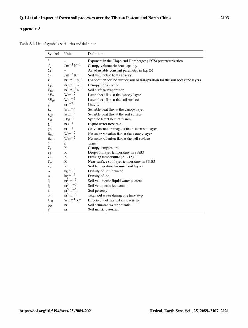
The FSM was implemented in the SSiB3 model to describemulti-layer soil heat transfer and water flow in SSiB3 af-fected by freeze–thaw processes in soil. A schematic of thecoupled model is shown in Fig. 1. The definition of thesymbols in the figure and following equations can be foundin Appendix A. In the soil part, the soil thermal diffusionscheme, soil moisture transport scheme, and freeze–thawscheme are designed to solve the soil thermal diffusion, soilwater diffusion, and ice–liquid phase change, respectively.
The soil column is discretized into 8, 11 and 12 layersfor desert, grassland and trees, respectively. The thickness ofeach soil layer increases with the soil depth, and the depthsof the soil column vary with vegetation types in SSiB3. Thedeepest soil depth also depends on the upper vegetation type.For example, the deepest soil depth over bare soil and grass-land is 7.77 m, and over forest it is about 12 m. The surfacesoil layer was assigned as 2 cm since the variables in the sur-face are sensitive to the atmospheric diurnal forcing.
2.2.1 Energy balance equations
The energy balance equation for the canopy indicates that thecanopy energy storage change with time is affected by the netradiation at the canopy layer and can be written as
Cc∂Tc
∂t= Rnc−Hc− λEc. (1)
The heat budget of the uppermost soil layer is affected bythe net radiation at the soil surface (Rngs; W m−2), sensibleheat (Hgs; W m−2), latent heat fluxes (λEgs; W m−2), energyexchange with lower soil layer and the phase change betweenice and liquid and can be written as
∂(CsTgs
)∂t
−Lilρi∂θi
∂t=
∂
∂Z
(λeff
∂Tgs
∂Z
)+Rngs
−Hgs− λEgs. (2)
Figure 1. Schematic diagram of SSiB3-FSM. Soil temperature, soilvolumetric water content and soil volumetric ice content are T , θland θi, respectively. The heat and water flux between soil layers arerepresented byHk andQk . The soil layer number is k, which rangesfrom 1 to N .
The energy distribution inside the soil column is controlledby the heat conduction between layers and the phase changeinside each individual layer, so it can be written as
∂ (CsTs)
∂t−Lilρi
∂θi
∂t=
∂
∂Z
(λeff
∂Ts
∂Z
). (3)
The first term of Eq. (3) on the left is the heat storage changewith time in each soil layer. The second term is the latentheat due to freezing–thawing. The first term on the right isthe convective heat transferred between the soil layers. At thebottom boundary layer, it is assumed that there is no heat fluxfrom the deeper soil. The differences of energy balance equa-tions for soil between SSiB3 and SSiB3-FSM are the phasechange between ice and liquid
(Lilρi
∂θi∂t
)in the SSiB3-FSM
and directly use the heat conduction equation rather than theforce-restore method.
2.2.2 Water balance equations in soil layers
The water distribution within the soil is driven by the liquidwater movement and liquid–ice phase change. This schemetreats the freeze–thaw process as continuous, without a fixed
2092 Q. Li et al.: Impact of frozen soil processes over the Tibetan Plateau and North China
freezing point, and allows the coexistence of water and ice tomodify the hydraulic and thermal properties of the soil. Theconservation of liquid flow is expressed as a one-dimensionalRichards’ equation:
∂θl
∂t=−
ρi
ρl
∂θi
∂t−∂Ql
∂Z−E. (4)
The liquid water flow rate of Ql (m s−1) is described byDarcy’s law (see Eq. B5 in Appendix B). In the SSiB3-FSM,a freeze–thaw process scheme is used, which is derived fromthe freezing point depression and soil water potential curvein frozen soil:
θl = θs
[LilTs
gψ0Tf(1+Ckθi)
−2]− 1
b
. (5)
This equation has been employed to describe the relation-ships among soil temperature, soil liquid water content, andice content (Li et al., 2010).
2.2.3 Numerical scheme for the thermal andhydrological equations
Equations (1)–(5) are highly nonlinear systems because theice content and liquid water change rapidly with little soiltemperature change during soil freezing or thawing. We pre-viously substituted soil enthalpy and total water mass for soiltemperature and volumetric liquid water content in governingequations (Li et al., 2010) to solve highly nonlinear differ-ential equations. This method also retains energy and waterconservation and represents the continuous and slow energychange in the frozen soil system during the freezing–thawingprocess. However, this approach was only tested for limitedfield sites. While the method was used in the coupled SSiB3-FSM and tested over a global domain, the numerical solu-tions become unstable during the long-term integrations forsome grid points because the global soil properties and me-teorological forcing vary widely. Therefore, a semi-implicitsolution procedure for the soil energy and water prognosticequations was developed with SSiB3-FSM for this study.
Figure 2 presents a flowchart of the semi-implicit solu-tion procedure for SSiB3-FSM. A semi-implicit backwardfinite-difference approximation was used for the thermal dif-fusion equations for canopy and soil (Eqs. 1–3). The numer-ical Eqs. (B1)–(B3) are shown in Appendix B. Meanwhile,Eq. (5) was transformed to a numerical form (B4) so thatit can represent the relationship between the change in soiltemperature (1Ts) and the change in soil ice content (1θi)assuming the total water mass is conserved during one timestep. Then a tridiagonal linear equation system (B5) for thechange in soil temperature was derived based on Eqs. (B1)–(B3), (B4). After solving the tridiagonal matrix at differentsoil layers, the phase change between liquid water and ice(1θi) in soil was decided using the change in soil tempera-ture (1Ts) during one time step (Eq. B4). Because the phase
change has been included while solving the temperature tridi-agonal matrix, here we obtained the soil water content (θi)and soil temperature (Ts) for each soil layer. After the changein ice content has been decided, the water balance equationsdo not involve the prognostic variable of the ice content.Subsequently, we can solve the tridiagonal matrix for wa-ter fluxes at the interface of the soil layers (see Appendix B,Eqs. B6–B10). The liquid water content at the current timestep can be easily obtained from Eq. (B11).
This semi-implicit scheme for soil temperature, liquid wa-ter and ice content in SSiB3-FSM has been tested over theglobal domain. Compared to the previous method that substi-tuted soil enthalpy and total water mass for soil temperatureand volumetric liquid water content, this coupling schemecan effectively produce stable solutions for at least 60 yearsof integrations with the heat and mass balances.
3 Data sets and experimental design
3.1 Data sets
From 1948 to 2007, the SSiB3 model and coupled offlineSSiB3-FSM model were driven using the meteorologicalforcing from the Princeton global meteorological forcingdata set (Sheffield et al., 2006), which is developed by com-bining a suite of global observation-based data sets withthe National Centers for Environmental Prediction/NationalCenter for Atmospheric Research reanalysis data. The dataset includes surface air temperature, pressure, specific hu-midity, wind speed, downward short-wave radiation flux,downward long-wave radiation flux and precipitation. Thespatial resolution is 1◦× 1◦, and the temporal resolution is3 h.
Several observation data sets have been used to evaluatethe performance of SSiB3-FSM and SSiB3 in cold regions.For the surface skin temperature (Tgs), we used the GlobalHistorical Climatology Network version 2 and the ClimateAnomaly Monitoring System (GHCN-CAMS) gauge-based2 m temperature over land for 1979–2007, which providesglobal coverage of monthly means at a regular resolutionof 0.5◦ latitude × 0.5◦ longitude grids (Fan and van denDool, 2008). Although GHCN-CAMS data are air tempera-ture data, in fact the changes in 2 m air temperature are highlyconsistent with those in skin temperature. Therefore, GHCN-CAMS air temperature data were used to validate the simu-lated land surface skin temperature globally.
For the soil temperature profile and the MFD over the TPand NC, the monthly mean soil temperature of 626 stationsover China for 1981–2005 has been used (Yang and Zhang,2016), provided by the China Meteorological Administra-tion (2008). The data set has nine soil layers at 0, 5, 10, 15,20, 40, 80, 160 and 320 cm.
Since the calculation of land soil temperature memory re-quires a long time series of soil temperature data, only the
Q. Li et al.: Impact of frozen soil processes over the Tibetan Plateau and North China 2093
Figure 2. Flowchart of the semi-implicit solution procedure for SSiB3-FSM.
stations with complete records for 1981–2005 and nine soillayers over the TP region (elevation> 2500 m) and NC (110–120◦ E, 34.5–42◦ N) were selected. There are 14 stationsover the TP and 16 sites over NC used for this study. Fig-ure 3 shows the spatial distribution of the stations with avail-able soil temperature data for all nine soil layers and for all12 months of all 25 years over the TP and NC.
3.2 Experimental design and methods
3.2.1 Control run
A global simulation by SSiB3-FSM and SSiB3 was carriedout forced by the Princeton global meteorological forcingdata set from 1948 to 2007. The initial soil temperature andliquid water content profiles were derived by interpolatingthe NCEP-DOE Reanalysis II (R2) (NCEP-R2, Kanamitsuet al., 2002) soil temperature and soil moisture data linearlyto the model’s soil layers. Because the soil ice content mea-surements are unavailable and the initial soil ice content isessential for the soil hydrological and thermal properties, we
set ice content to zero at the beginning. The first 10 years(1948–1957) were used for model spinup, and the simulationfor the last 50 years (1958–2007) was analyzed. The obser-vational data were used to evaluate the model performance,and the results from this run were used to analyze the cold re-gions’ thermal characteristics and MFD as well as their vari-ations under global warming.
3.2.2 Sensitivity run
To investigate the sensitivity of the soil temperature profileand other thermal characteristics to the freeze–thaw process,we conducted a sensitivity simulation using the SSiB3-FSMunder the same initial land surface conditions but without thefreeze–thaw process in soil. This sensitivity run is referredto as the SSiB3-FSMnoICE run hereafter. Both the SSiB3-FSM run and the SSiB3-FSMnoICE run produce multi-layersoil temperature and soil moisture, MFD, net radiation, la-tent heat flux and sensible heat flux as well as the canopytemperature, canopy water and interception.
2094 Q. Li et al.: Impact of frozen soil processes over the Tibetan Plateau and North China
Figure 3. Geographical distribution of stations with complete soil temperature records for all nine soil layers for 1981–2005. The red boxedregion is North China (110–120◦ E, 34.5–42◦ N), and the locations of the 16 sites used in this study are marked by solid circles. The greyline shows that the elevation is above 2500 m, and the grey empty circles denote the locations of the 14 sites on the TP.
3.2.3 Methodology to determine MFD and soil memory
Based on the classification of the permafrost by Frauenfeld etal. (2004), a site was deemed to be seasonally frozen groundwhile the soil temperature at 3.2 m is above 0 ◦C. Based onthis criterion, the 14 stations over the TP and the 16 sitesover NC in this study were all classified as seasonally frozenground. According to the seasonal characteristic of soil tem-perature over seasonally frozen ground, the MFD for eachyear can be defined as an index for the study of seasonalfrozen soil variability and change. This paper gives a prelim-inary estimation of MFD variations based on monthly soiltemperature. Following Frauenfeld et al. (2004), the maxi-mum depth of the zero isothermal line for some year is de-fined as the MFD for this year. Frauenfeld et al. (2004) vali-dated this robustness of this approach. It should be noted thatthe MFD is different from active layer thickness (ALT) be-cause the active layer is defined as “the top layer of groundsubject to annual thawing and freezing in areas underlainby permafrost” (van Everdingen, 1998). ALT is suitable forthe permafrost, but MFD is more suitable for the seasonallyfrozen ground. As the ALT increases, the permafrost thawsdeeper, whereas as the MFD increases, the frozen soil freezesdeeper.
The persistence of soil temperature can be quantified bytemporal scale analysis. Hu and Feng (2004) assumed thatthe temporal variation of the soil enthalpy in North Amer-ica followed the first-order Markov process. Instead of ana-lyzing soil temperature only, the variation of soil enthalpy,which represents integration of soil temperature through thesoil column, was used to examine the land memory (Hu
and Feng, 2004). This study uses the observed and simu-lated soil temperature from ground stations in NC and theTP and the method presented in Entin et al. (2000) and Huand Feng (2004) to analyze the persistence. Land memory ischaracterized by the variable’s autocorrelation, r , satisfyingthe following:
r(δt)= exp(−δt
S
), (6)
in which δt is the time lag, S is the decay timescale that cancharacterize a red noise process and r(δt) is the autocorrela-tion coefficient at the lag time (e.g., 1, 2, 3 months, ... ).
4 Results and discussions
4.1 Assessment of simulated surface 2 m temperatureand temperature profile
4.1.1 Surface 2 m temperature
Before investigating the frozen soil thermal characteristicsand MFD as well as their variability, the SSiB-FSM is firstevaluated using the observational data. The root mean squareerror (RMSE) and absolute bias (BIAS) between CAMS andsimulated surface temperature globally as well as TP and NCfrom the SSiB3-FSM and SSiB3 are assessed (Table 1). Ta-ble 1 shows that the annual RMSE and BIAS of SSiB3-FSMare less than those of SSiB3. In addition, in different sea-sons the SSiB3-FSM shows less bias than SSiB3. Overall,the SSiB3-FSM produces more realistic estimates of surfacetemperature than SSiB3, and it can predict the heat transfer
Q. Li et al.: Impact of frozen soil processes over the Tibetan Plateau and North China 2095
processes globally and locally with a reliable accuracy, whichprovides a basis for further discussions.
4.1.2 Soil temperature profile in the TP
The seasonal vertical soil temperature profile strongly mir-rors the influence of the air temperature forcing, in contrastto the almost isothermal average annual temperature profile(Oelke and Zhang, 2004). The averaged seasonal profiles forobserved soil temperature at 14 sites over the TP are shownin Fig. 4a. For easy comparison, only soil temperature pro-files in January, April, July and October are shown, since thefour curves represent the characteristics of the soil tempera-ture profile in winter, spring, summer and fall, respectively.At the seasonal scale, the surface layer and the subsurfacelayers (here referred to the surface to ∼ 1 m) are frozen dur-ing winter (January), whereas the temperature of the deeplayers (below 1 m) is above 0 ◦C. The surface and subsurfacesoil begins to thaw from March. In April the soil is almostunfrozen. Deep soil temperature always stays above 0 ◦C.
There is a generally rising trend in monthly temperaturefrom winter to summer (from January to July) above 2 m soildepth. Between the 2 and 2.5 m depths there are no appar-ent changes in soil temperature from January to April. Below2.5 m, there is an inverse trend compared with upper soil tem-perature. For instance, the temperature in January is higherthan that in April at 3 m soil depth. From April to July, thetemperature of all soil layers (surface to ∼ 3.2 m) increaseswith the air temperature due to the increasing solar radiation.As the fall approaches, the soil temperature above 1.5 m be-gins to decrease. Below 1.5 m there is a time lag behind therising trend, leading to higher temperature at 3.2 m in Octo-ber than that in July. From October to January, soil tempera-ture in all layers shows a decreasing trend. Generally, the soilis characterized as seasonally frozen ground. Deep soil tem-perature shows a time lag compared with the surface layer,and the upper soil temperature (< 1.5 m) shows larger sea-sonal variability than the deep soil temperature.
The simulated soil temperature profile by SSiB3-FSMover the TP in different seasons is shown in Fig. 4b. Thereis a general consistency between the simulated temperatureprofile and the observed profile in both vertical distributionand the seasonal variations. Compared against observations,however, the simulated soil temperatures underestimate thetemperature in the whole soil column throughout all sea-sons. The air temperature at 2 m in April, July and Octoberin SSiB3-FSM is lower than that observed. This systematicbias arises from the forcing data. For example, the observedair temperature in April at 2 m is about 10 ◦C, but the forcingfor the models is only 6 ◦C. The greatest difference (about6 ◦C) is in July. Considering the forcing data’s bias, we can inparallel move the SSiB3-FSM soil temperature profile to putthe simulated and observed 2 m temperature climatologies inthe same position. Subsequently, the observed and simulatedsoil temperature profiles almost coincided (Fig. 4c).
4.1.3 Soil temperature profile in NC
The simulated and observed seasonal soil temperature pro-files over NC are displayed in Fig. 5a and b, respectively.They show a similar seasonal frozen soil temperature vari-ability to those over the TP, but its thawing season is earlierthan that of the TP. As the observations show, in winter (Jan-uary), the soil freezes above 40 cm, and it begins to thaw inFebruary until March. The soil under 40 cm stays above 0 ◦Cthroughout the year. The simulated temperature profiles andtheir seasonal variations are adequately consistent with theobservations. However, the frozen depth is deeper in SSiB3-FSM than that of the observations in January (Fig. 5c). Thesedifferences may be attributed to the parameterization of soilthermal and hydrological processes in SSiB3-FSM.
4.1.4 Comparison with the force-restore method
In SSiB3 with the force-restore method, only surface tem-perature and deep soil temperature are considered. For theseasonal change in soil temperature, both the seasonal vari-ation of surface soil temperature (Tgs) and deep soil temper-ature (Td) (Fig. 6a and c) are on the same phase, only witha weak lag in Td. It is difficult to define its precise positionof the deep soil temperature layer, which is dependent on thevegetation types and soil conditions. By introducing a multi-layer frozen soil model, SSiB3-FSM not only presents moreprecise soil temperature profile, but also clearly shows theseasonal change in soil temperature at different soil depths(Fig. 6b and d). The time lag and amplitude damping oftemperature become more pronounced with increasing depth,and they are well described in SSiB3-FSM (Fig. 6b and d).This improved performance of SSiB3-FSM lays a founda-tion for further investigation of the characteristics of MFDchanges and soil memory.
4.2 Characteristics of the soil temperature profile overthe TP and NC
4.2.1 Temporal variability of the soil temperatureprofile over the TP and NC
The temporal variability with depth of soil temperature wasfurther explored by analyzing the phase variations withdepth. Here, we used the cross-correlation statistical methodto analyze how the seasonal variability in soil temperaturedecreases with depth. Because the SSiB3-FSM produced rea-sonable surface and subsurface temperature profiles (as dis-cussed in Sect. 4.1) and the observational data are only atmonthly resolution, the 50-year simulated daily soil tempera-tures were used to represent the time–space variability of soiltemperature over a wide area. Figures 7a and 8a show the lagcross-correlations between soil temperature of the first layerwith other layers over the TP and NC, respectively. The timelag at which the maximal correlations occur increases withsoil depth. For instance, the soil layer at 59 cm reaches max-
Figure 4. The seasonal soil temperature profile over the TP (14 sites) for 1981–2005. (a) Observation; (b) simulated by SSiB3-FSM;(c) comparison between the observation and the SSiB3-FSM shifts to the observation climatology.
imum at about 10 d, while the layer at 312 cm needs about90 d (a season). The cross-correlation values decrease af-ter they reach the maximum value and reach zero at about110 and 180 d for the soil layer at 59 and 312 cm, respec-tively. The soil temperature phase lag time was used to moreclearly display these relationships. It is defined as the pointat which the cross-correlation with the first soil layer equals1 (in Figs. 7a and 8a). The change in soil temperature phaselag time with soil depth is shown in Figs. 7b and 8b. Thephase lag time increases linearly with the soil depth, the de-tails of which are presented in Table 2. For the soil depth at1.5 m over the TP, the phase lag for soil temperature is about43 d (∼ 1.5 months). For the soil depth at 3 m, the phase lagcould be 87 d (∼ 3 months). Over NC, the phase lag for soiltemperature is 11 and 32 d at 59 cm and 1.5 m, respectively.
4.2.2 Land memory
The land surface temperature anomaly over the TP and NorthAmerica has been recognized as an indicator of extreme hy-droclimate events (Xue et al., 2018) because of its preser-vation of the snow and other climate signatures in previousmonths. Evaluating the soil persistence of SSiB3 and SSiB3-FSM and comparison with observed soil memory are cru-cial for its application in climate studies. The above anal-ysis of temporal variability in soil temperature with depth
Table 2. Phase lag (days) of simulated soil temperature at differentsoil depths by SSiB3-FSM and SSiB-FSMnoICE.
shows that the soil temperature simulated by SSiB3-FSM ischaracterized by increasing persistence with depth. This sug-gests SSiB3-FSM can be used to study the land persistenceof soil enthalpy, which represents integration of soil temper-ature through the soil column.
Taking the natural log on both sides of Eq. (6) and rear-ranging, we can obtain δt =−S ln[r(δt)], which describesa straight line in the two-dimensional domain of δt and thenatural log of autocorrelation, r . Following this procedure,we calculated autocorrelations of observed monthly soil en-thalpy anomalies between 5 and 320 cm at time lags from 1 to
Q. Li et al.: Impact of frozen soil processes over the Tibetan Plateau and North China 2097
Figure 5. The seasonal soil temperature profile over NC (16 sites) for 1981–2005. (a) Observation; (b) simulated by SSiB3-FSM; (c) obser-vation and SSiB3-FSM.
Figure 6. The seasonal soil temperature simulated by SSiB3 and SSiB-FSM over the TP (14 sites) and NC (16 sites) for 1981–2005. (a) Theseasonal climatology of Tgs (0.02 m) and Td (2.5 m) by SSiB3 over the TP; (b) the seasonal temperature climatology by SSiB3-FSM overthe TP; (c) the seasonal climatology of Tgs (0.02 m) and Td (2.5 m) by SSiB3 over NC, and (d) the seasonal temperature climatology bySSiB3-FSM over NC.
4 months at the 16 stations over NC and 14 sites over the TPand plotted their average autocorrelations in the δt−ln[r(δt)]domain (Fig. 9a and c). The lagged autocorrelations of thesimulated monthly soil enthalpy anomalies at different soillayers between 5 and 312 cm were also calculated and areshown in Fig. 9b and d. The persistence of soil enthalpy
anomalies is determined by the negative inverse of the slopeof the straight line for each case in Fig. 9. The slope of theselines varies, indicating a different persistence time of the soilenthalpy anomaly at different depths.
The persistence values over NC and the TP are given inTable 3. For the observations over NC, the persistence of soil
2098 Q. Li et al.: Impact of frozen soil processes over the Tibetan Plateau and North China
Figure 7. The time–space variability of soil temperature over the TP for 1978–2007. (a) Simulated cross-correlation of the first-layer soiltemperature with other soil layers (red line: 59 cm; purple line: 96 cm; green line: 147 cm; black line: 312 cm) by SSiB3-FSM; (b) the phaselag (days) of simulated temperature over the TP by SSiB3-FSM.
Figure 8. The time–space variability of soil temperature over NC for 1978–2007. (a) Simulated cross-correlation of the first-layer soiltemperature with other soil layers (red line: 59 cm; purple line: 96 cm; green line: 147 cm; black line: 312 cm) by SSiB3-FSM; (b) the phaselag (days) of simulated temperature over NC by SSiB3-FSM.
enthalpy anomalies is about 1.34 months in the top 40 cmcolumn and increases to longer than 2 months in the top160 cm column under the soil surface. In the 320 cm soilcolumn the persistence of soil enthalpy anomalies reaches4.4 months. Similarly, the persistence of simulated soil en-thalpy anomalies is 1.37 months in the 43 cm below the sur-face. It increases to longer than 2 months about the 167 cmsoil column. For the TP, as with NC, both the observedand simulated soil persistence gradually increase with soildepths. The simulated soil persistence below 1.60 m over theTP is larger than the observed one. We will explore the dif-ference in the next study. Generally, over both the TP andNC the observed persistence change with the soil thicknessis reasonably simulated with the SSiB3-FSM.
Table 3. The persistence of soil temperature at different soil depthsover the TP and NC by SSiB3-FSM and the observations.
Q. Li et al.: Impact of frozen soil processes over the Tibetan Plateau and North China 2099
Figure 9. The natural log for the auto-correlation over NC (a, b) and the TP (c, d) for 1981–2005. (a, c) Observed; (b, d) SSiB3-FSM.
The persistence by SSiB3 with the force-restore methodover the TP is only 1.2 and 1.23 months for the surface tem-perature and deep temperature, respectively. For NC, the re-sults by SSiB3 are also about 1 month for the surface temper-ature and deep temperature. SSiB3-FSM shows better perfor-mance in simulating the land persistence for the anomalies insoil than SSiB3, which only considers two layers of temper-ature data.
4.3 Sensitivity of the soil temperature profile to thefreeze–thaw process
A sensitivity experiment, test-SSiB3-FSMnoICE, in whichthe freeze–thaw process in soil is not included, was detailedin Sect. 3.2.2. A comparison of soil temperature profiles wasmade between SSiB3-FSM and SSiB3-FSMnoICE, and theresults are shown in Fig. 10. With freeze–thaw parameteri-zation, the latent heat released while freezing, e.g., in Oc-tober, could offset the decreasing soil temperature. The soiltemperature, therefore, would be higher than that of SSiB3-FSMnoICE. Over the TP, the largest difference is found forJanuary, especially between 50 cm and 1.5 m. The simulatedsoil temperature by SSiB3-FSM is about 1–1.7 ◦C higherthan that by SSiB3-FSMnoICE. Over NC, the large differ-
ences are also shown in winter, especially in January. Thedifference in January is about 1–1.2 ◦C from 15 cm to 1.5 m,which means the freeze process in soil delays the winter cool-ing in freezing seasons (from October to January) and delaysthe summer warming in thawing seasons (from April to July).
The freeze–thaw process has a major impact on soiltemperature profile simulation, especially when freezing orthawing occurs. This effect would exert an impact on thespatial and temporal variability of soil temperature and playan essential role in the soil temperature time lag. Table 2shows that the time lag of SSiB3-FSMnoICE is less thanthat of SSiB3-FSM in almost every soil layer. In particular,over the TP, the difference of lag days between the SSiB3-FSM scheme and SSiB3-FSMnoICE scheme increases withdepth. For instance, at 59 cm, the time lag of the SSiB3-FSM scheme is 3 d longer than that of the SSiB3-FSMnoICEscheme; however, at about 3 m depth, the difference is about15 d. For NC, the freeze–thaw processes also increase thephase lag days even though the number of phase lag days be-tween the SSiB3-FSM and SSiB3-FSMnoICE show less dif-ference than those over the TP in the upper soil depths. Thisis because the maximum freezing depth over NC is about30 cm, much shallower than that over the TP. Correspond-
2100 Q. Li et al.: Impact of frozen soil processes over the Tibetan Plateau and North China
Figure 10. Differences in the seasonal soil temperature profile between the SSiB3-FSMnoICE and SSiB3-FSM for 1981–2005 over (a) theTP (14 sites) and (b) NC (16 sites).
ingly, the effects of the freeze–thaw process are only exertedat shallower soil depths.
4.4 MFD over the TP
The long-term temperature profiles at 14 stations over theTP and 16 sites over NC exhibit characteristics of seasonallyfrozen ground, which freezes in winter and thaws in spring atthe surface soil and remains unfrozen at 3.2 m depth through-out the entire year. The simulated annual soil temporal varia-tions with soil depth over the TP and NC stations are shownin Fig. 11, which displays the seasonal freezing and thawingprocesses during 1981–2005 for the TP and NC. Over the TP,the surface soil starts to freeze in the middle of October andthe MFD occurs around April at 1.8 m. For NC, the surfacesoil starts to freeze at the beginning of December and theMFD occurs in February at around 60 cm soil depth, whichis much shallower than that of the TP.
The MFD at 14 sites over the TP and 16 sites over NC sim-ulated by SSiB3-FSM was averaged to analyze the changesin the MFD for 1981–2005. As for the simulated MFD, itshows large difference from the observational MFD. This dif-ference of MFD between simulation and observation comesfrom the systematic bias of forcing data, just shown in Figs. 4and 5. Therefore, zero-score normalization, which is a com-monly used normalization method, was employed to normal-ize the observed and simulated MFD:
yi =xi − x
s, (7)
x =1n
n∑i=1
xi, s =
√√√√ 1n− 1
n∑i=1
(xi − x)2, (8)
where xi is the original MFD value for 1981–2005 and yi isthe normalized MFD corresponding to xi .
Both the observed MFD over the TP and NC showed asignificant decreasing trend from 1981 to 2005 (Fig. 12).These decreasing trends indicate that, in areas of seasonallyfrozen ground, the freezing ground became increasingly shal-lower during this time period. Over the TP, the observed netchange is a 23 cm decrease in MFD in 2005 compared with1981, and the rate of decrease is about 0.92 cm yr−1. How-ever, from 1983 to 1990 the rate is about 4.5 cm yr−1, whichis about 4 times as much as that in 1981–2005. In the 1990s,the decreasing rate is about 3 cm yr−1. After the 2000s, thedecreasing trend reduced. A similar decrease in the simulatednormalized deviation of MFD at 14 TP sites for 1981–2005is shown in Fig. 12a. The rate of decrease intensified during1983–1990, which was also shown in the observations.
Over NC, the observed decrease in MFD is 13 cmfrom 1981 to 2005. The highest decreasing rate is about3.1 cm yr−1 from 1981 to 1990, about 6 times higher than in1981–2005. The simulated results by SSiB3-FSM also showthe consistency with the observations, especially during the1980s, when the MFD decreasing trend is 1.8 cm yr−1.
The MFD decreasing trend during the 1980s over the TPmay be related to the significant increasing trend in the win-ter and spring air temperature. Wei et al. (2003) analyzedthe inter-decadal variations of air temperature over the TPand found a global climatic jump in the 1980s on the TP,and the air temperature increased more strongly in the win-
Q. Li et al.: Impact of frozen soil processes over the Tibetan Plateau and North China 2101
Figure 11. The climatology of simulated daily soil temperature (a) over the TP (14 sites averaged) and (b) NC (16 sites averaged) for1981–2005 (unit: ◦C).
Figure 12. Normalization of MFD over (a) the TP and (b) NC for 1981–2005 for SSiB3-FSM and the observations.
ter and spring from the 1980s to 2000s. They showed thatthe rates of increasing air temperature at most stations were0.02–0.04 ◦C yr−1 in the winter and spring, which leads to anincreasing trend in the 10–20 cm soil temperature over the TP(Zhang et al., 2008). For NC, an increasing winter tempera-ture trend has been detected since 1985 (Zhang et al., 2002;Shen et al., 2010), which may lead to the decreasing MFDover NC since the 1980s.
It can be seen that the decreasing trend of MFD stabi-lized after 2000. Because MFD was mainly controlled by thewinter surface temperature. Spatio-temporal analysis of sur-face temperature over the TP during 1981–2015 shows thatthe winter surface temperature over the TP increased signif-icantly in the 1980s, and the temperature changes were rela-tively stable in the 1990s and early 21st century (Bai et al.,
2018). That is why the decreasing trend of MFD over the TPafter 2000 is stabilized.
A comparison of MFD between SSiB3-FSM and SSiB3-FSMnoICE was conducted to evaluate the effects of freeze–thaw processes on the MFD. Although the heat and watermass balance due to ice–liquid phase change is not includedin SSiB3-FSMnoICE, the soil temperature still experiences alarge range of variation. Both MFDs show almost the samevariations, but the MFD in SSiB3-FSM is shallower than thatin SSiB3-FSMnoICE (figure not presented). This can be ex-plained by the phase change energy released while freez-ing, which could offset the decreasing temperature duringthe freezing period and lead to a higher soil temperatureat the same soil depth than that simulated by the SSiB3-FSMnoICE.
2102 Q. Li et al.: Impact of frozen soil processes over the Tibetan Plateau and North China
5 Conclusions
To improve the accuracy of soil temperature simulation infrozen ground, a multi-layer FSM was incorporated intoSSiB3 to represent the freezing–thawing process and the heatand water transfer in a multi-layer frozen soil. By introduc-ing a semi-implicit backward finite-difference approximationand a freezing–thawing scheme based on the freezing depres-sion equation, the highly nonlinear equations in multi-layerfrozen soil can be efficiently and stably solved by two tridi-agonal matrixes in SSiB3-FSM. The simulated results showthat with the frozen soil component, the SSiB3-FSM pro-duces realistic soil thermal characteristics than that of SSiB3,especially soil vertical temperature profiles in different sea-sons.
Furthermore, our results confirm the important role offrozen soil processes in soil thermal characteristics at differ-ent timescales over NC and the TP. The results show that thephase-change latent heat released while freezing can offsetthe decreasing soil temperature; therefore, the soil tempera-ture could be higher than that of the experiment without thefrozen soil process as soil freezes. Further analysis of the spa-tial and temporal variability of soil temperature showed thatthe seasonal variability of soil temperature decreases withsoil depths, and the phase lag damps linearly. The frozen soilprocess could increase the phase lag of soil temperature fromseveral days in the surface layer to 15 d in deep layers.
The investigation of SSiB3-FSM’s ability to simulatethe variability of maximum frozen depth at decadal scalesshowed that simulated normalized MFDs over the TP andNC by SSiB3-FSM are in good agreement with the obser-vations for 1981–2005, including the substantial decreasingtrends and the variabilities at decadal scales. The frozen soilprocesses affect the magnitudes but do not change the de-creasing trends of MFD. SSiB3-FSM shows shallower MFDthan SSiB3-FSMnoICE because the simulated soil tempera-ture in SSiB3-FSM is higher than that in SSiB3-FSMnoICE.In addition, the SSiB3-FSM also can reproduce the reliablesoil memory at different soil depths.
The changes in soil properties and their parameterizationshave great effects on the surface energy balance. In partic-ular, the soil thermal conductivity shows large spatial vari-abilities, and the soil thermal properties are heterogeneous inthe vertical direction. A disparity of the soil properties be-tween models and observations may result in the differencebetween the observations and the simulations.
Although the SSiB3-FSM is capable of capturing the ba-sic soil thermal characteristics at seasonal and decadal scalesover regions of seasonally frozen ground, further analy-ses into soil hydrological characteristics in the freezing andthawing phases remain to be conducted. In addition, the bet-ter performance of SSiB3-FSM than that by SSiB3 or SSiB3-FSMnoICE is not only attributed to the frozen soil process,but also to the multi-layer heat and water transfer scheme.The effects of the soil stratification and the soil column depthon the model’s performance over seasonal frozen ground re-quire further study.
Q. Li et al.: Impact of frozen soil processes over the Tibetan Plateau and North China 2103
Appendix A
Table A1. List of symbols with units and definition.
Symbol Units Definition
b – Exponent in the Clapp and Hornberger (1978) parameterizationCc J m−3 K−1 Canopy volumetric heat capacityCk – An adjustable constant parameter in Eq. (5)Cs J m−3 K−1 Soil volumetric heat capacityE m3 m−3 s−1 Evaporation for the surface soil or transpiration for the soil root zone layersEct m3 m−3 s−1 Canopy transpirationEgs m3 m−3 s−1 Soil surface evaporationλEc W m−2 Latent heat flux at the canopy layerλEgs W m−2 Latent heat flux at the soil surfaceg m s−2 GravityHc W m−2 Sensible heat flux at the canopy layerHgs W m−2 Sensible heat flux at the soil surfaceLil J kg−1 Specific latent heat of fusionQl m s−1 Liquid water flow rateqG m s−1 Gravitational drainage at the bottom soil layerRnc W m−2 Net solar radiation flux at the canopy layerRngs W m−2 Net solar radiation flux at the soil surfacet s TimeTc K Canopy temperatureTd K Deep-soil layer temperature in SSiB3Tf K Freezing temperature (273.15)Tgs K Near-surface soil layer temperature in SSiB3Ts K Soil temperature for inner soil layersρl kg m−3 Density of liquid waterρi kg m−3 Density of iceθl m3 m−3 Soil volumetric liquid water contentθi m3 m−3 Soil volumetric ice contentθs m3 m−3 Soil porosityθT m3 m−3 Total soil water during one time stepλeff W m−1 K−1 Effective soil thermal conductivityψ0 m Soil saturated water potentialψ m Soil matric potential
2104 Q. Li et al.: Impact of frozen soil processes over the Tibetan Plateau and North China
Appendix B: Numerical scheme for solving governingequations in SSiB3-FSM
In SSiB3-FSM, a semi-implicit backward finite-differenceapproximation was used for the thermal diffusion in the soil.
For energy balance equation at canopy layer, Eq. (1) canbe written as
Cc1Tc
1t= Rnc+
∂Rnc
∂Tc·1Tc+
∂Rnc
∂Tgs·1Tgs
−Hc−∂Hc
∂Tc·1Tc−
∂Hc
∂Tgs·1Tgs
− λEc− λ∂Ec
∂Tc·1Tc− λ
∂Ec
∂Tgs·1Tgs, (B1)
where 1Tc and 1Tgs denote the change in Tc and Tgs duringa time step.
For groundcover and soil, Eq. (2) can be written as
Cs1Tgs
1t=(Rngs−Hgs− λEgs
)+
(∂Rngs
∂Tc·1Tc+
∂Rngs
∂Tgs·1Tgs
)−
(∂Hgs
∂Tc·1Tc+
∂Hgs
∂Tgs·1Tgs
)−
(λ∂Egs
∂Tc·1Tc− λ
∂Egs
∂Tgs·1Tgs
)+Lilρi
1θi
1t+ 2λeff
T2− Tgs
1z1+1z2. (B2)
For the inner layer, Eq. (3) can be written as
Cs ·1zj ·1Ts,j
1t= Lilρi
1θi,j
1t·1zj
+ 2λeff,jTs,j+1− Ts,j
1zj +1zj+1
− 2λeff,j−1Ts,j − Ts,j−1
1zj−1+1zj. (B3)
Assuming the total water mass is conserved during one timestep, the change in soil temperature (1Ts) and the change insoil ice content (1θi) can be derived based on Eq. (5):
1θi =
(θs)−b(
Lilgψ0Tf
)(1+ ckθi)(θT− θi)
−b[b(θT− θi)
−1 (1+ ckθi)+ 2ck]1Tgs. (B4)
Inserting Eq. (5) into Eqs. (B1)–(B3), the energy balanceequation system can be reorganized as a tridiagonal linearequation system with soil temperature of all the soil layers:
Aj ·1Ts,j−1+Bj ·1Ts,j +Cj ·1Ts,j+1 =Dj , (B5)
where Aj , Bj and Cj are the known coefficients and func-tions of Ts,j−1, Ts,j and Ts,j+1 at the previous time step. Djalso represents the known values at the previous time.
After solving the tridiagonal matrix for the soil temper-ature change at different soil layers, we can obtain the soiltemperature at the current time step (Ts,j ). In addition, thephase change between liquid water and ice in soil can be de-cided using the change in soil temperature during one timestep. Because the phase change has been included while solv-ing the temperature tridiagonal matrix, here we can obtain1θi using Eq. (B4). Then we can solve the water fluxes atthe interface of the soil layers:
Ql,j =Kl,j
[2ψj−ψj+1
Zj +Zj+1+ 1
]. (B6)
Combining Eq. (B6) with Eq. (4), we can obtain water bal-ance equations for the surface layer,
ψk+11 = ψk1 −
1t
Z1
(∂ψ1
∂θl,1Ql,1
)−1t
Z1Egs, (B7)
for the root zone layer,
ψk+1j = ψkj +
1t
Zj
∂ψj
∂θl,j
(Ql,j−1−Ql,j −Ect
), (B8)
and for the bottom soil layer,
ψk+1N = ψkN +
1t
ZN
∂ψN
∂θl,N
(Ql,N−1− qG
). (B9)
Inserting Eqs. (B7)–(B9) into Eq. (B6) and then regroupingEq. (B6), we obtain a tridiagonal linear system for liquid wa-ter flow as follows:
ajQj−1+ bjQj + cjQj+1 = dj , (B10)
where aj , bj and dj are the known coefficients and func-tions of ψj , ψj+1 and θl,j , θl,j+1 at the previous time step.Therefore, the water fluxes at the current time step can besolved using the above tridiagonal matrix. Then the liquidwater content at the current time step can be easily obtainedfrom the following equation:
Q. Li et al.: Impact of frozen soil processes over the Tibetan Plateau and North China 2105
Code and data availability. The SSiB3-FSM code is availableupon request from the first author. The analyses are devel-oped within the Grads and Python software environment. Thescripts are also available upon request from the first author. TheCAMS gridded 2 m temperature is available at https://psl.noaa.gov/data/gridded/data.ghcncams.html (Fan and van den Dool, 2008).The Princeton global meteorological forcing data set is avail-able at http://hydrology.princeton.edu/data.php (Sheffield et al.,2006). The China Ground Temperature Grid Dataset is availableat https://data.cma.cn/data/cdcdetail/dataCode/SURF_CLI_CHN_MUL_MON.html (China Meteorological Administration, 2008).
Author contributions. QL conceived the study and developed themodel. QL and YX developed the framework of the study. QL andYX analyzed all of the simulation results and wrote the paper. QLand YL drafted the figures. All the authors discussed the results andcontributed to finalizing the paper.
Competing interests. The authors declare that they have no conflictof interest.
Acknowledgements. We thank the editor and the reviewers for theirinstructive and insightful comments, which helped to strengthen thispaper.
Financial support. This research has been supported by the Exter-nal Cooperation Program of Bureau of International Cooperation,Chinese Academy of Sciences (grant no. 134111KYSB20200020),the National Key Research and Development Program of China(grant no. 2018YFC1505701) and the National Science Foundationof United States (grant no. AGS-1849654).
Review statement. This paper was edited by Xing Yuan and re-viewed by three anonymous referees.
References
Bai, L., Yao, Y. B., Lei, X. X., and Zhang, L.: Annual and sea-sonal variation characteristics of Surface temperature in the Ti-betan Plateau in recent 40 years, Journal of Geomatics, 43, 15–18, 2018.
Bao, H., Koike, T., Yang, K., Wang, L., Shrestha, M., and Lawford,P.: Development of an enthalpy-based frozen soil model and itsvalidation in a cold region in China, J. Geophys. Res.-Atmos.,121, 5259–5280, https://doi.org/10.1002/2015jd024451, 2016.
Bi, H., Ma, J., Zheng, W., and Zeng, J.: Comparison of soil mois-ture in GLDAS model simulations and in situ observations overthe Tibetan Plateau, J. Geophys. Res.-Atmos., 121, 2658–2678,2016.
Chen, Y., Yang, K., Zhou, D., Qin, J., and Guo, X.: Improving theNoah Land Surface Model in Arid Regions with an AppropriateParameterization of the Thermal Roughness Length, J. Hydrom-
China Meteorological Administration: Dataset of monthly surfaceclimatological data (1951–present) from 613 stations in China,available at: https://data.cma.cn/data/cdcdetail/dataCode/SURF_CLI_CHN_MUL_MON.html (last access: 3 January 2020),2008.
Clapp, R. B. and Hornberger, G. M.: Empirical equations forsome soil hydraulic properties, Water Resour. Res., 14, 601–604,https://doi.org/10.1029/WR014i004p00601, 1978.
Collins, M., Knutti, R., Arblaster, J., Dufresne, J. L., Fichefet, T.,Friedlingstein, P., Gao, X., Gutowski, W. J., Johns, T., Krinner,G., Shongwe, M., Tebaldi, C., Weaver, A. J., and Wehner, M.:Long-term Climate Change: Projections, Com-mitments and Ir-reversibility, in: Climate Change 2013: The Physical Science Ba-sis. Contribution of Working Group I to the Fifth Assessment Re-port of the Intergovernmental Panel on Climate Change, editedby: Stocker, T. F., Qin, D., Plattner, G.-K., Tignor, M., Allen,S. K., Boschung, J., Nauels, A., Xia, Y., Bex, V., and Midgley, P.M., Cambridge University Press, Cambridge, UK and New York,NY, USA, 1029–1136, 2013.
Cuo, L., Zhang, Y., Bohn, T. J., Zhao, L., Li, J., Liu, Q., and Zhou,B.: Frozen soil degradation and its effects on surface hydrologyin the northern Tibetan Plateau, J. Geophys. Res.-Atmos., 120,8276–8298, https://doi.org/10.1002/2015jd023193, 2015.
Deardorff, J. W.: Parameterization of the Planetary Boundary layerfor Use in General Circulation Models, Mon. Weather Rev., 100,93–106, 1972.
Entin, J. K., Robock, A., Vinnikov, K. Y., Hollinger, S.E., Liu, S. X., and Namkhai, A.: Temporal and spa-tial scales of observed soil moisture variations in theextratropics, J. Geophys. Res.-Atmos., 105, 11865–11877,https://doi.org/10.1029/2000jd900051, 2000.
Fan, Y. and van den Dool, H.: A global monthly land surfaceair temperature analysis for 1948–present, J. Geophys. Res.-Atmos., 113, D01103, https://doi.org/10.1029/2007jd008470,2008 (data available at: https://psl.noaa.gov/data/gridded/data.ghcncams.html, last access: 31 January 2021).
Fang, X., Luo, S., and Lyu, S.: Observed soil tempera-ture trends associated with climate change in the TibetanPlateau, 1960–2014, Theor. Appl. Climatol., 135, 169–181,https://doi.org/10.1007/s00704-017-2337-9, 2019.
Flerchinger, G. N. and Saxton, K. E.: Simultaneous heat and watermodel o f a freezing snow-residue-soil system: 1. Theory anddevelopment, Trans. ASAE, 32, 565–571, 1989.
Frauenfeld, O. W., Zhang, T. J., Barry, R. G., and Gilichin-sky, D.: Interdecadal changes in seasonal freeze and thawdepths in Russia, J. Geophys. Res.-Atmos., 109, D05101,https://doi.org/10.1029/2003jd004245, 2004.
Guo, D. L. and Wang, H. J.: Simulation of permafrost and season-ally frozen ground conditions on the Tibetan Plateau, 1981–2010,J. Geophys. Res.-Atmos., 118, 5216–5230, 2013.
Guo, D. and Wang, H.: Simulated change in the near-surface soilfreeze/thaw cycle on the Tibetan Plateau from 1981 to 2010, Chi-nese Sci. Bull., 59, 2439–2448, https://doi.org/10.1007/s11434-014-0347-x, 2014.
Guo, D. and Wang, H.: Simulated Historical (1901–2010) Changesin the Permafrost Extent and Active Layer Thickness in the
2106 Q. Li et al.: Impact of frozen soil processes over the Tibetan Plateau and North China
Northern Hemisphere, J. Geophys. Res.-Atmos., 122, 12285–12295, 2017.
Hu, Q. and Feng, S.: A Role of the Soil Enthalpy in LandMemory, J. Climate, 3633–3643, https://doi.org/10.1175/1520-0442(2004)017<3633:AROTSE>2.0.CO;2, 2004.
Jin, R., Zhang, T., Li, X., Yang, X., and Ran, Y.: Mapping sur-face soil freeze-thaw cycles in China based on SMMR andSSM/I brightness temperatures from 1978 to 2008, Arct. Antarct.Alp. Res., 47, 213–229, https://doi.org/10.1657/aaar00c-13-304,2015.
Kanamitsu, M., Ebisuzaki, W., Woollen, J., Yang, S.-K., Hnilo, J. J.,Fiorino, M., and Potter, G. L.: NCEP-DOE AMIP-II Reanalysis(R-2), Bull. Am. Meteor. Soc., 83, 1631–1643, 2002.
Li, H., Wang, J., and Hao, X.: Influence of Blowing Snow on SnowMass and Energy Exchanges in the Qilian Mountainous, Journalof Glaciology and Geocryology, 34, 1084–1090, 2012.
Li, Q., Sun, S., and Dai, Q.: The Numerical Scheme Development ofa Simplified Frozen Soil Model, Adv. Atmos. Sci., 26, 940–950,2009.
Li, Q., Sun, S., and Xue, Y.: Analyses and development of a hierar-chy of frozen soil models for cold region study, J. Geophys. Res.-Atmos., 115, D03107, https://doi.org/10.1029/2009jd012530,2010.
Li, X., Wu, T., Zhu, X., Jiang, Y., and Ying, X.: Improvingthe Noah-MP Model for Simulating Hydrothermal Regime ofthe Active Layer in the Permafrost Regions of the Qinghai-Tibet Plateau, J. Geophys. Res.-Atmos., 125, e2020JD032588,https://doi.org/10.1029/2020jd032588, 2020.
Liljedahl, A. K., Boike, J., Daanen, R. P., Fedorov, A. N., Frost,G. V., Grosse, G., Hinzman, L. D., Iijma, Y., Jorgenson, J. C.,Matveyeva, N., Necsoiu, M., Raynolds, M. K., Romanovsky, V.E., Schulla, J., Tape, K. D., Walker, D. A., Wilson, C. J., Yabuki,H., and Zona, D.: Pan-Arctic ice-wedge degradation in warmingpermafrost and its influence on tundra hydrology, Nat. Geosci.,9, 312–318, 2016.
Liu, Y., Xue, Y., Li, Q., Lettenmaier, D., and Zhao, P.: Investigationof the Variability of Near-Surface Temperature Anomaly and ItsCauses Over the Tibetan Plateau, J. Geophys. Res.-Atmos., 125,e2020JD032800, https://doi.org/10.1029/2020jd032800, 2020.
Luo, L. F., Robock, A., Vinnikov, K. Y., Schlosser, C. A., Slater,A. G., Boone, A., Braden, H., Cox, P., de Rosnay, P., Dickinson,R. E., Dai, Y. J., Duan, Q. Y., Etchevers, P., Henderson-Sellers,A., Gedney, N., Gusev, Y. M., Habets, F., Kim, J. W., Kowal-czyk, E., Mitchell, K., Nasonova, O. N., Noilhan, J., Pitman, A.J., Schaake, J., Shmakin, A. B., Smirnova, T. G., Wetzel, P., Xue,Y. K., Yang, Z. L., and Zeng, Q. C.: Effects of frozen soil onsoil temperature, spring infiltration, and runoff: Results from thePILPS 2(d) experiment at Valdai, Russia, J. Hydrometeorol., 4,334–351, 2003.
Oelke, C. and Zhang, T.: A model study of circum-arcticsoil temperatures, Permafrost Periglac., 15, 103–121,https://doi.org/10.1002/ppp.485, 2004.
Oelke, C. and Zhang, T.: Modeling the active-layer depth over theTibetan plateau, Arct. Antarct. Alp. Res., 39, 714–722, 2007.
Poutou, E., Krinner, G., Genthon, C., and de Noblet-Ducoudré, N.:Role of soil freezing in future boreal climate change, ClimateDyn., 23, 621–639, https://doi.org/10.1007/s00382-004-0459-0,2004.
Qin, D. H., Zhou, B. T., and Xiao, C. D.: Progress in studies ofcryospheric changes and their impacts on climate of China, J.Meteorol. Res., 28, 732–746, 2014.
Sheffield, J., Goteti, G., and Wood, E. F.: Development of a50-year high-resolution global dataset of meteorological forc-ings for land 50 surface modeling, J. Clim., 19, 3088–3111,https://doi.org/10.1175/jcli3790.1, 2006 (data available at: http://hydrology.princeton.edu/data.php, last access: 31 January 2021).
Shen, H. Y., Ding, Y. G., and Zhang, J.: Inter-decadal varia-tions of winter air temperature in north China and its Circula-tion background, Scientia Meteorologica Sinica, 30, 338–343,https://doi.org/10.3969/j.issn.1009-0827.2010.03.008, 2010.
Slater, A. G., Bohn, T. J., Mc Creight, J. L., Serreze, M. C.,and Lettenmaier, D. P.: A multimodel simulation of pan-Arctic hydrology, J. Geophys. Res.-Biogeo., 112, G04S45,https://doi.org/10.1029/2006jg000303, 2007.
Su, Z., de Rosnay, P., Wen, J., Wang, L., and Zeng, Y.: Evalua-tion of ECMWF’s soil moisture analyses using observations onthe Tibetan Plateau, J. Geophys. Res.-Atmos., 118, 5304–5318,https://doi.org/10.1002/jgrd.50468, 2013.
Sun, S.: Physical, Biochemical Mechanism of Land Surface Processand Its Parameterization, Meterol. Press, Beijing, China, 2005 (inChinese).
Sun, S. and Xue, Y.: Implementing a new snow scheme in simplifiedsimple biosphere model, Adv. Atmos. Sci., 18, 335–354, 2001.
Van Everdingen, R. (Ed.): Multi-language glossary of permafrostand related ground-ice terms (revised May 2005), National Snowand Ice Data Center, Boulder, USA, 1998.
Wei, Z. G., Huang, R., and Dong, W. J.: Interannual and Inter-decadal Variations of Air Temperature and Precipitation over theTibetan Plateau, Chinese Journal of Atmospheric Sciences, 27,157–170, 2003.
Wu, Q. and Zhang, T.: Changes in active layer thickness over theQinghai-Tibetan Plateau from 1995 to 2007, J. Geophys. Res.-Atmos., 115, D09107, https://doi.org/10.1029/2009jd012974,2010.
Xue, Y., Sellers, P. J., Kinter, J. L., and Shukla, J.: A SimplifiedBiosphere Model for Global Climate Studies, J. Clim., 4, 345–364, 1991.
Xue, Y. K., Zeng, F. J., and Schlosser, C. A.: SSiB and its sensitivityto soil properties - A case study using HAPEX-Mobilhy data,Global Planet. Change, 13, 183–194, 1996.
Xue, Y. K., Sun, S. F., Kahan, D. S., and Jiao, Y. J.: Im-pact of parameterizations in snow physics and interface pro-cesses on the simulation of snow cover and runoff at sev-eral cold region sites, J. Geophys. Res.-Atmos., 108, 8859,https://doi.org/10.1029/2002jd003174, 2003.
Xue, Y., Diallo, I., Li, W., David Neelin, J., Chu, P. C., Va-sic, R., Guo, W. D., Li, Q., Robinson, D. A., Zhu, Y. J.,Fu, C. B., and Oaida, C. M.: Spring Land Surface andSubsurface Temperature Anomalies and Subsequent Down-stream Late Spring-Summer Droughts/Floods in North Amer-ica and East Asia, J. Geophys. Res.-Atmos., 123, 5001–5019,https://doi.org/10.1029/2017jd028246, 2018.
Yang, K. and Zhang, J.: Spatiotemporal characteristics of soil tem-perature memory in China from observation, Theor. Appl. Cli-matol., 126, 739–749, 2016.
Q. Li et al.: Impact of frozen soil processes over the Tibetan Plateau and North China 2107
Yang, K., Chen, Y.-Y., and Qin, J.: Some practical notes on the landsurface modeling in the Tibetan Plateau, Hydrol. Earth Syst. Sci.,13, 687–701, https://doi.org/10.5194/hess-13-687-2009, 2009.
Yang, M. X., Nelson, F., Shiklomanov, N., Guo, D. L., and Wan, G.:Permafrost degradation and its environmental effects on the Ti-betan Plateau: A review of recent research, Earth-Sci. Rev., 103,31–44, 2010.
Yang, S., Wu, T., Li, R., Zhu, X., Wang, W., Yu, W., Qin, Y.,and Hao, J.: Spatial-temporal Changes of the Near-surface SoilFreeze-thaw Status over the Qinghai-Tibetan Plateau, PlateauMeteorology, 37, 43–53, 2018.
Yi, S., Wang, X., Qin, Y., Xiang, B., and Ding, Y.: Responsesof alpine grassland on Qinghai–Tibetan plateau to climatewarming and permafrost degradation: a modeling perspective,Environ. Res. Lett., 9, 074014, https://doi.org/10.1088/1748-9326/9/7/074014, 2014.
Zeng, X., Wang, Z., and Wang, A.: Surface Skin Tempera-ture and the Interplay between Sensible and Ground HeatFluxes over Arid Regions, J. Hydrometeorol., 13, 1359–1370,https://doi.org/10.1175/jhm-d-11-0117.1, 2012.
Zhang, G., Nan, Z., Wu, X., Ji, H., and Zhao, S.: TheRole of Winter Warming in Permafrost Change Over theQinghai-Tibet Plateau, Geophys. Res. Lett., 46, 11261–11269,https://doi.org/10.1029/2019gl084292, 2019.
Zhang, T., Barry, R. G., Gilichinsky, D., Bykhovets, S. S.,Sorokovikov, V. A., and Ye, J. P.: An amplified signalof climatic change in soil temperatures during the lastcentury at Irkutsk, Russia, Climatic Change, 49, 41–76,https://doi.org/10.1023/a:1010790203146, 2001.
Zhang, W. G., Li, S. X., and Pang, Q. Q.: Variation Characteristicsof Soil Temperature over Qinghai-Xizang Plateau in the Past 45Years, Acta Geographica Sinica, 63, 1151–1159, 2008.
Zhang, X., Sun, S. F., and Xue, Y. K.: Development and testing of afrozen soil parameterization for cold region studies, J. Hydrom-eteorol., 8, 690–701, 2007.
Zhang, Y., Wang, Q., Qian, Y., and Sun, Y.: Spatial/Temporal Vari-ations of Winter Air Temperature in North China in recent 50Years, Journal of Nanjing Institute of Meteorology, 25, 633–639,2002.
Zhao, D. and Wu, S.: Projected Changes in Permafrost Ac-tive Layer Thickness Over the Qinghai-Tibet Plateau Un-der Climate Change, Water Resour. Res., 55, 7860–7875,https://doi.org/10.1029/2019wr024969, 2019.
Zheng, D., van der Velde, R., Su, Z., Booij, M. J., Hoek-stra, A. Y., and Wen, J.: Assessment of roughness lengthschemes implemented within the Noah land surface modelfor high-altitude regions, J. Hydrometeorol., 15, 921–937,https://doi.org/10.1175/jhm-d-14-0140.1, 2014.
Zheng, D., Van der Velde R., Su, Z., Wen, J., Wang, X.,Booij, M. J., Hoekstra, A. Y., Lv, S., Zhang, Y., and Ek,M. B.: Impacts of Noah model physics on catchment-scalerunoff simulations, J. Geophys. Res.-Atmos., 121, 807–832,https://doi.org/10.1002/2015jd023695, 2016.
Zheng, D., Van der Velde, R., Su, Z., Wen, J., and Wang, X.: As-sessment of Noah land surface model with various runoff param-eterizations over a Tibetan river, J. Geophys. Res.-Atmos., 122,1488–1504, https://doi.org/10.1002/2016jd025572, 2017.