17
The life science business of Merck KGaA, Darmstadt, Germany operates as MilliporeSigma in the U.S. and Canada. Wendy Roe, Richard A. Henry, and Hillel Brandes

The life science business of Merck KGaA, Darmstadt, Germany operates as MilliporeSigma in the U.S. and Canada.
Wendy Roe, Richard A. Henry, and Hillel Brandes

2
Introduction
The HPLC system flow path comprises column plus instrument components that include valves, tubing,
and detector(s). Band spreading occurs as the sample traverses through each component. The band
spreading occurring within the column is minimal and related to the chromatographic process while extra-
column band spreading occurs outside the column and is more rapid and undesirable. Mathematically,
each of the components within the flow path contributes equally to the total observed peak variance as
demonstrated by equation 1. Variances associated with instrument components and tubing are considered
instrument bandwidth (IBW) and require minimization to optimize column performance. As column
diameters decrease, so does the column’s impact in equation 1 rendering the extra-column contributions
more significant to the total system’s performance.
T413131H

3
Capillary HPLC Instrument
•Thermo Scientific UltiMate®
3000 RSLCnano
System (6) (as supplied):
Pump equiped with capillary flow meter
Heated column compartment
UV detector equiped with a 45 nL flow cell
Pulled loop autosampler equiped with a
1 µL sample loop, 2.4 µL needle, and
electronic Peltier elements for sample
cooling
50 µm I.D. tubing connected all
components

4
Measuring Instrument Bandwidth
Several methods exist for the determination of extra-column contributions or
IBW (1-5) in HPLC and UHPLC systems. An adaption is described below.
1. Replace the column with a low volume connector
2. Prepare mobile phase; 40:60 water:acetonitrile
3. Prepare test probe in mobile phase; naphthalene, 55 µg/mL in mobile phase
4. Set detector sampling rate to adequately capture the peak; 25 Hz
5. Inject low sample volumes; 1 µL, 500 nL, 70 nL
6. Record peak efficiency, N, and retention time, tr
7. Calculate σ = (tr x flow) / √N; IBW = 4σ
Experimental
5
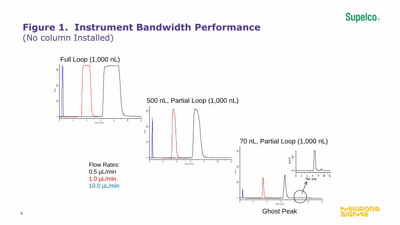
Figure 1. Instrument Bandwidth Performance (No column Installed)
Flow Rates:
0.5 µL/min
1.0 µL/min
10.0 µL/min
Full Loop (1,000 nL)
500 nL, Partial Loop (1,000 nL)
70 nL, Partial Loop (1,000 nL)
Ghost Peak

6
0 2 4 6 8
Time (min)0 2 4 6
Time (min)
Figure 2. Chromatographic Separation Showing Ghost Peaks
300 nL
Injection
70 nL
Injection
Conditions: Column: Acclaim® PepMap™ RSLC C18,
150 mm x 300 µm, 2 µm, Mobile phase: 40:60
water:acetonitrile, Flow rate: 10 µL/min, Column
temperature: 35 ºC, Sample: uracil (7 µg/mL),
acetophenone (7 µg/mL), benzene (750 µg/mL), toluene
(775 µg/mL), naphthalene (55 µg/mL) in 60:40
water:acetonitrile, Detector: UV, 254 nm, Collection rate:
25 Hz, Detector cell volume: 45 nL
Isocratic Method
1 μL Sample Loop, Partial Loop Mode
Conditions: Column: Acclaim PepMap RSLC C18, 150
mm x 300 µm, 2 µm, Mobile phase: (A) water, (B)
acetonitrile, gradient: stepwise 5% B for 1 min, 60% B for
9 min; 0.1 min between steps, Flow rate: 10 µL/min,
Column temperature: 35 ºC, Sample: uracil (7 µg/mL),
acetophenone (7 µg/mL), benzene (750 µg/mL), toluene
(775 µg/mL), naphthalene (55 µg/mL) in 60:40
water:acetonitrile, Detector: UV, 254 nm, Collection rate:
25 Hz, Detector cell volume: 45 nL
Step Gradient Method
1 μL Sample Loop, Partial Loop Mode
70 nL
Injection
Gradient
Step

7
Figure 3. Origin of Ghost Peak from Injection Valve During Partial Loop Injections
Valve switches to load position and partially fills the sample loop. Emptying of sample loop does not completely clear the 1-2 port of sample and allows it to diffuse into sample loop.
Step 1 Step 2
Step 3
Needle (2.4 µL) is filled with sample.
Buffer lineBuffer line
Buffer line
Buffer line
Port to port volume: 348 nL
To SyringeTo Syringe
To Syringe
1 µL Loop1 µL Loop
1 µL Loop
Valve switches to injection position and the 70 nLsample is flushed onto the column. Diffuse sample from port follows the sample band.

8
Figure 4. Effect of Full Loop Injection Volume on System Volume at 0.5 µL/min
0 2 4 6 8 10 12
Time (min)
0100
200
300
mA
U
0 2 4 6 8 10 12
Time (min)
0100
200
300
mA
UInstrument Volume:
6.1 min = 3.1 μL
1,000 nL Injection
Instrument Volume:
5.9 min = 3.0 μL
Sample Volume:
0.5 min = 0.3 μL
Sample Volume:
2.8 min = 1.4 μL
70 nL Injection
Total System Volume:
3.1 μL + 1.4 μL = 4.5
Total System Volume:
3.0 μL + 0.3 μL = 3.3
Peak width taken at baseline

9
Figure 5. IBW for Different Injection Volumes vs. Flow Rate
IBW for different injection volumes vs flow. Mobile phase: 40:60 water:acetonitrile, Column temperature: 35 ºC, Sample: naphthalene, 55 µg/mL in mobile phase, Detector: UV, 254 nm, Collection rate: 25 Hz, Detector cell volume: 45 nL, Chromelon 6.8 used to calculate efficiency.
No column installed; Peak width at half height; IBW = 4σ
1,000 nL
500 nL
70 nL

10
Figure 6. Minimizing Dispersion Through Changing Sample Solvent Strength
Sample Solvent (3 Shown):90:10 Water:Acetonitrile70:30 Water:Acetonitrile40:60 Water:Acetonitrile
Mobile Phase: 40:60 Water:Acetonitrile
Elution Order:1. Uracil2. Acetophenone3. Benzene4. Toluene5. Naphthalene
Conditions: Column: Acclaim PepMap RSLC C18, 150 mm x 300 µm, 2 µm, Mobile phase: 40:60 water:acetonitrile, Flow rate: 10 µL/min, Column temperature: 35 ºC, Injection: Full loop 70 nL, Detector: UV, 254 nm, Collection rate: 25 Hz, Detector cell volume: 45 nL
1.0 2.0 3.0 4.0 5.0 6.0 7.0
Time (min)
1
2
3 4
5
Nnaphthalene= 19,200
Nnaphthalene= 19,300
Nnaphthalene= 17,200
11
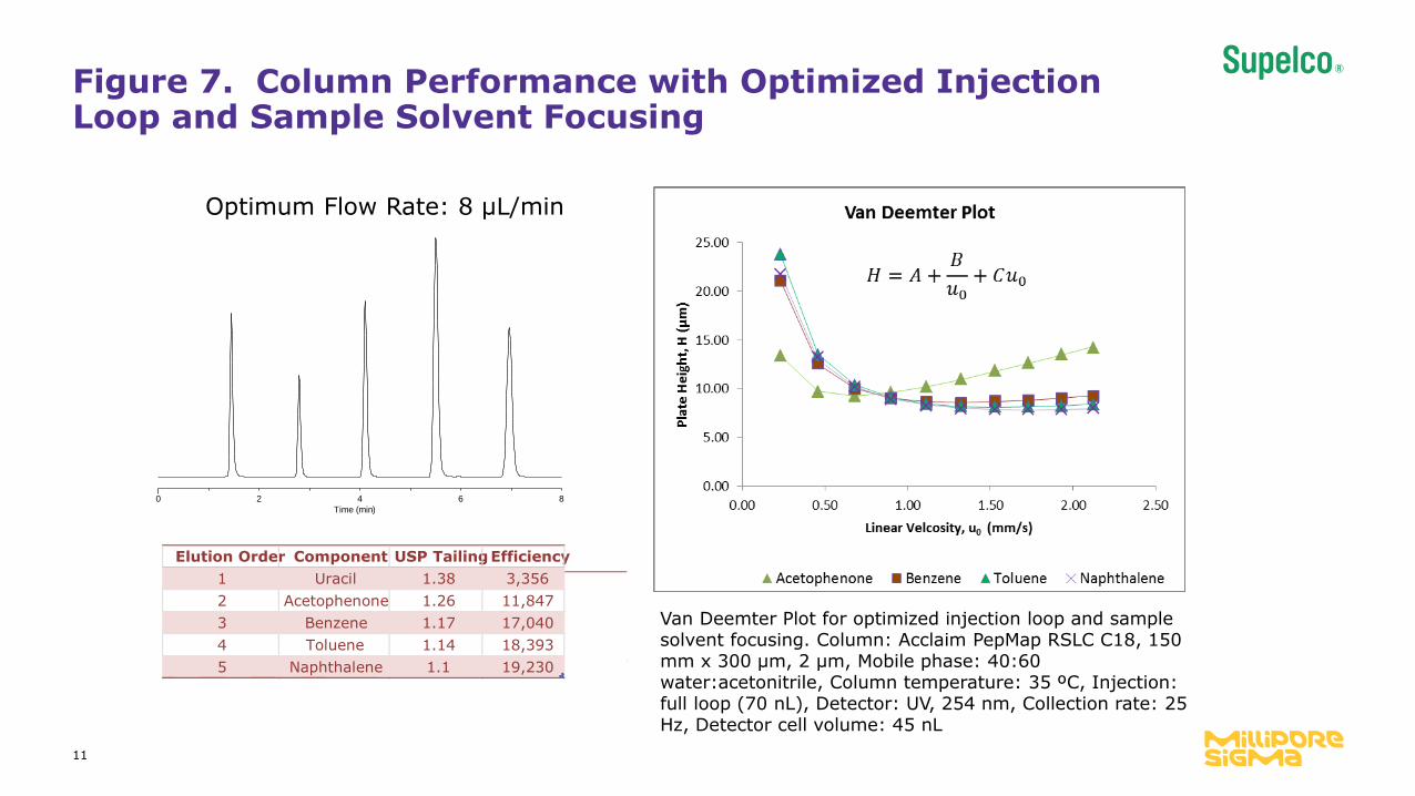
Figure 7. Column Performance with Optimized Injection Loop and Sample Solvent Focusing
Van Deemter Plot for optimized injection loop and sample solvent focusing. Column: Acclaim PepMap RSLC C18, 150 mm x 300 µm, 2 µm, Mobile phase: 40:60 water:acetonitrile, Column temperature: 35 ºC, Injection: full loop (70 nL), Detector: UV, 254 nm, Collection rate: 25 Hz, Detector cell volume: 45 nL
0 2 4 6 8
Time (min)
Optimum Flow Rate: 8 µL/min
Elution Order Component USP TailingEfficiency
1 Uracil 1.38 3,356
2 Acetophenone 1.26 11,847
3 Benzene 1.17 17,040
4 Toluene 1.14 18,393
5 Naphthalene 1.1 19,230

12
Discussion
Figure 1 demonstrates that the largest injection volume exhibited a
square peak shape showing dispersion only at the peak’s leading
and tailing edges. Smaller injection volumes exhibited a normal
Gaussian peak shape.
The smallest injection volume also showed a ghost peak in Figure 1.
To identify the source of this ghost peak, a chromatographic test
using a five component sample was introduced in 300 nL and 70 nL
injection volumes (Figure 2). The 70 nL sample volume showed
ghost peaks for each analyte.
A step gradient performed with the same sample and 70 nL
injection volume exhibited Gaussian peaks for the retained analytes
and the same ghost peak behavior for the void marker (Figure 2).
This indicated that the ghost peaks derived from the injection
process and could be eliminated for retained analytes by focusing
the sample on the top of the column.

13
Consultation with the vendor revealed that the ghost peaks
originated from a diffusion of the sample from the autosampler
valve port. Figure 3 demonstrates the contamination of the sample
loop. First, the needle is filled with sample and the waste is drawn
into the buffer line. When the valve switches to load the sample
loop, the slot connecting ports 6-1 moves to ports 1-2. If not
enough sample is drawn into the sample loop to clear the slot, the
sample diffuses into the backside of the sample loop. It is this
small portion of sample that generates the observed ghost peak(s).
The vendor suggested matching the sample loop volume to the
injection volume. A 30 µm x 100 mm tube (70 nL volume) was
substituted for the 1 µL supplied sample loop and corrected the
ghost peaks at this injection volume. Other design solutions are
currently being investigated to improve all small volume injections.
The 70 nL sample loop was evaluated for dispersion. It exhibited
much lower IBW than the 1,000 nL injection volume and reduced
the total system volume (Figure 4).
Discussion (contd.)

14
Figure 5 summarizes the impact of injection volume on dispersion. As
injection size decreases so does the IBW. The 1 µL sample loop does not
impact the observed IBW, even for 70 nL injections. It is possible to replace
the 1,000 nL sample loop with a 70 nL sample loop and not experience any
additional extra-column effects.
Samples prepared in eluotropically weaker solvents than the mobile phase
focused the sample at the top of the column (Figure 6). This reduced the
sample bandwidth upon entering the column and minimized the extra-column
dispersion ahead of the column. This is evident from the increased efficiency
and improved plate height for naphthalene.
Figure 7 demonstrates the reference column’s performance via a Van Deemter
Plot. The instrument was optimized for small volume injections using a 70 nL
sample loop, and dispersion effects ahead of the column were minimized by a
weak sample solvent. The similar plate heights achieved for the three most
retained analytes indicated the band spreading was effectively minimized to
optimize the column performance.
Discussion (contd.)

15
Conclusions
Choice of sample volumes required careful consideration when using the
Thermo Scientific UltiMate 3000 RSLCnano System. Large sample
volumes, >500 nL, yielded large IBW values. Small sample volumes,
<100 nL, experienced diffusion from the buffer line and required a
smaller volume sample loop to perform well. IBW values for the smaller
sample loop were comparable to the larger sample loop. It is critical to
optimize the sample loop size to the desired sample volume.
Focusing the sample at the entrance to the column minimized the extra-
column dispersion. This technique is recommended for optimal column
performance when using this system for isocratic capillary HPLC
applications. Other systems could benefit from this technique to improve
column performance.
Future experiments to further optimize the system include additional
design changes to improve small volume injections. As hardware changes
are made, further IBW experiments are necessary to ensure extra column
effects are minimized.

16
References
1. R.E. Majors LCGC NORTH AMERICA, Vol. 21 No. 12, 1124-1133 (December 2003).
2. M. W. Dong, Modern HPLC for Practicing Scientists (Wiley-Interscience, New York
2006).
3. F. Gritti, C.A. Sanchez, T. Farkas and G. Guiochon, J. of Chromatography A, 1217,
3000–3012 (2010).
4. R.A. Henry and D. S. Bell, LCGC NORTH AMERICA, Vol. 23 No. 5, 2-7 (May 2005).
5. R. A. Henry, H. K. Brandes, D. T. Nowlan and J. W. Best, Practical Tips for Operating
UHPLC Instruments and Columns, LCGC North America April 2013 (article in press).
6. Dionex website. http://www.dionex.com/en-us/webdocs/57741-Man-LC-U3000-
WPS-PL(RS)+FC-Operation-DOC4828-2050-1-5.pdf (accessed March 1, 2013).

17
Trademarks
Acclaim and UltiMate are registered trademarks of Thermo Fisher Scientific Inc.
PepMap is a trademark of Thermo Fisher Scientific Inc.


![UsingSize-ExclusionChromatographytoMonitorVariationsin …downloads.hindawi.com/journals/isrn.chromatography/2012/... · 2014. 5. 8. · ance liquid chromatography (HPLC) [9], capillary](https://static.documents.pub/doc/80x56/5fca34fca224ec0f6076870b/usingsize-exclusionchromatographytomonitorvariationsin-2014-5-8-ance-liquid.jpg)


