IMPACT OF INTERFERING COMPOUNDS ON THE FERRIC CHLORIDE

ARSENIC REMOVAL TREATMENT PROCESS

By

BENJAMIN HENRY WARE

A thesis submitted in partial fulfillment of

the requirements for the degree of

MASTER OF SCIENCE IN ENVIRONMENTAL ENGINEERING

WASHINGTON STATE UNIVERSITY

Department of Civil & Environmental Engineering

MAY 2013

ii

To the Faculty of Washington State University:

The members of the committee appointed to examine the thesis of BENJAMIN HENRY

WARE find it satisfactory and recommend that it be accepted.

___________________________________

David R. Yonge, Ph.D., Chair

___________________________________

Richard J. Watts, Ph.D.

___________________________________

Marc Beutel, Ph.D.

iii

ACKNOWLEDGMENT

The author would like to thank the following people and organizations for their support

and involvement in this research: Carl Garrison of Garrison Engineering Corp. for funding the

arsenic testing and the members of the Brutus Water System for the opportunity to perform the

tracer study.

iv

IMPACT OF INTERFERING COMPOUNDS ON THE FERRIC CHLORIDE

ARSENIC REMOVAL TREATMENT PROCESS

Abstract

by Benjamin Henry Ware, M.S.

Washington State University

May 2013

Chair: David R. Yonge

Since implementation of the 0.010 mg/L maximum contamination level drinking water

standard for arsenic, many small public water suppliers have been struggling to remain in

compliance. A popular treatment strategy is coagulation/flocculation using ferric chloride

followed by filtration. The presence of phosphate and/or silicate in the source water, however,

has been shown to decrease arsenic removal. The objective of this research was to evaluate

arsenic removal and floc formation as a function of ferric chloride dose, silicate concentration

and phosphate concentration. A synthetic groundwater, developed based on the average

composition of major constituents found in Island County, WA groundwater was used in all

experiments. Field treatment conditions were replicated using standard jar testing equipment to

evaluate the impact of a range of silicate and phosphate concentrations on arsenic removal.

Arsenic concentrations were determined by Inductively Coupled Plasma-Mass Spectrometry. In

synthetic groundwater that contained no phosphate or silicate, arsenic concentrations in filtrate

ranged from 0.004 to 0.002 mg/L (95 to 97 % removal) over the range of iron concentrations

evaluated. Both phosphate and silicate decreased arsenic removal at low iron dosages, resulting

in arsenic concentrations greater than 0.010 mg/L. However, higher iron dosages overcame the

v

interfering compounds effects, reducing arsenic concentrations to levels that were below the

maximum contamination level.

vi

TABLE OF CONTENTS

ACKNOWLEDGMENT ............................................................................................................................................. III

ABSTRACT ............................................................................................................................................................... IV

LIST OF TABLES..................................................................................................................................................... VII

LIST OF FIGURES .................................................................................................................................................. VIII

INTRODUCTION ......................................................................................................................................................... 1

MATERIALS AND METHODS .................................................................................................................................. 5

CHEMICALS. ........................................................................................................................................................ 5

TRACER STUDY. ................................................................................................................................................. 5

SYNTHETIC GROUNDWATER .......................................................................................................................... 6

JAR TESTING PROCEDURE. .............................................................................................................................. 6

ANALYTICAL METHODS. ................................................................................................................................. 7

FACTORIAL EXPERIMENTAL DESIGN. .......................................................................................................... 7

RESULTS AND DISCUSSION .................................................................................................................................. 10

TRACER STUDY. ............................................................................................................................................... 10

IRON BREAKTHROUGH. ................................................................................................................................. 10

PHOSPHATE INTERFERENCE. ........................................................................................................................ 10

SILICATE INTERFERENCE. ............................................................................................................................. 11

COMBINED PHOSPHATE AND SILICATE INTERFERENCE. ..................................................................... 12

CONCLUSIONS ......................................................................................................................................................... 15

FUTURE STUDIES .................................................................................................................................................... 15

REFERENCES ............................................................................................................................................................ 16

APPENDIX ................................................................................................................................................................. 30

vii

LIST OF TABLES

Table 1. Chemical characteristics of synthetic and Island County groundwater .......................... 18

Table 2. An example of calculated values of main effects and interactions and ascending order

sorted main effects and interactions to be plotted in normal probability plot .............................. 18

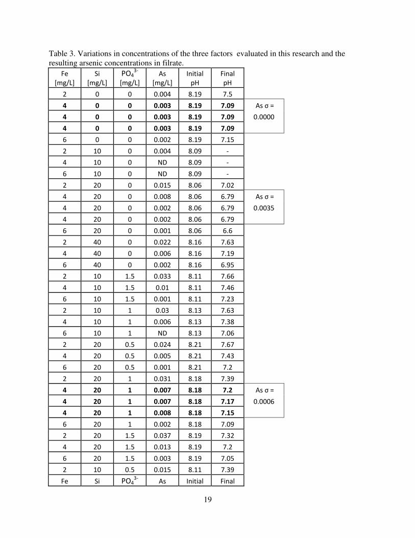
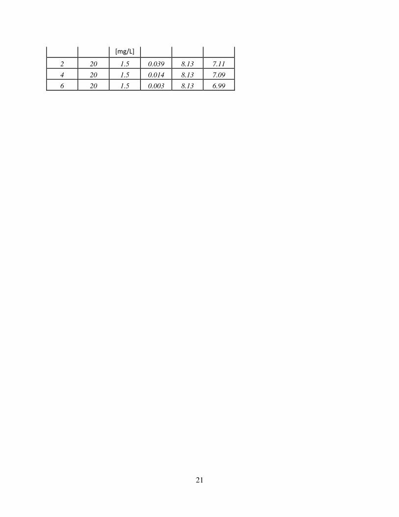
Table 3. Variations in concentrations of the three factors evaluated in this research and the

resulting arsenic concentrations in filrate ..................................................................................... 19

Table 4. The statistically significant average arsenic increases due to increases in phosphate and

silicate concentrations at iron dosages of 2 and 4 mg/L ............................................................... 22

Table 5. The statistically significant average arsenic increases due to increases in phosphate and

silicate concentrations at iron dosages of 4 and 6 mg/L ............................................................... 23

viii

LIST OF FIGURES

Figure 1: Schematic diagram of the Brutus Water System showing NaCl tracer injection loop.. 24

Figure 2: Cube plot of the two level, three factor experimental design. The three factors are Fe

dose, silicate concentration, and phosphate concentration, shown here in high and low levels.

The arsenic responses from the eight experimental conditions are labeled y1 through y8……….24

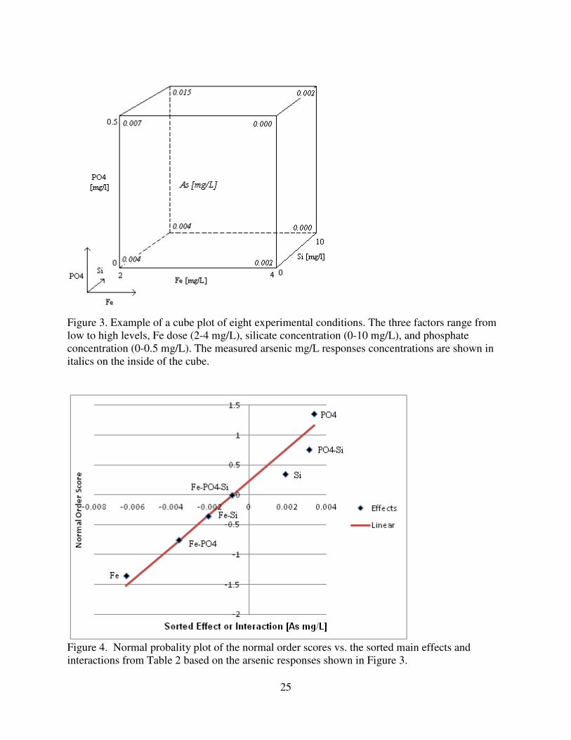
Figure 3: Example of a cube plot of eight experimental conditions. The three factors range from

low to high levels, Fe dose (2-4 mg/L), silicate concentration (0-10 mg/L), and phosphate

concentration (0-0.5 mg/L). The measured arsenic mg/L responses concentrations are shown in

italics on the inside of the cube.. ................................................................................................... 25

Figure 4: Normal probality plot of the normal order scores vs. the sorted main effects and

interactions from Table 2 based on the arsenic responses shown in Figure 3 .............................. 25

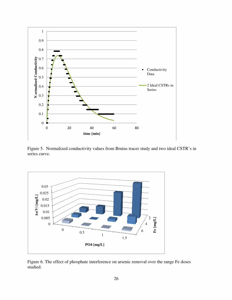
Figure 5: Normalized conductivity values from Brutus tracer study and two ideal CSTR’s in

series curve

....................................................................................................................................................... 26

Figure 6: The effect of phosphate interference on arsenic removal over the range Fe doses

studied.. ......................................................................................................................................... 26

Figure 7: Displays the singular effect of silicates interference on arsenic removal over the range

of Fe doses.. .................................................................................................................................. 27

Figure 8: Arsenic concentrations in filtrate as a function of varying phosphate and silicate

concentrations and a fixed dose of 2 mg/L Fe.. ............................................................................ 27

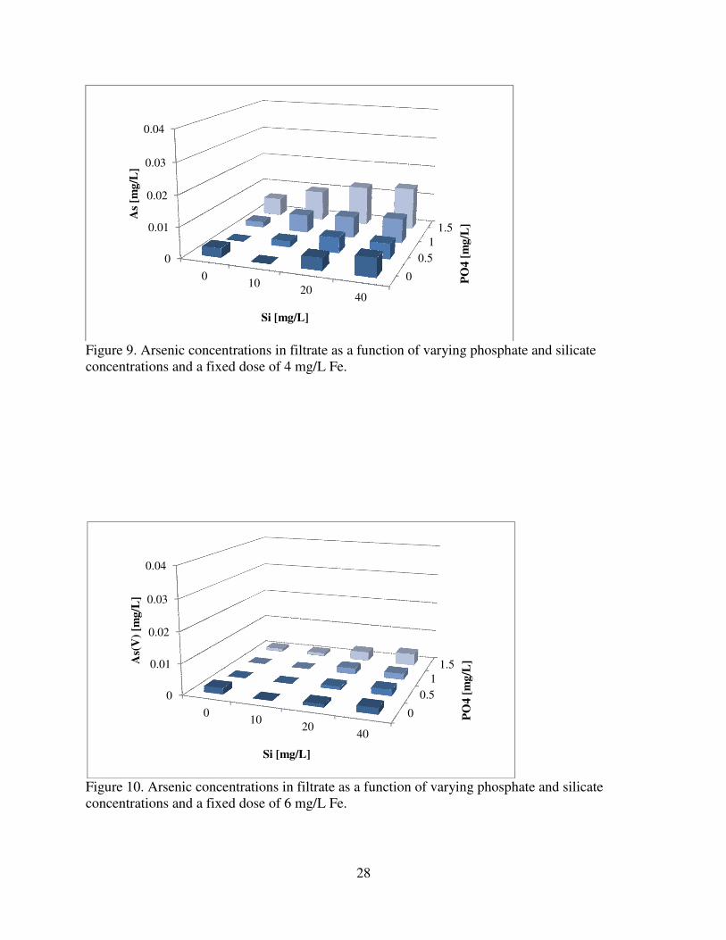
Figure 9: Arsenic concentrations in filtrate as a function of varying phosphate and silicate

concentrations and a fixed dose of 4 mg/L Fe. ............................................................................. 28

Figure 10: Arsenic concentrations in filtrate as a function of varying phosphate and silicate

concentrations and a fixed dose of 6 mg/L Fe. ............................................................................. 28

Figure 11: The original and replicate arsenic removal data .......................................................... 29

ix

DEDICATION

This thesis is dedicated to my family who encouraged me

to work smart not hard.

1

INTRODUCTION

Arsenic is a naturally occurring constituent of groundwater with two common oxidation

states. The reduced form is most often found in groundwater, arsenite (As(III) as AsO33-

), while

the oxidized form, arsenate (As(V) as AsO43-

), predominates in surface waters (USEPA, 2000).

Most waters usually contains a mixture of both As (III) and As(V), and the ratio depends on the

redox condition of the given water. Depending on pH, As(V) exists as a weak acid with

chemical formulas of AsO43-

, HAsO42-

, H2AsO4-, or H3AsO4.

Drinking water containing elevated levels of arsenic is a significant threat to human

health, resulting in both acute and chronic toxic effects. Arsenic attacks DNA ligase and

polymerase that correct mutations in DNA, which increases the risk of cancer initiation, resulting

in cancers of the bladder, kidney, liver, lung, and other organs (USEPA, 2000). Due to the

increased health risk from arsenic exposure, the United States Environmental Protection Agency

(USEPA) and the World Health Organization (WHO) reduced the maximum contamination level

(MCL) of arsenic in drinking water from 50 to 10 µg/L effective in 2006.

Although there are several methods of removing soluble inorganic arsenic from solution,

one of the most popular techniques, and the subject of this research, is chemical coagulation and

flocculation using ferric chloride. Ferric chloride coagulation is an economical form of treatment

and can exhibit high arsenic removal efficiencies, making ferric chloride advantageous for

application in small public treatment systems. Ferric chloride (FeCl3·6H2O) is an inorganic

metal salt that can be purchased in solid or solution form. Once mixed with raw water it

undergoes hydrolysis and forms ferric hydroxide floc. Arsenic forms inner sphere complexes

with ferric hydroxide sites on amorphous ferric hydroxide floc that is then removed by gravity

settling or direct filtration (Meng et al, 2000). Arsenic oxidation state, pH, and coagulate dose

2

affects arsenic removal efficiency (Bilici Baskan et al, 2010). Arsenite adsorption onto iron

hydroxides may only be 5% - 30% that of arsenate adsorptions, therefore, arsenite is normally

oxidized to arsenate before ferric chloride treatment (Chwirka et al, 2004).

One difficulty in meeting the new arsenic MCL using ferric chloride treatment is the

presence of interfering compounds in the raw groundwater. The presence of interfering

compounds has been shown to allow soluble arsenic to pass through filters and into the water

supply. Interfering compounds are also known to increase iron breakthrough in ferric chloride

treatment systems (Meng et al, 2000). Iron breakthrough is defined as the amount of soluble iron

that is not captured in the filter and remains in the treated water. The iron concentration in

drinking water is a secondary water quality standard and should not be exceeded by the addition

of ferric chloride. Arsenic and iron in treated water is both unsafe and aesthetically displeasing

for human consumption. Compounds that interfere with ferric chloride treatment include

phosphate and silicate and the mechanisms of interference for each compound are different.

Phosphate (PO43-

) is most commonly found in the earth’s crust as the mineral apatite,

and is released into groundwater from weathering of apatite or from anthropogenic sources such

as detergents and fertilizer (Matthess, 1982). Due to phosphate’s nearly identical structure and

chemical properties relative to arsenate, phosphate replaces arsenate at iron floc binding sites and

is a competitive inhibitor (Laky et al, 2011; Guan et al, 2009; Roberts et al, 2004). The findings

of Laky et al, (2011) discovered that when phosphate concentrations increased from 0.5 to 1.0

mg/L, an additional 80 percent iron dose was required to lower arsenic concentrations below the

MCL. In addition, if a ferrous salt is used for coagulation, phosphate has been shown to inhibit

the formation of ferric hydroxide floc over a pH range of 7-9 by keeping floc surfaces negative

and preventing the ferric hydroxide floc from growing (Guan et al, 2009).

3

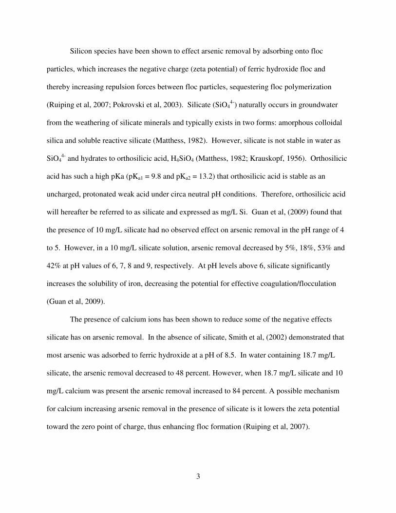
Silicon species have been shown to effect arsenic removal by adsorbing onto floc

particles, which increases the negative charge (zeta potential) of ferric hydroxide floc and

thereby increasing repulsion forces between floc particles, sequestering floc polymerization

(Ruiping et al, 2007; Pokrovski et al, 2003). Silicate (SiO44-

) naturally occurs in groundwater

from the weathering of silicate minerals and typically exists in two forms: amorphous colloidal

silica and soluble reactive silicate (Matthess, 1982). However, silicate is not stable in water as

SiO44-

and hydrates to orthosilicic acid, H4SiO4 (Matthess, 1982; Krauskopf, 1956). Orthosilicic

acid has such a high pKa (pKa1 = 9.8 and pKa2 = 13.2) that orthosilicic acid is stable as an

uncharged, protonated weak acid under circa neutral pH conditions. Therefore, orthosilicic acid

will hereafter be referred to as silicate and expressed as mg/L Si. Guan et al, (2009) found that

the presence of 10 mg/L silicate had no observed effect on arsenic removal in the pH range of 4

to 5. However, in a 10 mg/L silicate solution, arsenic removal decreased by 5%, 18%, 53% and

42% at pH values of 6, 7, 8 and 9, respectively. At pH levels above 6, silicate significantly

increases the solubility of iron, decreasing the potential for effective coagulation/flocculation

(Guan et al, 2009).

The presence of calcium ions has been shown to reduce some of the negative effects

silicate has on arsenic removal. In the absence of silicate, Smith et al, (2002) demonstrated that

most arsenic was adsorbed to ferric hydroxide at a pH of 8.5. In water containing 18.7 mg/L

silicate, the arsenic removal decreased to 48 percent. However, when 18.7 mg/L silicate and 10

mg/L calcium was present the arsenic removal increased to 84 percent. A possible mechanism

for calcium increasing arsenic removal in the presence of silicate is it lowers the zeta potential

toward the zero point of charge, thus enhancing floc formation (Ruiping et al, 2007).

4

It is clear that ferric hydroxide coprecipitation with arsenic can be an effective method of

arsenic removal for small drinking water systems. However, studies indicate that if the raw water

contains phosphate or silicate the arsenic removal may be decreased. Most studies have

investigated the single effect of each interfering compound (Laky et al, 2011; Guan et al, 2009;

Ruiping et al, 2007; Pokrovski et al, 2003). No studies were found that examined the combined

interference of phosphate and silicate on ferric chloride coagulation treatment. Consequently,

this research was focused on both the single and combined effects of phosphate and silicate on

arsenate removal using a simulated groundwater.

5

MATERIALS AND METHODS

Chemicals. All experiments used analytical reagent grade chemicals. Chemicals

included arsenate as HAsNa2O4 ·7H2O (Aldrich Chemistry), ferric chloride as FeCl3 · 6H2O

(Fisher Scientific), silicate as Na2SiO3 · 5H2O (Fisher Scientific), and phosphate as KH2PO4 (J.T.

Baker). Food grade NaCl (Morton Salt, Inc.) was used as an inert tracer to define the hydraulic

characteristics of a field scale treatment system. All stock solutions were prepared using 18 MΩ

deionized water.

Tracer Study. The Brutus Water System (Brutus) supplies drinking water to 28 homes

in Island County, WA and removes arsenic from raw groundwater at an average flow of 14 gpm.

The Brutus treatment system is composed of ferric chloride injection by a flow paced chemical

pump, followed by a KOFLO™ 1 ½” PVC static mixer. The flow then enters through internal

diffuser bars into the bottom of two 120 gallon Flexcon pressurized contact tanks in series and

finally to a filtration unit (Figure 1). To accurately replicate the nominal (actual operating)

hydraulic residence time of the field scale treatment system, an impulse input tracer study of the

ferric chloride treatment process was completed on the Brutus Water System contact tanks. The

nominal residence time gives a more accurate hydraulic residence time than the theoretical

residence (volume/flow rate).

To perform the tracer study on the Brutus Water System, an Eco Testr EC Low

Waterproof Pocket Tester conductivity meter was attached to the sampling port downstream of

ferric hydroxide coagulation/flocculation unit. Background conductivity measurements were

recorded. An injection pipe was then filled with 300 mL of 300 g/L NaCl solution (Figure 1).

Water flow was redirected though the injection pipe to inject the saline tracer solution as an

6

impulse. Time and water conductivity downstream of the tanks were recorded until conductivity

returned to near background levels. Equation 1 was used to estimate the nominal residence time

( t ) (Levenspiel, 1962).

≅ ∑ ∆∑∆

(1)

where =

=

∆ =

Synthetic groundwater. Synthetic groundwater was used in all testing, and was based

on the average constituent concentrations of groundwater found in the arsenic affected areas of

Island Co. Washington (USGS, 1968). The concentrations of constituents are summarized in

Table 1. The synthetic groundwater was prepared by bubbling nanopure DI water with air

overnight or until the pH reached approximately 5.5. To maximize the production of reactive

silicate, solid Na2SiO3 · 5H2O powder was added to 3 L of DI water to achieve final silicate

concentrations of 10, 20 or 40 mg/L as Si. The Na2SiO3 · 5H2O(s) was allowed to dissolve for

30 minutes. After dissolution, the solution pH was about 11. Afterwards 8 mL of Na2CO3 stock

solution (90 g/L) was added, decreasing the solution pH to 9.5. A predetermined amount of

HNO3 was added that ultimately resulted in a final pH of 8.2 ± 0.1. The remaining minerals were

then added to the solution to achieve the concentrations listed in Table 1. Phosphate

concentrations and As(V) were added using 1 g/L stock solutions. The initial As(V)

concentration in the synthetic groundwater was 0.075 mg/L. The synthetic groundwater was then

bubbled with air for 24 hours, which allowed the pH to stabilize to the target value of 8.2.

Jar testing procedure. All tests were conducted at room temperature (~25 °C), and

were open to the atmosphere. Glassware was cleaned by soaking in 10 percent (v/v) HNO3 and

7

rinsed three times with deionized water. One liter of the synthetic groundwater was transferred

into one liter circular Pyrex beakers and set into a standard gang stirrer (Phipps and Bird, PB -

700 JARTESTER) equipped with 1” x 3” rectangular paddles. During the

coagulation/flocculation procedure, ferric chloride was added and flash mixed for 1 minute at

100 rpm yielding a mean velocity gradient (G) of G = 106 s-1

, followed by 20 minutes of slow

mixing (30 rpm; G = 42 s-1

) and then allowed 10 minutes of quiescent settling. The G values

were calculated using data supplied by (Jones et al, 1978).

Following the quiescent settling period, 200 mL of supernatant was collected 4 cm below

the sample surface and was immediately vacuumed filtered through a 1.2 micron glass fiber filter

(Wattman GFC) using Nalgene filter funnels. There was no attempt to control the pH in these

experiments, therefore the final pH of the synthetic groundwater was recorded using a HACH

HQ411d pH meter after the settling period. The floc formation character was evaluated

qualitatively via visual inspection to assess settling rate, floc size and presence of suspended pin

floc. The supernatant was then subjected to As, Fe, and PO43-

analysis.

Analytical methods. Arsenic concentration in the filtrate was analyzed using

Inductively Coupled Plasma Mass Spectrometry (ICP-MS), PO43-

concentrations were analyzed

using stannous chloride method 4500 – P D (Standard Methods, 2005) and Fe concentrations

were determined using HACH method 8008 in conjunction with a spectrophotometer set at a

wave length of 510 nm.

Factorial Experimental Design. Arsenic removal under a range of iron doses (2, 4 and

6 mg/L as Fe), silicate (0, 10, 20, 40 mg/L as Si) and phosphate concentrations (0, 0.5, 1.0, 1.5

mg/L as PO43-

) was evaluated. In order to statistically quantify the effects of these factors and

their concentrations, a two level, three factor experimental design was applied in the data

8

analysis. Since the factorial design uses two concentrations (high and low) for each factor,

multiple factorial analyses were performed in order to cover the entire range of factor

concentrations used herein. The diagram in Figure 2 is an example of one factorial design. The

main effect of each factor was defined as the average change in response (arsenic concentration)

caused by the changing one factor from its low to its high level. A two factor interaction was

defined as a combined effect of the factors on arsenic concentration. After all eight

combinations of factor levels were evaluated via jar testing, each arsenic concentration response

was designated y1 through y8. For example, y4 is a response of arsenic concentration that

resulted from Fe at its high level (+), Si at its low level (-) and PO43-

at its high level (+).

Equations 2 through 8 were used to estimate both the main effects and interactions (Berthouex

and Brown, 1994).

! "#$ % = & + ( + ) + *

4 − + - + . + /4 (2)

12(- "#$ % = - + ( + / + *

4 − + & + . + )4 (3)

4[#/$] =. + ) + / + *4 − + & + - + (

4 (4)

8 ! 12(- "#$ % = + ( + . + *

4 −& + - + ) + /4 (5)

8 ! 4 "#$ % = + - + ) + *

4 −& + ( + . + /4 (6)

8 12(- 4 "#$ % = + & + / + *

4 −- + ( + . + )4 (7)

8 !, 4 12(- "#$ % = & + - + . + *

4 − + ( + ) + /4 (8)

A normal probability plot of the main effects and interactions was made to determine if

the main effects and interactions calculated were significant. If the effects are from randomly

distributed errors then they will form a linear line on the normal probability plot (Berthouex and

9

Brown, 1994). If the data lie off the linear line, the effect or interactions are considered

significant.

For example, Figure 3 shows a factorial design with indicated values of Fe dose, Si and

PO43-

concentrations. To prepare a normal plot, the main effects and interactions were calculated

using equations 2 through 8 and sorted in ascending order, shown in Table 2. In the normal

probability plot, the normal order scores from Teichroew (1956) were plotted versus the sorted

main effects and interactions (Figure 4). Once plotted the data is compared to a line of best fit

and any points on the line are not significant (Fe- PO43-

, Fe-Si, and Fe- PO43-

-Si) and any points

off the line are deemed significant (PO43-

, PO43-

-Si, and Si) shown in Figure 4. This study

investigated three levels of Fe (2, 4, 6 mg/L), and four levels of Si (0, 10, 20, 40 mg/L) and PO43-

(0, 0.5, 1.0, 1.5 mg/L) as shown in Table 3. Therefore, arsenic removal was evaluated over 48

different factor level combinations.

The factorial design does not require replication of the experiments to ensure the

precision of the data. However, triplicates tests were performed at selected conditions to

determine the repeatability of the experiments and are noted in Table 3 as bold font. The

triplicates selected were low Fe, low Si, low PO43-

and medium Fe, medium Si, medium PO43-

and high Fe, high Si, high PO43-

. To ensure that the experiments were reproducible, a second set

of arsenic removal experiments were performed one month later with new stock solutions and

new synthetic groundwater over the range of Fe (2, 4, 6 mg/L), PO43-

(0.5, 1.0, 1.5 mg/L) and a

fixed Si concentration of 20 mg/L. These are the last italic entries in Table 3.

10

RESULTS AND DISCUSSION

Tracer Study. Based on data from the Brutus system tracer study shown in Figure 5, the

two tanks in series treatment system in the field behaved similar to two ideal continuously stirred

tank reactors (CSTR) in series. The treatment system does exhibit some minor dead zones in the

tanks indicated by the longer tail section of the normalized conductivity values compared to the

ideal CSTR curve (Figure 5). The existence of dead zones is not surprising because the

pressurized tanks in the Brutus system are not mechanically stirred, but use an internal diffuser

bar to distribute flow. The nominal (actual) residence time of the treatment system was 19.6

minutes and the theoretical residence time was 17.2 minutes. Despite the effect of dead zones

the nominal residence time was within 14 % of the theoretical residence time, indicating that the

tanks are close to ideal CSTR’s.

Iron Breakthrough. Ferric chloride is an affordable coagulant that effectively removes

arsenic from drinking water in the absence of interfering constituents, which was evident in this

research. In synthetic groundwater that contained no phosphate or silicate the percent arsenic

removal was 95, 96, and 97% for 2, 4, and 6 mg/L iron, respectively. An iron dose of 2 mg/L

was sufficient to lower arsenic concentrations to below MCL standards, yielding a final arsenic

concentration of 0.004 mg/L. No iron breakthrough was observed in this research as all

concentrations were below the HACH 8008 method detection limit of 0.02 mg/L for all

conditions studied. This finding is supported by Laky et al, (2011) who observed iron

breakthrough of 0.015 mg/L iron following filtration through a 0.45 µm pore size membrane in

the presence of 28 mg/L Si.

Phosphate interference. Since phosphate is a competitive inhibitor, it was expected that

high arsenic removal efficiency could be maintained by increasing ferric chloride dose

11

proportional to the phosphate concentration. No visual impact on floc formation was observed

by the presence of phosphate. The results of singular phosphate interference are shown in Figure

6. When synthetic water was dosed with 2 mg/L iron and phosphate levels of 1.0 and 1.5 mg/L,

the final arsenic concentration was 0.021 and 0.030 mg/L arsenic, respectively. An iron dose of

2 mg/L, with no phosphate present, resulted in 95 % arsenic removal, but in the presence of 1.0

and 1.5 mg/L phosphate the arsenic percent removal was reduced to 72 and 60 %, respectively.

However, an iron dose of 4 mg/L (100% dose increase) removed arsenic to below the US EPA

arsenic standard over the range of phosphate levels used in this study. These findings are similar

to results from Laky et al, (2011) who stated that an 80 % increase in iron dose was needed to

reach 0.010 mg/L arsenic in the presence of 1.2 mg/L phosphate.

Silicate interference. Silicate has been reported as a non-competitive inhibitor. Silicate

was believed to not actively compete for binding sites, but act as a dispersant, inhibiting the

formation of ferric hydroxide solids with a resulting increase in soluble arsenic concentrations

(Guan et al, 2009; Pokrovski et al, 2003). The findings of Brandhuber, (2004) observed that

smaller floc was formed as silicate concentration increased. The qualitative data from this study

confirmed that smaller floc was formed in the presence of silicate. Floc formation was delayed

by a few minutes longer in the presence of silicate when compared to the phosphate tests. The

overall floc size was decreased and more pin floc was observed after the settling period.

The results of silicate as a single inhibitor are presented in Figure 7. At silicate

concentrations of 20 and 40 mg/L (as Si), dosed with 2 mg/L iron, observed arsenic

concentrations were 0.015 and 0.022 mg/L, respectively. At the lowest silicate concentration of

10 mg/L, all iron treatment doses removed arsenic to levels below 0.004 mg/L, or 95 percent

removal. Guan et al, (2009) reported only 80 percent arsenic removal in the presence of 10 mg/L

12

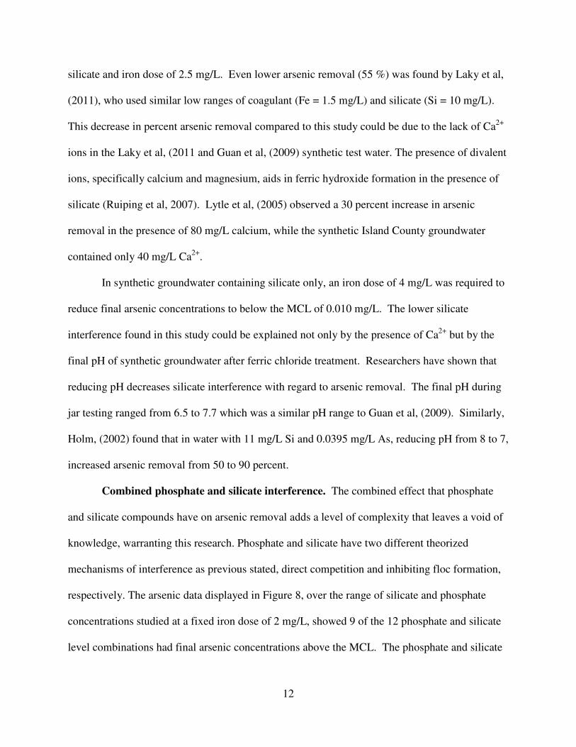
silicate and iron dose of 2.5 mg/L. Even lower arsenic removal (55 %) was found by Laky et al,

(2011), who used similar low ranges of coagulant (Fe = 1.5 mg/L) and silicate (Si = 10 mg/L).

This decrease in percent arsenic removal compared to this study could be due to the lack of Ca2+

ions in the Laky et al, (2011 and Guan et al, (2009) synthetic test water. The presence of divalent

ions, specifically calcium and magnesium, aids in ferric hydroxide formation in the presence of

silicate (Ruiping et al, 2007). Lytle et al, (2005) observed a 30 percent increase in arsenic

removal in the presence of 80 mg/L calcium, while the synthetic Island County groundwater

contained only 40 mg/L Ca2+

.

In synthetic groundwater containing silicate only, an iron dose of 4 mg/L was required to

reduce final arsenic concentrations to below the MCL of 0.010 mg/L. The lower silicate

interference found in this study could be explained not only by the presence of Ca2+

but by the

final pH of synthetic groundwater after ferric chloride treatment. Researchers have shown that

reducing pH decreases silicate interference with regard to arsenic removal. The final pH during

jar testing ranged from 6.5 to 7.7 which was a similar pH range to Guan et al, (2009). Similarly,

Holm, (2002) found that in water with 11 mg/L Si and 0.0395 mg/L As, reducing pH from 8 to 7,

increased arsenic removal from 50 to 90 percent.

Combined phosphate and silicate interference. The combined effect that phosphate

and silicate compounds have on arsenic removal adds a level of complexity that leaves a void of

knowledge, warranting this research. Phosphate and silicate have two different theorized

mechanisms of interference as previous stated, direct competition and inhibiting floc formation,

respectively. The arsenic data displayed in Figure 8, over the range of silicate and phosphate

concentrations studied at a fixed iron dose of 2 mg/L, showed 9 of the 12 phosphate and silicate

level combinations had final arsenic concentrations above the MCL. The phosphate and silicate

13

main effects and phosphate-silicate interaction were evaluated by factorial analysis between the 2

and 4 mg/L iron levels, shown in Table 4.

Contained in Table 4 are all 36 variations of phosphate and silicate levels over the 2 and

4 mg/L iron dose, including their statistical significance and average increase in arsenic response.

The only conditions that had a significant phosphate-silicate interaction was an increase of

phosphate from 0 to 0.5 mg/L and increase of silicate from 0 to 10 mg/L, which increased the

arsenic concentration in the filtrate by an average of 0.003 mg/L (Equation 5). Although only

one significant phosphate-silicate interaction was found, the main effects of phosphate and

silicate were often determined to be significant at iron doses of 2 and 4 mg/L. For example, an

increase of silicate from 0 to 10 mg/L and an increase of phosphate from 0 to 1.5 mg/L resulted

in the main effect of phosphate increasing the arsenic concentration by an average of 0.017 mg/L

(Equation 3). While increasing phosphate levels from 0 to 0.5 mg/L and increasing silicate from

0 to 40 mg/L, the main effect of silicate increased final arsenic concentration by an average of

0.011 mg/L (Equation 4). At all levels of silicate tested the increase of phosphate from 0 to 1.5

mg/L, resulted in a significant increase in final arsenic concentrations. Likewise, over the whole

range of phosphate levels, an increase of 0 to 40 mg/L silicate resulted in a significantly

increased final arsenic concentrations.

Arsenic concentration data shown in Figure 10, at a higher iron dose of 6 mg/L,

overcame the combined interference and removed arsenic to below MCL. However, after

completing factorial analysis between 4 and 6 mg/L iron dose many of the increases in phosphate

and silicate concentration were statistically significant (Table 5). Although these main effects

were statistically significant, the main effect of iron was large enough to lower the effects of

phosphate and silicate and kept arsenic concentration below the MCL.

14

Triplicate data was taken to determine the repeatability of the experiments. The standard

deviation values of the triplicate data in Table 2 are small and range from 0.000 to 0.0035 mg/L

arsenic. Later a replicate set data over the range of iron (2, 4, 6 mg/L), phosphate (0.5, 1.0, 1.5

mg/L) at a fixed silicate concentration of 20 mg/L was performed to determine the

reproducibility of the arsenic removal experiments. The largest deviation between the original

and the replicated set of arsenic removal data was 0.002 mg/L arsenic (Figure 11).

15

CONCLUSIONS

This research was conducted to better understand the combined effect that interfering

compounds have on traditional ferric chloride treatment for arsenic removal. By replicating the

groundwater of Island County, Washington and controlling the concentrations of interfering

compounds, their effect at low iron doses (e.g. 2 mg/L) can decrease arsenic removal from 97 to

59 percent. At a higher iron dose of 4 mg/L the interfering effects are significantly reduced

(Figure 9). The only condition that resulted in arsenic concentrations greater than the MCL of

0.010 mg/L was 20 or 40 mg/L silicate combined with 1.5 mg/L phosphate at an iron dose of 4

mg/L. Although effects of phosphate and silicate were observed on arsenic concentration at an

iron dose of 6 mg/L, all arsenic concentrations were significantly less than 0.010 mg/L.

Consequently, over the range of concentrations studied, increasing iron dose can yield finished

water that meets the 0.010 mg/L MCL.

FUTURE STUDIES

Based on the literature, humic substances have been reported to interfere with arsenic

removal. Therefore future research topics include the effect humic and fulvic acids have on

ferric chloride treatment. Additionally, the combined effects that humic acid with phosphate and

silicate have on arsenic removal efficiency will yield a better understanding of naturally

occurring interfering compounds in marginal groundwater sources. The presence of Ca2+

and

Mg2+

in synthetic groundwater also merits further research because of their capacity to decrease

silicate interference (García-Lara et al, 2010). Calcium or magnesium may also warrant use as

coagulant aids in soft water systems.

16

REFERENCES

Bilici Baskan, M.; Pala, A.; Turkman, A., 2010. Arsenate Removal by Coagulation Using Iron

Salts and Organic Polymers. Ekoloji, 19:74:69.

Berthouex, P.; Brown, L., 1994. Statistics for Environmental Engineers. CRC Press, Boca Raton,

FL.

Brandhuber, P. Impact of the presence of silica on the treatment of arsenic on drinking water.

Proc. 2004 AWWA WQTC.

Chwirka, J.; Colvin, C.; Gomez, J.; Mueller, P., 2004. Arsenic removal from drinking water

using coagulation/microfiltration process. Journal of American Water Works Association,

96:3:106.

García-Lara, A.M.; Montero-Ocampo, C., 2010. Improvement of Arsenic Electro-Removal from

Underground Water by Lowering the Interference of Other Ions. Water Air Soil and

Pollution, 205:1-4:237.

Guan, X.; Dong, H.; Ma, J.; Jiang, L., 2009. Removal of arsenic from water: Effects of

competing anions on As(III) removal in KMnO4–Fe(II) process. Water Research,

43:3891.

Holm, T., 2002. Effects of CO32-

/bicarbonate, Si, and2 PO43-

on Arsenic sorption to HFO.

Journal of American Water Works Association, 94:4:174.

Jones, R.; Williams, R.; Moore, T., 1978. Development and Application of Design and Operation

Procedures for Coagulation of Dredged Material Slurry and Containment Area Effluent.

Environmental Laboratory U.S. Army Engineer Waterways Experiment Station,

Technical Report D-78-54. 1-176.

Krauskopf, K., 1956. Dissolution and precipitation of silica at low temperatures. Geochimica et

Cosmochimica Acta, 10:1-2:1.

Laky, D.; Licskó, I., 2011. Arsenic removal by ferric-chloride coagulation-effect of phosphate,

bicarbonate and silicate. Water Science & Technology, 64:5:1046.

Levenspiel, O., 1962. Chemical Reaction Engineering, John Wiley and Sons, New York, N.Y.

Lytle, D.; Sorg, T.; Snoeyink, V., 2005. Optimizing arsenic removal during iron removal:

Theoretical and practical considerations. Journal of Water: Research & Technology–

AQUA, 54:8:545.

Matthess, G., 1982. The Properties of Groundwater. Trans. John C. Harvey, John Wiley and

Sons, New York, N.Y.

17

Meng, X.; Bang, S.; Korfiatis, G., 2000. Effects of silicate, sulfate, and carbonate on arsenic

removal by ferric chloride. Water Resource 34:4:1255.

Pokrovski, G.; Schott, J.; Farges, F.; Hazemann, J., 2003. Iron (III)-silica interactions in aqueous

solution: Insights from X-ray absorption fine structure spectroscopy. Geochimica et

Cosmochimica Acta, 67:19:3559.

Roberts, L.; Hug, S.; Ruettimann, T.; Billah, M.; Khan, A.; Rahman, M., 2004. Arsenic Removal

with Iron(II) and Iron(III) in Waters with High Silicate and Phosphate Concentrations.

Environmental Science & Technology, 38:1:307.

Ruiping, L,; Xing, L,; Shengji, X,; Yanling, Y,; Rongcheng, W,; Guibal, L., 2007. Calcium-

enhanced ferric hydroxide co-precipitation of arsenic in the presence of silicate. Water

Environment Research, 79:11:2260.

Standard Methods for the Examination of Water and Wastewater. 2005 (21th

ed.). American

Public Health, American Water Works Association, and Water Environment Federation,

Washington.

Smith, S.; Ewards, M. The influence of water quality on arsenate sorption kinetics. Proc. 2002

AWWA WQTC.

Teichroew, D., 1956. Tables of Expected Values of Order Statistics and Products of Order

Statistics for Samples of Size Twenty and Less from the Normal Distribution. The Annals

of Mathematical Statistics, 27:2:410.

USEPA, 2000. “Technologies and Costs for Removal of Arsenic from Drinking Water.” EPA

815-R-00-028 Retrieved from www.epa.gov/safewater

USGS, 1968. Groundwater Resources of Island County. Water Resources Division

VanDenburgh, A. Water Supply Bulletin No. 25, 22-26

18

Table 1. Chemical and physico-chemical characteristics of synthetic and Island County

groundwater.

Synthetic Water Natural Water

pH 8.2 ± 0.1 8

Conductivity [uS/cm] 1060 400

Alkalinity[ mg/L as CaCO3] 125 136

Inorganic Species [mg/L] [meq/L] [mg/L] [meq/L]

Cl- 100 2.82 30 0.85

NO3- 1.3 0.02 1.3 0.02

SO42-

20 0.42 20 0.42

CO32-

136 4.54 140 4.66

∑ = 7.80 ∑ = 5.95

Na+ 105 4.56 60 2.61

K+ 3.3 0.08 3.3 0.08

Mg2+

14.2 1.17 14.2 1.17

Ca2+

40 1.99 40 1.99

∑ = 7.80 ∑ = 5.85

Table 2. An example of calculated values of main effects and interactions and ascending order

sorted main effects and interactions to be plotted in normal probability plot.

Full Factorial Experiment Design 23 Factorial

y1 = 0.004 Effect or

Interaction

Main Effect or

Interaction Eqns 2-8

[As mg/L] Sorted Effect or Interaction

[As mg/L]

Normal

Order

Score

y2 = 0.0025 Fe -0.00638 Fe -0.00638 -1.352

y3 = 0.007 PO43-

0.00338 Fe- PO43-

-0.00363 -0.757

y4 = 0 Si 0.00188 Fe-Si -0.00213 -0.353

y5 = 0.004 Fe- PO43-

-0.00363 Fe- PO43-

-Si -0.00088 0

y6 = 0 Fe-Si -0.00213 Si 0.00188 0.353

y7 = 0.015 PO43-

-Si 0.00313 PO43-

-Si 0.00313 0.757

y8 = 0.002 Fe- PO43-

-Si -0.00088 PO43-

0.00338 1.352

19

Table 3. Variations in concentrations of the three factors evaluated in this research and the

resulting arsenic concentrations in filrate.

Fe

[mg/L]

Si

[mg/L]

PO43-

[mg/L]

As

[mg/L]

Initial

pH

Final

pH

2 0 0 0.004 8.19 7.5

4 0 0 0.003 8.19 7.09 As σ =

4 0 0 0.003 8.19 7.09 0.0000

4 0 0 0.003 8.19 7.09

6 0 0 0.002 8.19 7.15

2 10 0 0.004 8.09 -

4 10 0 ND 8.09 -

6 10 0 ND 8.09 -

2 20 0 0.015 8.06 7.02

4 20 0 0.008 8.06 6.79 As σ =

4 20 0 0.002 8.06 6.79 0.0035

4 20 0 0.002 8.06 6.79

6 20 0 0.001 8.06 6.6

2 40 0 0.022 8.16 7.63

4 40 0 0.006 8.16 7.19

6 40 0 0.002 8.16 6.95

2 10 1.5 0.033 8.11 7.66

4 10 1.5 0.01 8.11 7.46

6 10 1.5 0.001 8.11 7.23

2 10 1 0.03 8.13 7.63

4 10 1 0.006 8.13 7.38

6 10 1 ND 8.13 7.06

2 20 0.5 0.024 8.21 7.67

4 20 0.5 0.005 8.21 7.43

6 20 0.5 0.001 8.21 7.2

2 20 1 0.031 8.18 7.39

4 20 1 0.007 8.18 7.2 As σ =

4 20 1 0.007 8.18 7.17 0.0006

4 20 1 0.008 8.18 7.15

6 20 1 0.002 8.18 7.09

2 20 1.5 0.037 8.19 7.32

4 20 1.5 0.013 8.19 7.2

6 20 1.5 0.003 8.19 7.05

2 10 0.5 0.015 8.11 7.39

Fe Si PO43-

As Initial Final

20

[mg/L] [mg/L] [mg/L] [mg/L] pH pH

4 10 0.5 0.002 8.11 7.14

4 10 0.5 0.002 8.11 7.15

6 10 0.5 ND 8.11 7.02

2 40 0.5 0.023 8.05 7.31

4 40 0.5 0.005 8.05 7.07

6 40 0.5 0.002 8.05 6.92

2 40 1 0.029 8.08 7.27

4 40 1 0.008 8.08 7.07

6 40 1 0.002 8.08 6.87

2 40 1.5 0.037 8.08 7.01

4 40 1.5 0.014 8.08 6.91

6 40 1.5 0.004 8.08 6.81 As σ =

6 40 1.5 0.004 8.08 6.81 0.0000

6 40 1.5 0.004 8.08 6.82

0 0 0 ND - -

2 0 0.5 0.007 8.25 7.65

4 0 0.5 ND 8.25 7.52

6 0 0.5 ND 8.25 7.53

2 0 1 0.021 8.25 7.55

4 0 1 0.002 8.25 7.35

4 0 1 0.002 8.24 7.81

4 0 1 0.002 8.24 7.63

6 0 1 ND 8.24 7.38

2 0 1.5 0.03 8.25 7.55

4 0 1.5 0.006 8.25 7.36

6 0 1.5 0.001 8.25 7.17

2 10 0.5 0.019 8.22 7.4 As σ =

2 10 0.5 0.019 8.22 7.4 0.0000

2 10 0.5 0.019 8.22 7.4

2 20 0.5 0.023 8.15 7.44

4 20 0.5 0.004 8.15 7.32

6 20 0.5 0.001 8.15 7.16

2 20 1 0.032 8.12 7.47

4 20 1 0.007 8.12 7.35 As σ =

4 20 1 0.009 8.12 7.35 0.0010

4 20 1 0.008 8.12 7.35

Fe

[mg/L] Si

[mg/L] PO43-

As

[mg/L] Initial

pH Final

pH

21

[mg/L]

2 20 1.5 0.039 8.13 7.11

4 20 1.5 0.014 8.13 7.09

6 20 1.5 0.003 8.13 6.99

22

Table 4. The statistically significant average arsenic increases due to increases in phosphate and

silicate concentrations at iron dosages of 2 and 4 mg/l.

PO₄ [mg/L] Si [mg/L] PO₄ Main Effect Si Main Effect PO₄-Si Interaction

Cube

# Low High Low High Significant

Average

As

[mg/L] Significant

Average

As

[mg/L] Significant

Average

As

[mg/L]

1 0 0.5 0 10 Yes 0.0034 Yes 0.0020 Yes 0.0031

2 0 0.5 10 20 Yes 0.0058 Yes 0.0068 No -

3 0 0.5 20 40 Yes 0.0025 No - No -

4 0.5 1 0 10 Yes 0.0088 Yes 0.0058 No -

5 0.5 1 10 20 No - No - No -

6 0.5 1 20 40 Yes 0.0046 No - No -

7 1 1.5 0 10 Yes 0.0050 Yes 0.0050 No -

8 1 1.5 10 20 No - No - No -

9 1 1.5 20 40 Yes 0.0064 No - No -

10 0 0.5 0 20 Yes 0.0026 Yes 0.0086 No -

11 0 0.5 0 40 No - Yes 0.0106 No -

12 0 0.5 10 40 No - Yes 0.0086 No -

13 0.5 1 0 20 Yes 0.0063 No - No -

14 0.5 1 0 40 Yes 0.0093 No - No -

15 0.5 1 10 40 No - No - No -

16 1 1.5 0 20 Yes 0.0062 Yes 0.0073 No -

17 1 1.5 0 40 Yes 0.0073 Yes 0.0062 No -

18 1 1.5 10 40 No - No - No -

19 0 1 0 10 Yes 0.0121 No - No -

20 0 1.5 0 10 Yes 0.0171 No - No -

21 0.5 1.5 0 10 Yes 0.0138 No - No -

22 0 1 10 20 Yes 0.0123 No - No -

23 0 1.5 10 20 Yes 0.0175 No - No -

24 0.5 1.5 10 20 Yes 0.0118 No - No -

25 0 1 20 40 Yes 0.0071 Yes 0.0019 No -

26 0 1.5 20 40 Yes 0.0135 No - No -

27 0.5 1.5 20 40 Yes 0.0110 No - No -

28 0 1 0 20 Yes 0.0090 No - No -

29 0.5 1.5 0 20 Yes 0.0125 Yes 0.0090 No -

30 0 1 10 40 Yes 0.0098 Yes 0.0056 No -

31 0.5 1.5 10 40 Yes 0.0123 Yes 0.0048 No -

32 0 1 0 40 Yes 0.0089 No - No -

33 0.5 1.5 0 40 Yes 0.0130 Yes 0.0090 No -

34 0 1.5 10 40 Yes 0.0155 No - No -

35 0 1.5 0 20 Yes 0.0151 Yes 0.0066 No -

36 0 1.5 0 40 Yes 0.0131 No - No -

23

Table 5. The statistically significant average arsenic increases due to increases in phosphate and

silicate concentrations at iron dosages of 2 and 4 mg/l.

PO₄ [mg/L] Si [mg/L] PO₄ Main Effect Si Main Effect

Cube

# Low High Low High Significant

As(V)

[mg/L] Significant

As(V)

[mg/L]

1 0 0.5 0 10 Yes 0.0017 No -

2 0 0.5 10 20 Yes 0.0023 No -

3 0 0.5 20 40 No - No -

4 0.5 1 0 10 Yes 0.0015 Yes 0.0015

5 0.5 1 10 20 Yes 0.0018 Yes 0.0018

6 0.5 1 20 40 Yes 0.0018 No -

7 1 1.5 0 10 Yes 0.0025 No -

8 1 1.5 10 20 No - No -

9 1 1.5 20 40 Yes 0.0036 No -

10 0 0.5 0 20 Yes 0.0016 Yes 0.0014

11 0 0.5 0 40 No - Yes 0.0023

12 0 0.5 10 40 No - Yes 0.0030

13 0.5 1 0 20 No - No -

14 0.5 1 0 40 No - Yes 0.0033

15 0.5 1 10 40 Yes 0.0020 Yes 0.0020

16 1 1.5 0 20 Yes 0.0029 Yes 0.0041

17 1 1.5 0 40 Yes 0.0040 Yes 0.0029

18 1 1.5 10 40 No - Yes 0.0028

19 0 1 0 10 No - No -

20 0 1.5 0 10 Yes 0.0018 Yes 0.0014

21 0.5 1.5 0 10 Yes 0.0040 No -

22 0 1 10 20 No - No -

23 0 1.5 10 20 Yes 0.0055 No -

24 0.5 1.5 10 20 Yes 0.0048 No -

25 0 1 20 40 Yes 0.0016 Yes 0.0010

26 0 1.5 20 40 Yes 0.0053 No -

27 0.5 1.5 20 40 Yes 0.0055 No -

28 0 1 0 20 No - Yes 0.0019

29 0.5 1.5 0 20 No - Yes 0.0038

30 0 1 10 40 No - No -

31 0.5 1.5 10 40 No - No -

32 0 1 0 40 No - Yes 0.0028

33 0.5 1.5 0 40 Yes 0.0048 Yes 0.0043

34 0 1.5 10 40 Yes 0.0053 No -

35 0 1.5 0 20 Yes 0.0034 Yes 0.0024

36 0 1.5 0 40 No - Yes 0.0036

24

Figure 1. Schematic diagram of the Brutus Water System showing NaCl tracer injection loop.

Figure 2. Cube plot of the two level, three factor experimental design. The three factors are Fe

dose, silicate concentration, and phosphate concentration, shown here in high and low levels.

The arsenic responses from the eight experimental conditions are labeled y1 through y8.

25

Figure 3. Example of a cube plot of eight experimental conditions. The three factors range from

low to high levels, Fe dose (2-4 mg/L), silicate concentration (0-10 mg/L), and phosphate

concentration (0-0.5 mg/L). The measured arsenic mg/L responses concentrations are shown in

italics on the inside of the cube.

Figure 4. Normal probality plot of the normal order scores vs. the sorted main effects and

interactions from Table 2 based on the arsenic responses shown in Figure 3.

26

Figure 5. Normalized conductivity values from Brutus tracer study and two ideal CSTR’s in

series curve.

Figure 6. The effect of phosphate interference on arsenic removal over the range Fe doses

studied.

0

0.1

0.2

0.3

0.4

0.5

0.6

0.7

0.8

0.9

1

0 20 40 60 80

N o

rma

lize

d C

on

du

ctiv

ity

time [min]

Conductivity

Data

2 Ideal CSTRs in

Series

2

4

6

0

0.005

0.01

0.015

0.02

0.025

0.03

00.5

11.5

Fe

[mg

/L]

As(

V)

[mg

/L]

PO4 [mg/L]

27

Figure 7. The effect of silicates interference on arsenic removal over the range of Fe doses

studied.

Figure 8. Arsenic concentrations in filtrate as a function of varying phosphate and silicate

concentrations and a fixed dose of 2 mg/L Fe.

2

4

6

0

0.005

0.01

0.015

0.02

0.025

0.03

010

2040

Fe

[mg

/L]

As(

V)

[mg

/L]

Si [mg/L]

0

0.5

1

1.5

0

0.005

0.01

0.015

0.02

0.025

0.03

0.035

0.04

010

2040

PO

4 (

mg

/L)

As

(mg

/L)

Silicate (mg/L)

28

Figure 9. Arsenic concentrations in filtrate as a function of varying phosphate and silicate

concentrations and a fixed dose of 4 mg/L Fe.

Figure 10. Arsenic concentrations in filtrate as a function of varying phosphate and silicate

concentrations and a fixed dose of 6 mg/L Fe.

0

0.5

1

1.5

0

0.01

0.02

0.03

0.04

010

2040

PO

4 [

mg

/L]

As

[mg

/L]

Si [mg/L]

0

0.5

1

1.5

0

0.01

0.02

0.03

0.04

010

2040

PO

4 [

mg

/L]A

s(V

) [m

g/L

]

Si [mg/L]

29

Figure 11. The original and replicate arsenic removal data, each pair was within 0.002 mg/L

arsenic.

0

0.005

0.01

0.015

0.02

0.025

0.03

0.035

0.04

0.045

1 2 3 4 5 6 7

As

[mg

/L]

Fe [mg/L]

Original 0.5

Original 1.0

Original 1.5

Duplicate 0.5

Duplicate 1.0

Duplicate 1.5

APPENDIX

31

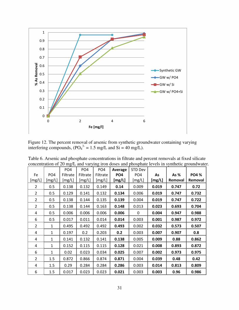
Figure 12. The percent removal of arsenic from synthetic groundwater containing varying

interfering compounds, (PO43-

= 1.5 mg/L and Si = 40 mg/L).

Table 6. Arsenic and phosphate concentrations in filtrate and percent removals at fixed silicate

concentration of 20 mg/L and varying iron doses and phosphate levels in synthetic groundwater.

Fe

[mg/L]

PO4

[mg/L]

PO4

Filtrate

[mg/L]

PO4

Filtrate

[mg/L]

PO4

Filtrate

[mg/L]

Average

PO4

[mg/L]

STD Dev

PO4

[mg/L]

As

[mg/L] As %

Removal PO4 %

Removal

2 0.5 0.138 0.132 0.149 0.14 0.009 0.019 0.747 0.72

2 0.5 0.129 0.141 0.132 0.134 0.006 0.019 0.747 0.732

2 0.5 0.138 0.144 0.135 0.139 0.004 0.019 0.747 0.722

2 0.5 0.138 0.144 0.163 0.148 0.013 0.023 0.693 0.704

4 0.5 0.006 0.006 0.006 0.006 0 0.004 0.947 0.988

6 0.5 0.017 0.011 0.014 0.014 0.003 0.001 0.987 0.972

2 1 0.495 0.492 0.492 0.493 0.002 0.032 0.573 0.507

4 1 0.197 0.2 0.203 0.2 0.003 0.007 0.907 0.8

4 1 0.141 0.132 0.141 0.138 0.005 0.009 0.88 0.862

4 1 0.152 0.115 0.115 0.128 0.021 0.008 0.893 0.872

6 1 0.02 0.023 0.034 0.025 0.007 0.002 0.973 0.975

2 1.5 0.872 0.866 0.874 0.871 0.004 0.039 0.48 0.42

4 1.5 0.29 0.284 0.284 0.286 0.003 0.014 0.813 0.809

6 1.5 0.017 0.023 0.023 0.021 0.003 0.003 0.96 0.986

0

0.1

0.2

0.3

0.4

0.5

0.6

0.7

0.8

0.9

1

0 2 4 6

% A

s R

em

ov

al

Fe [mg/l]

Synthetic GW

GW w/ PO4

GW w/ Si

GW w/ PO4+Si

32

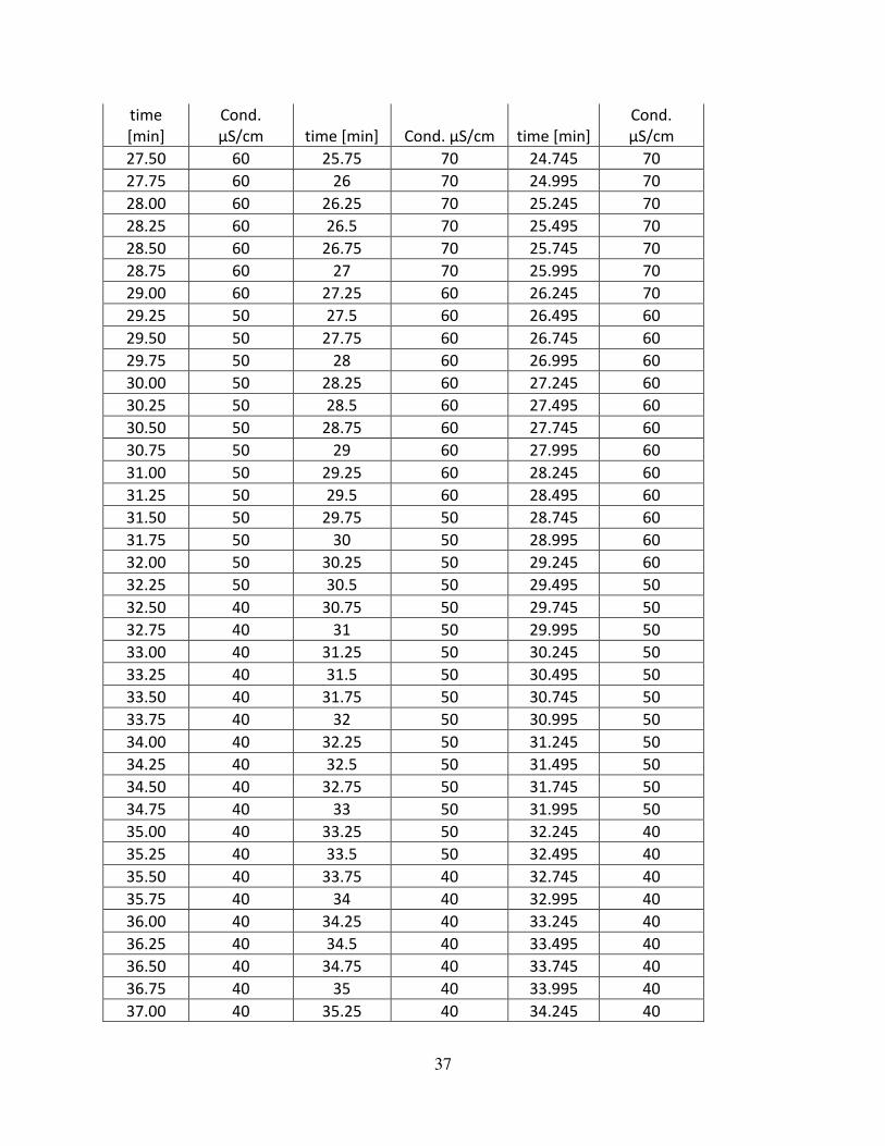
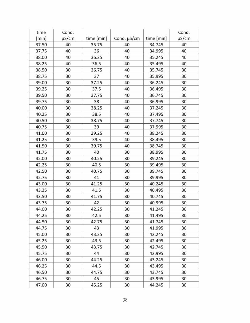
Table 7. Raw tracer study data conductivity and time

Test 1 Test 2 Test 3

time

[min]

Cond.

μS/cm time [min] Cond. μS/cm time [min]

Cond.

μS/cm

0.000 0 0.000 0 0.000 0

0.083 0 0.083 0 0.083 0

0.167 0 0.167 0 0.167 0

0.250 0 0.250 0 0.250 0

0.333 0 0.333 0 0.333 0

0.417 0 0.417 0 0.417 0

0.500 0 0.500 0 0.500 0

0.583 0 0.583 0 0.583 0

0.667 0 0.667 0 0.666 0

0.750 0 0.750 0 0.750 10

0.833 10 0.833 10 0.833 10

0.917 20 0.917 20 0.916 10

1.000 20 1.000 30 1.000 10

1.083 20 1.083 40 1.083 10

1.167 20 1.167 60 1.166 30

1.250 30 1.250 60 1.250 40

1.333 40 1.333 60 1.333 40

1.417 40 1.417 60 1.416 50

1.500 40 1.500 60 1.499 50

1.583 40 1.583 60 1.583 50

1.667 50 1.667 60 1.666 60

1.750 60 1.750 60 1.749 60

1.833 60 1.833 60 1.833 60

1.917 70 1.917 60 1.916 70

2.000 80 2.000 60 1.999 70

2.083 80 2.083 60 2.083 70

2.167 80 2.167 70 2.166 80

2.250 80 2.250 70 2.249 80

2.333 80 2.333 70 2.332 80

2.417 80 2.417 70 2.416 80

2.500 80 2.500 70 2.499 80

2.583 80 2.583 80 2.582 80

2.667 80 2.667 90 2.666 80

2.750 90 2.750 100 2.749 80

2.833 100 2.833 100 2.832 90

2.917 100 2.917 100 2.916 90

3.000 100 3.000 100 2.999 100

33

time

[min]

Cond.

μS/cm time [min] Cond. μS/cm time [min]

Cond.

μS/cm

3.167 100 3.167 110 3.165 100

3.250 100 3.250 120 3.249 100

3.333 100 3.333 120 3.332 100

3.417 110 3.417 120 3.415 100

3.500 110 3.500 120 3.499 100

3.583 110 3.583 120 3.582 100

3.667 110 3.667 120 3.665 100

3.750 120 3.750 120 3.749 100

3.833 120 3.833 120 3.832 100

3.917 120 3.917 120 3.915 100

4.000 120 4.000 120 3.998 110

4.083 120 4.083 130 4.082 110

4.167 120 4.167 130 4.165 110

4.250 120 4.250 130 4.248 120

4.333 120 4.333 140 4.332 120

4.416 120 4.416 140 4.415 120

4.500 130 4.500 140 4.498 130

4.583 130 4.583 140 4.582 130

4.666 130 4.666 140 4.665 140

4.750 140 4.750 140 4.748 140

4.833 140 4.833 140 4.831 140

4.916 140 4.916 150 4.915 140

5.000 140 5.000 150 4.998 140

5.083 140 5.083 150 5.081 140

5.166 140 5.166 150 5.165 140

5.250 140 5.250 150 5.248 140

5.333 140 5.333 150 5.331 140

5.416 140 5.416 150 5.415 140

5.500 140 5.500 150 5.498 150

5.583 150 5.583 150 5.581 150

5.666 150 5.666 150 5.664 150

5.750 150 5.750 150 5.748 150

5.833 150 5.833 160 5.831 150

5.916 150 5.916 160 5.914 150

6.000 150 6.000 160 5.998 150

6.083 150 6.083 160 6.081 150

6.166 150 6.166 160 6.164 150

6.250 160 6.250 160 6.248 150

6.333 160 6.333 160 6.331 150

34

time

[min]

Cond.

μS/cm time [min] Cond. μS/cm time [min]

Cond.

μS/cm

6.583 160 6.583 160 6.581 150

6.666 160 6.666 160 6.664 160

6.750 160 6.750 160 6.747 160

6.833 160 6.833 160 6.831 160

6.916 160 6.916 160 6.914 160

7.000 160 7.000 160 6.997 160

7.083 160 7.083 160 7.081 160

7.166 160 7.166 160 7.164 160

7.250 160 7.250 160 7.247 160

7.333 160 7.333 160 7.330 160

7.416 160 7.416 160 7.414 160

7.500 160 7.500 160 7.497 160

7.583 160 7.583 170 7.580 160

7.666 160 7.666 170 7.664 160

7.750 160 7.750 170 7.747 160

7.833 160 7.833 170 7.830 160

7.916 160 7.916 170 7.914 160

8.000 160 8.000 170 7.997 160

8.083 160 8.083 170 8.080 160

8.166 160 8.166 170 8.163 160

8.250 160 8.250 170 8.247 160

8.333 160 8.333 170 8.330 160

8.416 160 8.416 170 8.413 160

8.500 160 8.500 170 8.497 160

8.583 160 8.583 170 8.580 160

8.666 160 8.666 170 8.663 160

8.750 160 8.750 170 8.747 160

8.833 160 8.833 170 8.830 160

8.916 160 8.916 170 8.913 160

9.000 160 9.000 170 8.996 160

9.083 160 9.083 170 9.080 160

9.166 160 9.166 170 9.163 160

9.250 160 9.250 170 9.246 160

9.333 160 9.333 170 9.330 160

9.416 160 9.416 170 9.413 160

9.500 160 9.500 170 9.496 160

9.583 160 9.583 170 9.580 160

9.666 160 9.666 170 9.663 160

9.750 160 9.750 170 9.746 160

35

time

[min]

Cond.

μS/cm time [min] Cond. μS/cm time [min]

Cond.

μS/cm

9.916 160 9.916 170 9.913 160

10.000 160 10.000 170 9.996 160

10.083 160 10.083 170 10.079 160

10.166 160 10.166 170 10.163 160

10.250 160 10.250 170 10.246 160

10.333 160 10.333 170 10.329 160

10.416 160 10.416 170 10.413 160

10.500 160 10.500 170 10.496 160

10.583 160 10.583 160 10.579 160

10.666 160 10.666 160 10.662 160

10.750 160 10.750 160 10.746 160

10.833 160 10.833 160 10.829 160

10.916 160 10.916 160 10.912 160

11.000 160 11.000 160 10.996 160

11.083 160 11.083 160 11.079 160

11.166 160 11.166 160 11.162 160

11.250 160 11.250 160 11.246 150

11.333 160 11.333 160 11.329 150

11.416 160 11.416 160 11.412 150

11.500 160 11.500 160 11.495 150

11.583 160 11.583 160 11.579 150

11.666 160 11.666 160 11.662 150

11.750 150 11.750 160 11.745 150

11.833 150 11.833 160 11.829 150

11.916 150 11.916 160 11.912 150

12.000 150 12 160 11.995 150

13.750 140 12.25 150 12.079 150

14.083 140 12.5 150 12.162 150

14.167 140 12.75 150 12.245 150

14.750 140 13 150 12.328 150

15.00 140 13.25 150 12.412 150

15.25 140 13.5 150 12.495 150

15.50 140 13.75 150 12.745 150

15.75 130 14 150 12.995 150

16.00 130 14.25 140 13.245 150

16.25 130 14.5 140 13.495 140

16.50 130 14.75 140 13.745 140

16.75 120 15 140 13.995 140

17.00 120 15.25 140 14.245 140

36

time

[min]

Cond.

μS/cm time [min] Cond. μS/cm time [min]

Cond.

μS/cm

17.50 120 15.75 130 14.745 140

17.75 120 16 130 14.995 130

18.00 120 16.25 130 15.245 130

18.25 110 16.5 130 15.495 130

18.50 110 16.75 130 15.745 130

18.75 110 17 120 15.995 130

19.00 110 17.25 120 16.245 130

19.25 110 17.5 120 16.495 120

19.50 110 17.75 120 16.745 120

19.75 110 18 120 16.995 120

20.00 100 18.25 120 17.245 120

20.25 100 18.5 110 17.495 120

20.50 100 18.75 110 17.745 110

20.75 100 19 110 17.995 110

21.00 100 19.25 110 18.245 110

21.25 90 19.5 110 18.495 110

21.50 90 19.75 100 18.745 110

21.75 90 20 100 18.995 110

22.00 90 20.25 100 19.245 110

22.25 90 20.5 100 19.495 100

22.50 90 20.75 100 19.745 100

22.75 90 21 100 19.995 100

23.00 80 21.25 100 20.245 100

23.25 80 21.5 90 20.495 100

23.50 80 21.75 90 20.745 90

23.75 80 22 90 20.995 90

24.00 80 22.25 90 21.245 90

24.25 80 22.5 90 21.495 90

24.50 80 22.75 90 21.745 90

24.75 80 23 80 21.995 90

25.00 80 23.25 80 22.245 90

25.25 70 23.5 80 22.495 80

25.50 70 23.75 80 22.745 80

25.75 70 24 80 22.995 80

26.00 70 24.25 80 23.245 80

26.25 70 24.5 80 23.495 80

26.50 70 24.75 70 23.745 80

26.75 60 25 70 23.995 80

27.00 60 25.25 70 24.245 80

37

time

[min]

Cond.

μS/cm time [min] Cond. μS/cm time [min]

Cond.

μS/cm

27.50 60 25.75 70 24.745 70

27.75 60 26 70 24.995 70

28.00 60 26.25 70 25.245 70

28.25 60 26.5 70 25.495 70

28.50 60 26.75 70 25.745 70

28.75 60 27 70 25.995 70

29.00 60 27.25 60 26.245 70

29.25 50 27.5 60 26.495 60

29.50 50 27.75 60 26.745 60

29.75 50 28 60 26.995 60

30.00 50 28.25 60 27.245 60

30.25 50 28.5 60 27.495 60

30.50 50 28.75 60 27.745 60

30.75 50 29 60 27.995 60

31.00 50 29.25 60 28.245 60

31.25 50 29.5 60 28.495 60

31.50 50 29.75 50 28.745 60

31.75 50 30 50 28.995 60

32.00 50 30.25 50 29.245 60

32.25 50 30.5 50 29.495 50

32.50 40 30.75 50 29.745 50

32.75 40 31 50 29.995 50

33.00 40 31.25 50 30.245 50

33.25 40 31.5 50 30.495 50

33.50 40 31.75 50 30.745 50

33.75 40 32 50 30.995 50

34.00 40 32.25 50 31.245 50

34.25 40 32.5 50 31.495 50

34.50 40 32.75 50 31.745 50

34.75 40 33 50 31.995 50

35.00 40 33.25 50 32.245 40

35.25 40 33.5 50 32.495 40

35.50 40 33.75 40 32.745 40

35.75 40 34 40 32.995 40

36.00 40 34.25 40 33.245 40

36.25 40 34.5 40 33.495 40

36.50 40 34.75 40 33.745 40

36.75 40 35 40 33.995 40

37.00 40 35.25 40 34.245 40

38

time

[min]

Cond.

μS/cm time [min] Cond. μS/cm time [min]

Cond.

μS/cm

37.50 40 35.75 40 34.745 40

37.75 40 36 40 34.995 40

38.00 40 36.25 40 35.245 40

38.25 40 36.5 40 35.495 40

38.50 30 36.75 40 35.745 30

38.75 30 37 40 35.995 30

39.00 30 37.25 40 36.245 30

39.25 30 37.5 40 36.495 30

39.50 30 37.75 40 36.745 30

39.75 30 38 40 36.995 30

40.00 30 38.25 40 37.245 30

40.25 30 38.5 40 37.495 30

40.50 30 38.75 40 37.745 30

40.75 30 39 40 37.995 30

41.00 30 39.25 40 38.245 30

41.25 30 39.5 40 38.495 30

41.50 30 39.75 40 38.745 30

41.75 30 40 30 38.995 30

42.00 30 40.25 30 39.245 30

42.25 30 40.5 30 39.495 30

42.50 30 40.75 30 39.745 30

42.75 30 41 30 39.995 30

43.00 30 41.25 30 40.245 30

43.25 30 41.5 30 40.495 30

43.50 30 41.75 30 40.745 30

43.75 30 42 30 40.995 30

44.00 30 42.25 30 41.245 30

44.25 30 42.5 30 41.495 30

44.50 30 42.75 30 41.745 30

44.75 30 43 30 41.995 30

45.00 30 43.25 30 42.245 30

45.25 30 43.5 30 42.495 30

45.50 30 43.75 30 42.745 30

45.75 30 44 30 42.995 30

46.00 30 44.25 30 43.245 30

46.25 30 44.5 30 43.495 30

46.50 30 44.75 30 43.745 30

46.75 30 45 30 43.995 30

47.00 30 45.25 30 44.245 30

39

time

[min]

Cond.

μS/cm time [min] Cond. μS/cm time [min]

Cond.

μS/cm

47.25 30 45.5 30 44.495 30

47.50 30 45.75 30 44.745 30

47.75 30 46 30 44.995 30

48.00 30 46.25 30 45.245 30

48.25 30 46.5 30 45.495 30

48.50 30 46.75 30 45.745 30

48.75 30 47 30 45.995 20

49.00 30 47.25 30 46.245 20

49.25 30 47.5 30 46.495 20

49.50 30 47.75 30 46.745 20

49.75 30 48 30 46.995 20

50.00 30 48.25 30 47.245 20

50.25 30 48.5 30 47.495 20

50.50 30 48.75 30 47.745 20

50.75 30 49 30 47.995 20

51.00 30 49.25 30 48.245 20

51.25 30 49.5 30 48.495 20

51.50 30 49.75 30 48.745 20

51.75 30 50 30 48.995 20

52.00 30 50.25 30 49.245 20

52.25 30 50.5 30 49.495 20

52.50 30 50.75 30 49.745 20

52.75 30 51 30 49.995 20

53.00 30 51.25 30 50.245 20

53.25 30 51.5 30 50.495 20

53.50 30 51.75 30 50.745 20

53.75 30 52 30 50.995 20

54.00 30 52.25 30 51.245 20

54.25 30 52.5 30 51.495 20

54.50 30 52.75 30 51.745 20

54.75 30 53 30 51.995 20

55.00 30 53.25 30 52.245 20

55.25 30 53.5 30 52.495 20

55.50 30 53.75 30 52.745 20

55.75 30 54 30 52.995 20

56.00 30 54.25 30 53.245 20

56.25 30 54.5 30 53.495 20

56.50 30 54.75 30 53.745 20

56.75 30 55 30 53.995 20

40

time

[min]

Cond.

μS/cm time [min] Cond. μS/cm time [min]

Cond.

μS/cm

57.00 30 55.25 30 54.245 20

57.25 30 55.5 30 54.495 20

57.50 30 55.75 30 54.745 20

57.75 30 56 30 54.995 20

58.00 30 56.25 30 55.245 20

58.25 30 56.5 30 55.495 20

58.50 30 56.75 30 55.745 20

58.75 30 57 30 55.995 20

59.00 30 57.25 30 56.245 20

59.25 30 57.5 30 56.495 20

59.50 30 57.75 30 56.745 20

59.75 30 58 30 56.995 20

58.25 30 57.245 20

58.5 30 57.495 20

58.75 30 57.745 20

59 30 57.995 20

59.25 30 58.245 20

58.495 20

58.745 20

58.995 20

59.245 20

59.495 20

41

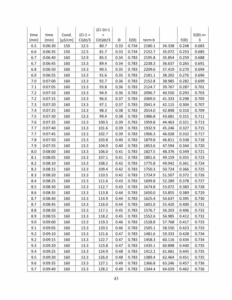
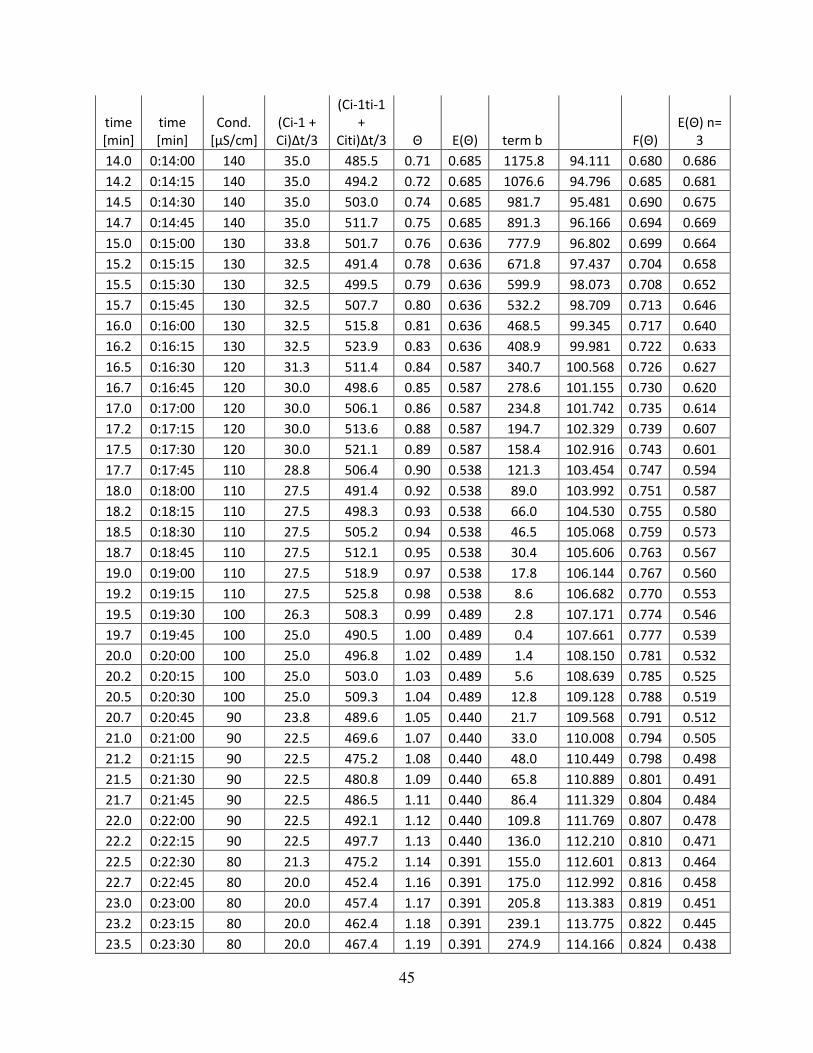
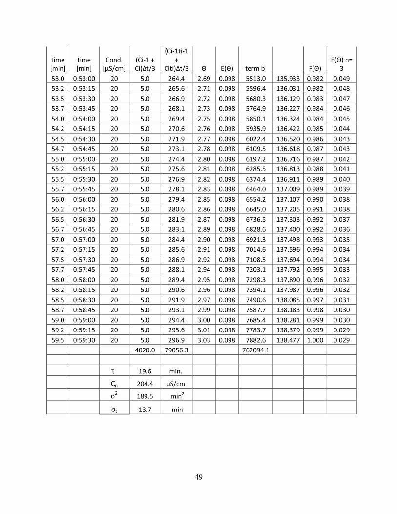
Table 8. E(Θ) and calculation for Brutus Water System and E(Θ) of two ideal CSTRs in series.

time [min]

Cond.

[μS/cm]

(Ci-1 +

Ci)Δt/3

(Ci-1ti-1

+

Citi)Δt/3 Θ E(Θ) term b F(Θ)

E(Θ) n=

3

0.0 0:00:00 0 0.00 0.000 0.000 0.000 0.000

0.1 0:00:05 0 0.0 0.0 0.00 0.000 0.0 0.000 0.000 0.017

0.2 0:00:10 0 0.0 0.0 0.01 0.000 0.0 0.000 0.000 0.033

0.2 0:00:15 0 0.0 0.0 0.01 0.000 0.0 0.000 0.000 0.050

0.3 0:00:20 0 0.0 0.0 0.02 0.000 0.0 0.000 0.000 0.066

0.4 0:00:25 0 0.0 0.0 0.02 0.000 0.0 0.000 0.000 0.081

0.5 0:00:30 0 0.0 0.0 0.03 0.000 0.0 0.000 0.000 0.097

0.6 0:00:35 0 0.0 0.0 0.03 0.000 0.0 0.000 0.000 0.112

0.7 0:00:40 0 0.0 0.0 0.03 0.000 0.0 0.000 0.000 0.127

0.7 0:00:45 10 0.4 0.3 0.04 0.049 149.0 0.049 0.000 0.141

0.8 0:00:50 10 0.8 0.7 0.04 0.049 296.7 0.098 0.001 0.156

0.9 0:00:55 10 0.8 0.7 0.05 0.049 294.1 0.147 0.001 0.170

1.0 0:01:00 10 0.8 0.8 0.05 0.049 291.5 0.196 0.001 0.184

1.1 0:01:05 10 0.8 0.9 0.06 0.049 288.9 0.245 0.002 0.197

1.2 0:01:10 30 1.7 1.9 0.06 0.147 571.4 0.391 0.003 0.211

1.2 0:01:15 40 2.9 3.5 0.06 0.196 992.5 0.587 0.004 0.224

1.3 0:01:20 40 3.3 4.3 0.07 0.196 1124.8 0.783 0.006 0.237

1.4 0:01:25 50 3.7 5.2 0.07 0.245 1253.4 1.027 0.007 0.249

1.5 0:01:30 50 4.2 6.1 0.08 0.245 1380.7 1.272 0.009 0.262

1.6 0:01:35 50 4.2 6.4 0.08 0.245 1368.1 1.516 0.011 0.274

1.7 0:01:40 60 4.6 7.5 0.08 0.293 1490.4 1.810 0.013 0.286

1.7 0:01:45 60 5.0 8.5 0.09 0.293 1611.6 2.103 0.015 0.298

1.8 0:01:50 60 5.0 9.0 0.09 0.293 1596.7 2.397 0.017 0.309

1.9 0:01:55 70 5.4 10.2 0.10 0.342 1713.1 2.739 0.020 0.321

2.0 0:02:00 70 5.8 11.4 0.10 0.342 1828.3 3.082 0.022 0.332

2.1 0:02:05 70 5.8 11.9 0.11 0.342 1811.1 3.424 0.025 0.343

2.2 0:02:10 80 6.2 13.3 0.11 0.391 1921.6 3.815 0.028 0.353

2.2 0:02:15 80 6.7 14.7 0.11 0.391 2030.9 4.207 0.030 0.364

2.3 0:02:20 80 6.7 15.3 0.12 0.391 2011.6 4.598 0.033 0.374

2.4 0:02:25 80 6.7 15.8 0.12 0.391 1992.3 4.989 0.036 0.384

2.5 0:02:30 80 6.7 16.4 0.13 0.391 1973.2 5.381 0.039 0.394

2.6 0:02:35 80 6.7 16.9 0.13 0.391 1954.1 5.772 0.042 0.404

2.7 0:02:40 80 6.7 17.5 0.14 0.391 1935.1 6.163 0.045 0.413

2.7 0:02:45 80 6.7 18.0 0.14 0.391 1916.3 6.555 0.047 0.423

2.8 0:02:50 90 7.1 19.8 0.14 0.440 2015.5 6.995 0.051 0.432

2.9 0:02:55 90 7.5 21.5 0.15 0.440 2113.7 7.435 0.054 0.441

3.0 0:03:00 100 7.9 23.4 0.15 0.489 2208.4 7.924 0.057 0.450

3.1 0:03:05 100 8.3 25.3 0.16 0.489 2302.1 8.413 0.061 0.458

42

time

[min]

time

[min]

Cond.

[μS/cm]

(Ci-1 +

Ci)Δt/3

(Ci-1ti-1

+

Citi)Δt/3 Θ E(Θ) term b F(Θ)

E(Θ) n=

3

3.2 0:03:15 100 8.3 26.7 0.17 0.489 2256.2 9.392 0.068 0.475

3.3 0:03:20 100 8.3 27.4 0.17 0.489 2233.4 9.881 0.071 0.483

3.4 0:03:25 100 8.3 28.1 0.17 0.489 2210.8 10.370 0.075 0.491

3.5 0:03:30 100 8.3 28.8 0.18 0.489 2188.2 10.859 0.078 0.499

3.6 0:03:35 100 8.3 29.5 0.18 0.489 2165.8 11.348 0.082 0.506

3.7 0:03:40 100 8.3 30.2 0.19 0.489 2143.5 11.837 0.085 0.514

3.7 0:03:45 100 8.3 30.9 0.19 0.489 2121.3 12.326 0.089 0.521

3.8 0:03:50 100 8.3 31.6 0.19 0.489 2099.2 12.816 0.093 0.528

3.9 0:03:55 100 8.3 32.3 0.20 0.489 2077.2 13.305 0.096 0.535

4.0 0:04:00 110 8.7 34.6 0.20 0.538 2157.6 13.843 0.100 0.542

4.1 0:04:05 110 9.2 37.0 0.21 0.538 2237.0 14.381 0.104 0.548

4.2 0:04:10 110 9.2 37.8 0.21 0.538 2213.2 14.919 0.108 0.555

4.2 0:04:15 120 9.6 40.3 0.22 0.587 2288.5 15.506 0.112 0.561

4.3 0:04:20 120 10.0 42.9 0.22 0.587 2362.9 16.093 0.116 0.567

4.4 0:04:25 120 10.0 43.7 0.22 0.587 2337.4 16.680 0.120 0.573

4.5 0:04:30 130 10.4 46.4 0.23 0.636 2407.8 17.316 0.125 0.579

4.6 0:04:35 130 10.8 49.2 0.23 0.636 2477.3 17.952 0.130 0.585

4.7 0:04:40 140 11.2 52.0 0.24 0.685 2543.8 18.636 0.135 0.590

4.7 0:04:45 140 11.7 54.9 0.24 0.685 2609.4 19.321 0.140 0.596

4.8 0:04:50 140 11.7 55.9 0.25 0.685 2580.4 20.006 0.144 0.601

4.9 0:04:55 140 11.7 56.8 0.25 0.685 2551.6 20.691 0.149 0.606

5.0 0:05:00 140 11.7 57.8 0.25 0.685 2522.9 21.376 0.154 0.612

5.1 0:05:05 140 11.7 58.8 0.26 0.685 2494.4 22.060 0.159 0.616

5.2 0:05:10 140 11.7 59.7 0.26 0.685 2466.1 22.745 0.164 0.621

5.2 0:05:15 140 11.7 60.7 0.27 0.685 2437.9 23.430 0.169 0.626

5.3 0:05:20 140 11.7 61.7 0.27 0.685 2409.9 24.115 0.174 0.631

5.4 0:05:25 140 11.7 62.7 0.28 0.685 2382.1 24.800 0.179 0.635

5.5 0:05:30 150 12.1 65.9 0.28 0.734 2438.0 25.533 0.184 0.639

5.6 0:05:35 150 12.5 69.2 0.28 0.734 2493.0 26.267 0.190 0.644

5.7 0:05:40 150 12.5 70.3 0.29 0.734 2463.7 27.001 0.195 0.648

5.7 0:05:45 150 12.5 71.3 0.29 0.734 2434.6 27.734 0.200 0.652

5.8 0:05:50 150 12.5 72.3 0.30 0.734 2405.6 28.468 0.206 0.655

5.9 0:05:55 150 12.5 73.4 0.30 0.734 2376.8 29.202 0.211 0.659

6.0 0:06:00 150 12.5 74.4 0.30 0.734 2348.2 29.936 0.216 0.663

6.1 0:06:05 150 12.5 75.5 0.31 0.734 2319.7 30.669 0.221 0.666

6.2 0:06:10 150 12.5 76.5 0.31 0.734 2291.5 31.403 0.227 0.670

6.2 0:06:15 150 12.5 77.5 0.32 0.734 2263.4 32.137 0.232 0.673

6.3 0:06:20 150 12.5 78.6 0.32 0.734 2235.4 32.870 0.237 0.676

6.4 0:06:25 150 12.5 79.6 0.33 0.734 2207.7 33.604 0.243 0.680

43

time

[min]

time

[min]

Cond.

[μS/cm]

(Ci-1 +

Ci)Δt/3

(Ci-1ti-1

+

Citi)Δt/3 Θ E(Θ) term b F(Θ)

E(Θ) n=

3

6.5 0:06:30 150 12.5 80.7 0.33 0.734 2180.1 34.338 0.248 0.683

6.6 0:06:35 150 12.5 81.7 0.33 0.734 2152.7 35.072 0.253 0.685

6.7 0:06:40 160 12.9 85.5 0.34 0.783 2195.8 35.854 0.259 0.688

6.7 0:06:45 160 13.3 89.4 0.34 0.783 2238.3 36.637 0.265 0.691

6.8 0:06:50 160 13.3 90.5 0.35 0.783 2209.6 37.419 0.270 0.694

6.9 0:06:55 160 13.3 91.6 0.35 0.783 2181.1 38.202 0.276 0.696

7.0 0:07:00 160 13.3 92.7 0.36 0.783 2152.8 38.985 0.282 0.699

7.1 0:07:05 160 13.3 93.8 0.36 0.783 2124.7 39.767 0.287 0.701

7.2 0:07:10 160 13.3 94.9 0.36 0.783 2096.7 40.550 0.293 0.703

7.2 0:07:15 160 13.3 96.0 0.37 0.783 2069.0 41.333 0.298 0.705

7.3 0:07:20 160 13.3 97.1 0.37 0.783 2041.4 42.115 0.304 0.707

7.4 0:07:25 160 13.3 98.3 0.38 0.783 2014.0 42.898 0.310 0.709

7.5 0:07:30 160 13.3 99.4 0.38 0.783 1986.8 43.681 0.315 0.711

7.6 0:07:35 160 13.3 100.5 0.39 0.783 1959.8 44.463 0.321 0.713

7.7 0:07:40 160 13.3 101.6 0.39 0.783 1932.9 45.246 0.327 0.715

7.7 0:07:45 160 13.3 102.7 0.39 0.783 1906.3 46.028 0.332 0.717

7.8 0:07:50 160 13.3 103.8 0.40 0.783 1879.8 46.811 0.338 0.718

7.9 0:07:55 160 13.3 104.9 0.40 0.783 1853.6 47.594 0.344 0.720

8.0 0:08:00 160 13.3 106.0 0.41 0.783 1827.5 48.376 0.349 0.721

8.1 0:08:05 160 13.3 107.1 0.41 0.783 1801.6 49.159 0.355 0.723

8.2 0:08:10 160 13.3 108.2 0.42 0.783 1775.8 49.942 0.361 0.724

8.2 0:08:15 160 13.3 109.4 0.42 0.783 1750.3 50.724 0.366 0.725

8.3 0:08:20 160 13.3 110.5 0.42 0.783 1724.9 51.507 0.372 0.726

8.4 0:08:25 160 13.3 111.6 0.43 0.783 1699.8 52.289 0.378 0.727

8.5 0:08:30 160 13.3 112.7 0.43 0.783 1674.8 53.072 0.383 0.728

8.6 0:08:35 160 13.3 113.8 0.44 0.783 1650.0 53.855 0.389 0.729

8.7 0:08:40 160 13.3 114.9 0.44 0.783 1625.4 54.637 0.395 0.730

8.7 0:08:45 160 13.3 116.0 0.44 0.783 1601.0 55.420 0.400 0.731

8.8 0:08:50 160 13.3 117.1 0.45 0.783 1576.7 56.203 0.406 0.732

8.9 0:08:55 160 13.3 118.2 0.45 0.783 1552.6 56.985 0.412 0.732

9.0 0:09:00 160 13.3 119.3 0.46 0.783 1528.8 57.768 0.417 0.733

9.1 0:09:05 160 13.3 120.5 0.46 0.783 1505.1 58.550 0.423 0.733

9.2 0:09:10 160 13.3 121.6 0.47 0.783 1481.6 59.333 0.428 0.734

9.2 0:09:15 160 13.3 122.7 0.47 0.783 1458.3 60.116 0.434 0.734

9.3 0:09:20 160 13.3 123.8 0.47 0.783 1435.1 60.898 0.440 0.735

9.4 0:09:25 160 13.3 124.9 0.48 0.783 1412.2 61.681 0.445 0.735

9.5 0:09:30 160 13.3 126.0 0.48 0.783 1389.4 62.464 0.451 0.735

9.6 0:09:35 160 13.3 127.1 0.49 0.783 1366.8 63.246 0.457 0.736

9.7 0:09:40 160 13.3 128.2 0.49 0.783 1344.4 64.029 0.462 0.736

44

time

[min]

time

[min]

Cond.

[μS/cm]

(Ci-1 +

Ci)Δt/3

(Ci-1ti-1

+

Citi)Δt/3 Θ E(Θ) term b F(Θ)

E(Θ) n=

3

9.7 0:09:45 160 13.3 129.3 0.50 0.783 1322.2 64.812 0.468 0.736

9.8 0:09:50 160 13.3 130.5 0.50 0.783 1300.2 65.594 0.474 0.736

9.9 0:09:55 160 13.3 131.6 0.50 0.783 1278.4 66.377 0.479 0.736

10.0 0:10:00 160 13.3 132.7 0.51 0.783 1256.7 67.159 0.485 0.736

10.1 0:10:05 160 13.3 133.8 0.51 0.783 1235.3 67.942 0.491 0.736

10.2 0:10:10 160 13.3 134.9 0.52 0.783 1214.0 68.725 0.496 0.735

10.2 0:10:15 160 13.3 136.0 0.52 0.783 1192.9 69.507 0.502 0.735

10.3 0:10:20 160 13.3 137.1 0.53 0.783 1172.0 70.290 0.508 0.735

10.4 0:10:25 160 13.3 138.2 0.53 0.783 1151.2 71.073 0.513 0.735

10.5 0:10:30 160 13.3 139.3 0.53 0.783 1130.7 71.855 0.519 0.734

10.6 0:10:35 160 13.3 140.4 0.54 0.783 1110.3 72.638 0.525 0.734

10.7 0:10:40 160 13.3 141.6 0.54 0.783 1090.2 73.420 0.530 0.733

10.7 0:10:45 160 13.3 142.7 0.55 0.783 1070.2 74.203 0.536 0.733

10.8 0:10:50 160 13.3 143.8 0.55 0.783 1050.4 74.986 0.542 0.732

10.9 0:10:55 160 13.3 144.9 0.55 0.783 1030.7 75.768 0.547 0.732

11.0 0:11:00 160 13.3 146.0 0.56 0.783 1011.3 76.551 0.553 0.731

11.1 0:11:05 160 13.3 147.1 0.56 0.783 992.1 77.334 0.558 0.730

11.2 0:11:10 160 13.3 148.2 0.57 0.783 973.0 78.116 0.564 0.730

11.2 0:11:15 150 12.9 144.6 0.57 0.734 924.6 78.850 0.569 0.729

11.3 0:11:20 150 12.5 141.0 0.58 0.734 877.0 79.584 0.575 0.728

11.4 0:11:25 150 12.5 142.1 0.58 0.734 859.6 80.317 0.580 0.727

11.5 0:11:30 150 12.5 143.1 0.58 0.734 842.4 81.051 0.585 0.726

11.6 0:11:35 150 12.5 144.2 0.59 0.734 825.4 81.785 0.591 0.725

11.7 0:11:40 150 12.5 145.2 0.59 0.734 808.6 82.519 0.596 0.724

11.7 0:11:45 150 12.5 146.2 0.60 0.734 791.9 83.252 0.601 0.724

11.8 0:11:50 150 12.5 147.3 0.60 0.734 775.4 83.986 0.606 0.722

11.9 0:11:55 150 12.5 148.3 0.61 0.734 759.1 84.720 0.612 0.721

12.0 0:12:00 150 12.5 149.4 0.61 0.734 743.0 85.453 0.617 0.720

12.1 0:12:05 150 12.5 150.4 0.61 0.734 727.0 86.187 0.622 0.719

12.2 0:12:10 150 12.5 151.4 0.62 0.734 711.2 86.921 0.628 0.718

12.2 0:12:15 150 12.5 152.5 0.62 0.734 695.6 87.655 0.633 0.717

12.3 0:12:20 150 12.5 153.5 0.63 0.734 680.2 88.388 0.638 0.716

12.4 0:12:25 150 12.5 154.6 0.63 0.734 664.9 89.122 0.644 0.714

12.5 0:12:30 150 12.5 155.6 0.64 0.734 649.8 89.856 0.649 0.713

12.7 0:12:45 150 37.5 473.3 0.65 0.734 1861.6 90.589 0.654 0.709

13.0 0:13:00 150 37.5 482.6 0.66 0.734 1731.9 91.323 0.659 0.705

13.2 0:13:15 150 37.5 492.0 0.67 0.734 1606.8 92.057 0.665 0.700

13.5 0:13:30 140 36.3 484.5 0.69 0.685 1438.9 92.742 0.670 0.696

13.7 0:13:45 140 35.0 476.7 0.70 0.685 1279.4 93.426 0.675 0.691

45

time

[min]

time

[min]

Cond.

[μS/cm]

(Ci-1 +

Ci)Δt/3

(Ci-1ti-1

+

Citi)Δt/3 Θ E(Θ) term b F(Θ)

E(Θ) n=

3

14.0 0:14:00 140 35.0 485.5 0.71 0.685 1175.8 94.111 0.680 0.686

14.2 0:14:15 140 35.0 494.2 0.72 0.685 1076.6 94.796 0.685 0.681

14.5 0:14:30 140 35.0 503.0 0.74 0.685 981.7 95.481 0.690 0.675

14.7 0:14:45 140 35.0 511.7 0.75 0.685 891.3 96.166 0.694 0.669

15.0 0:15:00 130 33.8 501.7 0.76 0.636 777.9 96.802 0.699 0.664

15.2 0:15:15 130 32.5 491.4 0.78 0.636 671.8 97.437 0.704 0.658

15.5 0:15:30 130 32.5 499.5 0.79 0.636 599.9 98.073 0.708 0.652

15.7 0:15:45 130 32.5 507.7 0.80 0.636 532.2 98.709 0.713 0.646

16.0 0:16:00 130 32.5 515.8 0.81 0.636 468.5 99.345 0.717 0.640

16.2 0:16:15 130 32.5 523.9 0.83 0.636 408.9 99.981 0.722 0.633

16.5 0:16:30 120 31.3 511.4 0.84 0.587 340.7 100.568 0.726 0.627

16.7 0:16:45 120 30.0 498.6 0.85 0.587 278.6 101.155 0.730 0.620

17.0 0:17:00 120 30.0 506.1 0.86 0.587 234.8 101.742 0.735 0.614

17.2 0:17:15 120 30.0 513.6 0.88 0.587 194.7 102.329 0.739 0.607

17.5 0:17:30 120 30.0 521.1 0.89 0.587 158.4 102.916 0.743 0.601

17.7 0:17:45 110 28.8 506.4 0.90 0.538 121.3 103.454 0.747 0.594

18.0 0:18:00 110 27.5 491.4 0.92 0.538 89.0 103.992 0.751 0.587

18.2 0:18:15 110 27.5 498.3 0.93 0.538 66.0 104.530 0.755 0.580

18.5 0:18:30 110 27.5 505.2 0.94 0.538 46.5 105.068 0.759 0.573

18.7 0:18:45 110 27.5 512.1 0.95 0.538 30.4 105.606 0.763 0.567

19.0 0:19:00 110 27.5 518.9 0.97 0.538 17.8 106.144 0.767 0.560

19.2 0:19:15 110 27.5 525.8 0.98 0.538 8.6 106.682 0.770 0.553

19.5 0:19:30 100 26.3 508.3 0.99 0.489 2.8 107.171 0.774 0.546

19.7 0:19:45 100 25.0 490.5 1.00 0.489 0.4 107.661 0.777 0.539

20.0 0:20:00 100 25.0 496.8 1.02 0.489 1.4 108.150 0.781 0.532

20.2 0:20:15 100 25.0 503.0 1.03 0.489 5.6 108.639 0.785 0.525

20.5 0:20:30 100 25.0 509.3 1.04 0.489 12.8 109.128 0.788 0.519

20.7 0:20:45 90 23.8 489.6 1.05 0.440 21.7 109.568 0.791 0.512

21.0 0:21:00 90 22.5 469.6 1.07 0.440 33.0 110.008 0.794 0.505

21.2 0:21:15 90 22.5 475.2 1.08 0.440 48.0 110.449 0.798 0.498

21.5 0:21:30 90 22.5 480.8 1.09 0.440 65.8 110.889 0.801 0.491

21.7 0:21:45 90 22.5 486.5 1.11 0.440 86.4 111.329 0.804 0.484

22.0 0:22:00 90 22.5 492.1 1.12 0.440 109.8 111.769 0.807 0.478

22.2 0:22:15 90 22.5 497.7 1.13 0.440 136.0 112.210 0.810 0.471

22.5 0:22:30 80 21.3 475.2 1.14 0.391 155.0 112.601 0.813 0.464

22.7 0:22:45 80 20.0 452.4 1.16 0.391 175.0 112.992 0.816 0.458

23.0 0:23:00 80 20.0 457.4 1.17 0.391 205.8 113.383 0.819 0.451

23.2 0:23:15 80 20.0 462.4 1.18 0.391 239.1 113.775 0.822 0.445

23.5 0:23:30 80 20.0 467.4 1.19 0.391 274.9 114.166 0.824 0.438

46

time

[min]

time

[min]

Cond.

[μS/cm]

(Ci-1 +

Ci)Δt/3

(Ci-1ti-1

+

Citi)Δt/3 Θ E(Θ) term b F(Θ)

E(Θ) n=

3

23.7 0:23:45 80 20.0 472.4 1.21 0.391 313.2 114.557 0.827 0.432

24.0 0:24:00 80 20.0 477.4 1.22 0.391 354.0 114.949 0.830 0.425

24.2 0:24:15 80 20.0 482.4 1.23 0.391 397.3 115.340 0.833 0.419

24.5 0:24:30 80 20.0 487.4 1.25 0.391 443.1 115.731 0.836 0.413

24.7 0:24:45 70 18.8 461.5 1.26 0.342 459.2 116.074 0.838 0.406

25.0 0:25:00 70 17.5 435.2 1.27 0.342 474.4 116.416 0.841 0.400

25.2 0:25:15 70 17.5 439.6 1.28 0.342 521.1 116.759 0.843 0.394

25.5 0:25:30 70 17.5 444.0 1.30 0.342 569.9 117.101 0.846 0.388

25.7 0:25:45 70 17.5 448.4 1.31 0.342 620.9 117.443 0.848 0.382

26.0 0:26:00 70 17.5 452.7 1.32 0.342 674.1 117.786 0.851 0.376

26.2 0:26:15 70 17.5 457.1 1.33 0.342 729.5 118.128 0.853 0.370

26.5 0:26:30 60 16.3 428.4 1.35 0.293 728.8 118.422 0.855 0.364

26.7 0:26:45 60 15.0 399.3 1.36 0.293 725.9 118.715 0.857 0.358

27.0 0:27:00 60 15.0 403.1 1.37 0.293 779.0 119.009 0.859 0.353

27.2 0:27:15 60 15.0 406.8 1.39 0.293 834.0 119.302 0.862 0.347

27.5 0:27:30 60 15.0 410.6 1.40 0.293 890.8 119.596 0.864 0.341

27.7 0:27:45 60 15.0 414.3 1.41 0.293 949.5 119.889 0.866 0.336

28.0 0:28:00 60 15.0 418.1 1.42 0.293 1010.1 120.183 0.868 0.330

28.2 0:28:15 60 15.0 421.8 1.44 0.293 1072.6 120.476 0.870 0.325

28.5 0:28:30 60 15.0 425.6 1.45 0.293 1137.0 120.770 0.872 0.320

28.7 0:28:45 60 15.0 429.3 1.46 0.293 1203.2 121.063 0.874 0.314

29.0 0:29:00 60 15.0 433.1 1.47 0.293 1271.3 121.357 0.876 0.309

29.2 0:29:15 60 15.0 436.8 1.49 0.293 1341.3 121.650 0.878 0.304

29.5 0:29:30 50 13.8 403.7 1.50 0.245 1292.3 121.895 0.880 0.299

29.7 0:29:45 50 12.5 370.3 1.51 0.245 1239.1 122.139 0.882 0.294

30.0 0:30:00 50 12.5 373.4 1.53 0.245 1302.1 122.384 0.884 0.289

30.2 0:30:15 50 12.5 376.5 1.54 0.245 1366.6 122.628 0.886 0.284

30.5 0:30:30 50 12.5 379.6 1.55 0.245 1432.7 122.873 0.887 0.279

30.7 0:30:45 50 12.5 382.8 1.56 0.245 1500.4 123.117 0.889 0.274

31.0 0:31:00 50 12.5 385.9 1.58 0.245 1569.7 123.362 0.891 0.270

31.2 0:31:15 50 12.5 389.0 1.59 0.245 1640.5 123.607 0.893 0.265

31.5 0:31:30 50 12.5 392.1 1.60 0.245 1712.9 123.851 0.894 0.260

31.7 0:31:45 50 12.5 395.3 1.61 0.245 1786.8 124.096 0.896 0.256

32.0 0:32:00 50 12.5 398.4 1.63 0.245 1862.3 124.340 0.898 0.251

32.2 0:32:15 40 11.2 361.2 1.64 0.196 1741.6 124.536 0.899 0.247

32.5 0:32:30 40 10.0 323.7 1.65 0.196 1614.4 124.732 0.901 0.243

32.7 0:32:45 40 10.0 326.2 1.67 0.196 1678.6 124.927 0.902 0.238

33.0 0:33:00 40 10.0 328.7 1.68 0.196 1744.0 125.123 0.904 0.234

33.2 0:33:15 40 10.0 331.2 1.69 0.196 1810.6 125.319 0.905 0.230

47

time

[min]

time

[min]

Cond.

[μS/cm]

(Ci-1 +

Ci)Δt/3

(Ci-1ti-1

+

Citi)Δt/3 Θ E(Θ) term b F(Θ)

E(Θ) n=

3

33.5 0:33:30 40 10.0 333.7 1.70 0.196 1878.5 125.514 0.906 0.226

33.7 0:33:45 40 10.0 336.2 1.72 0.196 1947.7 125.710 0.908 0.222

34.0 0:34:00 40 10.0 338.7 1.73 0.196 2018.1 125.906 0.909 0.218

34.2 0:34:15 40 10.0 341.2 1.74 0.196 2089.7 126.101 0.911 0.214

34.5 0:34:30 40 10.0 343.7 1.75 0.196 2162.6 126.297 0.912 0.210

34.7 0:34:45 40 10.0 346.2 1.77 0.196 2236.8 126.493 0.913 0.206

35.0 0:35:00 40 10.0 348.7 1.78 0.196 2312.2 126.688 0.915 0.203

35.2 0:35:15 40 10.0 351.2 1.79 0.196 2388.8 126.884 0.916 0.199

35.5 0:35:30 40 10.0 353.7 1.81 0.196 2466.7 127.080 0.918 0.195

35.7 0:35:45 30 8.8 311.5 1.82 0.147 2222.7 127.226 0.919 0.192

36.0 0:36:00 30 7.5 269.0 1.83 0.147 1969.7 127.373 0.920 0.188

36.2 0:36:15 30 7.5 270.9 1.84 0.147 2031.0 127.520 0.921 0.185

36.5 0:36:30 30 7.5 272.8 1.86 0.147 2093.1 127.666 0.922 0.181

36.7 0:36:45 30 7.5 274.7 1.87 0.147 2156.2 127.813 0.923 0.178

37.0 0:37:00 30 7.5 276.5 1.88 0.147 2220.3 127.960 0.924 0.175

37.2 0:37:15 30 7.5 278.4 1.89 0.147 2285.3 128.107 0.925 0.172

37.5 0:37:30 30 7.5 280.3 1.91 0.147 2351.2 128.253 0.926 0.168

37.7 0:37:45 30 7.5 282.2 1.92 0.147 2418.1 128.400 0.927 0.165

38.0 0:38:00 30 7.5 284.0 1.93 0.147 2485.9 128.547 0.928 0.162

38.2 0:38:15 30 7.5 285.9 1.94 0.147 2554.6 128.694 0.929 0.159

38.5 0:38:30 30 7.5 287.8 1.96 0.147 2624.3 128.840 0.930 0.156

38.7 0:38:45 30 7.5 289.7 1.97 0.147 2694.9 128.987 0.931 0.153

39.0 0:39:00 30 7.5 291.5 1.98 0.147 2766.5 129.134 0.933 0.150

39.2 0:39:15 30 7.5 293.4 2.00 0.147 2838.9 129.281 0.934 0.147

39.5 0:39:30 30 7.5 295.3 2.01 0.147 2912.4 129.427 0.935 0.145

39.7 0:39:45 30 7.5 297.2 2.02 0.147 2986.7 129.574 0.936 0.142

40.0 0:40:00 30 7.5 299.0 2.03 0.147 3062.0 129.721 0.937 0.139

40.2 0:40:15 30 7.5 300.9 2.05 0.147 3138.3 129.868 0.938 0.137

40.5 0:40:30 30 7.5 302.8 2.06 0.147 3215.4 130.014 0.939 0.134

40.7 0:40:45 30 7.5 304.7 2.07 0.147 3293.6 130.161 0.940 0.131

41.0 0:41:00 30 7.5 306.5 2.08 0.147 3372.6 130.308 0.941 0.129

41.2 0:41:15 30 7.5 308.4 2.10 0.147 3452.6 130.455 0.942 0.126

41.5 0:41:30 30 7.5 310.3 2.11 0.147 3533.5 130.601 0.943 0.124

41.7 0:41:45 30 7.5 312.2 2.12 0.147 3615.4 130.748 0.944 0.122

42.0 0:42:00 30 7.5 314.0 2.14 0.147 3698.2 130.895 0.945 0.119

42.2 0:42:15 30 7.5 315.9 2.15 0.147 3781.9 131.042 0.946 0.117

42.5 0:42:30 30 7.5 317.8 2.16 0.147 3866.6 131.188 0.947 0.115

42.7 0:42:45 30 7.5 319.7 2.17 0.147 3952.2 131.335 0.948 0.113

43.0 0:43:00 30 7.5 321.5 2.19 0.147 4038.8 131.482 0.949 0.110

48

time

[min]

time

[min]

Cond.

[μS/cm]

(Ci-1 +

Ci)Δt/3

(Ci-1ti-1

+

Citi)Δt/3 Θ E(Θ) term b F(Θ)

E(Θ) n=

3

43.2 0:43:15 30 7.5 323.4 2.20 0.147 4126.3 131.629 0.951 0.108

43.5 0:43:30 30 7.5 325.3 2.21 0.147 4214.7 131.775 0.952 0.106

43.7 0:43:45 30 7.5 327.2 2.22 0.147 4304.1 131.922 0.953 0.104

44.0 0:44:00 30 7.5 329.0 2.24 0.147 4394.4 132.069 0.954 0.102

44.2 0:44:15 30 7.5 330.9 2.25 0.147 4485.6 132.216 0.955 0.100

44.5 0:44:30 30 7.5 332.8 2.26 0.147 4577.8 132.362 0.956 0.098

44.7 0:44:45 30 7.5 334.7 2.28 0.147 4670.9 132.509 0.957 0.096

45.0 0:45:00 30 7.5 336.5 2.29 0.147 4764.9 132.656 0.958 0.094

45.2 0:45:15 30 7.5 338.4 2.30 0.147 4859.9 132.802 0.959 0.092

45.5 0:45:30 30 7.5 340.3 2.31 0.147 4955.8 132.949 0.960 0.091

45.7 0:45:45 30 7.5 342.2 2.33 0.147 5052.7 133.096 0.961 0.089

46.0 0:46:00 20 6.3 286.5 2.34 0.098 4283.9 133.194 0.962 0.087

46.2 0:46:15 20 5.0 230.6 2.35 0.098 3499.5 133.292 0.963 0.085

46.5 0:46:30 20 5.0 231.9 2.36 0.098 3566.0 133.389 0.963 0.084

46.7 0:46:45 20 5.0 233.1 2.38 0.098 3633.0 133.487 0.964 0.082

47.0 0:47:00 20 5.0 234.4 2.39 0.098 3700.7 133.585 0.965 0.080

47.2 0:47:15 20 5.0 235.6 2.40 0.098 3769.1 133.683 0.965 0.079

47.5 0:47:30 20 5.0 236.9 2.42 0.098 3838.0 133.781 0.966 0.077

47.7 0:47:45 20 5.0 238.1 2.43 0.098 3907.6 133.879 0.967 0.076

48.0 0:48:00 20 5.0 239.4 2.44 0.098 3977.8 133.976 0.968 0.074

48.2 0:48:15 20 5.0 240.6 2.45 0.098 4048.6 134.074 0.968 0.073

48.5 0:48:30 20 5.0 241.9 2.47 0.098 4120.1 134.172 0.969 0.071

48.7 0:48:45 20 5.0 243.1 2.48 0.098 4192.1 134.270 0.970 0.070

49.0 0:49:00 20 5.0 244.4 2.49 0.098 4264.8 134.368 0.970 0.068

49.2 0:49:15 20 5.0 245.6 2.50 0.098 4338.2 134.466 0.971 0.067

49.5 0:49:30 20 5.0 246.9 2.52 0.098 4412.1 134.563 0.972 0.066

49.7 0:49:45 20 5.0 248.1 2.53 0.098 4486.7 134.661 0.972 0.064

50.0 0:50:00 20 5.0 249.4 2.54 0.098 4561.9 134.759 0.973 0.063

50.2 0:50:15 20 5.0 250.6 2.56 0.098 4637.7 134.857 0.974 0.062

50.5 0:50:30 20 5.0 251.9 2.57 0.098 4714.2 134.955 0.975 0.060

50.7 0:50:45 20 5.0 253.1 2.58 0.098 4791.2 135.053 0.975 0.059

51.0 0:51:00 20 5.0 254.4 2.59 0.098 4868.9 135.150 0.976 0.058

51.2 0:51:15 20 5.0 255.6 2.61 0.098 4947.3 135.248 0.977 0.057

51.5 0:51:30 20 5.0 256.9 2.62 0.098 5026.2 135.346 0.977 0.056

51.7 0:51:45 20 5.0 258.1 2.63 0.098 5105.8 135.444 0.978 0.055

52.0 0:52:00 20 5.0 259.4 2.64 0.098 5186.0 135.542 0.979 0.053

52.2 0:52:15 20 5.0 260.6 2.66 0.098 5266.8 135.640 0.980 0.052

52.5 0:52:30 20 5.0 261.9 2.67 0.098 5348.3 135.737 0.980 0.051

52.7 0:52:45 20 5.0 263.1 2.68 0.098 5430.3 135.835 0.981 0.050

49

time

[min]

time

[min]

Cond.

[μS/cm]

(Ci-1 +

Ci)Δt/3

(Ci-1ti-1

+

Citi)Δt/3 Θ E(Θ) term b F(Θ)

E(Θ) n=

3

53.0 0:53:00 20 5.0 264.4 2.69 0.098 5513.0 135.933 0.982 0.049

53.2 0:53:15 20 5.0 265.6 2.71 0.098 5596.4 136.031 0.982 0.048

53.5 0:53:30 20 5.0 266.9 2.72 0.098 5680.3 136.129 0.983 0.047

53.7 0:53:45 20 5.0 268.1 2.73 0.098 5764.9 136.227 0.984 0.046

54.0 0:54:00 20 5.0 269.4 2.75 0.098 5850.1 136.324 0.984 0.045

54.2 0:54:15 20 5.0 270.6 2.76 0.098 5935.9 136.422 0.985 0.044

54.5 0:54:30 20 5.0 271.9 2.77 0.098 6022.4 136.520 0.986 0.043

54.7 0:54:45 20 5.0 273.1 2.78 0.098 6109.5 136.618 0.987 0.043

55.0 0:55:00 20 5.0 274.4 2.80 0.098 6197.2 136.716 0.987 0.042

55.2 0:55:15 20 5.0 275.6 2.81 0.098 6285.5 136.813 0.988 0.041

55.5 0:55:30 20 5.0 276.9 2.82 0.098 6374.4 136.911 0.989 0.040

55.7 0:55:45 20 5.0 278.1 2.83 0.098 6464.0 137.009 0.989 0.039

56.0 0:56:00 20 5.0 279.4 2.85 0.098 6554.2 137.107 0.990 0.038

56.2 0:56:15 20 5.0 280.6 2.86 0.098 6645.0 137.205 0.991 0.038

56.5 0:56:30 20 5.0 281.9 2.87 0.098 6736.5 137.303 0.992 0.037

56.7 0:56:45 20 5.0 283.1 2.89 0.098 6828.6 137.400 0.992 0.036

57.0 0:57:00 20 5.0 284.4 2.90 0.098 6921.3 137.498 0.993 0.035

57.2 0:57:15 20 5.0 285.6 2.91 0.098 7014.6 137.596 0.994 0.034

57.5 0:57:30 20 5.0 286.9 2.92 0.098 7108.5 137.694 0.994 0.034

57.7 0:57:45 20 5.0 288.1 2.94 0.098 7203.1 137.792 0.995 0.033

58.0 0:58:00 20 5.0 289.4 2.95 0.098 7298.3 137.890 0.996 0.032

58.2 0:58:15 20 5.0 290.6 2.96 0.098 7394.1 137.987 0.996 0.032

58.5 0:58:30 20 5.0 291.9 2.97 0.098 7490.6 138.085 0.997 0.031

58.7 0:58:45 20 5.0 293.1 2.99 0.098 7587.7 138.183 0.998 0.030

59.0 0:59:00 20 5.0 294.4 3.00 0.098 7685.4 138.281 0.999 0.030

59.2 0:59:15 20 5.0 295.6 3.01 0.098 7783.7 138.379 0.999 0.029

59.5 0:59:30 20 5.0 296.9 3.03 0.098 7882.6 138.477 1.000 0.029

4020.0 79056.3 762094.1

t 19.6 min.

Cn 204.4 uS/cm

σ2 189.5 min

2

σt 13.7 min