The Impact of Signal Bandwidth on Indoor Wireless Systems in Dense Multipath Environments Daniel J. Hibbard Thesis submitted to the Faculty of the Virginia Polytechnic Institute and State University in partial fulfillment of the requirements for the degree of MASTER OF SCIENCE In Electrical Engineering Dr. R. Michael Buehrer, Chair Dr. William A. Davis Dr. Jeffery Reed May 13, 2004 Blacksburg, Virginia Keywords: Spreading Bandwidth, Propagation Measurements, Sliding Correlator, Rake Receiver, Channel Estimation, Channel Characterization, CDMA Copyright 2004, Daniel J. Hibbard
Transcript
The Impact of Signal Bandwidth on Indoor Wireless Systems in Dense Multipath Environments
Daniel J. Hibbard
Thesis submitted to the Faculty of the Virginia Polytechnic Institute and State University in partial fulfillment of the requirements for the degree of
MASTER OF SCIENCE In
Electrical Engineering
Dr. R. Michael Buehrer, Chair Dr. William A. Davis
The Impact of Signal Bandwidth on Indoor Wireless Systems in Dense Multipath Environments
Daniel J. Hibbard
Abstract
Recently there has been a significant amount of interest in the area of wideband and ultra-wideband (UWB) signaling for use in indoor wireless systems. This interest is in part motivated by the notion that the use of large bandwidth signals makes systems less sensitive to the degrading effects of multipath propagation. By reducing the sensitivity to multipath, more robust and higher capacity systems can be realized. However, as signal bandwidth is increased, the complexity of a Rake receiver (or other receiver structure) required to capture the available power also increases. In addition, accurate channel estimation is required to realize this performance, which becomes increasingly difficult as energy is dispersed among more multipath components. In this thesis we quantify the channel response for six signal bandwidths ranging from continuous wave (CW) to 1 GHz transmission bandwidths. We present large scale and small scale fading statistics for both LOS and NLOS indoor channels based on an indoor measurement campaign conducted in Durham Hall at Virginia Tech. Using newly developed antenna positioning equipment we also quantify the spatial correlation of these signals. It is shown that the incremental performance gains due to reduced fading of large bandwidths level off as signals approach UWB bandwidths. Furthermore, we analyze the performance of Rake receivers for the different signal bandwidths and compare their performance for binary phase modulation (BPSK). It is shown that the receiver structure and performance is critical in realizing the reduced fading benefit of large signal bandwidths. We show practical channel estimation degrades performance more for larger bandwidths. We also demonstrate for a fixed finger Rake receiver there is an optimal signal bandwidth beyond which increased signal bandwidth produces degrading results.
iii
For Ashley, who was there every step of the way
iv
Acknowledgments At this time I would like to thank Michael Buehrer, William Davis, Jeffery Reed, and Raqib Mostafa for serving on my advisory committee and providing technical expertise as well as encouragement along the way. I would also like to acknowledge the Via family for the generous endowment provided by the Harry Lynde Bradley Fellowship which allowed me to pursue this research almost completely un-tethered from the reins. I would also like to express my appreciation to my fellow graduate students in MPRG, especailly Joseph Gaeddert, Chris Anderson, Brian Donlan, Vivek Bharadwaj, Aaron Orndorf and John Keaveny for their thought provoking discussions and technical assistance with this research. Also my appreciation goes to Samir Ginde, Carlos Aguayo, Nathan Harter and my other lab mates for keeping things in perspective while working at MPRG. Of the MPRG staff, which was extremely helpful, I would like to thank Mike Hill, Shelby Smith, Hilda Reynolds, and Shereef Sayed. I am greatly indebted to Mike Coyle and the staff of the Industrial Design Metal Shop for their help in designing and manufacturing the antenna positioning system. Without Mike’s support the positioning system would not have proceeded beyond the conceptual stage. For donating replacement couplers for the positioning system I would like to thank the staff at Ruland. I also owe thanks to Josiah Hernandez for helping with the measurement campaign. I must also thank Dennis Sweeney from CWT and Carl Dietrich from VTAG for their insight and use of their equipment during the measurement campaign. I owe a very special thanks to Alexander Taylor, who has been my partner in Electrical Engineering crime for the past five years at Virginia Tech and has been an honest friend through it all. Also the friendships forged with Aaron Orndorf and Jeremy Barry have made this experience an interesting one to say the least. Without a doubt none of this work would have been possible without the tireless support and understanding of my fiancé and soon to be wife Ashley K. Rentz. Her encouragement, wisdom, and unwavering love were instrumental in completing this work; thank you for understanding. Finally, I would like to thank my parents Bob and Louise Hibbard, as well as my brother Mark Hibbard for their generous support, love, and understanding throughout this work as well as my entire life. Dan Hibbard May 20, 2004
v
Table of Contents
CHAPTER 1
INTRODUCTION AND THESIS OVERVIEW .......................................................1
RADIO WAVE PROPAGATION AND THE INDOOR PROPAGATION CHANNEL ............................................................................................................5
2.2 Propagation Overview ................................................................................................................... 6 2.2.1 Antennas and Radiation............................................................................................................... 6 2.2.2 Propagation Mechanisms............................................................................................................. 9 2.2.3 The Friis Transmission Formula and Basic Communication Link ............................................ 14
2.3 The Indoor Propagation Channel ............................................................................................... 17 2.3.1 Large Scale Effects.................................................................................................................... 17 2.3.2 Small Scale Effects.................................................................................................................... 19
2.4 Multipath Mitigation Techniques ............................................................................................... 30 2.4.1 Basic Diversity Methods ........................................................................................................... 30 2.4.2 The Rake Receiver – An Overview........................................................................................... 31
2.5 Impact of Signal Bandwidth on Indoor Wireless Systems – Literature Review..................... 32
SLIDING CORRELATOR CHANNEL MEASUREMENT: THEORY AND APPLICATION....................................................................................................40
3.2 Overview of Channel Measurement Techniques....................................................................... 40
3.3 Sliding Correlator Theory and Operation ................................................................................. 42 3.3.1 Cross Correlation Theory .......................................................................................................... 42
vi
3.3.2 Pseudorandom Noise Sequences and Generators ...................................................................... 44 3.3.3 Swept Time Delay Cross Correlation (Sliding Correlator) Theory ........................................... 46 3.3.4 Practical Considerations in the Sliding Correlator Measurement System ................................. 51
3.4 Implementation of a Sliding Correlator Measurement System ............................................... 53 3.4.1 Transmitter and Receiver Implementation ................................................................................ 53 3.4.2 System Calibration .................................................................................................................... 56 3.4.3 System Repeatability ................................................................................................................. 58
3.5 Mapping Power Delay Profiles to Received Power ................................................................... 59
DESIGN AND IMPLEMENTATION OF AN ANTENNA POSITIONING AND ACQUISITION SYSTEM.....................................................................................62
5.3 Measurement Results and Processing ........................................................................................ 95 5.3.1 Large Scale Results ................................................................................................................... 95 5.3.2 Small Scale Results ................................................................................................................... 99 5.3.3 A Note on Site Specific Phenomena........................................................................................ 118
IMPACT OF SIGNAL BANDWIDTH ON INDOOR COMMUNICATION SYSTEMS.........................................................................................................122
7.1 Summary of Findings................................................................................................................. 145 7.1.1 Impact of Spreading Bandwidth on Channel Characteristics .................................................. 145 7.1.2 Impact of Spreading Bandwidth on DS-SS BPSK Indoor Systems ........................................ 146 7.1.3 Original Contributions and Accomplishments ........................................................................ 146
7.2 Further Areas of Research ........................................................................................................ 147 7.2.1 On the Impact of Spreading Bandwidth .................................................................................. 147 7.2.2 On the Use and Processing of Sliding Correlator Measurements............................................ 147
INDOOR MEASUREMENT RESULTS AND SUPPLEMENTAL PLOTS .........149
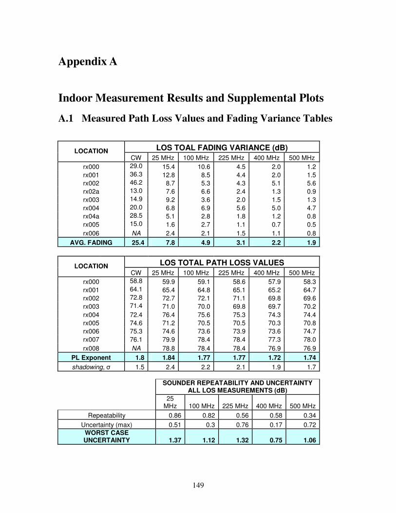
A.1 Measured Path Loss Values and Fading Variance Tables...................................................... 149
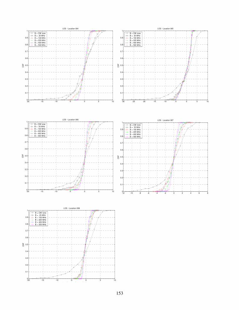
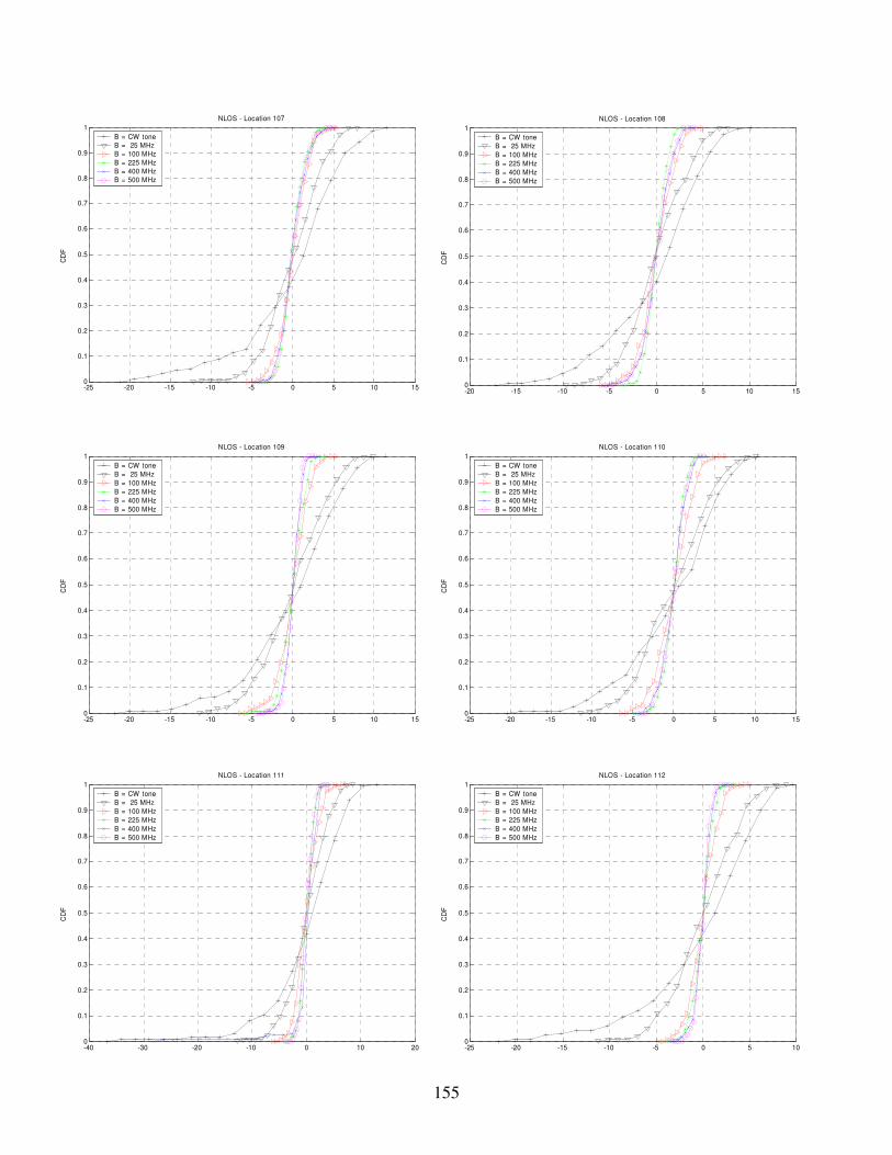
A.2 Small Scale Fading Results........................................................................................................ 152 A.2.1 Normalized Received Power CDF Plots for LOS Locations................................................... 152 A.2.2 Normalized Received Power CDF Plots for NLOS Locations................................................ 154 A.2.3 Nakagami-m Fading Parameters for Received Power PDFs ................................................... 157
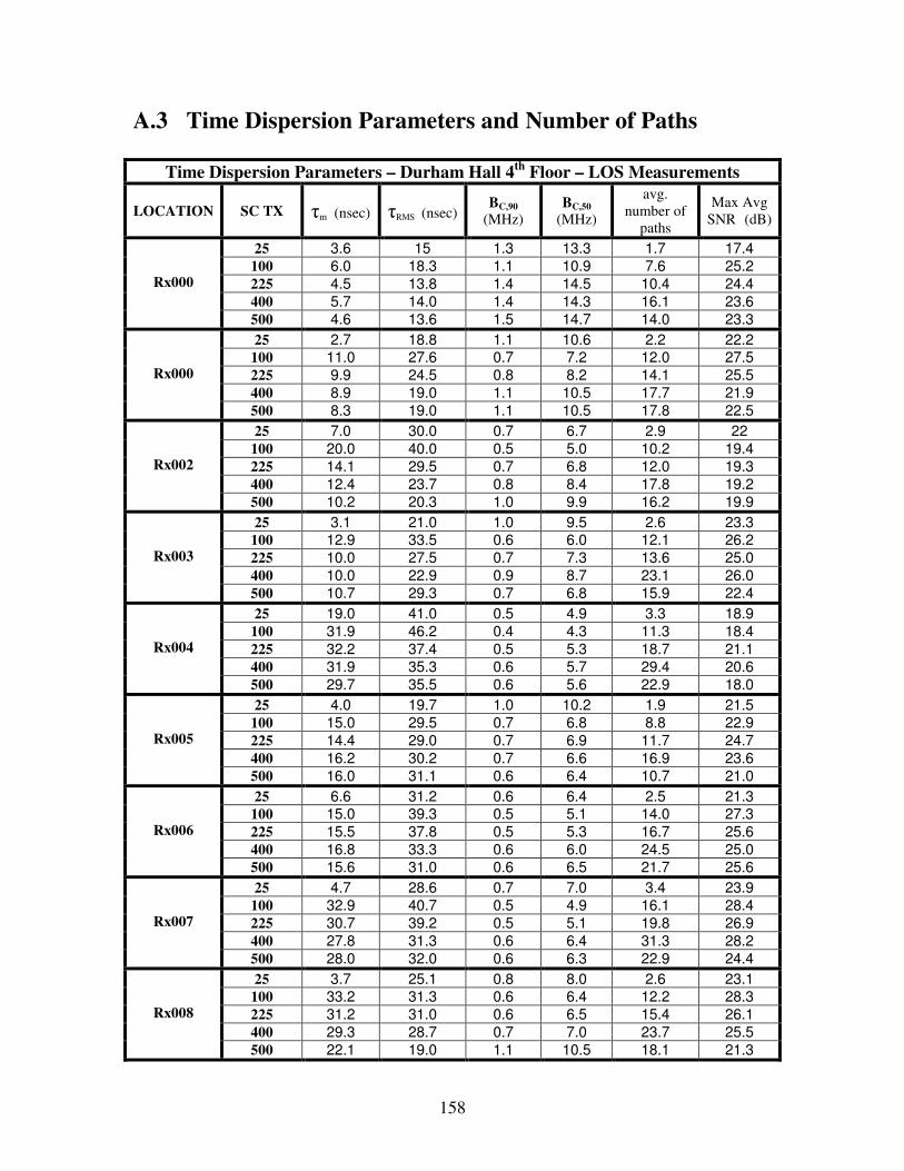
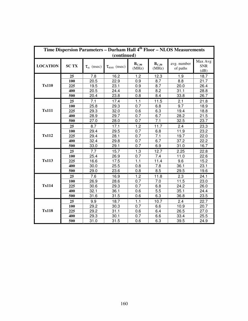
A.3 Time Dispersion Parameters and Number of Paths................................................................ 158
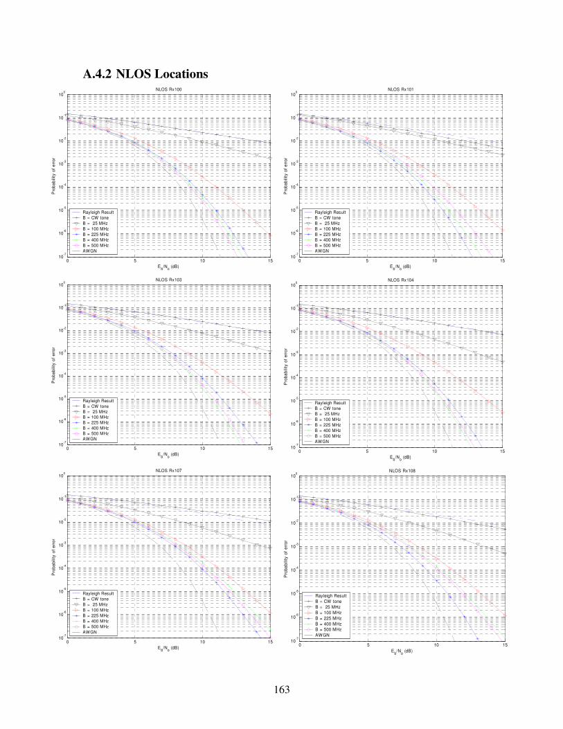
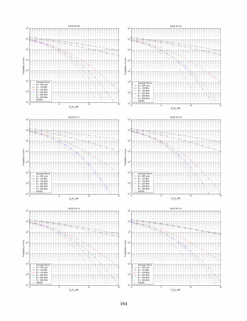
A.4 Probability of Error vs. Eb/No for BPSK Modulation ............................................................. 161 A.4.1 LOS Locations......................................................................................................................... 161 A.4.2 NLOS Locations...................................................................................................................... 162 A.4.2 NLOS Locations...................................................................................................................... 163
APPENDIX B
DERIVATION OF INSTANTANEOUS WIDEBAND RECEIVED POWER IN A 2 PATH FADING CHANNEL...............................................................................166
APPENDIX C
ANTENNA POSITIONING SYSTEM USER GUIDE AND REFERENCE .........170
C.6 Positioning System Suggested Upgrades .................................................................................. 183
C.7 APAC System Requirements and Additional Support ........................................................... 184 C.7.1 System Requirements .............................................................................................................. 184 C.7.2 Converting User Parameters to 2-D Grid Definition ............................................................... 185 C.7.3 System Specific Parameters .................................................................................................... 186 C.7.4 A Note on Modifying APAC for Fast Acquisition .................................................................. 187 C.7.5 APAC Suggested Upgrades..................................................................................................... 187
LIST OF TABLES Table 2.1 – Mitigation bandwidth per chip rate for various modulation schemes. ...................................... 34 Table 3.1 – Sliding correlator system parameters and their dependence on PN sequence properties, from [1]
and [5]. Essentially all the capabilities and limitations of the system are dictated by the PN length and transmitter and receiver clock frequencies. .................................................................................. 50
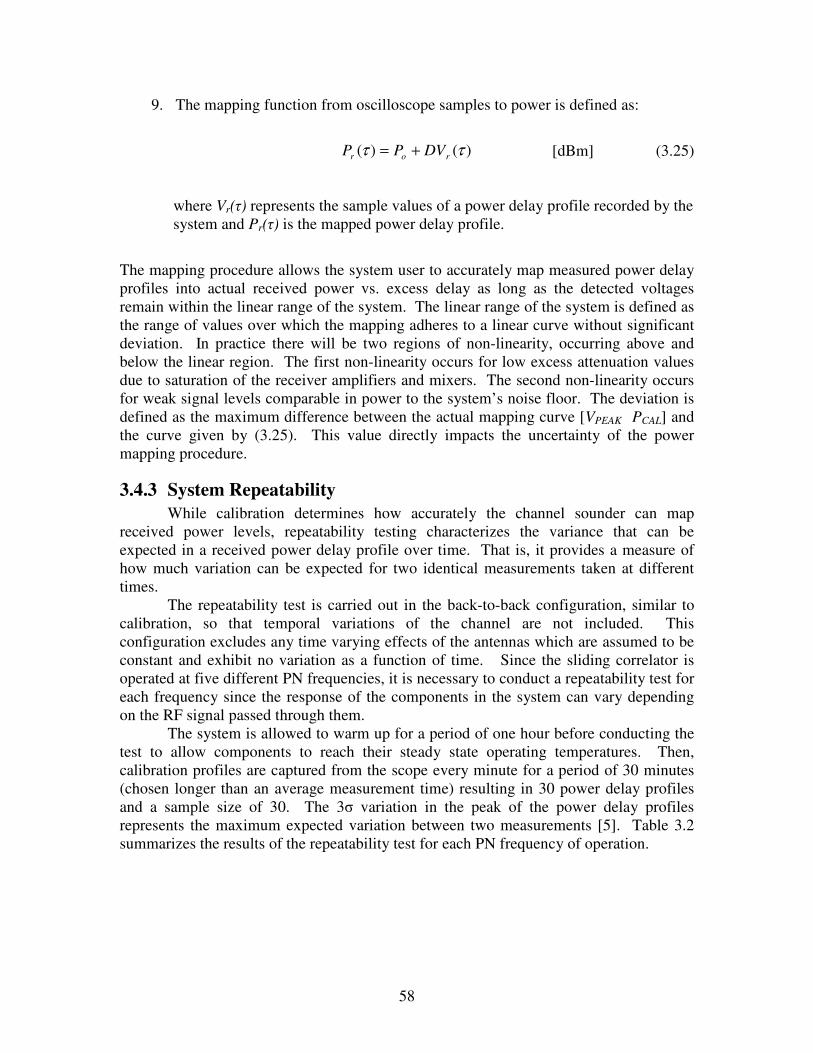
Table 3.2 – Repeatability for the MPRG sliding correlator channel sounder at 2.5 GHz and PN frequencies
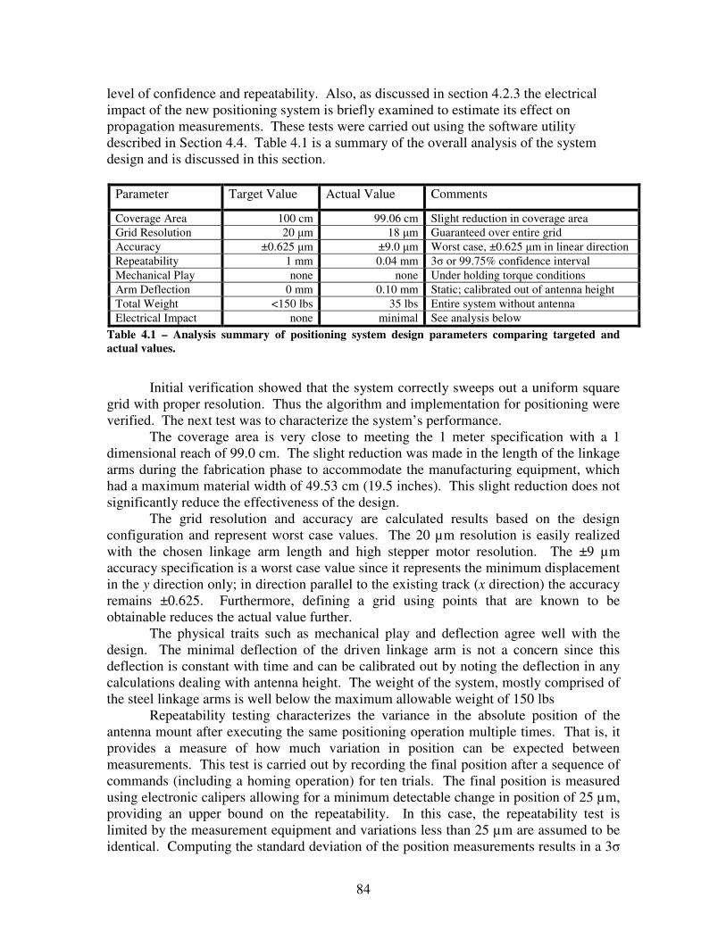
of operation ......................................................................................................................................... 59 Table 4.1 – Analysis summary of positioning system design parameters comparing targeted and actual
values. ................................................................................................................................................. 84 Table 5.1 – Sliding correlator configurations and performance metrics ...................................................... 89 Table 5.2 – 1 meter free space references for the wideband channel sounder configurations ..................... 89 Table 5.3 – TR separation distances for LOS locations, distance measured to the center of the receive grid.
............................................................................................................................................................ 92 Table 5.4 - TR separation distances for LOS locations, distance measured to the center of the receive grid.
For receiver locations refer to Figures 5.6 – 5.10. .............................................................................. 93 Table 5.5 – Peak path loss exponent and shadowing term for LOS configurations with TR separation
between 1 and 16.8 m exhibiting free space propagation ................................................................... 98 Table 5.6 – The normalized received power fading variance for six spreading bandwidths in LOS and
NLOS channels. UWB results taken from [33]............................................................................... 103 Table 5.7 – The impact of measurement spacing on calculated fading variance for CW and 500 MHz
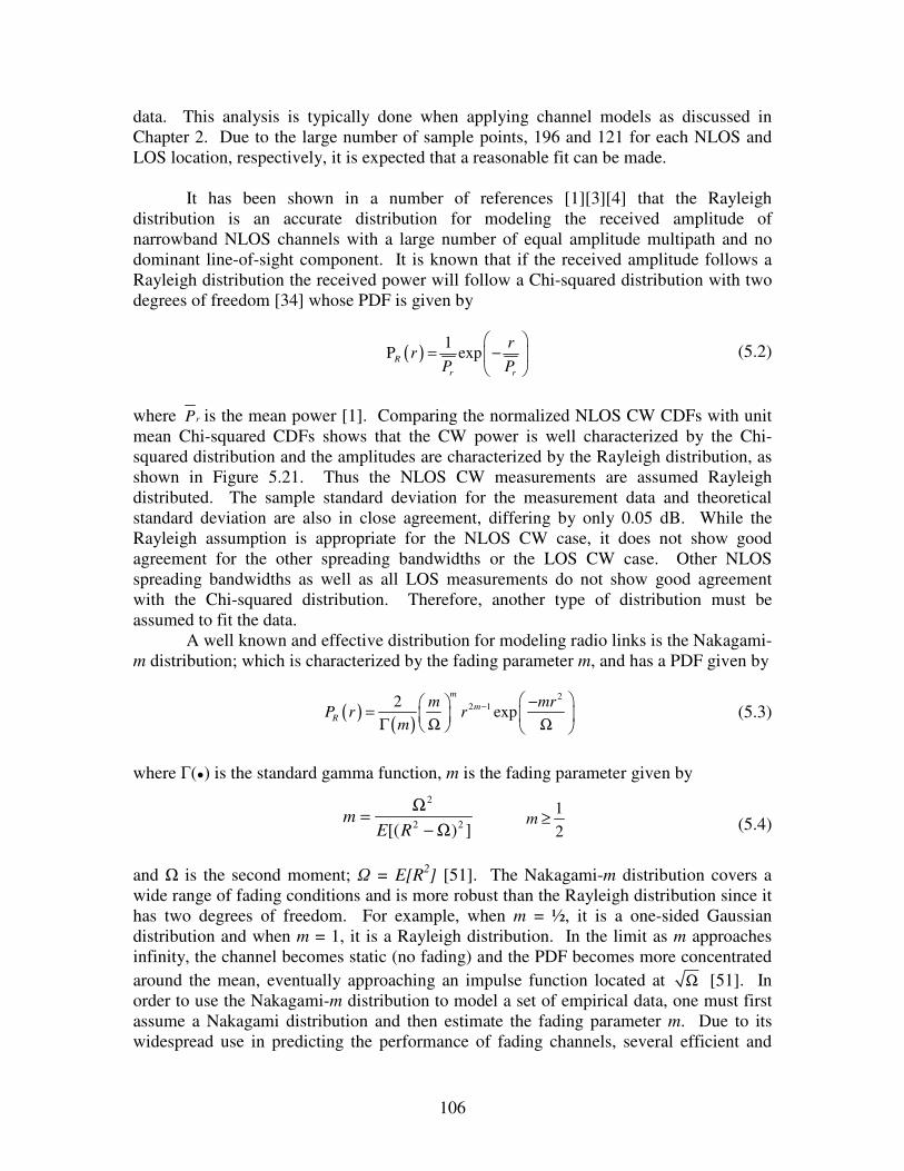
spreading bandwidths in a NLOS channel. ....................................................................................... 105 Table 5.8 – Nakagami-m fading parameter estimation using estimator from [52] for LOS and NLOS
channels ............................................................................................................................................ 108 Table 5.9 – Average time dispersion parameters and average number of components for the LOS and
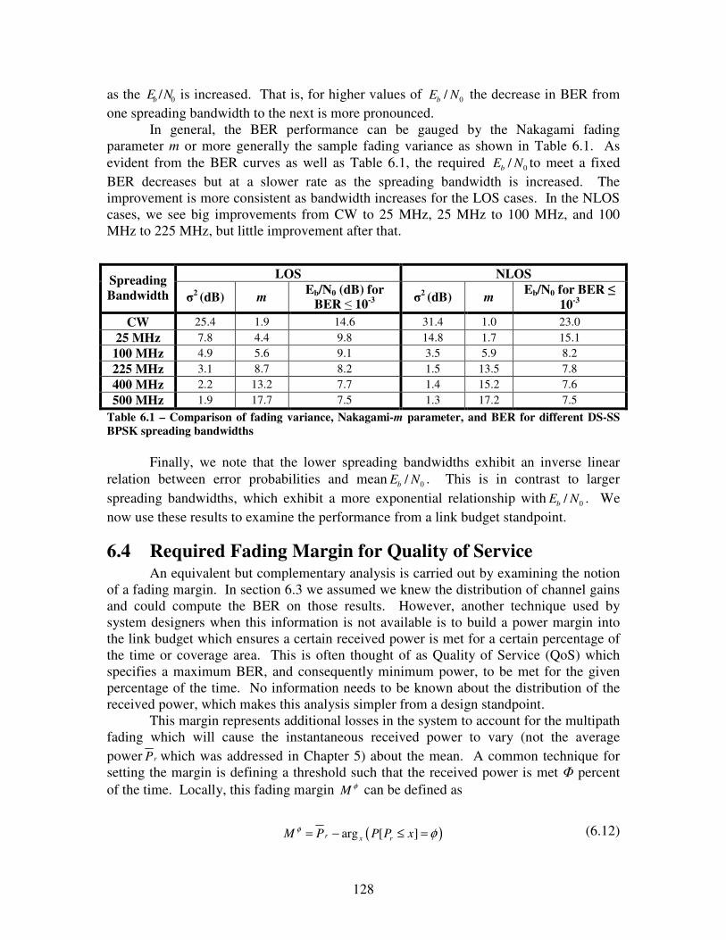
NLOS locations. UWB results are taken from [33]. ........................................................................ 110 Table 6.1 – Comparison of fading variance, Nakagami-m parameter, and BER for different DS-SS BPSK
spreading bandwidths........................................................................................................................ 128 Table 6.2 – Fading Margin for 90, 95, and 99 percent probability the mean power is achieved at the
receiver input for measured LOS and NLOS .................................................................................... 129 Table 6.3 – Advantage in using two antenna selection diversity over a single antenna at the receiver for
BPSK ................................................................................................................................................ 131 Table 6.4 – BPSK performance of an ideal Rake receiver which has unlimited countable correlators to
capture 95% of the total available power .......................................................................................... 134
x
Table 6.5 – Comparison of observed and predicted optimal pilot-to-data channel ratio () for a BPSK BER of 10-2 in measured fading channels.................................................................................................. 136
Table 6.6 – Impact of channel estimation on BPSK BER performance for five spreading bandwidths and
four different PDR ratios................................................................................................................... 138 Table 6.7 – Nakagami-m fading parameter for all speading bandwidths and five strongest paths. These
values reflect the entire NLOS data set............................................................................................. 140 Table 6.8 – Comparison of optimal spreading bandwidth which minimize the required Eb/N0 to meet a 10-3
BER using BPSK modulation; assuming perfect channel estimation. .............................................. 142 Table 6.9 – Comparison of optimal spreading bandwidth which minimize the required Eb/N0 to meet a 10-3
BER using BPSK modulation; with channel estimation and = 0.25. ............................................. 142 Table C.1 – Suggested maximum values for positioning system in native configuration. See [15] for a
complete definition of commands..................................................................................................... 171 Table C.2 – Directory structure for proper operation of APAC ................................................................ 185
xi
LIST OF FIGURES Figure 2.1 – Huygens’ Principle applied to the propagation of plane waves in a lossless medium............. 12 Figure 2.2 – Huygens’ Principle applied to diffraction at the edge of a sharp obstacle............................... 12 Figure 2.3 – Fresnel zone geometry. Concentric circles define the boundaries of successive Fresnel zones.
............................................................................................................................................................ 13 Figure 2.4 – Examples of time varying (left) and time invariant (right) discrete time channel impulse
responses. ............................................................................................................................................ 21 Figure 3.1 – Block diagram of a PN sequence generator............................................................................. 45 Figure 3.2 – The normalized auto correlation function of a maximal length PN sequence with the auto
correlation waveform superimposed over the discrete values. The dimensions have been exaggerated for emphasis. ....................................................................................................................................... 45
Figure 3.3 – Basic functional blocks of a spread spectrum sliding correlator measurement system
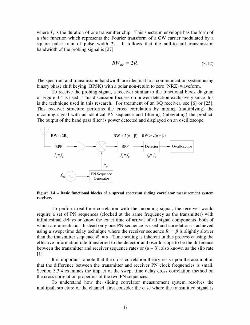
transmitter. .......................................................................................................................................... 46 Figure 3.4 – Basic functional blocks of a spread spectrum sliding correlator measurement system receiver.
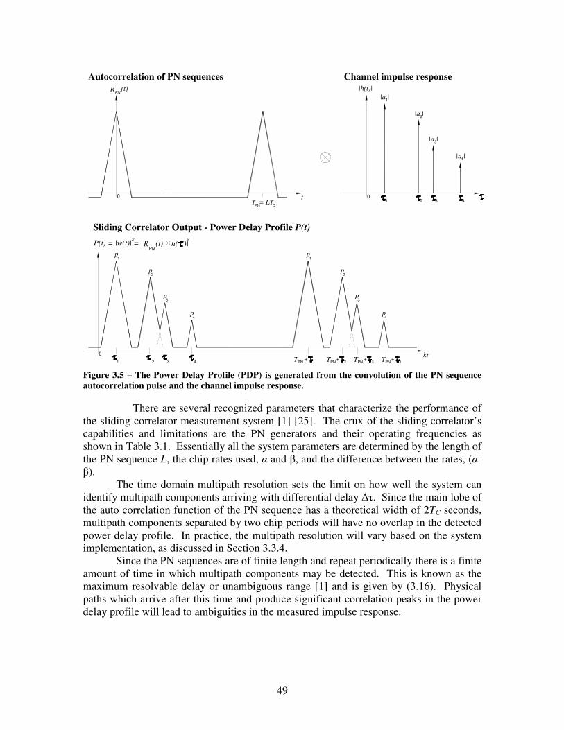
............................................................................................................................................................ 47 Figure 3.5 – The Power Delay Profile (PDP) is generated from the convolution of the PN sequence
autocorrelation pulse and the channel impulse response..................................................................... 49 Figure 3.6 – Sliding correlator correlation peak widening and reduction (a) and dynamic range reduction
(b) using the simulation algorithm from [31]...................................................................................... 52 Figure 3.7 – Sliding correlator transmitter as implemented at Virginia Tech for this research. .................. 54 Figure 3.8 – Sliding correlator receiver as implemented at Virginia Tech for this research. ...................... 55 Figure 3.9 – Functionality of the spectrum analyzer in the sliding correlator receiver. The spectrum
analyzer completes the correlation and produces an output voltage proportional to the received power. ................................................................................................................................................. 56
Figure 4.1 – Existing Parker Automation linear table with rotary table mounted on carriage. The entire
assembly is mounted on a utility table. ............................................................................................... 65 Figure 4.2 –PDX indexers (left) and RS-232 interface (right) for controlling the linear and rotary tables. 65 Figure 4.3 – Illustration of a novel positioning technique using a rotating boom mounted on a linear track,
with uniform grid spacing s in both the x and y directions. ................................................................ 67 Figure 4.4 – Maintaining constant relative position using a 4-bar parallel linkage system in place of a
boom. The base linkage is held fixed and black dots denote points free to rotate. ............................ 69 Figure 4.5 – Moment curve for Parker Automation rotary positioning table. The curve indicates the
maximum end load for linkage arm length, from [17]. ....................................................................... 70 Figure 4.6 – Linkage base component 1. This component facilitates connection of the driven arm to the
rotary table. Scale and dimensions are given in Appendix C.............................................................. 71
xii
Figure 4.7 – Linkage base component 2. This component facilitates connection of the idler arm to the fixed portion of the rotary table while maintaining sufficient clearance of the rotating table. Scale and dimensions are given in Appendix C. .......................................................................................... 71
Figure 4.8 – Antenna mount linkage with mounting holes facilitating connection of various antennas. Scale
and dimensions are given in Appendix C. .......................................................................................... 72 Figure 4.9 – Top view scale rendering of the assembled 4-bar parallel linkage positioning system mounted
on the existing Parker Automation rotary table. Scale and dimensions are given in Appendix C. .... 72 Figure 4.10 – Finalized 4-bar parallel linkage antenna positioning system installed on existing Parker
Automation equipment, final configuration shown at right (with PC running APAC control application). ........................................................................................................................................ 74
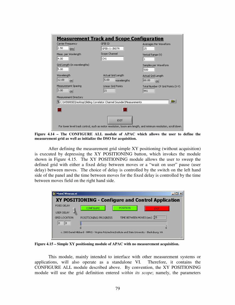
Figure 4.11 – Antenna positioning system grid layout and orientation to the x and y axis. ........................ 75 Figure 4.12 – Algorithm for moving the positioning system over the grid using [i], d[i], and sa[i]......... 76 Figure 4.13 - Antenna Positioning and Acquisition Control Application (APAC) front panel ................... 78 Figure 4.14 – The CONFIGURE ALL module of APAC which allows the user to define the measurement
grid as well as initialize the DSO for acquisition................................................................................ 79 Figure 4.15 – Simple XY positioning module of APAC with no measurement acquisition........................ 79 Figure 4.16 – Track log file information panel of the CREATE LOG AND TRACK LOCATION module,
adapted from an undergraduate research project described in [5]....................................................... 80 Figure 4.17 – Calibration utility of APAC used for calibrating the sliding correlator measurement system.
............................................................................................................................................................ 82 Figure 4.18 – Repeatability utility of APAC used for estimating the repeatability of the sliding correlator
channel sounder. ................................................................................................................................. 82 Figure 4.19 – PDX terminal module of APAC used to return positioning system to home position if left in
an unknown state................................................................................................................................. 83 Figure 5.1 – CW channel sounder configured for power measurements at 2.5 GHz................................... 88 Figure 5.2 – Measurement grid and orientation with positioning equipment for NLOS (left) and LOS
(right) measurements. The large black dot denotes the position of the (0,0) point. ........................... 90 Figure 5.3 – Floor plan of the fourth floor of Durham Hall with NLOS and LOS locations outlined......... 91 Figure 5.4 – LOS transmitter and receiver locations for receiver locations Rx000 – Rx004. The black dot
on the receiver grid denotes the location of grid point (0,0). .............................................................. 92 Figure 5.5 - LOS transmitter and receiver locations for receiver locations Rx005– Rx008. The black dot
on the receiver grid denotes the location of grid point (0,0). .............................................................. 93 Figure 5.6 - NLOS transmitter and receiver locations for receiver location 1. The black dot on the receiver
grid denotes the location of grid point (0, 0)....................................................................................... 94
xiii
Figure 5.7 - NLOS transmitter and receiver locations for receiver location 2. The black dot on the receiver grid denotes the location of grid point (0, 0)....................................................................................... 94
Figure 5.8 - NLOS transmitter and receiver locations for receiver location 3. The black dot on the receiver
grid denotes the location of grid point (0, 0)....................................................................................... 94 Figure 5.9 - NLOS transmitter and receiver locations for receiver location 4. The black dot on the receiver
grid denotes the location of grid point (0, 0)....................................................................................... 95 Figure 5.10 - NLOS transmitter and receiver locations for receiver location 5. The black dot on the
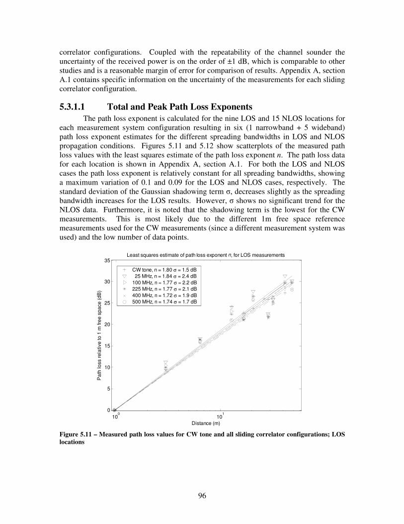
receiver grid denotes the location of grid point (0,0). ......................................................................... 95 Figure 5.11 – Measured path loss values for CW tone and all sliding correlator configurations; LOS
locations .............................................................................................................................................. 96 Figure 5.12 - Measured path loss values for CW tone and all sliding correlator configurations; NLOS
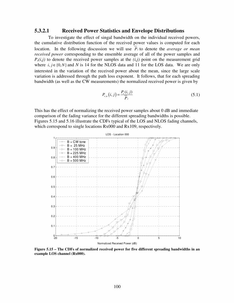
locations .............................................................................................................................................. 97 Figure 5.13 - Measured peak path loss values for all sliding correlator configurations; LOS locations ..... 98 Figure 5.14 - Measured peak path loss values for all sliding correlator configurations; NLOS locations... 99 Figure 5.15 – The CDFs of normalized received power for five different spreading bandwidths in an
example LOS channel (Rx000)......................................................................................................... 100 Figure 5.16 – The CDFs of normalized received power for five different spreading bandwidths in an
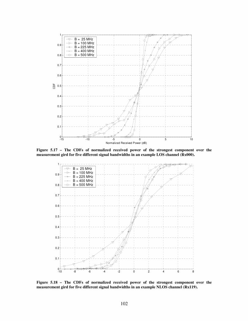
example NLOS channel (Rx109). ..................................................................................................... 101 Figure 5.17 – The CDFs of normalized received power of the strongest component over the measurement
gird for five different signal bandwidths in an example LOS channel (Rx000). .............................. 102 Figure 5.18 – The CDFs of normalized received power of the strongest component over the measurement
gird for five different signal bandwidths in an example NLOS channel (Rx109)............................. 102 Figure 5.19 – Comparison of received power for CW and 500 MHz spreading bandwidths in a NLOS
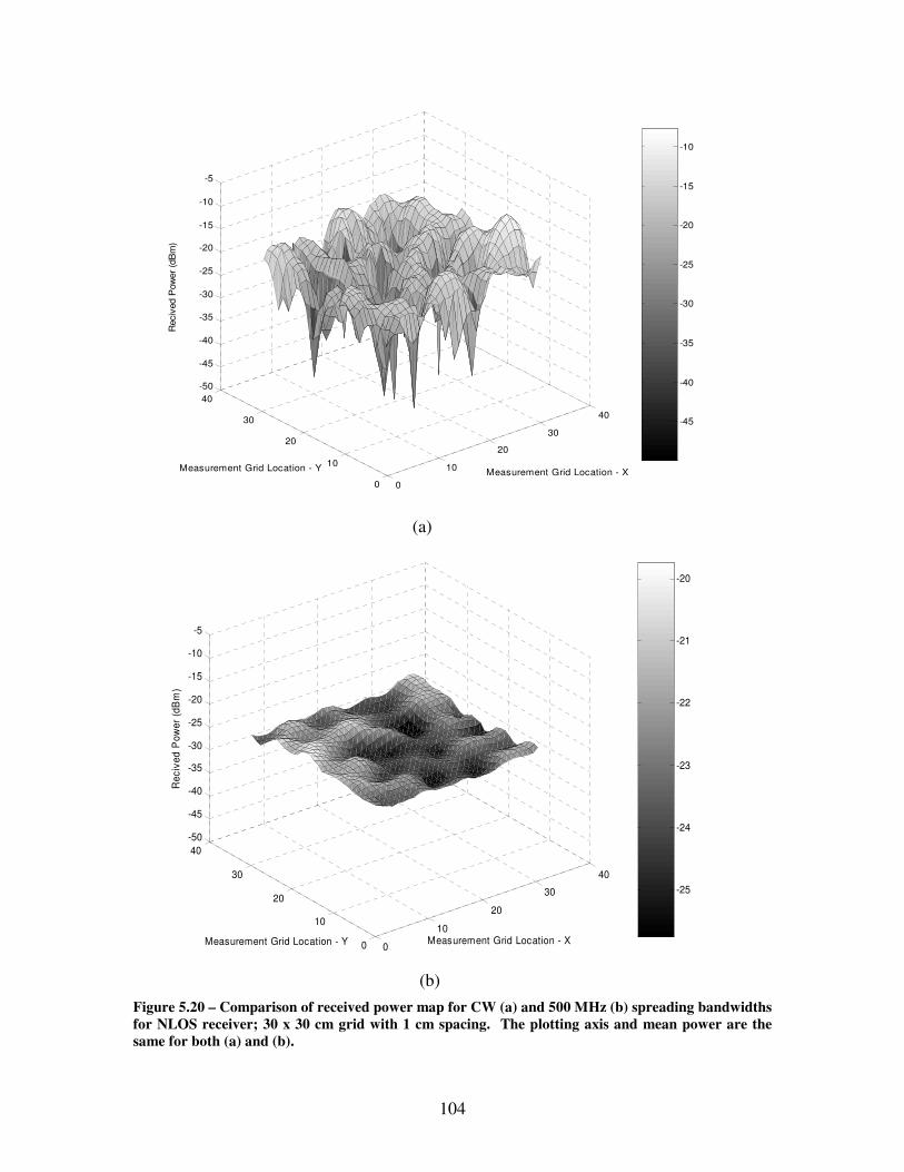
channel (the mean power is the same for both signals).......................................................................103 Figure 5.20 – Comparison of received power map for CW (a) and 500 MHz (b) spreading bandwidths for
NLOS receiver; 30 x 30 cm grid with 1 cm spacing. The plotting axis and mean power are the same for both (a) and (b)............................................................................................................................ 104
Figure 5.21 – Comparison of CW measurements with (a) Rayleigh PDF and (b) Chi-squared CDF for a
typical NLOS channel. Plots (c) and (d) compare measured data with fitted Nakagami-m distribution for a typical NLOS channel with m = 6.4 and m = 29, respectively. ................................................ 107
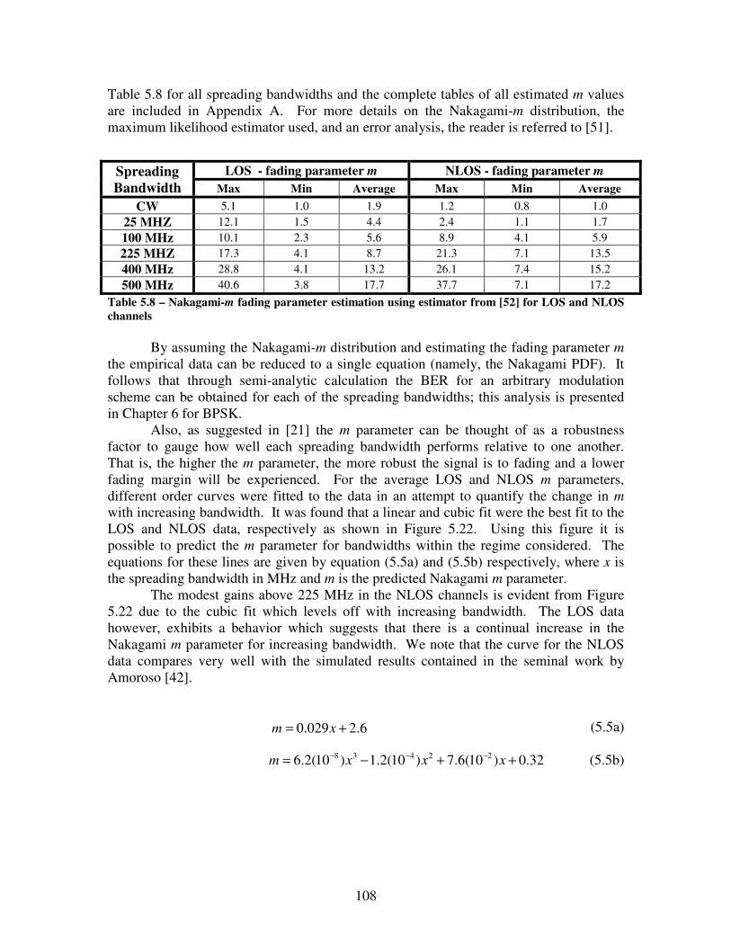
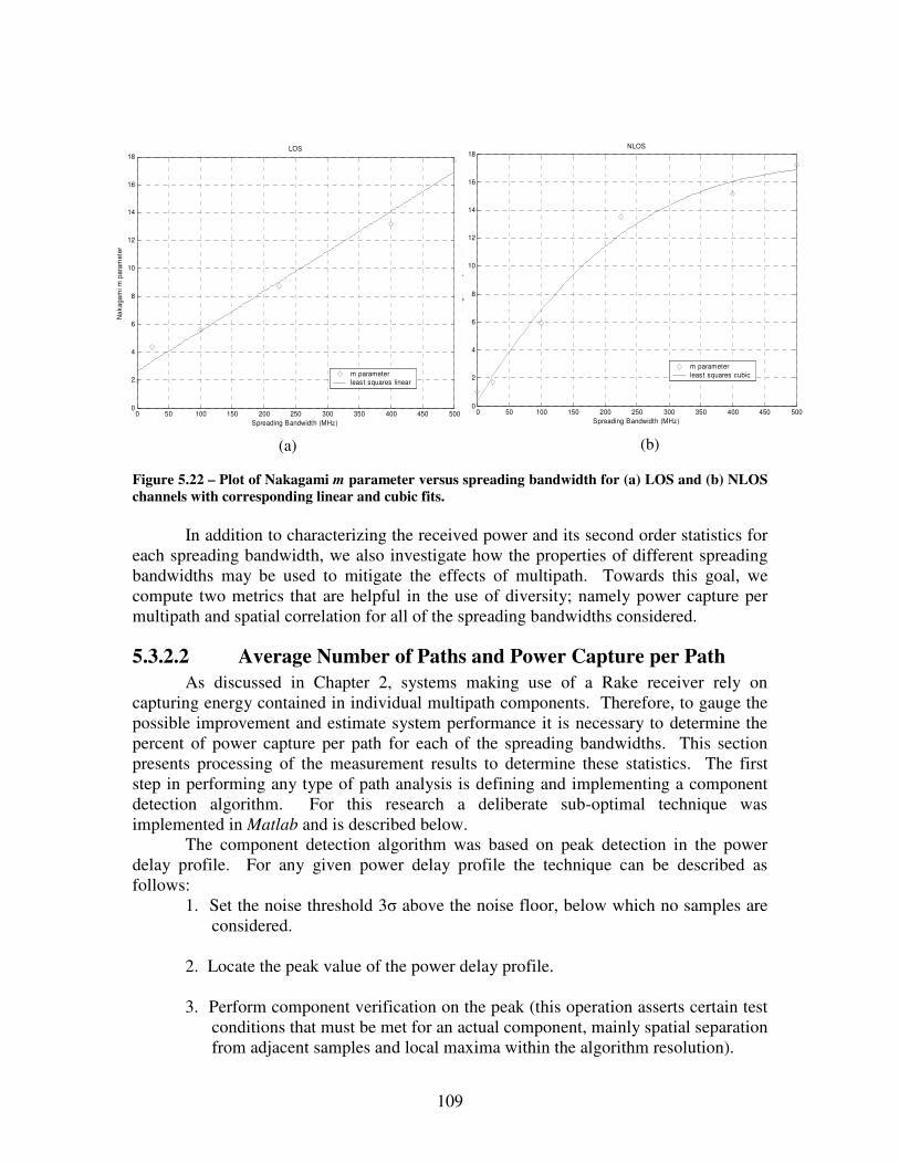
Figure 5.22 – Plot of Nakagami m parameter versus spreading bandwidth for (a) LOS and (b) NLOS
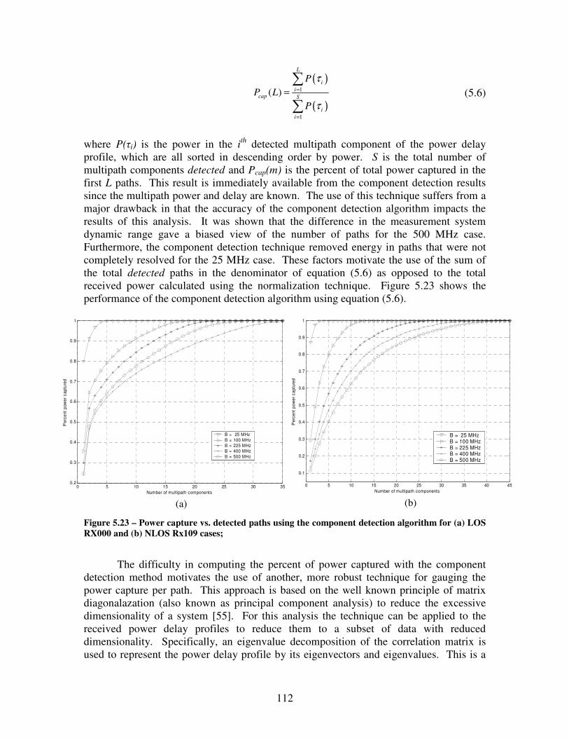
channels with corresponding linear and cubic fits. ........................................................................... 109 Figure 5.23 – Power capture vs. detected paths using the component detection algorithm for typical LOS
(a) and NLOS (b) cases..................................................................................................................... 112 Figure 5.24 – Percent energy capture versus the number of eigenvalues for a typical LOS channels....... 114
xiv
Figure 5.25 – Percent energy capture versus the number of eigenvalues for a typical NLOS channels
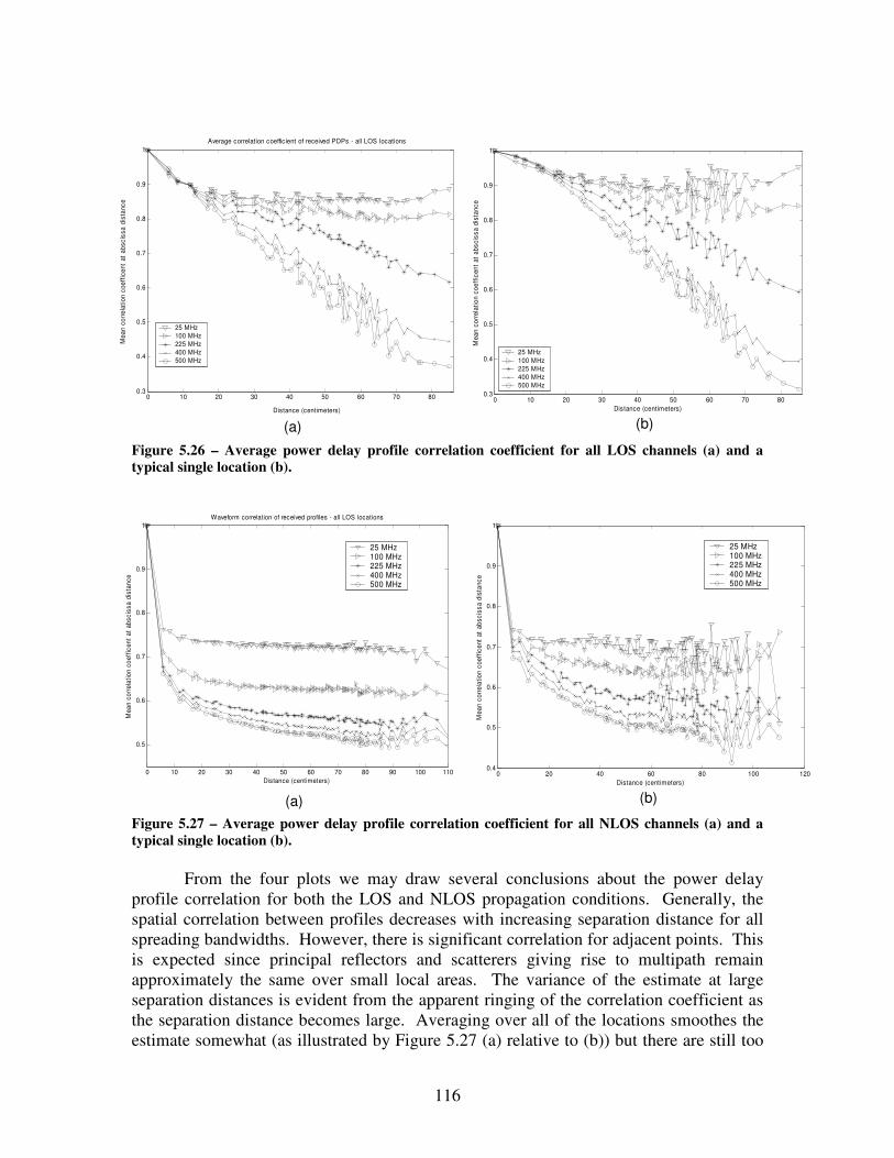
measured. .......................................................................................................................................... 114 Figure 5.26 – Average power delay profile correlation coefficient for all LOS channels (a) and a typical
single location (b). ............................................................................................................................ 116 Figure 5.27 – Average power delay profile correlation coefficient for all NLOS channels (a) and a typical
single location (b). ............................................................................................................................ 116 Figure 5.28 – Co-located Power Delay Profiles for 25 MHz (a) and 500 MHz (b) spreading bandwidths,
grid spacing of 6 cm.......................................................................................................................... 117 Figure 5.29 – Average received power correlation coefficient for all LOS channels (a) and NLOS channels
(b). This curve represents the correlation between the total received power values over the measurement grid.............................................................................................................................. 118
Figure 5.30 – Local average PDP for LOS receiver at location 007 showing four significant multipath
components. ...................................................................................................................................... 119 Figure 5.31 –PDP correlation coefficient over the measurement grid for 25 MHz (a) and 500 MHz (b) for
the LOS Rx005 (large open area in the corridor). The reference point at for which all coefficients are calculated is denoted by X and color intensity corresponds to correlation coefficient magnitude. (c) and (d) correspond to LOS Rx007 for 25 MHz and 500 MHz, respectively..................................... 120
Figure 6.1 – Bit Error Rate performance of un-coded DS-SS BPSK for different spreading bandwidths in a
LOS Nakagami fading channel ......................................................................................................... 126 Figure 6.2 – Bit Error Rate performance of un-coded DS-SS BPSK for different spreading bandwidths in a
NLOS Nakagami fading channel ...................................................................................................... 126 Figure 6.3 – Comparison between semi-analytic and stochastic average techniques for computing the BER
in measured channels for CW (a) and 500 MHz (b) spreading bandwidths...................................... 127 Figure 6.4 – Determining the fading margin M from the CDF of the normalized received power; LOS (a)
and NLOS (b) data. ........................................................................................................................... 129 Figure 6.5 – Performance gain for CW and 500 MHz spreading bandwidth when two element antenna
selection diversity is employed at the receiver (a) CDF and (b) BER (BPSK). The dashed line represents the case where selection diversity is used. ....................................................................... 132
Figure 6.6 – Number of multipath components required for 95 percent power capture at NLOS location
Rx112................................................................................................................................................ 133 Figure 6.7 – Impact of channel estimation on BPSK BER performance for 25 MHz and 500 MHz
spreading bandwidths with two different pilot-to-data channel ratios ()......................................... 137 Figure 6.8 – BPSK BER performance for a single finger SRake receiver for measured spreading
bandwidths ........................................................................................................................................ 139 Figure 6.9 - BPSK BER performance for a five finger SRake receiver for measured spreading bandwidths
Figure 6.10 – BPSK BER performance for a 25 finger SRake receiver for measured spreading bandwidths.......................................................................................................................................................... 141
Figure 6.11 – BPSK BER performance for a single finger SRake receiver for measured spreading
bandwidths including the degradation due to channel estimation..................................................... 143 Figure 6.12 – BPSK BER performance for a five finger SRake receiver for measured spreading
bandwidths including the degradation due to channel estimation..................................................... 143 Figure C.1 – Driven arm support and idler arm offset components made as modifications to the original
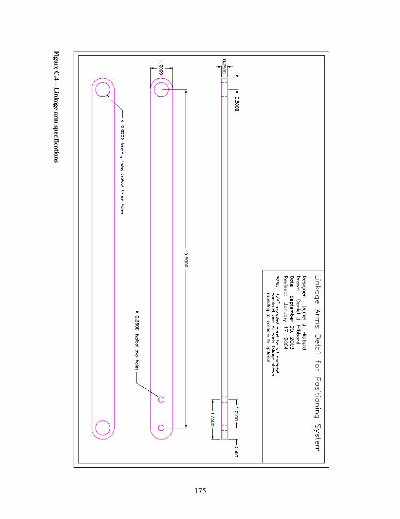
design. ............................................................................................................................................... 171 Figure C.2 – Driven arm linkage base mount specifications........................................................................................173 Figure C.3 – Idler arm linkage base mount specifications.............................................................................................174 Figure C.4 – Linkage arm specifications..............................................................................................................................175 Figure C.5 – Antenna mount linkage specifications........................................................................................................176 Figure C.6 – Top, front, right side AutoCAD rendering of 4-bar parallel linkage system................................177
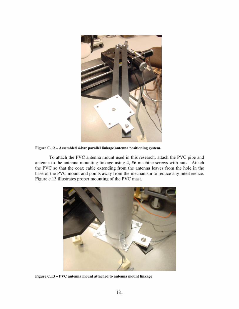
Figure C.7 – Linear and rotary table in home position prior to system installation .................................. 178 Figure C.8 – Rotary table with idler arm base linkage mounted to rotary table base................................ 178 Figure C.9 - Rotary table with driven arm base linkage mounted ............................................................. 179 Figure C.10 – Idler arm offset mounted to idler arm linkage base ............................................................ 179 Figure C.11 – Attaching the linkage arms to the rotary table via the base linkage mounts....................... 180 Figure C.12 – Assembled 4-bar parallel linkage antenna positioning system. .......................................... 181 Figure C.13 – PVC antenna mount attached to antenna mount linkage .................................................... 181 Figure C.14 – Grid spacing convention used to derive measurement spacing from measurements per
wavelength. ....................................................................................................................................... 186 Figure C.15 – Configuration options that can only be accessed through opening the sub_configure_track
VI separately and scrolling down. In the native configuration, these parameters will never change........................................................................................................................................................... 187
xvi
LIST OF ABBREVIATIONS
AOA Angle of Arrival APAC Antenna Positioning and Acquisition Control AWGN Additive White Gaussian Noise BER Bit Error Rate BPSK Binary Phase Shift Keying CDF Cumulative Distribution Function CDMA Code Division Multiple Access CIR Channel Impulse Response CW Continuous Wave DOA Direction of Arrival DS-SS Direct Sequence Spread Spectrum EGC Equal Gain Combining FDMA Frequency Division Multiple Access LOS Line-Of-Sight MRC Maximal Ratio Combining NLOS Non-Line-Of-Sight OFDM Orthogonal Frequency Division Multiplexing PDF Probability Density Function PDP Power Delay Profile PDR Pilot-to-Data channel Ratio PL Path Loss PN Pseudorandom Noise PSD Power Spectral Density QoS Quality of Service SC Sliding Correlator SNR Signal to Noise Ratio SS Spread Spectrum TDMA Time Division Multiple Access UWB Ultra-Wideband VI Virtual Instrument VSWR Voltage Standing Wave Ratio
1
Chapter 1
Introduction and Thesis Overview
1.1 Motivation In general, a wireless communication system is a means for transmitting unknown
data without errors from one location to another without the use of guiding structures, and such systems have been around for over a hundred years. Since the early work of Guglielmo Marconi [60] in ship-to-shore communications, the advancement of wireless communications has come an extremely long way. After the “wired” barrier was broken at the turn of the nineteenth century, the mobile barrier was broken with the advent of transistors in the 1940s and 50s which allowed for compact receiver designs. Since then, continual advancements have been made in the area of wireless portable communication systems, specifically in the area of reducing the cost of such devices, but also in the underlying technology. A challenge probably never envisioned by Marconi, but the bane of many of today’s wireless researches is coping with the increasing number of users and systems in the dwindling radio spectrum, while addressing the desire for faster, more robust systems. To this end, the research community has addressed ways in which these new challenges can be met and this thesis represents a contribution towards that goal.
Over the past several years, there has been a significant amount of interest and research in the area of wideband and ultra-wideband (UWB) signaling for use in indoor wireless systems1. This interest is in part motivated by the fact that the use of large bandwidth signals makes systems less sensitive to the degrading effects of multipath propagation, which often typifies the indoor environment. By reducing the sensitivity to multipath, more robust and higher capacity systems can be realized. Additionally, these wideband and UWB techniques are well suited for multiple access and deployment over existing narrowband communication systems which makes them a viable candidate for future systems in the dwindling radio spectrum. Recent rulings by the FCC allowing the use of certain types of unlicensed UWB further support the future potential of such technologies.
The notion on which this entire work is based (larger bandwidths mean less fading) is well known in the area of communication research. However, there exist very few studies which definitively characterize and study this effect; and even fewer which are based on actual measurement data. This work presents a complete analysis of this well known phenomenon which to the author’s knowledge has not been done with this type of scope before.
1 Wideband and Ultra-Wideband signals are defined shortly, but for this discussion they can be thought of as signals having bandwidths much larger than current digital systems which are on the order of kHz.
2
1.2 Background and Perspective The background required for this thesis is minimal, and it is expected that
someone with a general understanding of communication principles as well as basic mathematics, probability theory and stochastic processes can grasp and benefit from its content. In instances where specialized concepts are presented, they are either explained or references given where the reader can find excellent treatment of the material. However, for the benefit of the reader it is useful to consider how the work in this thesis fits into the big picture of wireless communications.
The main reason for interest in this thesis topic lies in its application to direct sequence spread spectrum (DS-SS) communication systems, specifically DS-CDMA. Code Division Multiple Access or CDMA is a multiple access technique that allows multiple users to share the radio spectrum at the same time, over the same frequency. This is in comparison to frequency division multiple access (FDMA), in which the frequency spectrum is divided into sections for use by only one user at a time or time division multiple access (TDMA), in which the same portion of the radio spectrum is shared by multiple users at different times. Traditional broadcast radio and television are examples of systems using FDMA while push-to-talk short range walkie-talkie type devices usually use TDMA (only one person is allowed to talk at a time). CDMA is one of the major current standards deployed for commercial wireless telephone (IS-95) and has future potential for wideband and UWB systems based on its many strengths for coexisting systems. In a CDMA system, narrowband information signals are “spread” by multiplying them with a known pseudorandom noise (PN) sequence which makes them similar to white Gaussian noise when transmitted. However, since the PN sequence is known, the signal can be “despread” at the receiver by multiplying the incoming signal with the same PN sequence. The properties of the codes are such that different codes have low correlation to one another and multiple codes can be sent and demodulated over the same time/frequency channel, which is only limited by the effective increase in noise. CDMA inherently provides a mechanism for diversity or the combining of multipath versions of the originally transmitted signal separated in time to increase performance. This mechanism is inherent due to the use of PN sequences, and will be discussed in Chapter 2; however we note here that there is a specific type of receiver architecture known as the Rake receiver which can be used to exploit this benefit.
It is the performance of these systems we are particularly interested in for this research work. Namely, we will assume that we are dealing with a CDMA system in which the required data rate has been met for a small spreading bandwidth and the next decision in the system design is how wide one spreads the signal for transmission over the channel. Or, we assume that a high data rate system with an inherently large signal bandwidth is being used, and the additional spreading is minimal or non-existent; this would be the case of a UWB system. The choice of the spreading bandwidth will impact the system in a number of ways, including the optimal receiver design and expected performance in different environments. Therefore, the ultimate goal from a communication engineering standpoint is to provide meaningful metrics to make this decision as well as quantify the performance for different spreading bandwidths. This thesis aims to do that by investigating the performance of a number of spreading bandwidths in an indoor propagation environment, ranging from narrowband (several hundred kHz) to ultra-wideband (bandwidths in excess of 1 GHz).
3
When providing these metrics one must never forget that they are merely statistical quantities which attempt to explain the complex behavior of the propagation channel. In general, the mechanisms that affect propagating waves are well understood but when applied to the highly random indoor environment they are hard to combine to yield meaningful results. This leads to the notion of a gap between the theory of wave propagation and channel characterizations with immediate application to system design. Traditionally, this gap has been bridged by simulation, deterministic models, simplifications, or perhaps the most common, statistical characterization based on measurements. The latter is the approach mostly considered in this thesis, but the author notes that bridging this gap in more deterministic ways is perhaps more beneficial towards a unified understanding of the propagation medium. While it is beyond the scope of this thesis to “bridge the gap”, this work presents the basic principles of propagation in Chapter 2 in an effort to shed more light on what is actually taking place in the indoor environment. A note on site specific phenomenon is also presented in Chapter 5. Knowing these mechanisms and attempting to apply them to observed results is the first step in truly gaining a physical understanding of the wireless channel.
1.3 Thesis Overview The general purpose of this thesis work is to provide an analysis of the impact
signal bandwidth has on indoor wireless systems. As with any focused research effort, the ultimate goal is to provide meaningful results from which the research community in general can benefit from. To that end, this thesis is laid out in a manner to clearly demonstrate the work completed as well as provide meaningful results for future use.
Chapter 2 is intended to serve as an introduction and review to some of the core principles in the physical layer of wireless communication systems. It begins with a review of the basic propagation mechanisms affecting waves in a practical environment, followed by the development of the basic link equation for a communication system. This chapter also covers large scale and small scale channel characterization, and the generally accepted parameters used to do such. Fading and multipath mitigation techniques are briefly covered. Finally, a literature review of the past and current works in the area, impacting spreading bandwidth on system performance, is presented. Broad in scope and detailed in explanation, this chapter can serve as a useful reference for those unfamiliar with some of the typical concepts in radio wave propagation and channel characterization.
The first phase of this thesis work was carrying out an indoor measurement campaign on which meaningful analysis could be based. In order to complete this task, a sliding correlator measurement system as well as an antenna positioning system were implemented. Chapter 3 describes in depth the implementation and use of the sliding correlator measurement system used to carry out the propagation measurement campaign. This chapter provides aspects of theory, implementation, use, expected performance, and data processing of the sliding correlator in one single reference. Those familiar with the sliding correlator system will find additional information concerning the actual performance of the system based on chosen parameters, not usually presented with general developments.
4
Chapter 4 presents the design and implementation of an automated antenna positioning system used in conjunction with the sliding correlator for this research. This system, which provides very accurate and repeatable positioning for use in fading channels, represents an original contribution added during the course of this research. It has immediate applications to other research efforts and this chapter is provided so that other researchers may benefit from its use in future work.
The indoor measurement campaign on which this research is based is presented in Chapter 5. This chapter provides well documented locations and measurement system configurations so that future researchers may compare other measurements directly with these. Chapter 5 also presents the processing of the raw measurement results into the know parameters for channel characterization. These parameters include path loss exponents and expected coverage area for large scale effects as well as average delay spread, RMS delay spread, number of multipath components, and spatial correlation for small scale effects for all of the spreading bandwidths considered.
Chapter 6 of this thesis presents a specific analysis based on a DS-SS CDMA system. Of interest to wireless designers and communication engineers alike, this material characterizes the trade-offs present when choosing a spreading bandwidth for a DS-SS system. Specifically, Rake receiver architectures are analyzed in both an ideal and practical sense. It is hoped that these results will be the most meaningful and represent a significant contribution to this area of work.
Finally, directions for future work and closing thoughts are presented in Chapter 7, which is followed by three Appendices containing additional information on the measurement campaign results, multipath fading, and antenna positioning system, respectively.
5
Chapter 2
Radio Wave Propagation and the Indoor Propagation Channel
2.1 Introduction It is well known that the wireless propagation medium places fundamental limitations on the performance of indoor communication systems. The propagation path between the transmitter and receiver can vary from a simple line-of-sight path to one cluttered by walls, furniture, and even people in indoor environments. These interfering mechanisms cause signals to arrive at the receiver via multiple propagation paths (multipath) with different time delays, attenuations, and phases giving rise to a highly complex, time varying transmission medium, or channel. Additionally, wireless gives rise to mobility which makes the channel highly time variant. This leads to the notion that wireless channels are extremely random and often difficult to analyze relative to wired channels that are usually stationary and predictable [1]. As discussed in Chapter 1, understanding, characterizing and mitigating the unwanted effect of multipath in the propagation channel has been one of the most challenging tasks facing communication engineers. A complete discussion of propagation and channel modeling is well beyond the scope of this chapter as well as this thesis. Many researchers have dedicated their entire careers to these topics as the literature suggests. There are entire books dedicated to the subject of the radio wave propagation [9][10] and the radio propagation channel [3] as well as other literature that offers extensive coverage of both propagation and propagation models such as Rappaport in [1]; not to mention the countless journal papers on the two subjects. However, bridging the gap between explanation by first principles and conventional measurement based parameterization is no small task and is not the intent of this chapter or thesis. Rather, this chapter serves to give an idea of the mechanisms which cause the behavior observed in measurements so that the reader may have a slightly bigger picture surrounding channel modeling and parameterization.
This chapter is divided into two major parts and covers the necessary background information to provide the reader with an understanding of the main concepts in radio wave propagation as applied to communication system research. The first part comprised of Section 2.2 deals with the fundamental theory of radio wave propagation and the basic communication link while Section 2.3 examines how wave propagation is addressed in indoor communication systems. This chapter and subsequent chapters will only consider the subset of indoor wireless channels, and analysis methods pertaining thereto, since it is the most relevant to the scope of this work. Finally, this chapter presents a survey of work in the area of bandwidth vs. system performance analysis that is pertinent to this research effort.
6
2.2 Propagation Overview This section is intended to provide an overview of the fundamental topics in radio
wave propagation. First, methods and theory for transforming guided waves into unguided waves through the use of antennas are presented, along with a brief overview of antenna properties and their operation. Next, four main mechanisms affecting unguided waves; reflection, refraction, scattering, and diffraction, are presented and discussed. Finally in this section, the system level concept of a communication link is presented, emphasizing a link budget type formulation resulting in the well known Friis transmission formula and a basic line equation including system losses.
2.2.1 Antennas and Radiation Radiation can be defined as a disturbance in the electromagnetic fields that propagates away from the source of the disturbance so that the total power associated with the wave in a lossless medium is constant with radial distance [8]. It is well known and can be proven [9] that time-varying motion of electric charge at a given frequency produces a radiating electric field as described above [7]. The transient acceleration of an electric charge will result in a transient field analogous to a transient wave created by a pebble dropped into a calm lake, where the disturbance on the lake surface continues to propagate radially outward long after the pebble is gone. However, if an electric charge is oscillated in a periodic manner, a regular disturbance is created and the radiation is continuous.
Applying a time-varying current to a conducting material known to support a particular current distribution results in continuous radiation; this structure is known as an antenna and is the mechanism for transforming guided waves to unguided waves. Radiation is characterized for antenna structures by the resulting electric (E) and magnetic (H) field vectors produced by the current distribution on the antenna structure. Here, the bold denotes a phasor vector quantity. The radiation fields described above are a subset of the total E and H fields produced and represent the real portion of the complex power that radiates from the source. In this research we only concerned with the real radiated power propagating away from the source, which can be found from the integral of the power density S (in W/m2), over an arbitrary surface s, in the far field of the source (to be defined later in this section)
(2.1)
which is a measure of power (in Watts) contained in the surface where S is a phasor quantity defined from the peak electric and magnetic field phasors as
, (2.2)
is the intrinsic impedance of the propagation medium (120 in free space) and the × operator denotes the vector cross product. The reference direction for the average power flow is specified by the unit normal contained in the differential unit area ds. Using equations (2.1) and (2.2) the power radiated and also incident power density are known if
η
2* ||
21
21 radEHES =×=
P Ress
S ds
= •
7
the E and H fields are known for all points in space. In practice, exact solutions for the fields may not be known or computing them may require significant work [8]. Therefore, other methods, particularly measurement and characterization, are commonly used to quantify the power radiated from a source and reported as antenna parameters. For communication engineers, these parameters are the primary means to address radiation.
Classically, antennas are characterized in the frequency domain at a particular frequency of operation, (also in meters), as in definitions provided in [1] [3] [8] and [9] and is the convention used in this thesis. As mentioned above, this research is particularly interested in the real power radiated from the antenna, which by definition is contained in the far-field region of the antenna. The far-field region is defined as the region in which the propagating waves exhibit local plane wave behavior and have 1/r magnitude dependence [8]. The far-field region is specified as a minimum distance from the antenna and is given by
(2.3)
where D is the largest physical linear dimension of the antenna in meters and is the wavelength of operation [1]. Additionally, the distance must satisfy df >> D and df >> .
The far-field region is the area of most interest for propagation and communication research since the radiating fields follow the properties of transverse electromagnetic (TEM) waves. Namely, the electrical and magnetic fields are transverse to the direction of propagation, which is radially outward from the origin, and have no components in the direction of propagation. This behavior along with the 1/r magnitude dependence leads to constant power flow through a closed surface at any radial distance from the origin (assuming a point source and a lossless propagation medium – see [10]). The local plane wave behavior occurs because the radius of curvature of the spherical wavefront is so large in the far field that the phase front is nearly planar over a local region [8]. All of the following antenna parameters are only valid in the far-field region of the antenna.
One of the most common properties of an antenna, its gain, characterizes how much energy it concentrates in one direction relative to other directions, reduced by ohmic losses on the antenna, and is given by [8]:
(2.4)
where er is known as the radiation efficiency which accounts for the difference between the power accepted by the antenna terminals and the actual power radiated. Equation (2.4) essentially gives the ratio of the power density in a particular direction at a distance R over the average power density at R. The gain can also be expressed in terms of the wavelength of operation and the realized effective aperture of the antenna, Aer [8] as
λ
22Dd f =
reAreadPowerAvgRadiate
tyPowerDensiAvgG
/),(
),(ψθψθ =
8
(2.5)
where app is the aperture efficiency and relates the physical area of the antenna Aphys, to the realized effective aperture [8]. Here we assume that realized effective aperture is always less than or equal to the physical area of the antenna. The concept of effective aperture is beyond the scope of this discussion and is addressed in detail in [8]. It is important to note that in this definition of gain, the radiation efficiency er , is included in the aperture efficiency term, app, to account for the ohmic losses on the antenna. Furthermore, this definition of aperture efficiency does not include the effects of losses that are not inherent to the antenna (such as impedance mismatch or polarization mismatch, to be discussed in Section 2.2.3). In many instances, the directional dependence is also not included and it is assumed that the angular maximum is specified, as in (2.5). However, in general gain is an angular dependent quantity. Associated with any antenna is its input impedance ZA, which is the impedance presented by the antenna at its terminals and is given by (2.6)
(2.6)
where RA corresponds to real power dissipated, in both the form of radiation and ohmic losses on the antenna and ZA corresponds to the reactive power stored in the near field of the antenna [8]. The input impedance is affected by other objects in the surrounding area but can be characterized under the assumption that the antenna is isolated. In general, the input impedance is dependent on the structure of the antenna, the frequency of operation, and its relative electrical size [8]. The antenna impedance is an important parameter affecting power transfer when the antenna is used in a communications link, as discussed in section 2.2.3. Another important frequency domain antenna parameter is antenna bandwidth, defined as the frequency range over which satisfactory performance is obtained, denoted by a lower frequency, fl and an upper frequency, fh. The IEEE defines antenna bandwidth as “the range of frequencies within which the performance of the antenna, with respect to some characteristic, conforms to a specified standard” [8]. Antenna bandwidth is usually reported as the bandwidth percent, Bp or the bandwidth ratio, Br which are defined by (2.7) and (2.8), respectively [8], where fc is the carrier frequency or test frequency of the system or antenna.
(2.7)
(2.8)
ZA = RA + jXA
erphysapp AAG22
44λπε
λπ ==
100×−=c
lup f
ffB
l
ur f
fB =
9
Satisfactory performance is a somewhat subjective definition and can be quantified in a number of ways. Typically, gain, antenna input impedance and/or voltage standing wave ratio (VSWR) are used as metrics to determine fl and fu. The final antenna parameter considered is polarization. The polarization of an antenna is the polarization of the EM wave radiated in a given direction when transmitting. In general, the polarization of a radiated plane wave is the figure the instantaneous electric field traces out with time at a fixed observation point. The general form of this figure is elliptical, but there are special cases of linear (vertical and horizontal) as well as circular (right-handed and left-handed) polarization. Polarization becomes particularly important when antennas are used in a communication link (discussed in section 2.2.3) since polarization mismatch can significantly reduce or eliminate power transfer between antennas. Most antennas behave the same way in terms of the above parameters whether they are operated as a transmitting antenna or a receiving antenna. One must be careful though when asserting that antennas are reciprocal devices and exhibit identical receive and transmit properties based on reciprocity. In fact, work by Davis in [49] shows that correct application of the reciprocity problem results in a time derivative of the transmitted signal not found on the receiving end of a link. Thus, in time domain analysis or transient applications (such as UWB) different approaches to antenna characterization have been suggested [49]. However, in terms of power, a receiving antenna acts to collect incoming power waves and direct them to a feed point where a transmission line is attached much like the inverse behavior of an antenna operating in the transmitting mode. Section 2.2.3 examines more closely how antennas are used in a communication link.
2.2.2 Propagation Mechanisms The mechanisms that affect propagating waves after they are radiated from an
antenna in general can be attributed to four propagation mechanisms. Namely, reflection, refraction, scattering and diffraction impact the behavior of electromagnetic waves in a practical environment. These four mechanisms are considered briefly in the following sections. Complete treatment of topics is not possible in the context of a thesis chapter (the interested reader is referred to [1][3][9][10]). However, this section provides an overview which provides a general understanding of the mechanisms creating the complex nature of radio wave propagation and subsequently the wireless channel.
2.2.2.1 Reflection Reflection occurs when a propagating electromagnetic wave impinges upon an
object or boundary which has very large dimensions compared to the wavelength of the wave (assuming monochromatic plane waves) and some or all of the energy is reflected [1]. In the process of reflection, conservation of energy must be observed. That is, if a wave is incident on a perfect dielectric (lossless) medium the energy that is not reflected is transmitted into the material. If the second medium is a perfect conductor, all energy is reflected. Conversely, if the second medium is a lossy dielectric some of the energy is absorbed and the remainder transmitted or reflected.
The amount of energy reflected and transmitted can be related to the incident wave through the Fresnel reflection coefficient ( ). The complex reflection coefficient
10
is a function of the material properties (permittivity and permeability, which in general are frequency dependent) and generally depends on the wave polarization, angle of incidence, and the frequency of the propagating wave [1]. The power reflection coefficient P (which is real valued) is computed from the magnitude squared of the field reflection coefficient where P = | |2 [10]. For the simple case of normal incidence, the power reflection coefficient between two mediums is given by
where: (2.9)
and are the permeability and permittivity of the medium and is the intrinsic impedance of the medium. Equation (2.9) shows that for electrically dissimilar mediums, the reflected power can be quite high. A complete treatment of reflection for nominal polarizations as well as oblique incidence can be found in [10].
This type of reflection, known as specular reflection, occurs when the reflecting surface is smooth and large compared to wavelength of the signal. When the surface is rough, specular reflection no longer takes place as the plane wave is incident on a locally non-uniform boundary. This mechanism of reflection is more like scattering and is discussed in Section 2.2.2.3.
2.2.2.2 Refraction Refraction is defined as the bending of the normal to the wavefront of a
propagating wave upon passing from one medium to another where the propagation velocity is different [53]. The most common example is the refraction of light on passing from air to a liquid, which causes submerged objects to appear displaced from their actual positions. However, refraction of radio waves also occurs, especially in the earth’s atmosphere [9]. Snell’s Law gives the relationship between the angle of incidence and refraction for a wave impinging on an interface. This relationship is given by
1 1 2 2sin sinn nθ θ= where n1 and 1 are the refractive index of the first medium and angle of incidence and n1 and 1 are the refractive index and angle of the refracted wave, relative to the boundary normal. The refractive index can be calculated based on the medium properties and extensive tables exist for common mediums [53]. Refraction impacts radio wave propagation on a macroscopic scale by effectively “bending” radio signals around the visible horizon leading to the notion of a radio horizon [9] which is beyond the geometric horizon. For satellite communication links, as well as long range microwave links, it is imperative that refraction is considered to maintain maximum alignment of antennas.
2.2.2.3 Scattering Scattering occurs when the medium through which a plane wave travels (or is
incident upon) consists of objects with dimensions that are small compared to the wavelength, and where the number of obstacles per unit volume is large [1]. Scattered waves are primarily produced by rough surfaces or small objects in the propagation environment. In this sense scattering can be thought of as diffuse reflection since the reflected energy is sent in a number of directions in addition to the specular direction. A
2
12
12
ηηηη
+−
=ΓPi
ii ε
µη = ,
11
measure of roughness that is commonly used in millimeter wave band is known as the Rayleigh Criterion [3] defined as
(2.10)
where is the angle of incident, is the standard deviation of the surface irregularities relative to the median height, and is the wavelength of the impinging wave. For C < 0.1 there is specular reflection and the surface can be considered smooth. Conversely, for C > 10 there is highly diffuse reflection and the specular reflected wave is small enough to be neglected and most of the incident energy is scattered [3]. At 2.5 GHz, the required for a surface to be rough at an incident angle of = 1° is approximately 5 meters. For incident angles greater than 1º, the value of decreases in proportion to equation (2.10). Similarly, at this frequency an electrically small object (length << ) is on the order of 1.2 cm.
2.2.2.4 Diffraction Diffraction occurs when propagating waves are incident on an obstacle with sharp
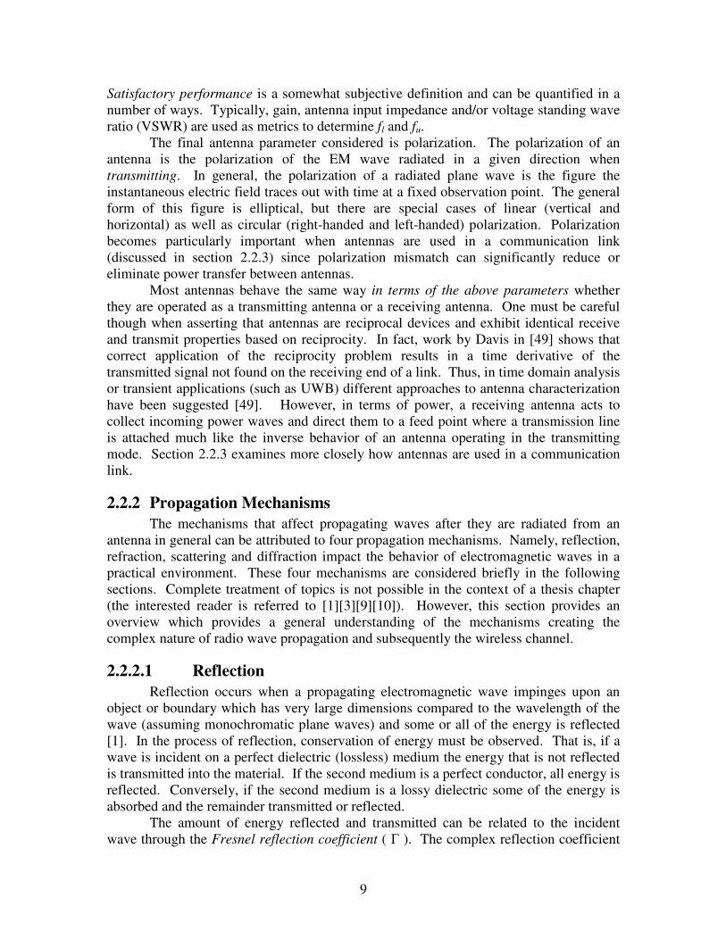
boundaries and describes how signals bend around the obstacle, giving rise to signal energy in regions completely blocked from the source. Typically, Huygens’ principle is used to describe the basic mechanism of diffraction when the obstacle is large compared to the wavelength of the impinging signal [1] [3]. Huygens ’ Principle suggests that each point on a wavefront acts as the source of a secondary spherical wavelet and that these wavelets combine to produce a new wavefront in the direction of propagation [3] as shown in Figure 2.1. Consideration of wavelets originating from all points on XX’ leads to an expression for the field at any point on YY’ in the form of an integral, the solution of which shows that the field at any point of YY’ is exactly the field at the nearest point on XX’, with its phase lagged by 2d/. The waves therefore appear to propagate along straight lines normal to the wavefront as shown from YY’ to ZZ’. These straight lines are known as rays and are typically referred to when discussing multiple propagation paths in communication systems. This explanation assumes that the wavefronts extend to infinity without obstruction and is an idealized case, but serves to describe the propagation of plane waves using Huygens’ Principle.
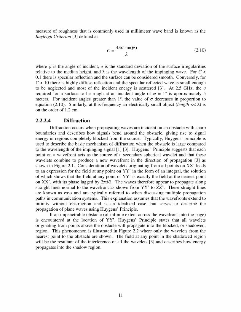
If an impenetrable obstacle (of infinite extent across the wavefront into the page) is encountered at the location of YY’, Huygens’ Principle states that all wavelets originating from points above the obstacle will propagate into the blocked, or shadowed, region. This phenomenon is illustrated in Figure 2.2 where only the wavelets from the nearest point to the obstacle are shown. The field at any point in the shadowed region will be the resultant of the interference of all the wavelets [3] and describes how energy propagates into the shadow region.
λψπσ )sin(4=C
12
Figure 2.1 – Huygens’ Principle applied to the propagation of plane waves in a lossless medium
Figure 2.2 – Huygens’ Principle applied to diffraction at the edge of a sharp obstacle
A concept associated with diffraction which is essential in calculating diffraction loss is the notion of Fresnel Zones. Fresnel zones represent successive regions where secondary waves have a path length from the transmitter to the receiver which are n/2 greater than the total path length of a line-of-sight path [1]. Fresnel zone geometry is illustrated in Figure 2.3. The radius of each successive Fresnel zone is given by
X
X'
Y
Y'
Z
Z'
X'
X
Y' Z'
Y Z
Shadow RegionObstacle
13
(2.11)
where the distances d1 and d2 are much larger than the radius of the Fresnel zone rn and is the wavelength of the signal.
Figure 2.3 – Fresnel zone geometry. Concentric circles define the boundaries of successive Fresnel zones.
Successive Fresnel zones have the effect of alternately providing constructive and destructive interference to the total received signal. If an obstruction is placed in the path of a plane wave (as in Figure 2.2) a blockage of energy will occur and only some of the transmitted energy will reach the receiver location. The reduction of energy can be quantified using parameters, such as the Fresnel-Kirchoff Diffraction Parameter which is presented in [9]. In general if an obstruction does not block the volume contained within the first Fresnel Zone, the diffraction loss will be minimal [1]
Predicting the field strength in the shadow region and estimating diffraction loss has been a topic of extensive research and many models and methods have been proposed, all of which are beyond the scope of this thesis. Many of these models are described in [1] [3] and [9]. In practice, prediction is a combination of theoretical approximation modified by empirical corrections. Although the mathematical problem is complex, some models such as the knife-edge diffraction model, give good insight into the diffraction loss and match measured results.
While propagation mechanisms can give insight into how waves interact with the environment, engineers are usually concerned with how the effects of the environment can be modeled so improvements to systems can be made. Furthermore, any realistic environment becomes analytically difficult to track or model using basic propagation
T
d1
r1
r
0
2
d2
R
1
2
21
21
ddddn
rn += λ
14
mechanisms and simplifying assumptions are usually used. To this end, we first consider the simplest propagation link model.
2.2.3 The Friis Transmission Formula and Basic Communication Link In the previous sections, radiation, antennas and propagation were considered
separately. However, any practical communication system will make use of all of these concepts to facilitate the transfer of information from one location to another. Classically, this problem has been modeled using the Friis transmission formula, which combines the concepts above to provide a single equation estimator for received signal strength at a fixed distance from the transmitter. This section develops the Friis transmission formula and addresses the basic communication link. In this sense we first develop the classic Friis transmission formula, and modify it to include the effects of loss due to a communication system.
As a starting point, the frequency domain received power can be defined in terms of the incident power density S, and the realized effective aperture Aer, or
(2.12)
where S is the same as the radiated power density expression of (2.2). Using equation (2.1) the power density S over a uniform sphere of radius R (in meters) is given by
(2.13)
where Pt is the time average input power accepted by the transmitting antenna. This power density corresponds to an isotropic radiator which distributes the power uniformly in all directions. For the case of a transmitting antenna which is not isotropic, equation (2.13) can be modified to include the effect of the gain using (2.4) resulting in
(2.14)
The numerator of (2.14) is often referred to as the Effective Isotropically Radiated Power or EIRP in the direction of peak gain. It is formally defined as the power gain of a transmitting antenna in a given direction multiplied by the net power accepted by the antenna from the connected transmitter; in (2.14) the directional maximum is assumed. This means to obtain the same radiation intensity with an isotropic antenna, the input power would have to be larger by a factor of Gt. Using equation (2.14) in the expression for received power given by (2.12) gives the available received power as
(2.15)
err SAP =
24 RP
S t
π=
24 RPG
S tt
π=
ertt
r ARPG
P 24π=
15
where again Aer is the realized effective area of the receiving antenna. Using (2.5) the realized effective area of the received antenna can be written in terms of the gain and wavelength of the signal yielding
(2.16)
where the angular maximum gain is assumed for both the transmitter and receiver antenna gains. Combining like terms results in the standard form of the Friis transmission formula [1]
(2.17)
The path loss, which is usually used to determine the loss due to free space propagation, is often quantified as
(2.18)
Path loss is a common metric used to predict signal strength for a receiver located a distance R from the transmitter in communication links. The loss associated with this quantity is due to the reduction of the power density S as the radiating wave propagates further away from the source. Note that the term is due to aperture and assumes gain is constant with This effect is seen from equation (2.13) where for the same input power Pt, the power density S decreases as R increases (for the isotropic case). From equation (2.18) it is evident that doubling the distance will cause the path loss to increase by a factor of 4 (6 dB), which is known as the free space path loss. Path loss as a channel parameter and its dependence on the environment is discussed in Section 2.3.4.
Equation (2.17) deals in terms of power accepted by the transmitting antenna and power available at the receiving antenna. These powers include the losses due to dissipation on the antennas (radiation efficiency contained in the gain expression) but only the transmit power Pt includes the power loss due to impedance mismatch since it is designated as power accepted by the transmitting antenna. When the receive antenna is connected to a transmission line for use in a communication system receiver, power loss will occur unless it is perfectly impedance matched. From a lumped circuits standpoint, the power delivered to a load with impedance ZL = RL + jXL from an antenna with impedance ZA = RA + jXA is given by [8]
(2.19)
2
24 4t t r
r
G P GP
Rλ
π π=
2
2
)4( RGG
PP rttr π
λ=
2
4
=R
PLπλ
LLALA
LAD RXXRR
VRIP 22
22
)()(||
21
||21
+++==
16
where V is the open circuit voltage across the antenna terminals. Maximum power will be transferred to the load when a conjugate impedance match exists, or (RL = RA and XL = -XA) or the impedance is purely real (XA=XL=0 and RA=RL) In the case of a normal transmission line, the impedance is almost always real thus maximum power transfer is rarely achieved. The fraction of power delivered is known as the impedance mismatch factor and is given by the ratio of delivered power and maximum available power [8] or
(2.20)
where 0 < q < 1. The impedance mismatch factor can also be computed from the complex reflection coefficient (usually obtained from an s11 s-parameter measurement on a network analyzer) if the input impedance is not explicitly known using the relation
(2.21)
where is the field reflection coefficient, defined by equation (2.9). Therefore, including the effects of impedance mismatch the power delivered to the transmission line is PD = qPr where Pr is defined by (2.17).
Additional losses in the received power can occur if the transmitter and receiver antennas are not matched in polarization. To account for polarization mismatch, a polarization efficiency factor p is defined which takes values from 0 to 1. A complete mismatch (p = 0) occurs when the incident wave and antenna are cross-polarized; for example, orthogonal linear states, such as horizontal and vertical polarizations or right-hand and left-hand polarization. Including the effect of polarization efficiency the delivered power is given by
(2.22)
where pt and qr represent the polarization loss at the transmitter and impedance mismatch at the receiver respectively. The polarization efficiency is typically near 1 in a measurement application since matched antennas are usually used. However, if the signal propagates through a medium that causes depolarization, the efficiency may be reduced. A complete treatment of polarization efficiency and methods for calculating it can be found in [8]. Equation (2.22) also assumes the antennas are aligned for maximum gain. If not, the directional properties of the gain must be included to obtain an accurate estimate of the received power.
Finally, the bandwidth of both the transmit and receive antennas should be larger than the bandwidth of the transferred signal to avoid signal distortion. Furthermore, for narrowband systems, the properties of the antenna usually do not change significantly over the occupied bandwidth. However, for spread spectrum or UWB applications, the antenna parameters may vary significantly over the occupied band, which should be accounted for in the link [49].
22 )()(4
LALA
LA
XXRRRR
q+++
=
2||1 Γ−=q
2
2(4 )t r
D r t r t
G GP pqP p q P
Rλ
π= =
17
2.3 The Indoor Propagation Channel The Friis transmission formula, adjusted for losses due to the system, is only
accurate in predicting received signal strength when the transmitter and receiver have a clear, unobstructed line-of-sight path between them. Typical indoor links cannot be described by the free space propagation formula since the signals undergo reflection, scattering, and diffraction causing multiple paths to arrive at the receiver. These multiple paths, known as multipath combine at the receiver to form a distorted version of the original signal, seriously degrading the performance of communication systems [4]. However, if the multipath structure is well characterized, systems can be designed to mitigate the effects of multipath, thus improving performance. Detailed characterization of the indoor channel is therefore essential for deployment of successful indoor systems.
Due to the complexity of wireless channels, models have historically been used by communication engineers to characterize the distortion caused during transmission. Furthermore, these models have been broken into micro and macroscopic effects for more detailed analysis. Statistical models are based on extensive measurements which are usually applicable to the environments in which the measurements were taken. One widely used example is the Saleh-Valenzuela model derived from numerous indoor measurements. Yet other models rely on physics and the principles of electromagnetic (EM) field interaction, a deterministic approach, in an attempt to predict the nature of the propagating EM waves between the transmitter and receiver. Ray tracing and diffraction models fit into this category [3]. Some models, such as the classic Clark-Gans fading model use a combination of both to describe the complex nature of the transmission channel [1].
In this section we first consider how the indoor channel is modeled in both a macro and microscopic sense to account for the existence of multiple propagation paths. Next, the specific impact of multipath in communication systems is examined by presenting some of the parameters used to characterize multipath channels. The final section presents a survey of work in the area of bandwidth vs. system performance analysis that is pertinent to this research effort.
In order to compare different multipath channels and to develop general design guidelines for wireless systems, parameters which quantify the multipath channel are used [1]. In this section these parameters are presented and quantified as either large scale or small scale fading effects, both of which are defined below.
2.3.1 Large Scale Effects
Large Scale propagation effects are used to describe the variation in signal strength over large transmitter-receiver distances (tens of wavelengths) primarily due to the spreading loss (or path loss) described in Section 2.2.3. The path loss exponent gives a measure of the rate at which the path loss increases with distance in a particular environment and is a useful tool in characterizing indoor environments. Large scale effects are typified by the macroscopic view of the channel, providing information on coverage area, signal to noise ratio (SNR), and possibly optimum locations for base station antennas [4]. Large scale effects are modeled on data that does not include local area variation due to multipath (small scale effects) and is usually collected from an average of many measurements in a local area. There have been many path loss models
18
reported for the indoor channel in the literature [4] yet one of the most common is the log-distance path loss model, which indicates the average received signal power decreases logarithmically with distance or
(2.23)
where )(dPL denotes the average of all possible path loss values for a given T-R separation distance d, n is the path loss exponent, and d0 is a close-in reference distance (typically 1m for indoor measurements). The average received power can be modeled as [33]
(2.24)
where )( 0dPr is the average received power at the reference distance including the effects of the antennas and is usually assumed to be a free space reference. The reference can be calculated using the Friis transmission formula if the antenna gains and system losses are known using equation (2.22). When measuring )( 0dPr it is assumed the spatial averaging over a local area will mitigate the effects of multipath and the reference is relative to free space [1]. It should be noted however, some researchers do not use free space and may include multipath in their reference measurements. Path loss can be calculated for subsequent measurements using the reference distance as
(2.25)
Combining equations (2.24) and (2.25) gives the expression for path loss in terms of the path loss exponent n, and distances d and d0 as
(2.26)
this can be expressed in decibel units as
(2.27)
Using (2.25) and (2.27) allows n to be determined from a set of measurements where the received power is measured for various T-R separation distances d.
The path loss for two different locations having the same T-R separation can vary significantly depending on the intervening channel structure. These variations, known as
n
dd
dPL
∝
0
)(
n
rr dd
dPdP
=
00 )()(
)()(
)( 0
dPdP
dPLr
r=
n
dd
dPL−
=
0
)(
−=
010log10)(
dd
ndPL dB
19
shadowing, have shown to be log-normally distributed and the path loss equation of (2.27) can be represented by
(2.28)
where X is a zero-mean Gaussian distributed random variable (in dB) with standard deviation to include the effects of shadowing [1]. It is noted that the primary mechanism responsible for shadowing is diffraction in the indoor propagation channel. Equations (2.27) and (2.28) can also be written in terms of Pr using the relation Pr(d) = Pr(d0) – PL(d), all in dB. An estimate for the path loss exponent is obtained by finding the least squares estimate from the measurement points [1]. A number of path loss exponents have been reported in the literature for the indoor propagation environment, ranging from as low as 1.3 [33] for LOS hallway measurements in a university building to 5.2 [1] for propagation through multiple floors in another university building. Path loss in hallways and corridors is frequently reported less than free space and is usually attributed to the wave guiding effect of the corridor on the propagating waves. Several other indoor path loss models have been suggested for the indoor channel which takes into account the number and type of obstacles present in the path. These models sometimes referred to as attenuation factor [1] or partition based [5] path loss models make use of extensive data bases of loss factors for different types of materials to predict the received signal strength. For a complete treatment of these models, the reader is referred to [1].
2.3.2 Small Scale Effects Small scale fading effects are characterized by the rapid fluctuations of a received
signal over a local area (several wavelengths) due to the interaction of multiple paths arriving at the receiver with slightly different amplitudes, time delays, and phases. The effect of small scale fading can cause the received signal to vary significantly between points close in space, in some cases by three or four orders of magnitude. Fading can be characterized statistically from the distribution of received power values in a local area. For a real random variable with known probability density function (PDF) the fading variance is given by
(2.29)
where x is a real random variable with a known PDF and E[x] = is the expected value or mean of x. In many cases the underlying distribution is not known, in which case the sample variance can be estimated from N independent samples using (2.30)
(2.30)
2222 ])[(][)][( xExExEx −=−= µσ
2 2
1
1( )
1
N
x i xi
xN
σ µ=
= −−
σXdd
ndPL dB +
−=
010log10)(
20
where µ is the sample mean for the data set. Strictly speaking this formulation must be used since for an unknown set of data the mean in not explicitly known and only an estimate of the mean is used [34]. Before proceeding with a discussion of the small scale fading parameters, the mathematical model and typical characterization of the propagation channel impulse response is considered.
2.3.2.1 Mathematical Modeling A generally cited model for the indoor propagation channel is based on the form
of the impulse response of a linear time-varying filter [1] [3] [4]. Many reported statistical models are derived from this formulation. For each point in three dimensional space the channel is a linear time-varying filter with the impulse response given by:
(2.31)
where t and are the application time (of the impulse) and observation time (excess delay), respectively, N(t) is the number of multipath components, ak(t,), k(t),k(t,) are the random time-varying, amplitude, arrival time, and phase values of the kth multipath, respectively and is the delta function [4]. Note that in this definition all phase shifts are lumped into the single variable k(t,) which represents phase shift due to free space propagation as well as any additional phase shifts that are encountered in the channel. Under this complex baseband model the small scale channel is completely characterized by these path variables.
A specialized case of this model, the time-invariant version, assumes that the response of the channel is static over some fixed observation time and does not vary relative to the application time of the impulse. For this stationary model equation (2.31) reduces to
(2.32)
This model assumes that the channel impulse response is at least wide sense stationary (WSS) or the first and second moments are independent of time. Research has shown that the indoor channel is rarely time-invariant [4] but can be modeled as such under many circumstances.
A further extension of this model is the discrete-time impulse response model, which can be applied to either the time-variant or invariant case [3]. In this model the time axis of equation (2.32) is divided into small time intervals known as delay bins having a fixed width . In this model each bin is assumed to contain either one multipath component or no multipath component with the possibility of more than one path per bin excluded [1]. For convention, 0 = 0 (time of the first arriving component), 1 = , t2 = 2, and in general k = k. The size of the delay bins determines the time delay resolution of the model; therefore a reasonable bin size is the resolution of the specific measurements (if the model is measurement based) [3]. An example of a
),(1)(
0
)]([),(),( τθττδττ tjk
tN
kk
kettath −= −
=
kjk
N
kk eah θττδτ )()(
1
0
−=−
=
21
discrete-time impulse response model is shown for both a time-variant and time-invariant channel in Figure 2.4.
Figure 2.4 – Examples of time varying (left) and time invariant (right) discrete time channel impulse responses.
It is important to note that depending on the choice of and the physical delay properties of the channel, there may be two or more multipath signals that arrive within any given delay bin that are unresolvable. Unresolvable multipath components combine vectorially to yield the instantaneous amplitude and phase of a single modeled component [1]. Known as fading this situation causes the multipath amplitude within the bin to vary over a local area (on the order of a few wavelengths) according to the vector sum. Fading is discussed in detail in Section 2.3.3.
The channel impulse response model is sometimes modified to include angle-of-arrival (AOA) statistics in addition to the time-of-arrival (TOA) statistics for each multipath component. Systems that use spatial filtering, diversity, or beamforming, can use this information to help mitigate the effects of multipath [1].
There are a multitude of models that characterize the arrival time, AOA, multipath amplitude and phase values of the channel impulse response. Even a broad overview of these models is beyond the scope of this thesis. However, the parameters from a large number of models as reported and collected from references [1] [3] [4] [33] [35] and [36] are summarized in the list below (adapted from [36]).
1. Distribution of arrival times k have been reported to follow:
a. Standard Poisson Model [4] [33]
b. Modified Poisson – The -K Model [4] [33] [35]
c. Modified Poisson – Weibull Interarrivals Model [4]
d. Double Poisson (Saleh-Valenzuela / Neyman-Scott Model) [1] [4] [33]
2. Distribution of angle-of-arrival (AOA) have been reported as:
(t 0
h(t, )
0t
Time Varying Discrete-Time Impulse Response Time Invariant Discrete-Time Impulse Response
0
t
t1
t2
1 2 3 4 5
)
)(t 1
(t )2
(t )
t0
0
)(t 1 2 3 4 5
0
t1
t2
1
h(t, )
t
2)(t
22
a. Uniformly distributed over [0,2) [1]
b. Clustered – calculated/measured for the specific environment [3]
3. Distribution of path amplitudes ak have been reported to follow:
a. Rayleigh Distribution [1] [3] [4]
b. Rician Distribution [4]
c. Nakagami Distribution (m-distribution) [4]
d. Weibull Distribution [4]
e. Log-normal Distribution [4]
f. Suzuki Distribution [4]
Where in general, the distribution used to model the relative average
values of the successive multipath component powers is an
exponential decay (for all listed distributions) [36].
4. The multipath phases have been reported to be:
a. Uniformly Distributed over [0,2) for the initial phase [1] [4]
b. Incremented by:
i. Random Variable (Gaussian) [4] [36]
ii. Deterministic value calculated from the environment [36] [4]
The literature shows that all of these models have generally shown good fit to measured data for some indoor channels [4] with the exception of the standard Poisson model, which has proved inaccurate for a large number of measurements [1][4]. The multitude of channel models and their limited application suggests that the channel’s parameters have great dependence on the shape, size, and construction of the particular building of interest.
The statistics for channel impulse responses for points that are located closely in space exhibit some degree of correlation [4][33]. This is expected since principle reflectors and scatters causing the multipath structure may remain the same over a short distance. The degree of correlation is therefore dependent on the structure of the channel (particularly multipath angular spread) and the separation distance between profiles, as well as the antenna response [3]. Spatial correlation statistics are important since they may provide information for diversity techniques in receiver design [3]. Spatial correlation is examined in more detail in Section 2.4 as well as in Chapter 6
By definition the power delay profile is the magnitude squared of the channel impulse response given by |h()|2. Depending on the intended application, power delay profiles can be averaged to produce a single local area estimate or considered separately to examine small-scale local area channel states [1].
23
In many cases the channel impulse response is measured or predicted by exciting the channel with a probing pulse s(t) that approximates a delta function [1] [6]. By definition the signal at the receiver w(t) is the convolution of the channel impulse response and the probing pulse s(t) given by
(2.33)
where ⊗ denotes convolution and is the variable of convolution. The channel impulse response can be extracted using deconvolution techniques or predicted by the received signal w(t) without deconvolution under certain conditions. In general, the probing pulse does not need to be deconvolved from the measured response if it has time duration much shorter than the impulse response of the multipath channel [6]. If this is the case the received power delay profile is given by
(2.34)
where Po is a proportionality constant that relates the transmitted power in the probing pulse s(t) to the total power received in a multipath delay profile [1]. Chapter 3 discusses obtaining the channel impulse response and multipath information using the sliding correlator measurement technique.
To ease the analysis of bandpass signals or signals modulated onto a carrier, the complex baseband or complex envelope representation is used [26]. A general bandpass signal can be written in the form
(2.35)
where A(t) is the time varying amplitude and ( )tφ is the phase deviation from the phase 2fct where fc is generally taken as the carrier frequency of the modulated signal. By definition the complex envelope is given by [26]
(2.36)
Conversely, the general bandpass signal can be obtained from the complex envelope by
∞
∞−
−=⊗= ζζτζτ dhshtstw )()()()()(
2|)(|)( ττ hPP O=
)](2cos[)()( ttftAtx c φπ +=
)](exp[)()(~ tjtAtx φ=
24
(2.37)
The complex envelope representation has the effect of removing high frequency variations caused by the carrier, making the signal analytically easier to handle [1]. It follows that the response of the bandpass channel given by (2.33) at baseband (or in complex envelope representation) is
(2.38)
where )(~ tw and )(~ ts represent the complex envelope representation of the received signal and probing pulse, respectively. The ½ factor relating the channel impulse response to its complex envelope is due to the properties of the complex envelope as shown by Couch in [27]. We now return our attention to the small scale parameters that are used to characterize multipath fading channels.
2.3.2.3 Small Scale Fading Parameters The fade margin is a system parameter that is built into link budgets to account
for small scale fading. That is, a certain amount of power over the minimum required value is built into the system link budget to ensure system operation even during fades. In addition to the fading variance, several parameters have been developed to quantify the effect of time dispersion as well as fading. Namely, the mean excess delay, RMS delay spread, and maximum excess delay (X dB) are time dispersion parameters that characterize the wideband indoor channel.
The mean excess delay, m is the first moment of the power delay profile and is defined as
where 2ka and k are the multipath amplitude and arrival time of the kth
multipath component and P() is either an average or single power delay profile [1]. Similarly, the RMS delay spread is the square root of the second central moment of the power delay profile defined as [1]
(2.40)
The delay values k for both the mean excess delay and RMS delay spread are measured relative to the first arriving component 0 as is the convention of the discrete time channel
−=
−=
kk
kkmk
kk
kkmk
RMS P
P
a
a
)(
)()()( 2
2
22
τ
ττττττ
==
kk
kkk
kk
kkk
m P
P
a
a
)(
)(
2
2
τ
ττττ (2.39)
]2exp[)(~Re)( tfjtxtx cπ=
1
0
1 1( ) ( ) ( ) ( ) ( ) ( ) [ ]
2 2k
Nj
k kk
w t s t h s t h s t a e θτ τ δ τ τ−
=
= ⊗ = ⊗ = ⊗ −
25
impulse response. RMSτ (also denoted by in some texts [1]) is a measure of multipath spread and has been shown to be a good predictor of the maximum achievable data rate through channels without equalization [1]. The excess delay spread (X dB) is defined to be the time delay during which the multipath energy falls to X dB below power of the strongest multipath component. In essence, the maximum excess delay spread defines the extent of multipath energy above the X dB threshold. The values for mτ and RMSτ depend on the choice of the noise threshold used to process the power delay profile. If the threshold is chosen too low, noise is processed as multipath causing mτ and RMSτ to appear artificially high. Conversely, if the threshold is set too high, significant multipath components can be missed giving underestimates to the true RMS and excess delay spreads [1]. The impact of threshold level on time dispersion parameters is shown in [11]. In the indoor channel, measurements show that excess delay and RMS delay spread depend on the size and type of the building, existence or absence of a clear LOS path and obstacles in the propagation path. Typical values have been reported from 20 and 50 ns for small and medium size rooms up to 200 ns for large office buildings [4]. It has also been reported in [4] that a number of researchers have found correlation between
RMSτ and T-R separation distance. A useful parameter derived from the RMS delay spread is the coherence
bandwidth of the channel which is a statistical measure of the range of frequencies over which the channel can be expected to pass all spectral components with equal amplitude and linear phase [1]. The coherence bandwidth provides a metric for how highly correlated two frequency components are in amplitude. The coherence bandwidth can be approximated by [1]
(2.41)
where the Bc is the bandwidth over which the frequency correlation function (as defined in [1] and [5]) is above 0.9. A similar definition with the correlation requirement relaxed is given by
(2.42)
where Bc is the bandwidth over which the frequency correlation between spectral components is above 0.5. In both cases, the coherence bandwidth is an estimate based on empirical results [1]. In general, spectral analysis techniques and simulation are required to determine the exact impact the time dispersive multipath has on a particular transmitted signal [1]. However, the coherence bandwidth provides a metric to estimate whether a signal will undergo flat or frequency selective fading which can affect the performance of a communication system.
RMSCB
τ501=
RMSCB
τ51=
26
For flat fading channels, the bandwidth of the transmitted signal BRF is much less than the coherence bandwidth Bc, such that the entire transmitted signal will undergo similar amplitude variations as the channel gain varies over time. This type of fading is typified by narrowband systems, causing deep fades of several orders of magnitude. Although the signal may fade significantly, the effect is that the channel may be modeled as having no excess delay and only a single component [1]. Conversely, for frequency selective fading channels the bandwidth of the transmitted signal is greater than the coherence bandwidth of the channel causing the received spectrum to exhibit variations in gain and phase. In this scenario, the received signal includes multiple versions or the transmitted waveform which are attenuated and delayed. Frequency selective fading channels are typified by wideband systems where the signal spectrum spans several coherence bandwidths. Frequency selective fading channels are much more difficult to model than flat fading channels since each multipath component must be modeled and the channel must be considered a linear filter as in the model of (2.24). This is evident from the definition of the coherence bandwidth which gives a measure of how correlated spectral components are. In general there is also degradation due to relative motion between the receiver and motion of objects in the channel. This motion causes spectral broadening due to motion as well as a time variant channel due to the surrounding environment changing relative to time. These effects are well characterized as in [1] and [3], but are not of interest to this study since there is no relative T-R motion and the channel is assumed stationary over the observation time. The stationary channel assumption is valid since all measurements are taken late at night with no motion in the channel.
2.3.2.4 Multipath Fading and Signal Bandwidth Relationship – A 2 Path Model
To illustrate multipath fading and its dependence on bandwidth, we first consider two cases of signals propagating in an identical multipath environment and then generalize the result. The first case is the scenario of transmitting an unmodulated carrier of normalized amplitude 2 through a two path (line of sight and single multipath reflection) propagation channel. The second case is transmitting a pulse train p(t) of very narrow pulses through the exact same channel. These scenarios represent exciting the channel with both a narrowband and wideband signal and will be used to demonstrate the impact signal bandwidth has on fading. For both cases considered, we assume a time-invariant channel.
First, the complex envelope of the unmodulated carrier is given by )(~ ts = 2. From equation (2.38) the instantaneous complex envelope of the received signal is given by
(2.43)
where ak and k represent the real amplitude and phase of the two paths in the channel, respectively. The corresponding instantaneous power is given by the magnitude squared of the complex envelope as
kj
kk eatw θ
=
=1
0
)(~
27
(2.44)
Equation (2.44) illustrates an important result. First, if we consider the case where the two signals arrive with equal amplitude and are 180° out of phase, the received power goes to zero. Conversely, if the signals are in phase the received power is four times the power contained in the first arriving path a0. This phenomenon is the mechanism which causes fading in the received power envelope of narrowband communication systems. The phases of the incoming components are dependent upon the distance traveled by the wave as well as the other mechanisms which induce phase shifts (such as reflection). Over a local area the phase can vary widely. Consider the case of an unmodulated carrier at 2.5 GHz; the phase will shift 180° for every 6 cm traveled. In reality, the limiting cases of zero power and quadruple power never occur but this type of severe fading typifies the behavior of CW and narrowband signals. The second case considered is the scenario of transmitting a repetitive pulse train p(t) with very narrow pulse width Tbb and repetition period TREP which is much greater than the maximum measured excess delay MAX. Again using equation (2.38) the low pass channel output is found by convolving the pulse train with the channel impulse response and yields
(2.45)
where the a single pulse of the pulse train is defined as
(2.46)
To determine the instantaneous received power received at some time t0, the power 2
0 |)(~| tw is found by summing up the multipath powers resolved in the instantaneous
multipath power delay profile of the channel 20 |);(| τth . This is equal to the energy
received over the time duration of the multipath waveform, divided by the duration of the waveform MAX [1]. As shown in Appendix B, the instantaneous received power is given by
)(21
)(~1
0k
j
kk tpeatw k τθ −=
=
bb
MAX
Ttp
τ2)( = for 0 t Tbb
0)( =tp otherwise
21
0
2 |||)(~| kj
kk eatw θ
=
=
210 || 10 θθ jj eaea +=
)cos(2 10102
12
0 θθ −++= aaaa
)cos(2 1010
1
0
2 θθ −+==
aaak
k
28
(2.47)
where ak is the multipath amplitude, k is the multipath arrival time, k is the multipath phase, and Rp() is the autocorrelation function of the probing pulse, given by (2.46).
If |1 – 0| > Tbb, then Rp() = 0, and the two paths are resolved unambiguously reducing (2.47) to only the first term. That is, the instantaneous received power is reduced to the sum of the powers of the individual multipath components. However, if |1 – 0| < Tbb the paths are not completely resolved and the contribution of the second term of (2.47) depends on relative difference in the multipath phases and the value of the autocorrelation function at = (1 – 0), where for square pulses
(2.48)
From the definition of the autocorrelation function, it is evident that the magnitude of the second term in (2.47) will be maximized when the two components arrive with identical delay corresponding to Rp(0), and decrease as the arrival times become further spaced in time, until they are completely resolved, provided 1=0. Conversely, when the width of the probing pulse Tbb is decreased, the delay for which complete resolution occurs also decreases. In the limit as p(t) (t), Tbb 0, and all of the paths of the channel are resolved provided they do not arrive at exactly the same delay k.
Equation (2.44) and (2.47) also illustrate that the received local ensemble average power (over a small scale region of distances) of wideband and narrowband signals are equivalent under certain conditions. If either the multipath phases are IID uniform over 2 or the path amplitudes are uncorrelated, the second terms of (2.43) and (2.47) become zero[1]. Namely, if 0)cos( 10 =−θθ and/or 0][ 10 =aaE , the result of (2.44) and (2.47) are identical, where the overbar denotes ensemble average [1].
Both the narrowband and wideband examples have frequency domain equivalents related by the Fourier transform. To illustrate this, we simplify the wideband case of (2.43) by assigning 0 = 0 where 1 0, and assuming p(t) can be approximated by a delta function, this simplification yields an expression of the form
(2.49)
)]()([21
)('~110 τδδ −+= tststw
)()cos()()(2)(|)(~| 01100100
1
00
220 ττθθ −−+=
=p
kk Rtatatatw
=)(τpR
-Tbb 0
|| > Tbb
0 < Tbb bb
MAX
Tτ
4
+ 1
bbTτ
+−
1bbTτ
0
29
Where s0 and s1 are complex coefficients representing the amplitude and phase of the two arriving components. Applying the Fourier transform yields an expression that is proportional to the spectrum of the received signal given by
(2.50)
where K is a proportionality constant. Equation (2.50) shows that changing the delay time 1 will result in a change in the frequency response of the channel. Extending the model of (2.50) to include multiple paths will result in an increasingly complex frequency response which in turn, can cause frequency selective effects. This illustrates the basic concept behind the coherence bandwidth definition presented in the previous section. That is small implies are large coherence bandwidth, and large implies a small coherence bandwidth.
From this discussion it is clear that for the 2-path model the fading in the received power is a function of the pulse width Tbb of the probing pulse and the delay between the two multipath components. While this discussion only considered a two ray model, the derivation can be extended to the case where N multipath components are present [1]. For the general case the fading is a function of the interarrival times (similarly, the RMS delay spread) of the multipath components, which is a function of the propagation environment [4]. It is possible that some multipath components will be resolved while others will not resulting in a complex relationship between fading and probing pulse duration. On the average, it is expected that for a fixed channel, the amount of fading will decrease as the pulse width is decreased. From a frequency domain perspective, as the bandwidth of the probing pulse increases the severity of fading is expected to decrease.
From a communication system standpoint, it is also evident a trade-off may exist between the bandwidth of a message signal and system complexity. Specifically, for a channel with a fixed coherence bandwidth the fading will vary from flat fading to frequency selective fading as the transmitted signal bandwidth is increased from narrowband to wideband, where it is assumed the desired data rate can be achieved using the lowest transmission bandwidth, which is the case in many spread spectrum systems. From a complexity standpoint, a receiver that tracks only one path (as in the flat fading case) will be simpler than a receiver that must track multiple paths (as in the frequency selective case) to recover the same amount of energy. However, the simpler receiver will have to cope with the deep fades (possibly requiring a larger fade margin to maintain satisfactory performance) while the more complex implementation may be able to combine the paths for a net advantage. This illustrates one of the fundamental trade-offs between bandwidth and system complexity for indoor systems.
The main question becomes can one quantify the tradeoff between bandwidth and system performance for indoor wireless systems. As described in Chapter 1 this issue is one of the main focuses of this research. Through an extensive measurement campaign and channel analysis using the above techniques this question is addressed in this thesis as shown in Chapters 5 and 6. A second, perhaps not so obvious question is can this trade-off be addressed by processing a single high resolution measurement, which is now briefly addressed and revisited in Chapter 3.
]]2exp[[)('~
110 τπfjSSKfW +=
30
With a few exceptions as noted, the channel parameters discussed in the previous sections have been investigated by sounding the channel with one distinct pulse shape (for the case of pulse or pulse compression measurements) or frequency step (for the case of swept frequency measurements) to extract the channel impulse response of the channel. In theory, convolution of the impulse response with an information signal (such as one used in a communication system) will yield the received signal when transmitted through the channel [1]. Similarly, filtering of the frequency spectrum of the channel transfer function H(f) can yield the response corresponding to various time resolutions. In essence, only one channel measurement in the desired portion of the radio spectrum is required to predict the response of the channel as a function of signal bandwidth.
However, there is no known evidence in the literature which compares actual measured responses generated from various pulse widths to analytical results obtained through convolution or filtering. Furthermore, a swept frequency measurement is limited by the total number of frequency steps and their spacing. For very large bandwidth sweeps, the measurement resolution will be limited by the number of frequency points.
The lack of evidence supporting the processing of high resolution measurements to predict narrowband responses as well as the limitations of frequency swept methods motivate a study to investigate these claims. Therefore, this thesis takes the approach of conducting identical collocated measurements with different bandwidth sounding pulses (using the sliding correlator technique) rather than processing one high resolution measurement per location. The specific tradeoff between the frequency swept and sliding correlator methods are addressed in detail in Chapter 3.
2.4 Multipath Mitigation Techniques The discussion of the previous sections of this chapter have both motivated and illustrated the negative effects of multipath propagation in communication systems. Since multipath has proven to be one of the most detrimental influences on communication system performance, many techniques have been devised to address it. These techniques, commonly referred to as multipath mitigation techniques are briefly considered in this section, with emphasis place on Rake receivers. The Rake receiver is considered since it is the receiver structure considered in depth in Chapter 6.
2.4.1 Basic Diversity Methods One well known method of reducing the effects of fading is to use diversity reception. The basic principle of diversity is the notion that two or more samples of the incoming signal will have low, ideally zero, cross-correlation. Basic statistics state that the probability of M independent samples of a random process all being simultaneously below a certain level is pM
where p is the probability that a single sample is below the level. It can be seen that a signal comprised of a suitable combination of multiple signals will have a lower probability of falling below the certain level, and exhibit less severe fading properties [3]. While there are many forms of diversity (such as polarization, frequency and field) we will focus on spatial and temporal diversity for this discussion.
For the spatial diversity discussion we will assume that there are M available versions of the signal at the receiver. Whether these signals came from multiple antenna
31
elements or other methods is left generalized for the time being. In general there are three methods for processing these signals. Known as linear combiners they are selection diversity, maximal ratio combining, and equal gain combining. Under a certain set of assumptions, the output of these combiners stot(t) can be represented by a weighted sum of the M input signals sk(t) given by
(2.51) given that (1) the noise in each branch is independent of the signal and is additive (2) the signals are locally coherent (3) the noise components are locally incoherent and have zero means, with constant power and (4) the local mean squares of the signals are statistically independent (uncorrelated) [3]. Different realizations and performance is obtained based on the choice of the ak values which is discussed briefly here. For selection diversity, a single ak corresponding to a single branch of the M total branches is unity and the other ak coefficents are zero. In this sense, the receiver logic selects the path with the highest instantaneous SNR and uses it as the received signal. This is the ideal case, and in practice there are several methods used to choose the best branch such as scanning, which are not discussed here. Although this is one of the simplest forms of diversity, it is also one of the least effective when multiple versions of the signal are available. Maximal ratio combining and equal gain combining both use more than one path in two distinct ways. In maximal ratio combining each branch signal is weighted (by ak) in proportion to its own signal voltage/noise power before summation, which if done before demodulation requires co-phasing of the signals. Conversely, equal gain combining does not weight each signal before combining (all ak = 1). In general, maximal ratio combining provides the best performance gain, followed by equal gain combining and selection diversity for the same number of paths in a Rayleigh fading environment. However, the performance gain comes at the expense and complexity of the weighting amplifiers for maximal ratio combining. Specific improvements from diversity and implementations have been addressed in [2] as well as [1][3].
2.4.2 The Rake Receiver – An Overview The Rake receiver, first proposed by Price and Green, is a spread spectrum receiver that is able to track and demodulate resolvable multipath components, which are sufficiently separated in time [3]. As described in Chapter 1, CDMA systems make use of spreading codes with low cross-correlation when the codes are not synchronized, thus multipath components arriving with delay greater than the duration of one chip in the spreading codes will have low cross-correlation and essentially appear as noise. The Rake receiver architecture exploits this phenomenon by using a number of correlation receivers followed by weighting amplifiers to isolate and demodulate the strongest multipath components. In general, the first correlator is synchronized to the strongest multipath component, followed by the second strongest component synchronized to the second correlator, and the remaining M correlators (or fingers) synchronized to later components. The outputs of the M correlators are weighted to form an overall decision
1
( ) ( )M
tot k kk
s t a s t=
=
32
where the weights can be chosen to produce the equivalent result of maximal ratio or equal-gain combining.
The advantage of the Rake receiver is that if the output of one of the correlators is corrupted by fading, the others may not be, and the corrupted path can be weighted out. This provides an advantage relative to a single correlation receiver, which when synchronized to a single component can suffer from reduced performance (higher BER) if that component undergoes fading.
The ideal Rake receiver (one with unlimited fingers and perfect synchronization to all multipath components) can estimate all multipath components impinging upon the receiver and capture 100% of the available power in all of the multipath components without the use of channel estimation to track the paths. However, in practice this is not possible and some means of estimating the channel must be used.
Therefore the design of a practical Rake receiver is influenced by several factors. From a performance standpoint, a certain amount of power must be dedicated to finding and tracking the multipath components for synchronization with each correlator. This leads to the notion of pilot tones to estimate the channel response. Secondly, components with low SNR relative to the strongest path (10 – 20 dB below) may be harder to track and contribute little to the overall SNR. At some point, paths significantly below the peak will be discarded due to their burden on the system in terms of power consumption. Intuitively, the complexity and cost, both financially and in implementation, increases with the number of fingers. Thus the performance of the Rake receiver is largely based on the number of fingers, the number of multipath components, their amplitude statistics, and the relative SNR of each component tracked.
In Chapter 6 we will examine this tradeoff in more detail for both the ideal Rake receiver, as well as a practical Rake receiver which accounts for channel estimation. For a complete discussion on Rake receivers the reader is referred to [2].
2.5 Impact of Signal Bandwidth on Indoor Wireless Systems – Literature Review
The trade-off between system/receiver performance and signal bandwidth has
received notable attention in the literature, lately in the context of UWB systems, as evident from references [12] [20] [21] [33] [36] – [40] and previously in the context of direct sequence spread spectrum (DS-SS) communication systems as in [3] [41]-[47]. Both large and small scale fading effects have been investigated; however, the majority of this work has focused on small scale fading effects. From a system standpoint, most of the literature focuses on the performance of Rake receivers.
A survey of the literature shows little treatment of path loss as a function of bandwidth except for [33]. In this work the authors calculated path loss for several bandwidth bins of over 1200 UWB pulse measurements, occupying a bandwidth in excess of 10 GHz. The first scenario considered 10 different bins each having 1 GHz bandwidth spread over the entire 10 GHz frequency range. For this case, the path loss exponents were shown to be fairly flat (constant) with some possible frequency dependence for the case of NLOS measurements with an omnidirectional bicone antenna.
33
The second scenario calculated path loss exponents for frequency bins centered around 6 GHz with initial bandwidth of 500 MHz and increasing to 10 GHz. This analysis showed constant path loss exponents for all frequencies and a decrease in the Gaussian shadowing term with an increase in frequency. In general, the conclusion of the report was that there is no frequency dependence introduced by the channel, and that frequency dependence is caused by the antennas. The report however suggested a possible frequency dependence of NLOS channels at large T-R distances due to the frequency dependence of many materials in the propagation path. To the author’s knowledge, aside from this work, there are no reported results which directly examine path loss as a function of frequency. There is however, a larger body of work focusing on small scale fading as a function of bandwidth.
Perhaps the seminal work in this area began with the work of Amoroso and Jones [43] which derived a simulation model demonstrating a variation in the received power envelope as a function of chip duration for Rayleigh fading in a direct sequence spread spectrum system. In the simulation, an ideal raised root cosine (RRC) chip shape was transmitted through a radially uniform field of dense scatterers known to exhibit Rayleigh fading for the case of an unmodualted carrier. The standard deviation of the normalized received power of a single chip was calculated for different chip durations. Subsequent simulations yielded a curve which showed a decrease in standard deviation as chip duration was decreased. For very long chips (narrow spread bandwidth) the standard deviation was shown to approach the 5.57 dB limit for pure Rayleigh fading. The simulation also showed that for very short chips (large spread bandwidths) the standard deviation tended toward zero, but at a decreasing rate, never actually reaching zero for the simulation cases investigated.
Holtzman and Jalloul [44] extended the analysis and derived the coefficient of variation of the received signal power under the same assumptions of [43]. This analysis showed that the relationship is given by a double integral involving the transmitted power spectral density U( ), the pseudonoise chip period T, and the RMS delay spread of the channel, RMSτ . Specifically, the normalized coefficient of variation )|)((| 2tsnσ , is given by
(2.52)
where is the angular frequency given by = 2f. To convert the coefficient to normalized standard deviation in decibels, a distribution must be assumed for the received envelope, which explicitly is not known. In [44] a log-normal transformation was assumed, given by
(2.53)
∞
∞−
∞
∞− −+= 212
21
22
212
])[(1|)(||)(|1
)|)((| ωωτωωωωσ dd
UUT
tsRMS
n
)1ln(10ln
10 2, += xdBnσ
34
where x = )|)((| 2tsnσ . The standard deviation predicted by (2.49) was shown to be quite close to the simulated results of [43] for T / RMSτ < 1. For T / RMSτ > 1 the log-normal assumption did not accurately reproduce the results of [43]. Subsequent work by Amoroso and other researchers focuses on the linear form of (2.52) most likely since no distribution must be assumed to obtain results. Therefore, work in [46] and [42] report results in terms of the statistical variance about the mean power where the mean power is normalized to 1 W. Further analytic analysis in [46] showed that a simpler analytic expression exists for (2.52) when a normalized power spectral density is assumed. The simplified expression is given by
(2.54)
where T is the chip rate and mW is the quantity known as the mitigation bandwidth. The
mitigation bandwidth is given by TWW mm0= where 0
mW is the mitigation bandwidth per chip rate and is dependent on the power spectral density of the signaling scheme used. Closed form expressions for Wm can also be obtained for any arbitrary u(t) using expressions given in [42]. The mitigation bandwidth per chip rate has been calculated for a number of modulation schemes and is tabulated in Table 2.1. Note that (2.54) is related to (2.42) by 2 = (n)2.
In general, equation (2.54) provides only a novel metric for gauging how bandwidth affects system performance. For example, relative comparisons can be made between system parameters as well as different modulation types. Using several simplifying approximations as reported in [42] the impact of the ratio T / RMSτ on bit error rate (BER) in a Rayleigh fading channel was simulated. The results of this simulation showed that as T / RMSτ was increased the BER curves migrated from the Rayleigh fading case towards the AWGN case, thus illustrating the mitigating effect of decreasing the chip period.
Chip modulation type Mitigation bandwidth per chip rate 0
mW BPSK (rectangular pulses) 3
QPSK (rectangular pulses) 1.5
MSK 62 / (15 + 2 2) 1.7046
BPSK (Nyquist pulses) 2
QPSK (Nyquist pulses) 1
BPSK (RRC pulses) 8 / (8 – )
QPSK (RRC pulses) 4 / (4 – )
Table 2.1 – Mitigation bandwidth per chip rate for various modulation schemes.
The mitigation bandwidth metric has very limited application since strictly speaking it is only accurate for channels exhibiting pure Rayleigh fading and a number of
RMSm
TW
tsτ
σ 1)|)((| 22 =
35
assumptions must be made to apply the metric to system parameters, such as fading variance or BER. Application of the mitigation bandwidth metric has not been illustrated in the most recent literature. Further analytical treatment by Medard in [41] and [47] examined the impact of spreading bandwidth specifically on DS-SS (namely CDMA) system capacity. By expanding the input process as orthonormal functions in both frequency and time, and uniformly constraining the fourth moment of this expansion, Medard showed that with such a constraint the mutual information rate (or capacity) tends towards zero inversely proportional to bandwidth for systems that spread power uniformly over time and frequency. The effect is independent of receiver structure and depends only on the fourth moment (the auto-covariance function of the power) constraint. Intuitively, this is explained in [41] by the notion that CDMA signals closely resemble White Gaussian Noise (WGN) when spread. As the bandwidth increases, the power available in any given bandwidth slice decreases (for a fixed power system). For a Rake receiver measuring the channel, the accuracy of the measurement degrades as well as the signal-to-noise ration (SNR) over each slice. Intuitively, as the bandwidth slice approaches zero, information transfer will cease.
Another more relevant result of [41] showed that there is a linear relationship between the energy of the fading coefficient and the minimum spreading bandwidth. Specifically, as the energy in the fading coefficient increases, the minimum number of coherence bands (proportional to the total spreading bandwidth) must increase to maintain the same system capacity. For selected channel parameters this relationship was illustrated to be a 1:1 ratio.
The previous work reported deals with theoretical treatment of DS-SS systems operating in NLOS Rayleigh fading channels. Additional treatment of the subject has appeared in literature in the context of UWB research. The general trend of these investigations is that UWB signals are much more robust and exhibit little fading relative to traditional narrowband systems, references [12][20][21][33][37][39][40] all support this claim, either through measurements or analytical results.
Win and Scholtz performed propagation experiments using a sub-nanosecond pulse with excess bandwidth of 1 GHz in 14 different rooms of a modern laboratory/office building [21] and examined the results in detail [37]. The results of the measurements indicate that signal energy per received multipath waveform varied by at most 5 dB over a 3 ft.×3 ft. grid with 6 inch spacing, which was reported to be significantly less than the fading margin in narrow-band systems. Signal energy, or the received energy dynamic, is calculated from the time-domain received waveform as
(2.55)
where (i,j) denotes spatial position and T is the observation time (on the order of 100 nanoseconds). The energy dynamic is defined as the difference between the minimum and maximum received energy over the grid. The conclusion was that very little fading margin is required to guarantee reliable communications.
=T
jiji dttrE0
2,, |)(|
36
In [39] the authors give analytical treatment to the low energy dynamic of UWB. The channel model assumed a single multipath cluster described by a Poisson process with arrival rate , multipath amplitudes ap with log-normal distribution and a decay factor , and path polarity vp given by IID random variables taking values of 1 or -1. The derivative of a Gaussian pulse shape was used as the received waveform (to model the effects of the antenna) with normalized energy. Using this model an energy dynamic is presented which depends on the first and second moments of the received power and is of the form
(2.56)
where PdB is the 95% confidence interval of the received power PdB and E[P], E[P2] are the first and second moments of the received power, which are functions of the system parameters tn, , and . Equation (2.56) was numerically evaluated for a number of system parameters. It was found that PdB increases with increasing pulse width tn, but decreases with increasing and . This is explained by the authors as a consequence of the pulse collision probability decreasing with decreasing tn resulting in less multipath combining. Furthermore, large and mean a large number of paths and higher order diversity, which helps to reduce the energy dynamic. The relationship between fractional bandwidth and worst-case fading in the presence of multipath has been investigated in several instances [20] [36]. The fractional bandwidth is typically defined as the ratio of signal bandwidth to center frequency or (fh-fl) / fc, where fh and fl are the upper and lower band edges defined at some fixed level (i.e. -3 dB or -10 dB) relative to the peak level of the signal. For impulse radio (signals not modulated onto a carrier) the definition 2(fh-fl) /( fh+fl) has been used [20]. As a point of comparison, typical narrowband systems have fraction bandwidths less than 0.01 while the minimum fractional bandwidth for a UWB signal is 0.2 as specified by the FCC [36]. The dynamic used in both [20] and [36] evaluates the severity of fading by calculating the autocorrelation function for pulses of different fractional bandwidths. The autocorrelation represents the addition (or subtraction from) the correlation output when a multipath component partially overlaps in time with the given pulse. In [20] it was illustrated that for same-polarity pulses, the worst possible fade due to two equal-amplitude multipath components is worse for pulses with lower fractional bandwidth.
The analysis also found that the shift between flat fading (for narrow bandwidth pulses) and frequency selective fading (wider bandwidth pulses) is a gradual shift. This shift was quantified by a curve of worst case fade vs. fractional bandwidth.
In [36] McKinstry evaluated fading as a function of fractional bandwidth using actual impulse responses from an indoor measurement campaign. The procedure involves convolving pulses of different fraction bandwidth (normalized to unit energy) with a normalized (sum of the squares of taps set equal to 1) version of the impulse response. The total energy in each of the received signals is recorded and gives a measure of the total fading the signal experiences. This procedure was repeated for a large number of impulse responses to get an estimate of the fading variance as a function of fractional bandwidth.
2
2
])[(][
10ln10
92.3PEPE
PdB =∆
37
The major findings of this work show that larger fractional bandwidth systems tend to experience less severe fading. However, the fading improvement diminishes for higher fractional bandwidth (e.g. the variance of the received energy decreases by only about 1 dB when going from fraction bandwidths of 1 to 2). Also, in general absolute bandwidth seems to have more influence on the fading than fractional bandwidth, suggesting that the carrier frequency does not play a key role in the relationship. It was shown that any of the UWB pulses considered would perform better than systems using fraction bandwidths comparable to narrowband systems.
In [12] Romme and Kull also used measurement data to investigate the impact fractional bandwidth has on multipath fading as well as the relation between bandwidth and throughput. In this work three swept frequency measurements were made corresponding to LOS, NLOS and a combination of LOS/NLOS conditions from 1 to 11 GHz with 6.25 MHz steps. Measurements were taken over a 150 × 30 cm grid with 1 cm spacing, corresponding to 930 sample points. Subsequent analysis considered different portions of the measured spectrum for analysis, ranging from 10 MHz to 5 GHz slices of the response. This method was chosen to simulate the response of the channel to a system operating with different occupied bandwidths, ranging from 10 MHz (narrowband) to 5 GHz (ultra wideband). In general, the measurements illustrated and increase in the steepness of the CDF of the mean power gain Gi,j (a measure of received energy, defined by (2.59)) as bandwidth was increased, suggesting mean power varies little over the measurement grid for large occupied bandwidths. A novel metric for the robustness of a signal to fading was defined as
(2.57)
where
(2.58)
and the mean power gain Gi,j at grid location i,j, for a slice of bandwidth B with lower frequency fl is given by
(2.59)
where Hi,j(f) is the measured frequency response. The robustness estimator is similar to the well known moment based estimation of the Nakagami m parameter (see [34][51][52]). The robustness estimate was shown to increase steadily and almost linearly with the signal bandwidth. The relation between bandwidth and throughput is investigated from a link budget standpoint and showed that increased bandwidth allowed for a decreased fading margin to maintain a specified power corresponding to a minimum allowable BER. However, the fading margin was shown to behave such that only marginal decreases in the fade margin were observed when the bandwidth was increased from 500 MHz.
212
21
ˆˆˆ
ˆµµ
µ−
=m
= =
=I
i
J
j
njin G
N 1 1,
1µ
+
=Bf
fjilji
l
l
dffHB
BfG 2,, |)(|
1),(
38
Other system level analyses focusing on receiver design and throughput for UWB systems [36] - [38] [40] have investigated the trade-offs between bandwidth and system performance leading to the notion of an optimal bandwidth. The optimal bandwidth can be thought of in a number of ways. One definition [12][41][47] is the bandwidth which maximizes channel capacity or bit rate. Another definition [37][38][40] is the bandwidth that minimizes receiver complexity while still maintaining a fixed performance margin. Focusing on the former definition, the researchers in [41] devised an upper and lower bound of this optimal bandwidth for a CDMA system. The second definition seems to of received more attention in the literature. In [40] and [37] it was found that an optimum bandwidth exists for a fixed number of Rake fingers that minimizes the BER. Spreading larger than the optimal bandwidth was found to increase the BER since not enough fingers are available to capture the energy in the resolved paths [40]. The results are given quantitatively as plots of spreading bandwidth vs. BER for a number of Rake structures. Other works in this direction, referenced here as [56][57] have done similar work in this direction for both theoretical Rayleigh fading channels [56] as well as arbitrary fading channels [57]. The main results summarized by Cassioli in [40] are 1. An optimum bandwidth exists that minimizes BER. 2. The optimum spreading bandwidth increases with the number of Rake fingers. 3. A selective Rake receiver always outperforms a partial Rake, but the difference decreases as the number of fingers increases. 4. Optimum spreading bandwidth is almost the same for Rayleigh and Nakagami fading.
An overview of the previous work on the impact of bandwidth on indoor communication systems can be summarized as follows:
1. The fading variance of received signal energy decreases as the bandwidth of the transmitted signal increases, tending towards zero at a decreasing rate as the bandwidth approaches infinity. An optimal point after which only marginal gains are experienced in fading variance has been suggested and the curve leading to this point has been reported as linear.
2. Systems using large spreading bandwidths to reap the benefits of lower fading variance must be specifically designed to achieve the maximum benefit. Similarly there exists an optimal spreading bandwidth for use with spread spectrum Rake receiver architectures which minimizes the BER.
3. Simulation has been the primary method used to characterize the fading variance for different spreading bandwidths with noted exceptions. In general, minimal measurement data exists to support these claims.
2.6 Summary This chapter has covered two important aspects of indoor communication system
research, namely the fundamentals of radio wave propagation and the mathematical and statistical modeling of the indoor propagation environment. The mechanisms of propagation; reflection, scattering, and diffraction, cause the indoor channel to be a complex medium in which multiple versions of the transmitted signal arrive at the
39
receiver degrading performance. Statistical modeling of the channel allows researchers to calculate meaningful parameters which facilitate more robust designs by mitigating the multipath behavior. The technique of increasing system bandwidth to reduce the effects of multipath fading was illustrated with a 2 path model as a viable technique for improving system performance. The major findings of other researchers were presented showing that additional measurement and modeling is required to fully characterize the impact of signal bandwidth on indoor communication systems.
40
Chapter 3 Sliding Correlator Channel Measurement: Theory and
Application
3.1 Introduction Traditionally, channel measurements have provided the means for creating and
validating models that describe the complex nature of the propagation environment [1]. While measurements are inherently site specific, a properly executed measurement campaign can provide data which, after systematic processing and interpretation, aim to predict the behavior of signals in that environment. System designers use this information to help create receiver architectures, diversity schemes, and performance estimators [4]. Site planners may also use the information to place antennas, estimate coverage areas, and predict outage probabilities [1]. Because channel characterization is important to many aspects of wireless engineering, several techniques have been developed to measure the propagation channel.
In this chapter the theory and application of a channel measurement technique known as the swept time delay cross correlation method, or the sliding correlator, is presented. First, an overview of three channel measurement techniques is presented to illustrate the benefits and drawbacks of the sliding correlator method. Following this discussion, the underlying theory of the method is examined in an analytic sense, with a discussion of how an implemented system performs in a practical sense. Finally, an implementation of a sliding correlator system as used in this research is presented followed by its application to estimating channel impulse response data. This chapter serves as a concise reference covering all aspects of using the sliding correlator with magnitude detection in a measurement campaign, form theory to data processing. For more in depth coverage of any of the individual topics or I and Q detection, the reader is referred to [5] [25] and [29]. Another practical sliding correlator channel sounder implemented at Virginia Tech, VIPER, is described in [9].
3.2 Overview of Channel Measurement Techniques There are many techniques for measuring the radio propagation channel, some of
which are detailed in [25]; however wideband channel sounding techniques provide the most information about the multipath structure and the impulse response of the channel. As shown in [1], some channel parameters, such as received power and path loss values, can be obtained by measuring a continuous wave (CW) signal transmitted through the channel. This technique is used in this research to provide a baseline for narrowband fading (see Chapter 5 for more details on a CW measurement system implementation and its use). Wideband techniques allow one to measure multipath amplitude and delay which are more valuable quantities in wireless research, especially in Rake receiver
41
architectures, equalization, and channel estimation. This section covers three wideband channel sounding techniques which measure the multipath response, namely the direct pulse, swept frequency, and sliding correlator techniques.
One wideband channel sounding approach is the direct RF pulse method which allows for relatively quick acquisition of the power delay profile of the channel. The system transmits a train of narrow pulses of width Tbb and repetition rate TREP which is received over an RF link at the receiver. The signal is filtered, amplified, detected and stored on a digital sampling oscilloscope. The stored signal represents the channel impulse response (or the square of if using envelope detection) convolved with the probing pulse.
The minimum resolvable delay between multipath components is equal to the pulse width Tbb and the maximum detectable delay (or unambiguous time) is TREP [1]. If the probing pulse width is significantly short, the received signal can be a good approximation to the impulse response of the channel. Furthermore, since the transmitted pulse has constant amplitude and duration, its effect can be normalized out providing accurate estimates of the channel impulse response. The direct pulse method may be particularly useful when predicting the response for systems that utilize impulse radio [50] or other techniques using trains of short duration pulses formed using a single basic pulse shape not modulated onto a carrier [20].
The main limitation of this technique is that it is subject to interference and noise due to the wide bandwidth requirement of the transmitter and receiver filters which limits its dynamic range. Furthermore, the pulse system relies on accurate triggering to resolve the received signal which requires careful adjustment of the trigger threshold level or cable connected triggering. Despite these limitations, the pulsed RF technique has a simple implementation and has been used in characterizing many propagation channels, especially the indoor ultra-wideband channel [12] [20] [21].
Another method of channel sounding is the swept frequency or frequency domain channel sounding technique. As the name implies this technique measures the frequency response of the propagation channel by comparing the input X( ) with the output Y( ), to yield the transfer function H(f)=Y(f)/X(f). The inverse Fourier transform gives the impulse response of the channel. A popular implementation of this technique is to use a vector network analyzer (VNA) equipped with an S-parameter test set. Using the frequency sweep capability of the device, a particular frequency band BWsweep, is swept and the complex response H( ), is given by the S21 (transmissivity) parameter, which represents the transfer function of the channel over the measured frequency. The number and spacing of frequency steps impact the time resolution of the measurement. Namely, the sweep bandwidth, BWsweep determines the time resolution given by 2 / sweept BW∆ = and
the frequency step f determines the unambiguous time range given by f∆/1 [29]. Although the swept frequency method is the frequency domain dual of the RF
pulse method, it has several advantages [29]. Since discrete tones are used to measure the response, tuned narrowband filters are used in the receiver effectively increasing the dynamic range relative to the RF pulse method. Also, using the VNA gives both amplitude and phase for the frequency and time domain data.
42
The major limitation of this technique is the hardwired synchronization required between the transmitter and receiver antennas, making long distance measurements difficult. Furthermore, the single tone decomposition inherent to the method is only valid for time-invariant channels. Since there is a finite dwell time as each tone is being measured large values of BWsweep place a tighter constraint on the time-invariance of the channel. For indoor channels where the antenna separation distance is relatively small and delay spreads are on the order of nanoseconds, the swept frequency technique has proved to be a successful means for measuring the channel [22] [29].
The sliding correlator (SC) makes use of a direct sequence spread spectrum (DS-SS) technique to measure and record the response of the radio channel. A CW signal is modulated by a pseudo-random (PN) binary sequence and transmitted through the channel. At the receiver the incoming signal components are detected through correlation with an identical PN sequence running at a slightly slower rate than the transmitter. In this manner multipath components arriving with finite delay will correlate with the code at different times creating a power delay profile of the channel.
The time resolution of the SC is related to the duration of one chip TC in the transmitter PN sequence. Based on the correlation properties of two PN sequences components arriving with 2TC delay between them will be completely resolved. The unambiguous range is given by the length of the PN sequence L multiplied by the duration of one chip Tc, or LTC.
The SC method inherits many of the advantages of spread spectrum systems. Narrowband filters are used in the receiver since the despread signal is only on the order of a few hundred kHz effectively increasing the dynamic range of the system relative to the direct RF pulse method. This is usually described as the processing or spreading gain of the system. Another advantage of the SC method relative to the frequency swept technique is that synchronization requirements are eliminated due to the PN sequences operating at two different rates. These factors make this technique a feasible choice for long range, outdoor measurements [29].
Like the swept frequency method, the sliding correlator does not record a real-time response of the channel but rather a composite of the response as the two sequences slide past each other. However, the system parameters can be set in such a way that the time resolution and acquisition time are balanced to meet measurement objectives [1].
Of the three techniques presented, the sliding correlator method has the most complex implementation and deserves further treatment, which is presented in the remainder of this chapter. Furthermore, a SC channel sounder is used in this research to perform the indoor measurement campaign.
3.3 Sliding Correlator Theory and Operation 3.3.1 Cross Correlation Theory
At the core of the sliding correlator technique (also known as the swept time delay cross correlation technique) are the cross correlation properties of linear systems. It is known from linear system theory that if white noise n(t) is applied to the input of a linear system, and the output w(t) is cross correlated with a delayed replica of the input, n(t – ),
43
then the resulting cross correlation coefficient is proportional to the impulse response of the system h(t) evaluated at the delay time [25]. Under the assumption that the channel is a linear time-invariant system this technique can be used to measure the channel impulse response.
Assume white noise n(t) with auto correlation function Rnn() given by (3.2) is the input to a channel with impulse response h(t), then the output w(t) of the channel is given by the convolution of h(t) and n(t) or
(3.1)
(3.2)
where 2 is the noise power spectral density and * denotes the complex conjugate of the noise signal. Since the noise is a real process, n(t) = n*(t) and the cross correlation of the output w(t) and a delayed version of the input n(t – ) is given by
(3.3)
Using (3.1) in (3.3) the cross correlation can be expressed as
(3.4)
Using a change of variables x = (t – ) in (3.4) yields
Using the definition of the auto correlation of two signals, this can be written as
(3.5a)
which is recognized as the convolution of the channel impulse response with the auto correlation of white noise. Using the result of (3.2), the auto correlation function of white noise, yields
(3.5b)
−= ζζζ dtnhtw )()()(
)]()([)( ττ −= tntwERwn
−×−=−= )]()()([)]()([)( τζζζττ tndtnhEtntwERwn
)()()]()([ 2 τδσττ ==−∗nnRtntnE
−= ζζτζτ dRhR nnwn )()()(
ζτζζ dtntnEh −−= )]()([)(
= ζτδσζτ dhRwn )()()( 2
ζζτζτ dxnxnEhRwn −−= ))](()([)()(
44
By the sifting property of the impulse function, equation (3.5b) reduces to the impulse response of the channel at delay scaled by the noise power spectral density 2, or
(3.6)
Thus by performing the cross correlation over a range of delay values provides the impulse response of the propagation channel h(t) scaled by the noise power spectral density. Therefore, it is the cross-correlation property of white noise that allows the impulse response h(t) to be determined.
3.3.2 Pseudorandom Noise Sequences and Generators In practice, it is unrealistic to generate identical copies of white noise and as a
result deterministic waveforms with cross correlation properties similar to white noise are used to implement this technique. Maximal-length (m-length) pseudo-random or pseudonoise binary sequences (PN sequences) are a popular choice since they appear to be random (having auto correlation approaching and impulse) over a finite range but are actually deterministic and periodic. Furthermore, they are relatively easy to generate using linear feedback shift registers and digital logic [5] [25].
A PN sequence generator consists of three basic components as shown in Figure 3.1: an N-stage shift register, a modulo-2 adder, and a connection vector that defines the connections between specific shift register stages and the modulo-2 adder [26], also known as taps. The connection vector establishes the period and properties of the sequence and is given by
(3.7)
The coefficients gi take on values of 1 or 0 to denote either a connection or no connection to the modulo-2 adder. It can be shown that the maximum period of the PN sequence generator output is
(3.8)
where N is the number of bits in the shift register which results when g(D) is a primitive polynomial [26]. The only state not included (of the possible 2N states) in the full period sequence is the all zeros case, which would result in a PN sequence of all zeros. If the shift register is clocked at a rate of fPN Hz it produces a PN sequence chip rate of Rc chips per second and a chip time of Tc seconds, where Tc = fPN
-1 and the resulting elements of the sequence are 0 and 1, respectively.
)()( 2 τστ hRwn =
NNN DDgDgDgDg +++++= −
−1
12
21 ...1)(
12 −= NL
45
Figure 3.1 – Block diagram of a PN sequence generator
By definition, the auto correlation function of a discrete sequence Rff[k] is given by
(3.9a)
where f[n] represents the discrete sequence of values and L is the sequence length. The normalized auto correlation function of a maximal length PN sequence fPN, is given by
(3.9b)
which is a discrete function of k. The normalized auto correlation function of a maximal length PN sequence of length L is shown in Figure 3.2 with the auto correlation waveform superimposed over the discrete values.
Figure 3.2 – The normalized auto correlation function of a maximal length PN sequence with the auto correlation waveform superimposed over the discrete values. The dimensions have been exaggerated for emphasis.
][][][1
knfnfkRL
nff −=
=
...
g1 2 3 N - 14
PN Sequence
g g g g
System Clock
PN
R chips per second
C
f HzModulo-2 Adder
1 2 3 4 N-1 N
...
== ][][ kRkR PNff PNPN
1 for k = 0
L1− for k 0
[k]R
0
-1L
1
PN
C2T
k
L
......
46
As described, the auto correlation sequence is periodic with period L and has maximum correlation once a period. During times when the PN sequences are ±1 chip away from exactly correlated the function takes on a value of –L-1 which determines the correlation noise floor. It follows that as the length of the sequence increases, the period increases and the correlation noise floor decreases. Furthermore, as the time of one chip Tc
decreases due to a faster clocking frequency, the time between adjacent values of the auto correlation sequence decreases. From the auto correlation waveform, this behavior is exhibited as a decrease in the width of the triangular correlation peak.
3.3.3 Swept Time Delay Cross Correlation (Sliding Correlator) Theory The sliding correlator technique is based on the the cross correlation of two
identically clocked PN sequences, except in the sliding correlator technique, one of the sequences (the receiver sequence) is clocked slightly slower.
One of the early uses of the sliding correlator technique was the measurement of Doppler characteristics of multipath propagation at 910 MHz by Cox in a suburban environment [6]. Since then the technique has been used to measure a number of both outdoor [18] [22] [23] as well as indoor [5] [11] [24] channels ranging from 810 MHz to 60 GHz. The sliding correlator implementations vary slightly but the basic structure remains the same. Furthermore, all implementations make use of the same first principles of linear system theory. The basic theory of operation can be explained by examining each of the components in the block diagrams shown in Figures 3.3 and 3.4.
Figure 3.3 – Basic functional blocks of a spread spectrum sliding correlator measurement system transmitter.
The signal generator at the transmitter generates a CW signal at fc Hz in the center of the frequency band to be measured. The carrier is then modulated by the PN sequence at a rate of Rc chips per second. The chip rate is determined by the transmitter chip clock fPN where fPN in Hertz equals Rc in chips per second. The modulated signal is then amplified and transmitted into the channel using an antenna suitable for the frequency band of operation. The transmitter output signal has a power spectrum envelope given by
(3.11)
2
)(])sin[(
)(cc
cc
TffTff
fS−
−=
PN SequenceGenerator
Cf
PNf
R C
47
where Tc is the duration of one transmitter chip. This spectrum envelope has the form of a sinc function which represents the Fourier transform of a CW carrier modulated by a square pulse train of pulse width Tc. It follows that the null-to-null transmission bandwidth of the probing signal is [27]
(3.12)
The spectrum and transmission bandwidth are identical to a communication system using binary phase shift keying (BPSK) with a polar non-return to zero (NRZ) waveform.
To receive the probing signal, a receiver similar to the functional block diagram of Figure 3.4 is used. This discussion focuses on power detection exclusively since this is the technique used in this research. For treatment of an I/Q receiver, see [6] or [25]. This receiver structure performs the cross correlation by mixing (multiplying) the incoming signal with an identical PN sequence and filtering (integrating) the product. The output of the band pass filter is power detected and displayed on an oscilloscope.
PN SequenceGenerator
f PN
R C
BPF BPF Detector Oscilloscope
f O C
= f Of = f
C Of = f
C
Figure 3.4 – Basic functional blocks of a spread spectrum sliding correlator measurement system receiver.
To perform real-time correlation with the incoming signal, the receiver would require a set of PN sequences (clocked at the same frequency as the transmitter) with infinitesimal delays or know the exact time of arrival of all signal components, both of which are unrealistic. Instead only one PN sequence is used and correlation is achieved using a swept time delay technique where the receiver sequence Rc = is slightly slower than the transmitter sequence Rc = . Time scaling is inherent in this process causing the effective information rate transferred to the detector and oscilloscope to be the difference between the transmitter and receiver sequence rates or ( – ), also known as the slip rate [1].
It is important to note that the cross correlation theory rests upon the assumption that the difference between the transmitter and receiver PN clock frequencies is small. Section 3.3.4 examines the impact of the swept time delay cross correlation method on the cross correlation properties of the two PN sequences.
To understand how the sliding correlator measurement system resolves the multipath structure of the channel, first consider the case where the transmitted signal is
BW 2RC BW 2( – ) BW > 2( – )
cRF RBW 2=
48
not corrupted by multipath when it arrives at the receiver. When the probing signal is maximally correlated with the receiver PN sequence, the correlation peak is at a maximum and a corresponding voltage peak is displayed after the detector. When the sequences are not aligned, the correlation of the two sequences is at a minimum and the voltage at the power detector is very low compared to the peak (see Figure 3.2). Due to the finite length of each chip, there is partial correlation during times when the sequences are not aligned. As a result, on the oscilloscope the single arriving path of the sounding signal appears as a triangular pulse with the peak representing the signal magnitude.
As described in Chapter 2, the channel can be modeled as a linear system producing multiple, attenuated and delayed versions of the original signal, or multipath. Since these signals, representing different physical propagation paths having finite delay times, they will correlate maximally with the receiver PN sequence at different times. The corresponding voltage at the detector output will also be scaled according to the attenuation introduced by the channel. The voltage waveform produced at the output of a power detector represents the continuous power delay profile of the channel. This profile is proportional to the actual power and excess delay time of each propagation path. Figure 3.5 shows a somewhat simplified diagram of how the power delay profiles are created.
Assume the channel impulse response to be measured has four known components at times t1, t2, t3, and t4 with corresponding signal strength a1, a2, a3, and a4 as shown in the channel impulse response of Figure 3.5. The output of the sliding correlator is the convolution of the channel response with the autocorrelation of the PN sequences and the resulting peaks of the power delay profile pi, are proportional to the magnitude of the component strengths ai. Note that the power delay profile P(t) is periodic with a period equal to the PN sequence period TPN and the time axis is scaled by the slide factor k (to be defined).
In Figure 3.5 the components located at t2 and t3 are separated by less than two chip periods, therefore they overlap in the PDP. As mentioned before, the ability of the sliding correlator to resolve multipath components is a function of the chip period. For this example, operating the sliding correlator at a higher chip rate would resolve the two components unambiguously and conversely, a slower rate would blur the two components together. The resultant of the sum of the two components would depend on the relative phases of the two components. This scenario was illustrated in Chapter 2.
49
Figure 3.5 – The Power Delay Profile (PDP) is generated from the convolution of the PN sequence autocorrelation pulse and the channel impulse response.
There are several recognized parameters that characterize the performance of the sliding correlator measurement system [1] [25]. The crux of the sliding correlator’s capabilities and limitations are the PN generators and their operating frequencies as shown in Table 3.1. Essentially all the system parameters are determined by the length of the PN sequence L, the chip rates used, and , and the difference between the rates, (- ).
The time domain multipath resolution sets the limit on how well the system can identify multipath components arriving with differential delay . Since the main lobe of the auto correlation function of the PN sequence has a theoretical width of 2TC seconds, multipath components separated by two chip periods will have no overlap in the detected power delay profile. In practice, the multipath resolution will vary based on the system implementation, as discussed in Section 3.3.4.
Since the PN sequences are of finite length and repeat periodically there is a finite amount of time in which multipath components may be detected. This is known as the maximum resolvable delay or unambiguous range [1] and is given by (3.16). Physical paths which arrive after this time and produce significant correlation peaks in the power delay profile will lead to ambiguities in the measured impulse response.
0
P(t) = |w(t)|
kt
0T = LT C
t
(t)R PN
0
PN
|h(t)|
1 2 3 4
1 2 3 4 1+ +
2+
3+
4
PNR (t) h( )|
2= |
2
Autocorrelation of PN sequences Channel impulse response
Sliding Correlator Output - Power Delay Profile P(t)
1|a |
2|a |
3|a |
4|a |
1 p
T PN PNT PNT PNT
2 p
3 p
4 p
1 p
2 p
3 p
4 p
50
System Parameter PN Generator Property Dependence
Transmitter Clock Frequency fPN = Hz or Tc = 1/ sec -
Receiver Clock Frequency fPN = Hz or Tc = 1/ sec -
Table 3.1 – Sliding correlator system parameters and their dependence on PN sequence properties, from [1] and [5]. Essentially all the capabilities and limitations of the system are dictated by the PN length and transmitter and receiver clock frequencies.
The minimum resolvable path difference and maximum unambiguous path length can be easily determined from the time domain multipath resolution and maximum resolvable delay by multiplying by speed of propagation of the probing signal through the environment. These parameters allow researches to easily trade off multipath resolution for maximum detectable delay. In other words, increasing allows for better resolution, but a smaller max delay max for fixed L.
Due to the difference in the transmitter and receiver PN sequence chip rates, there is a time dilation of the received signal. The recorded measurements of a sliding correlator system must be scaled by the slide factor to revert the time back to actual propagation time. That is,
(3.21)
where k, the slide factor, is given by equation (3.14). Typical values for the slide factor have been reported from 1000 to 10000 [29] [6]. The choice of k impacts the time between correlations as well as the dynamic range of the system [31].
kt
t observedactual =
51
3.3.4 Practical Considerations in the Sliding Correlator Measurement System
There are several practical factors that must be addressed when using the sliding correlator as a channel measurement system. That is, in practice the performance of the system can differ significantly from that predicted in theory. This section covers the deviations from theory, what these deviations are caused by, and their impact on channel measurements.
It would appear that the choice of the transmitter and receiver PN clock frequencies and thus the slide factor k is somewhat arbitrary. However, the choice of k impacts the cross correlation properties of the PN sequence. Cox [6] showed empirically that distortion could be considerable if k is chosen on the order of 1000 for a 9 bit (L = 511) PN sequence. In [31] Martin studied the effects of the difference in chip frequencies through simulation, where other researchers have addressed the topic analytically [29]. In general the effects of different transmitter and receiver PN chip frequencies are: (i) a time widening of the correlation peak, leading to a slight reduction in resolution, (ii) a reduction in the correlation peak amplitude, and (iii) a reduction in dynamic range because of increased correlation noise [31].
Of these, the reduction in dynamic range has the greatest impact on the sliding correlator performance. It can be shown [29] that the cross correlation function for two different rate PN sequences can be approximated by the autocorrelation function with the relation ))/(()( ταβτ
βα×= PNPNPN RR when the ratio between the two chip rates is small.
Since > the main lobe of the cross correlation waveform spreads. Simulation shows that correlation peak widening is small for typical reported values of k, but can become significant when the ratio k/L < 2 [31], as shown in Figure 3.6. The reduction in the correlation peak amplitude is also minor for most reported values of k; less than 1 dB for k/L > 2. However, simulations and theoretical treatment have shown that dynamic range is dramatically degraded even when the difference in chip duration is very small [31]. This reduction in dynamic range is significant even for large values of k and PN sequence lengths of practical interest. For example, the dynamic range for a sliding correlator with code length L = 2047 and slide factor k = 10000 is over 10 dB below the predicted value of 66.2 dB from (3.18); for k = 1000 the dynamic range is reduced by over 35 dB. These effects are summarized in Figure 3.6.
While a decrease in correlation peak amplitude can be compensated for by additional gains in the system, there is no similar way to address the reduction in dynamic range. This severely limits the sliding correlator’s performance since it defines how large of a difference can be observed between the largest and smallest received multipath component.
Sliding correlator dynamic range is seldom reported as better than 40 dB, irrespective of L, since amplifier noise, phase noise, I and Q imbalance all degrades the dynamic range [31]. However, it is important that the slide factor be chosen so that it is not the limiting factor in the dynamic range. The dynamic range achieved by the sliding correlator system used in this research is presented in Chapter 5 along with other details of the measurement campaign.
52
Figure 3.6 – Sliding correlator correlation peak widening and reduction (a) and dynamic range reduction (b) using the simulation algorithm from [31].
Another sliding correlator parameter that differs in practice from the predicted value is the processing gain. The processing gain given in Table 3.1 was derived by Dixon and provides an upper bound on the improvement that can be realized in the SNR of the measurement system [5]. This definition is a more accurate estimate derived from the log of the ratio between the spread bandwidth BWspread and narrowband bandwidth BWNB or Gp = 10log10(BWspread / BWNB). In reality the processing gain can only be achieved if the PN codes operate essentially error free. With clocking speeds on the order of hundreds of MHz, extremely low bit error rates would be required for only a few minutes of error free operation, which is unrealistic as shown in [5]. Therefore, the reported processing gain due to the spread spectrum technique as reported here and in [1] serves as a useful upper bound.
Since a narrowband filter is usually used to implement the integration portion of the cross correlation (a low pass frequency filter is a time integrator) deviations from the ideal bandwidth of (3.20) will cause noise due to incomplete correlations or reduce the maximum correlation peak [28]. This affect is in addition to the degradation due the difference in the PN frequencies. The optimal or ideal bandwidth, corresponding to correlating over the entire length of the PN sequence is given by
(3.22)
where is the transmit PN clocking frequency and L is the code length. In general, the result of (3.22) will not be a typical filter value. Therefore to realize the maximum range of the system the clocking frequency or PN sequence length must be adjusted so that the correlation bandwidth is close to the pass band of an available filter.
LBWcorr
α=
(a) (b)
-2 -1.5 -1 -0.5 0 0.5 1 1.50
0.1
0.2
0.3
0.4
0.5
0.6
0.7
0.8
0.9
1
Chip offset from sequence start (chips)
Nor
mal
ized
cor
rela
tion
ampl
itude
Cross correlation peak for L = 2047 chips and various k
k = 1667k = 3333k = 4500k = 6667k = 8000
102
103
104
105
106
10
20
30
40
50
60
70Sliding Correlator Dynmaic Range
Slide Factor k
Dyn
amic
Ran
ge (d
B)
L = 511L = 1023L = 2047
53
Finally, to fully realize the flexibility of the sliding correlator system the microwave components must be broadband over the RF bandwidth at the frequency of operation. That is, all components in the system, including the antennas, must not introduce significant distortion or attenuation over the null-to-null bandwidth given by (3.19), otherwise the correlation pulse could become distorted. If band limiting is present in the system, the pulse will broaden causing a reduction in resolution. Furthermore, band limiting can cause spurious low amplitude peaks near the main peak of the correlation pulse [32]. Essentially the measurement system itself in practice has an impulse response h(t) so that the output of a measurement is actually the convolution of the propagation channel, the measurement system equipment response, and the correlation pulse [32].
Through careful planning and some a priori knowledge of the channel to be measured the sliding correlator system can be configured to obtain a good measure of the channel impulse response. For example, the maximum delay spread has rarely been measured above 200 ns for indoor propagation environments [4] so the transmitter clock frequency can be chosen using (3.16) to ensure almost all multipath components arrive during the unambiguous time. However, care must also be taken to ensure that is chosen large enough to identify closely spaced multipath components. Similarly, for outdoor channels where the multipath components generally arrive with larger excess delay between them, can be chosen to provide a longer unambiguous time at the price of reduced resolution. The time varying nature of the channel must be considered in choosing so that the channel does not change between successive correlations. Furthermore, the choice of determines the slide factor, and if chosen to slow relative to , can seriously degrade the performance of the system. Ultimately, the choice of measurement parameters comes down to a design tradeoff, and methods for choosing them have been suggested in a number of places [5] [11] [25] [31] as well as Chapter 6 of this thesis and is still the subject of much research. There are several other issues associated with the limitations and accuracy of the sliding correlator measurement system, some of which are addressed in [31] and [32]. Those that present the biggest impact for this research have been presented here, namely the distortion of the cross correlation peak and reduction of dynamic range. The next section examines a practical implementation of the sliding correlator system used to carry out indoor propagation measurements during the course of this research.
3.4 Implementation of a Sliding Correlator Measurement System
3.4.1 Transmitter and Receiver Implementation The actual implementation of the sliding correlator used in this research is shown
in Figure 3.6 and Figure 3.7. In addition to the basic configuration shown in Figures 3.3 and 3.4, additional hardware is required for triggering the oscilloscope and management of power levels throughout the system. The system shown is a variant of systems used at Virginia Tech for the studies in [5] and [11] which have evolved over the years. Several original contributions were added to the measurement system during the course of this
54
research, namely the triggering system, which will be explained in this section, as well as an antenna positioning system and acquisition program, presented in Chapter 4 and Chapter 5, respectively.
The PN generators utilized in the channel sounder were developed as an undergraduate honors research project (see [5]) and modified slightly for use in this research. These generators are of the MLSR type discussed in Section 3.3, and are implemented with high-speed ECL logic circuits. The PN generators use 11 bit shift registers tapped at g2 and g11 (see 3.7) and can operate at clocking frequencies over the range of 25 MHz to 500 MHz. Clocking the PN generators at different frequencies illuminates the channel with energy over an RF transmission bandwidth of 50 MHz to 1 GHz as given by (3.19). This feature provides the flexibility to examine the response of the channel at various spreading bandwidths, which is a crucial component of this research.
25 - 500 MHzPN Generator PN
f
Cf
HP 8648CSignal Generator
HP 8648CSignal Generator
10 dBAttenuator
Mini Circuits ZEM 4300
Mini Circuits ZHL-42W
20 dB Attenuator
Circulator
10 MHz Reference
Kintronic Bicone 0.8 - 20 GHz
50 Termination
= 2.5 GHz
RL
I
Figure 3.7 – Sliding correlator transmitter as implemented at Virginia Tech for this research.
The system as shown in Figure 3.7 is configured to make measurements in the 2.5 GHz ISM band of the spectrum. A signal generator is used to create a 2.5 GHz CW signal that is modulated by the transmitter PN generator. As mentioned before, the transmitter PN clock rate is user defined in the range of 25 – 500 MHz. The signal is then amplified using a wideband amplifier, with fixed attenuation at the input to ensure the input stage is not over driven. A circulator is placed between the output of the amplifier and the antenna to direct any reflections or incoming spurious signals into a matched load rather than the output stage of the amplifier. The RF signal is transmitted into the channel through an omni-direction biconical antenna. The 10 MHz reference shown is used for synchronization between the transmitter PN code and an identical PN code at the receiver, which is used for triggering purposes.
50
55
Figure 3.8 – Sliding correlator receiver as implemented at Virginia Tech for this research.
The receiver amplifies the incoming signal using a wideband amplifier that has a flat response across the sounding signal bandwidth. Variable attenuators allow the power level to be adjusted so that the mixer input is not overloaded during close in measurements. The mixer “despreads” the incoming signal and is fed into the spectrum analyzer which completes the cross correlation operation making use of the resolution bandwidth (RES BW) as shown in Figure 3.8. It is important to choose and so that the filter bandwidth can be closely implemented by the spectrum analyzer. For the HP 8594E, available bandwidths are integer multiples of 1, 3, and 7 KHz, up to 1 MHz. Deviations from the ideal filter bandwidth will cause a reduction in the dynamic range due to the noise from incomplete correlations as discussed in Section 3.3.4 [28].
In the spectrum analyzer the output of the narrowband filter is envelope detected and the signal sent to the oscilloscope. The oscilloscope displays the power delay profile in units proportional to power and time. A personal computer connected to the scope through a General Purpose Interface Bus (GPIB) connection captures the displayed waveform and saves it for later processing. Due to the time dilation of the sliding correlator operation, the sampling requirements of the scope are relaxed allowing for sufficient sampling (4 – 6 samples per chip) of the received RF signal.
= 2.5 GHzf O
WJ 48962 Bicone 1 - 26 GHz
Mini CircuitsZHL-1042J
HP 8495AVar. Attenuator
0 - 70 dB
HP 8494AVar. Attenuator
0 - 11 dB
PNf 25 - 500 MHz
Rx PN Generator
10 dBAttenuator
I
HP ESG-D3000ASignal Generator
R L
Mini Circuits ZEM 4300
f PN
25 - 500 MHzTx PN Generator
HP 8648CSignal Generator
DC - 500 MHzPower Splitter
RL
I
10 dBAttenuator
BPF
HP 8594ESpectrum Analyzer
Tektronix TDS 580DDigital Storage Scope
TriggerSignal
PC
GPIB
10 MHz Reference
56
Figure 3.9 – Functionality of the spectrum analyzer in the sliding correlator receiver. The spectrum analyzer completes the correlation and produces an output voltage proportional to the received power.
The second PN generator, labeled “TX PN Generator” in Figure 3.7, is used in this system as a reference for triggering the oscilloscope. This PN sequence is identical in structure to the other PN generators and is clocked at the same rate and synchronized to the transmitter PN sequence using the 10 MHz frequency reference from the transmitter signal generator. The output is correlated with the locally generated receive PN sequence and the resulting correlation peak used as the trigger pulse. The signal generator oscillators are not disciplined enough to provide triggering that yields an accurate measure of absolute propagation time, but do provide a consistent frequency reference that does not drift over the measurement time.
Prior to this inception of the sliding correlator the only method of triggering was off of the rising edge of the power delay profile. This technique works well for LOS measurements where the first arriving LOS component is consistent but is not sufficient for NLOS measurements since the first component may undergo fading or not be present at all. Using the 10 MHz internal references of the signal generators is a common technique and it is only a matter of implementation to complete the triggering system [11] [29].
The final component of the sliding correlator implementation is a waveform capture interface implemented in Labview and executed on the PC. This application, presented in Chapter 4, was completed as part of this research to ease the burden of collecting a large number of power delay profiles. This interface allows the user to set the oscilloscope’s parameters as well as calibrate the system over the GPIB connection. The software also provides functionality for controlling an automated antenna positioning system in conjunction with the sliding correlator. Details of the antenna positioning system are presented in Chapter 4.
3.4.2 System Calibration A means of mapping the captured voltage waveform to actual received power is
needed to process the recorded measurements. It can be shown that the relationship between displayed voltage and received power is linear and given by [11]
BPF
I
Mini Circuits ZEM 4300
R L
= Of
PowerDetector
BW = RES BW
Spectrum AnalyzerDisplay
PN Sequence
RF Signal
HP 8594E Spectrum Analyzer
Correlator
cf Vout Pin Vout log(Vout)
P
Vout Vout Pin Pin
57
[dBm] (3.23)
where Pin is the received power referenced to the correlator input and Vout is the displayed voltage on the oscilloscope, as shown in Figure 3.9. D is a proportionality constant in units of dB/V and Po is the received power of a signal component expressed in dBm that results in a 0 V peak on the oscilloscope. Adding the receiver attenuation value in dBm to Pin yields the received power referenced to the LNA output. This calibration is necessary to convert the received data into an actual power delay profile, which is the first step in processing the measurements.
There are several methods for mapping the relationship between the received power and captured voltage but the easiest in practice is the cable connected method described in [5] and [29]. In this method Po and D are determined empirically using calibration power delay profiles. The procedure is outlined below:
1. The average power at the transmitter antenna input port is measured and recorded as PTX.
2. The transmitter and receiver are connected end-to-end via a fixed attenuator,
ATTREF, which includes the loss of any test cables
3. The variable attenuators at the front end of the receiver are increased until the correlation peak is barely distinguishable from the noise floor. The attenuation, AREC, along with the peak voltage, VPEAK, of the power delay profile displayed on the oscilloscope are recorded.
4. The variable attenuators are reduced by a user defined step size and the
corresponding ATTREC and VPEAK are recorded.
5. ATTREC, ATTREF, and PTX are used to calculate PCAL using equation (3.24) which corresponds to the peak voltage VPEAK.
[dBm] (3.24)
6. Steps 4 and 5 are repeated over the dynamic range or until the maximum input power of the receiver is reached.
7. A plot of VPEAK vs. PCAL is made to determine the range of values over which the
channel sounder is linear. 8. The coefficients Po and D are calculated by computing the minimum mean
squared error linear fit to the vector [VPEAK PCAL] over the linear range.
( ) ' ( )in o outP P DVτ τ= +
RECREFTXPEAKCAL AAPVP −−=)(
58
9. The mapping function from oscilloscope samples to power is defined as:
[dBm] (3.25)
where Vr() represents the sample values of a power delay profile recorded by the system and Pr() is the mapped power delay profile.
The mapping procedure allows the system user to accurately map measured power delay profiles into actual received power vs. excess delay as long as the detected voltages remain within the linear range of the system. The linear range of the system is defined as the range of values over which the mapping adheres to a linear curve without significant deviation. In practice there will be two regions of non-linearity, occurring above and below the linear region. The first non-linearity occurs for low excess attenuation values due to saturation of the receiver amplifiers and mixers. The second non-linearity occurs for weak signal levels comparable in power to the system’s noise floor. The deviation is defined as the maximum difference between the actual mapping curve [VPEAK PCAL] and the curve given by (3.25). This value directly impacts the uncertainty of the power mapping procedure.
3.4.3 System Repeatability While calibration determines how accurately the channel sounder can map
received power levels, repeatability testing characterizes the variance that can be expected in a received power delay profile over time. That is, it provides a measure of how much variation can be expected for two identical measurements taken at different times.
The repeatability test is carried out in the back-to-back configuration, similar to calibration, so that temporal variations of the channel are not included. This configuration excludes any time varying effects of the antennas which are assumed to be constant and exhibit no variation as a function of time. Since the sliding correlator is operated at five different PN frequencies, it is necessary to conduct a repeatability test for each frequency since the response of the components in the system can vary depending on the RF signal passed through them.
The system is allowed to warm up for a period of one hour before conducting the test to allow components to reach their steady state operating temperatures. Then, calibration profiles are captured from the scope every minute for a period of 30 minutes (chosen longer than an average measurement time) resulting in 30 power delay profiles and a sample size of 30. The 3 variation in the peak of the power delay profiles represents the maximum expected variation between two measurements [5]. Table 3.2 summarizes the results of the repeatability test for each PN frequency of operation.
3 Variance ± 0.43 dB ± 0.41 dB ± 0.28 dB ± 0.29 dB ± 0.17 dB
Table 3.2 – Repeatability for the MPRG sliding correlator channel sounder at 2.5 GHz and PN frequencies of operation The repeatability for each frequency is comparable to other sliding correlator channel sounders used in MPRG, such as the ones used in [5] and [11]. The larger variance at 25 and 100 MHz is due to the hardware limitations of the triggering system but both are still within reasonable values. Therefore, it is impossible to tell if any variations in received power delay profiles below the 3 variance are due to the channel or the measurement system.
3.5 Mapping Power Delay Profiles to Received Power The procedure described in Section 3.4.2 works well for transforming raw data
into power delay profiles (for small scale fading analysis) but another method must be used to compute the total received power Pr in the delay profile P() (for large scale fading analysis). There are three common methods for determining the received power considered here, the component method, the sum method, and the normalization method. The first step in all three methods is to define a threshold, below which all samples are considered noise and discarded. The threshold can be defined in a number of ways. One common method is to take a value three standard deviations above the observed noise floor mean [5]. Another technique takes the largest noise sample over a range where there are no known components [11]. In this research, the 3 convention is used as the threshold since the difference between each method was observed to be negligible.
Of the three techniques, the component detection method is the simplest. In this method the received power is computed from the sum of the individual identified multipath components ai
2 [1], or
(3.25)
where N is the number of detected components. For this discussion, ai2 represents the ith
multipath component in the power delay profile. As stated in [1] this method assumes that the probing signal resolves all the multipath components; as is the case when large spreading bandwidths are used. If all components can be resolved and the phases of incoming components are uniformly distributed (3.25) can be proven analytically to be equivalent to the received power of a CW measurement [1] (see Chapter 2). Assuming the multipath components are known, this method makes determining the first and second moments of the channel relatively easy since the component delays are known with their corresponding power.
−
=
−
=
==1
0
1
0
2 )(N
ii
N
iir PaP τ
60
This method assumes that all multipath components are identified correctly during processing. In general a received power delay profile is corrupted by noise and peaks may not be clearly identifiable or below the measurable power level (i.e. in the correlation noise floor). Furthermore, it may be impossible to resolve very closely spaced multipath components. This coupled with the fact that a technique for identifying components must be developed make this method a difficult one to implement in some cases. Some algorithms, such as the component detection technique demonstrated in [11] make this less of a subjective process by applying strict criteria to identifying peaks.
The second method, implemented by Anderson in [5] is similar to the component method in that it calculates the received power by summing values in the power delay profile. However, instead of identifying components, all values above the threshold are considered multipath component as shown in (3.26).
(3.26)
where j represents the discrete samples of the measured profile, and max is the largest delay value. Like the component method, the sum method assumes all components are resolved and the probing signal p(t) doesn’t need to be deconvolved from the received profile since p(t) (t). As shown in Section 3.3, the auto correlation function of a PN sequence has a finite width of two chips, 2Tc. Therefore, as the chip rate increases the approximation p(t) (t) becomes more valid and this method approaches the component method in the limit as Tc approaches zero. If the chip rate is slow enough that a significant number of sample points fall above the threshold for each component, the received power given by (3.26) will be higher than (3.25) and the analytical result. The normalization method makes use of a calibration pulse and known power to account for the finite width of received components in a power delay profile recorded using a sliding correlator system. Using the procedure described above (cable connected calibration) a complete calibration profile (instead of just the peak voltage VPEAK) and its corresponding power are captured from the scope using the PC. Then, in post processing the received power can be computed from
[dBm] (3.27)
where P() and CAL() represent the samples of the measured and calibration power delay profiles, respectively mapped to actual power using (3.24), in Watts. REC and CAL represent the time between samples of the received power delay profile and calibration power delay profile, respectively. PCAL is the corresponding power related to the calibration profile calculated using (3.23). The effect of (3.27) is to normalize the received power delay profile relative to a calibration profile. It is essential that the calibration profile used be in the linear range of the sounder, otherwise the normalization
max
0
( ( ) )r jj
P P thresholdτ
τ=
= >
∆×>
∆×>×=
=
=
max
max
0
010
))((
))((log10 τ
τ
ττ
ττ
jCALj
jRECj
calr
thresholdCAL
thresholdPPP
61
will yield incorrect results. This technique was used by Feuerstein and Rappaport in [18] as well as Newhall in [11]. While this method accounts for the finite shape of the auto correlation pulse it too suffers from the fact that if not all multipath components are detected the calculated received power and absolute received power may vary. Furthermore, it assumes that the correlation pulse shape captured in calibration is identical to the correlation pulse shape in measurements, which as discussed previously, is not always the case.
The method used is dictated by the measurement goals and desired parameters. For channels where identifying multipath components in an unambiguous way is possible the component method works well. However, if multipath components are closely spaced or not completely resolved, the normalization method offers an alternative for mitigating the effects of the triangular shape of the auto correlation waveform. However, care must be taken to ensure pulse distortion does not significantly change the shape of a correlation peak measured during calibration relative to the actual measurement. Both of these methods provide a means for computing relative received power as a single value. The summation method is also useful, especially if a measure of absolute received power is not needed (which is often the case for small scale fading statistics) or only relative comparisons are being made.
In this thesis, the normalization method is used to compute narrowband received power since it is difficult to accurately resolve all multipath components in a profile uniquely using component detection. Conversely, for cases where individual path amplitudes and delays are required (for small scale fading analysis), the component method is used. The component detection method is based on a practical detection scheme which is tailored to detect components based on the measurement resolution, and is not designed to compute total received power. Rather it is designed to locate the significant multipath components in a power delay profile as possibly seen by a system implementing selection diversity. For a comparison of normalization and component detection, the reader is referred to the work of [11] which investigates the accuracy of the two techniques.
To this end, another technique, namely eigenvalue decomposition, is used to investigate the fraction of total energy captured by each multipath component. Both the component detection scheme and eigenvalue decomposition are described in Chapter 5.
3.6 Summary This chapter has presented the sliding correlator measurement technique and how
it is used to measure the wireless radio channel. Practical concepts were emphasized while providing sufficient background to illustrate the theory of operation and justify implementation choices. It was shown that careful planning is essential when using the sliding correlator to ensure that predicted and actual performance agrees. A practical sliding correlator implementation was presented and techniques for processing the data obtained were also presented. A comparison of common techniques for post processing show that component detection or profile normalization are among two of the best methods for computing actual received power to perform large scale path loss calculations. For a more in-depth analysis of the swept time delay cross correlation method, the dissertation of Xu [28] is suggested as well as the work of [5] [11] [31] and [32].
62
Chapter 4 Design and Implementation of an Antenna Positioning
and Acquisition System
4.1 Introduction A crucial component of any study involving propagation measurements is the
method used to position the receiving antenna. As described in Chapter 2, antenna displacements on the order of half wavelengths or less can cause the received power to fade significantly; at 2.5 GHz this is roughly 6 cm. For large scale fading or path loss propagation studies, it is necessary to average out this variation in the received signal due to multipath to obtain a reliable estimate for the local area power. Conversely, small scale fading propagation studies specifically want to examine the spatial variation of the received signal over a localized area (on the order of wavelengths) to examine the fading characteristics. In both cases, it is essential to position the antenna in multiple locations in each local area to obtain the desired results. The spatial positioning is independent of the measurement system used and therefore becomes an important consideration for all propagation measurements.
Based on the large number of co-located measurements required for this project it is desirable to use a highly accurate and repeatable system to acquire measurements and limit the acquisition time to a reasonable duration. Furthermore, the contribution of a spatial positioning system has benefits reaching beyond the scope of this work when used by other researchers. Therefore, one goal of this thesis was to design and implement an antenna positioning system capable of semi-automated two dimensional positioning and measurement acquisition. Prior to this work no system existed within MPRG with these capabilities. This chapter details the design and implementation of a complete two dimensional positioning system with software control based on the 4-bar parallel linkage mechanism. It will be shown that the 4-bar parallel linkage system is a novel technique for positioning that possesses all the desired traits of a two dimensional system but with significantly less occupied space. Furthermore, the implementation of the design is shown to cost significantly less than any comparable system and realized in a rapid fashion. A Labview virtual instrument (VI) designed to control the system is also presented in this chapter. Finally, this chapter presents verification of the completed positioning system and details its capabilities.
4.2 Positioning System Design Issues This section first examines techniques presented in the literature for positioning antennas in propagation research. In light of this discussion the constraints for the new
63
system are derived and the starting point of the design given. Furthermore, the proposed electrical impact (to be defined) of the new system is considered.
4.2.1 Approaches to Antenna Positioning Based on the requirements of any given measurement campaign, several techniques have been used by researches to position antennas when taking propagation measurements. The simplest positioning systems are characterized by easy implementation and require the most interaction from the user. These systems usually have little or no mechanical automation and require the user to manually move the antenna between each measurement. Usually, supplemental equipment is used to mount the antenna and the structure is moved in a uniform fashion around a local area. As described in [5] a system of this complexity was implemented by mounting a receiving antenna on a tripod having a surveying plum hanging directly under the center of the antenna. A uniform grid with six inch spacing was drawn on poster board and affixed to the floor, effectively allowing the users to move the antenna around the grid manually by lining up the surveying plum with the grid points. Measurements over a 7 × 7 grid with 15 cm spacing were taken by mounting the receive antenna on a wooden cart with wheels and rolling the cart over a poster-board grid [33]. Other researches have utilized a fixed grid constructed of plywood and an antenna mounted on a dowel to facilitate movement around a local area. There are a countless number of other creative ways that researchers have used to accomplish spatial variation of antenna position, which are quite interesting yet beyond the scope of this work. In general, the advantages of these systems are their relatively quick implementation and ease of use. However, these techniques and manual positioning in general suffer from a lack of precision and repeatability, especially when the spacing between measurement locations becomes on the order of centimeters. On the other hand, there are systems that offer researchers a higher level of precision and repeatability, but usually at the cost of complexity. The author of [5] used a multi-function linear table to automate the movement of a received antenna over a 10 wavelength distance. Hau also made use of this technique in [29] and combined it with a rotary table that measured angle of arrival over a local area. These systems make use of high precision linear motion hardware coupled with accurate and predictable stepper motors. Motorized tables can be used together to create systems that position over a two dimensional space, independently. Conversely, a single linear track can be moved in a parallel fashion between measurements to effectively constrain a two dimensional area, such as the researchers in [13]. The advantages of these systems are their accuracy and repeatability when conducting propagation measurements. Additionally, when coupled with automated acquisition software they usually require less interaction with the user while measurements are being recorded. However, a significant amount of time must be devoted to configuring and developing the driving software behind the automation. Furthermore, these precise devices and drives can be quite expensive relative to the simpler systems described earlier in this section. The positioning equipment may also take up a significant amount of space and be quite heavy. Traditional systems for two dimensional positioning are usually comprised of two linear tables affixed to one another, with orthogonal ranges of motion. In this configuration, the size of the equipment is usually on the order of the size of the largest
64
possible measurement area. This, coupled with overall weights of several hundred pounds makes many traditional two dimensional systems impractical. All of the methods described above have been used in the past by researches at MPRG (with the exception of motorized two dimensional positioning) and proved to be effective in conducting measurement campaigns. Elements from each of these techniques were considered when defining the constraints of the new system.
4.2.2 Overall System Constraints To meet the needs of this project as well as those of future researchers at MPRG
the positioning system should meet several general criteria. In general automation is desired since this eases positioning and also removes the uncertainty of human positioning. A two dimensional system is desirable for spatial fading analysis and adds another degree of freedom to channel characterizations. Since the system is to be used for indoor wireless propagation research, the target resolution should be small enough to sufficiently sample signals with wavelengths on the order of mm. Finally, all of these constraints must be met using minimal funding and under a complete project design timeline of four months. These criteria are summarized in the following list. That is, the new system should:
• Position an antenna over an area of approximately 1 meter square with
independent 2-dimensional motion and uniform resolution on the order of µm as to be comparable with the resolution of existing equipment.
• Be accurate and repeatable in positioning to at least mm. • Be easily configured for various measurement goals including grid size, grid
spacing, antenna selection, and acquisition hardware. • Posses a level of automation that does not require operator intervention
between moves. That is, develop a user-friendly interface which positions the antenna and places minimal burden on the operator.
• Provide minimal interference relative to the actual propagation channel as to not introduce artificial effects or variations in measurements due to the positioning system.
• Be compact and relatively portable for field measurements in typical indoor environments.
Obtaining estimates for commercially available two dimensional linear motion machines meeting these requirements revealed that their price was well outside the budget for this project. Their prices ranged from several hundred dollars for manually positioned ball-screw type linear tracks to several thousand dollars for programmable stepper motor driven devices [16]. Furthermore, these traditional two-dimensional XY linear positioning tables are too large for feasible use as an indoor positioning system (most of the quoted systems are designed for factory or assembly automation). As described in Section 4.2.1, MPRG holds existing linear positioning equipment and therefore an upgrade to this equipment is chosen as the basis for design.
The existing equipment consists of a Parker Automation, 1.2 meter round rail linear table driven by a Compumotor micro-stepper motor and PDX programmable indexer. The dual rail linear table uses an ACME type ball screw to drive a pillow block
65
mounted carriage. Attached to the carriage of the linear table is a Parker Automation 15 cm rotary positioning table driven by another Compumotor micro-stepper motor and PDX indexer, capable of continuous 360-degree motion. The indexers are paired together and controllable through an in-house manufactured RS-232 interface. Figure 4.1 shows the linear table and rotary table as mounted on a utility table for easy transport. Figure 4.2 shows the PDX indexers and RS-232 interface, respectively. In the current configuration, linear measurements over the 1.2 m length of the track and 360° rotation of an antenna can be achieved.
Figure 4.1 – Existing Parker Automation linear table with rotary table mounted on carriage. The entire assembly is mounted on a utility table.
Figure 4.2 –PDX indexers (left) and RS-232 interface (right) for controlling the linear and rotary tables.
The motors provide resolution of 4000 steps per shaft revolution, corresponding to 1.25 µm of linear resolution and 0.002 degrees of angular resolution [14]. The accuracy of the system is dictated by the ability of the stepper motors to accurately
(a) (b)
66
position as well as the amount of overall mechanical play within the system. When set to the absolute incremental (default) mode, the indexers are able to position the motors based on steps resulting in accuracy of ±0.625 µm or ±0.001 degrees relative to any desired position or angle. Under normal operating conditions, the holding torque of the motor eliminates any mechanical play. The repeatability of the current system is dictated by the repeatability of the proximity switch installed on each table denoting the “home” or fixed reference position. In the default configuration total repeatability cannot be achieved and field measurement of homing and other positioning operations must be measured to determine the repeatability [15]. Complete specifications and details of the existing equipment can be found in their respective data sheets [14] – [17].
To posses a level of automation the stepper motors must be programmed to execute a sequence of commands corresponding to desired positions. The existing indexers accept a variety of commands sent over an RS-232 serial interface that control position, velocity, acceleration, as well as indexer status information [15]. A variety of programs exist that allow for communication over a serial port, as well as execution of scripts containing a sequence of commands. Existing software written in the C programming language by other researchers at MPRG serves this purpose. However, since little documentation exists on the code and its authors have left the group, its functionality is limited to its original application.
4.2.3 Electrical Impact of Positioning System For any positioning system, the electrical impact of the equipment and supporting hardware should be taken under consideration. The electrical impact can be defined as the effects the system has on the impinging waves or surrounding fields and variation introduced to measurements not due to the propagation medium. For example, the metal positioning equipment can cause significant reflection, scattering, and diffraction when plane waves are incident on the system [3]. In general, the electrical impact a positioning system has on propagation measurements is hard to quantify deterministically without an in-depth analysis is carried out on the equipment, (using method of moments or finite difference time domain analysis, for example). Therefore, all attempts must be made to minimize as well as characterize these effects as they are not part of the propagation channel. Several methods have been used in the past to minimize theses effects, such as shielding the equipment with absorber and maintaining significant clearance by mounting the antenna on a non-conductive frame. At MPRG a common technique is to mount the antenna on a non-conducting Polyvinyl Chloride Compound (PVC) mast several wavelengths above the positioning equipment so that any main lobes of the antenna point away from the equipment. In field measurements with the existing equipment, this has shown to be an effective technique for minimizing the impact [5] [29]. If the effect of the equipment is unknown, every attempt should be made to properly document its existence with corresponding propagation measurements. Despite the significance of the impact of the equipment, it has not been characterized despite its use in several measurement campaigns at MPRG. It is also imperative that the positioning system not introduce any unwanted variation in the antenna’s relative orientation between local measurement points. This avoids any unwanted variation in the received signal due to variations in the antenna’s
67
radiation pattern. For example, an omni direction antenna may have as much as 2 to 3 dB variation in its gain in the azimuthal direction. Rotating the antenna between measurement locations will cause variation not induced by the propagation channel. Conversely, if using highly directional antennas, slight variations in position can cause significant variations in the received signal due to narrow beams in the radiation pattern. Therefore, every attempt must be made to fix the position of the antenna to one relative orientation throughout a measurement. Paramount in the design of this system is cost, availability of resources, and time constraints. To address these issues, the design and fabrication of the new system is carried out within the Virginia Tech Engineering and Industrial Design Departments. The internal design and fabrication eliminates the cost traditionally associated with these tasks as well as the lead time since all of the work is completed in house at Virginia Tech.
4.3 Positioning System Design and Implementation
4.3.1 Design The upgraded antenna positioning system design is based on a 4-bar parallel linkage mechanism and addresses all of the requirements necessary for the two dimensional system. With this design it is possible to position the antenna over a square area with relatively high resolution, while maintaining fixed orientation of the antenna. The positioning technique is based on the novel idea that in general a rectangular area can be swept out by a rotating boom and a linear table. Figure 4.3 illustrates this concept, generalized to a uniform square grid.
Figure 4.3 – Illustration of a novel positioning technique using a rotating boom mounted on a linear track, with uniform grid spacing s in both the x and y directions.
Figure 4.3 depicts the linear table as a track with a boom of length l affixed to the carriage of the table. The boom is free to rotate 360° and the track is free to move over its entire length. Overlaid on the diagram is a four point square grid with spacing s. It is apparent from the figure that in order for the boom to move from grid point A to grid point B the track must displace by distance d to the right and the boom must rotate by angle theta in the counter-clockwise direction. The other two grid points can be reached by displacing the track by distance s in each respective configuration. Knowing the
d
s
theta
A
B
track
l
grid point
68
boom length l and the desired grid spacing s one can calculate the required values d and theta. Using basic trigonometry,
(4.1)
(4.2)
which can be generalized easily for larger grids whose dimensions are (N-1)s where N is the number of grid points and s is the grid spacing (see Section 4.5). Four major limitations are inherent to this novel method. First, the maximum area covered is twice the boom arm length. Second, the grid resolution depends on the length of the boom and the angular resolution of the rotating device (usually a stepper motor). The spatial resolution as a function of motor resolution and boom arm length is given by
(4.3)
(4.4)
where minθ is the angular resolution of the stepper motor, iθ is the vector of angles [0:
minθ : maxθ ] in the operating range, maxθ is the maximum angular displacement, and l is the length of the rotating arm. The MAX function in (4.3) is required since strictly speaking the sine function is non-linear and the difference between iterations will not always be constant. However, when the angular resolution is sufficiently small, the equation reduces to the approximation in (4.4). For a resolution of 0.002 degrees and a rotating arm length of 19.5 cm, (4.4) is accurate to 17 decimal places, therefore the approximation is used in all successive calculations.
The third limitation is illustrated by (4.3). It is clear that as the boom arm length increases, the minimum distance between the grid points increase. It follows that as the coverage area increases the resolution of the grid contained within decreases. These two limitations indicate that as the coverage area increases, a higher resolution is required to maintain the same grid resolution.
The fourth limitation is the rotation of the tip of the boom, as indicated by the arrows in Figure 4.3. When utilized in an antenna positioning system, this behavior will cause the antenna mounted to the boom to rotate theta degrees relative to its original orientation. As described in section 4.2.3 this is unacceptable and causes unwanted variation in the received signal. However, utilizing a 4-bar parallel linkage, the relative position can be held constant as illustrated in Figure 4.4.
stheta ARCSIN
l =
2 2d l l s= − −
( ) ( )( )mini iresolution MAX SIN SIN lθ θ θ = + − ×
( )minresolution SIN lθ≅ ×
69
Figure 4.4 – Maintaining constant relative position using a 4-bar parallel linkage system in place of a boom. The base linkage is held fixed and black dots denote points free to rotate.
As the name implies, at all times opposing linkages remain parallel. In this configuration, the two linkage arms act as the boom in the system described by Figure 4.3. In a traditional 4-bar system each connection is allowed to freely rotate through use of a bushing or bearing and one linkage is held fixed. In Figure 4.4 the left-most linkage (base linkage) is fixed and the mechanism rotated upward. An antenna placed on the opposing right-most linkage (antenna mount linkage) will maintain its relative position as desired. A variation of this configuration is used in the design, making use of a “virtual link” for the base linkage.
The range of the 4-bar linkage is limited by mechanical interference. As one can infer, continuous 360 degree motion is limited by the mounting hardware supporting the pivot points. Additionally, transition regions exist where the linkage arms cross over one another. In these transition regions the exact position is unknown since the linkage arms are no longer parallel (they are co-linear) and the position of the end mount may vary with any mechanical play in the system. This can be overcome by biasing the system to one direction in the transition region, or avoiding the transition region all together.
Despite the transition region limitation, this technique is superior to other methods of maintaining relative position, such as cable connected systems. The 4-bar system uses rigid connections that are unable to slip and provides a higher level of repeatability. When constructed from rigid materials such as steel and aluminum there is little to no deflection compared to cable flex or stretch. Since a high level of accuracy and repeatability are required for this system, the 4-bar parallel linkage is ideal for this design. The main driver in the entire design of the 4-bar parallel linkage is the length of the main linkage arms. As previously mentioned there is a trade-off between maximum grid size and minimum grid resolution. Therefore a target resolution was set on the order of 20 µm consistent with the linear resolution of the existing linear table. From equation (4.3), with the angular resolution of the stepper motor as 0.002 degrees and 20 µm as the target resolution, the maximum linkage arm length is 57 cm. However, there is also a limit on the moment force exerted on the rotary table as illustrated in Figure 4.5. By inspection for a 57 cm linkage arm the end load must be less than 10 pounds. In order to ensure operation within the limits of the rotary table, a linkage arm length of 50 cm was chosen resulting in a maximum end load of 10 lbs. In addition to the maximum moment arm constraint, the rotary table had an overall weight constraint of
A
Blinkage arm
baselinkage
antenna mountlinkage
70
150 pounds. In designing the 4-bar linkage, this weight limit is kept under consideration. The only remaining portions of the design are the antenna mount linkage and the base linkages.
Figure 4.5 – Moment curve for Parker Automation rotary positioning table. The curve indicates the maximum end load for linkage arm length, from [17].
The designs of these components were carried out using the student edition of AutoDesk’s AutoCAD design software. The design is comprised of three main component groups; the linkage arms, the base linkage, and the antenna mount linkage. Since system integration is paramount, AutoCAD drawings of the existing equipment are used as the basis for design. This ensured seamless integration with the existing equipment since the drawings were fully constrained with dimensions.
The two main linkage arms are known as the driven arm, which attaches to the rotary table acts as the reference for all positioning, and the idler arm, which attaches to the fixed base of the rotary table and keeps the mechanism parallel when moved. The idler arm is outfitted with two sealed-cage ball bearings at each end to provide the means for rotation between the links. Similarly, the driven arm has a ball bearing connection on the antenna link and mounting holes for fixed connection to the rotary table, which facilitates movement of the system. In order to interface with the existing rotary table a two part base is used to attach the linkage arms, creating a virtual link for the base linkage. The first part of the base shown in Figure 4.6 allows the main linkage arm to be attached to the rotating portion of the rotary table. The second part of the base shown in Figure 4.7 allows the other linkage, or idler arm, to be attached to the base or fixed portion of the rotary table. Each of these components is designed to ensure sufficient clearance between the linkage arms and the rotary table while providing secure connections to the existing equipment. Paramount in the design of these two components is knowing the distance between the connection of the idler and driver arm since it must be reproduced on the antenna mount
71
linkage to ensure proper operation of the 4-bar system. Figures 4.6 – 4.8 are shown in the standard top, front right side configuration typical of mechanical design drawings.
Figure 4.6 – Linkage base component 1. This component facilitates connection of the driven arm to the rotary table. Scale and dimensions are given in Appendix C.
Figure 4.7 – Linkage base component 2. This component facilitates connection of the idler arm to the fixed portion of the rotary table while maintaining sufficient clearance of the rotating table. Scale and dimensions are given in Appendix C.
The final portion of the design is the last linkage which serves as the antenna mounting bracket, shown in Figure 4.8. The main considerations for this link are ensuring the distance between linkage arm connection points is identical to that of the base linkage and providing enough surface area to mount a non-conductive frame (such as PVC) for affixing a receive antenna. To accommodate the frame an 8.9 cm2 square platform was integrated into the link and centered over the driven arm. Four mounting holes are built into the link to facilitate a number of mounting options.
72
Figure 4.8 – Antenna mount linkage with mounting holes facilitating connection of various antennas. Scale and dimensions are given in Appendix C.
The overall design shown in Figure 4.9 is a top view scale rendering of the assembled model mounted on the rotary table. The linkage arms (not shown previously) attach the antenna mount linkage to the virtual base linkage, comprised of the two parts of Figure 4.6 and 4.7, respectively. By inspection the concept of the 4-bar parallel linkage system is demonstrated. Figure 4.9 – Top view scale rendering of the assembled 4-bar parallel linkage positioning system mounted on the existing Parker Automation rotary table. Scale and dimensions are given in Appendix C. By design, the driven arm extends from exactly the center of the rotary table to the center of the antenna mounting holes. This allows for easy calculation of the antenna position relative to the rotary table using equations (4.1) and (4.2).
In this configuration the antenna linkage mount can be positioned within approximately 330 degrees of the surrounding space (the other 60 degrees are
73
inaccessible due to mechanical interference). For higher accuracy, the transition regions must be avoided, thus limiting the repeatable positioning to 180 degrees of the surrounding space. The complete manufacturing specifications and AutoCAD drawings containing component dimensions can be found in Appendix C, the Antenna Positioning System User’s Guide and Reference. Additionally, this Appendix gives addendums to the original design as well as assembly, disassembly, and maintenance instructions.
4.3.2 Implementation The final stage in the design was implementing the proposed design. To meet the short time frame and cost constraints the designed system was fabricated in Virginia Tech’s Industrial Design Machine Shop. The shop was available free of charge and the manufacturing time was greatly reduced due to assistance from an industrial design student and shop supervisors. In order to keep the overall weight of the components down, aluminum stock is designated for the base linkage as well as the antenna mount linkage. Aluminum also lends itself well to the machining process which eases the fabrication of the intricate base components. For the linkage arms, quarter inch plate steel was designated as it is more rigid than aluminum and minimizes deflection seen at the antenna mount linkage. These raw materials were obtained from local vendors with almost immediate acquisition time. Construction proceeded in stages with each piece being manufactured separately over the course of several weeks.
The electronically controlled milling machines allowed manufacturing precision to 25 µm (0.001 inches) with final manufactured component tolerances on the order of 100 µm. Component tolerances are larger than the manufacturing precision due to variations in the construction stock. However, this level of accuracy still ensured that the components would fit together properly and that the base linkages would be near perfectly aligned with the rotary table. Additionally, slight discrepancies from the proposed design are tolerable as long as the changes are known and implemented into the fabrication of the other components. An in depth analysis of the final system is presented in Section 4.5 of this chapter.
For this research the actual antenna mount is constructed from a 30 cm, 2 inch PVC pipe atop which the antenna rests. Mounting and other supporting hardware is comprised of commercially available fasteners (details are found in Appendix C). Finally, polishing and painting of the finished components results in a professional appearance that matches well with the existing equipment. Figure 4.10 illustrates the final components assembled and installed on the existing equipment. System assembly and integration is covered in detail in Appendix C.
74
Figure 4.10 – Finalized 4-bar parallel linkage antenna positioning system installed on existing Parker Automation equipment, final configuration shown at right (with PC running APAC control application). The time from conception of the original design to verification of the completed system (presented in Section 4.5) was approximately four months, which represents an extremely fast design, review, and build cycle. This implementation time is only slightly longer than the estimated acquisition time of the other two-dimensional systems. Furthermore, the entire material cost was less than 75 dollars, which is significantly lower than any other system with comparable performance; this estimate of course considers the graduate labor for design and construction as free.
4.4 Antenna Positioning and Acquisition (APAC) Software Without an automated means of controlling the 2-D system, simple positioning
operations become quite complex relative to other 2-D systems using two orthogonal linear tables. That is, for each displacement the operator must calculate d and theta (using equations (4.1) and (4.2)) for the new position, convert the distance to motor steps, set the track and rotary table direction, velocity and acceleration, and manually send the commands over the RS-232 link. While grossly similar movements may not be as complicated, real-time control is not efficient if a large number or complex movements need to be made. To address this issue and make the newly designed system more robust, a software application is developed which reduces the positioning to a set of intuitive user-defined variables. This software also incorporates automated acquisition, which is shown to be an integral part of automated positioning if measurement data is captured at each spatial point. First, the measurement grid geometry is defined and an algorithm for sweeping out each point is presented. Second, implementation of this algorithm in Labview is presented.
75
4.4.1 Defining the 2-D Measurement Grid By convention we adopt a uniform square grid as the measurement area similar to
Figure 4.3 to be swept by the positioning system. We constrain the gird with two parameters, namely the number of grid points in one linear direction N, and the spacing between grid points s as shown in Figure 4.11. To establish a frame of reference, the x-axis coincides with the center of the linear table, with the origin located at the center of the rotary table when the linear carriage is in “home position”. Home position of the linear table is designated by the proximity switch and is approximately 8 cm from the end of the track. The first edge of the grid is fixed at href cm from the origin, where href is given by the length of the linkage arms l. The quantity Nhl is the grid half length defined by
(4.5)
where Nhl is a measure of distance and has the same units as the grid spacing s. By convention, rows run parallel to the x axis, columns run parallel to the y axis and theta is measured positive counter-clockwise from the x axis. Note that the origin does not coincide with grid point (0,0). Using these parameters it is possible to calculate three vectors which fully constrain the movement of the positioning system. These three length N vectors [i], d[i], and sa[i]; i = 0:1:N-1, correspond to the angular displacement of the rotary table, the linear displacement of the linear table from the home reference href, and the grid spacing, for each row of the grid respectively.
Figure 4.11 – Antenna positioning system grid layout and orientation to the x and y axis.
Using equations (4.1) and (4.2) with the geometry of Figure 4.11 yields equations for these three vectors as
−=2
1NsN hl
(0,N-1)
theta
(0,0)
s
(N-1,N-1)
href
x
y
(N-1,0)
(0,1)
hlN
(0,0)
76
for
for (4.6)
(4.7)
(4.8)
where i=0:1:N-1, sin-1
is the arcsin function, and floor rounds towards minus infinity. After creating these vectors the positioning system can be moved systematically through the grid using the technique illustrated by the algorithm in Figure 4.12. This algorithm is not intuitive and will be explained in detail.
!"!!"!!"!!"! #
$ %
$ &
$ '
$ (
$$
$$
!!!!
)
*$+,!-!.,!/!0*
.) #
!!!! %
j
.) &
!!!! '
12/!3 (
4444
Figure 4.12 – Algorithm for moving the positioning system over the grid using [i], d[i], and sa[i].
1 | ( ) |[ ] sin hlN i si
lθ − − × =
×−−= −
lsiN
i hl |)(|sin][ 1θ
+≥2
1floor
Ni
+<2
1floor
Ni
22 |)(|][ siNlhid hlref ×−−−=
sisa =)(
77
In this algorithm GO_x(dcm,(-1,+1)) and GO_(dradians,(-1,+1)) are movement functions that control the movement of the linear and rotary table, respectively and sign() is the signum function. For both movement functions the first argument is a distance (linear for GO_x(); angular for GO_()) and the second argument is either +1 or -1, indicating the direction of motion. For GO_() movement is in the positive theta direction for +1, and in the negative theta direction for -1. Similarly, for GO_x() movement is in the positive x direction for +1, and in the negative x direction for -1. Each function also converts the distance to the proper number of motor steps and sets the direction, acceleration, and velocity of the motors. For typical values of these parameters refer to Appendix C.
First, the algorithm assumes that the track is located in its home position when executed (home position is denoted by x = 0, theta = 0 relative to the axis defined in Figure 4.11). In general the technique calculates the distance of the next move based on the difference between the values of ( [i-1],d [i-1]) and ([i] and d[i]). For each row of the grid, the carriage and linkage arms are positioned so that the center of the antenna linkage is exactly over the first point of the row (lines 6, 7 and 10, 11). Then, for each row the carriage is moved to each column point using a nested for loop (lines 13 – 16). As indicated by Figure 4.12, in this for loop is where any functions which acquire measurements are placed. After sweeping through every column of the row, the carriage is moved back to the beginning of the row (line 17) at which point the loop is executed again until all of the rows have been swept, at which point the linkage arm and carriage are returned to their “home” positions (lines 19 and 20). There are two cases that require special attention as illustrated by the nested if statements. First, special consideration is made for the first row since neither [-1] or d[-1] is defined. If this case is encountered, the initial value of [i] and d[i] are used to position the system (lines 3 and 4). The second case is an artifact of how the axes are defined. If the incremental theta value, _inc, is computed to zero, it is set to 2[i] explicitly (lines 8 and 9, since this is the case where N is even and the geometrical difference between adjacent points is zero).
4.4.2 Software Implementation Using Labview Implementing the positioning algorithm was carried out in National Instruments’
(NI) Labview programming environment. This implementation was selected mainly due to the readily available “drop-in” resources for serial (RS-232) and GPIB communications as well as the installed knowledge base and existing Labview applications within MPRG.
In addition to implementing the positioning algorithm, the software application is specifically tailored to work with the MPRG sliding correlator to initiate and acquire propagation measurements for later processing. This section details the entire developed application.
The Antenna Positioning and Acquisition Control (APAC) virtual instrument (VI) is tailored to run in any version of Labview greater than 6.0 installed on a PC which supports both serial and GPIB communications (for specific system and support requirements refer to Appendix C, Section C.7.1). Upon startup the VI will display the main front panel as shown in Figure 4.13. This panel allows the user to navigate among a number of functional modules built into the software. Access to these modules is via
78
push buttons (shown on the left hand side) which are pressed using the mouse. Each of these modules as well as their role in antenna positioning and sliding correlator measurement acquisition are explained in this section.
Figure 4.13 - Antenna Positioning and Acquisition Control Application (APAC) front panel
To utilize APAC for XY positioning over the two dimensional grid as defined in
Section 4.4.1, the grid parameters are defined using the “CONFIGURE ALL” module. This module allows the user to enter the grid size and spacing in terms of the wavelength of an arbitrary signal. This convention is used since often it is intuitive to sample the received signal over fractional wavelengths when a modulated signal is measured. By entering the carrier frequency, the number of measurements per wavelength, and the number of wavelengths to be measured the dimensions of the grid N, Nhl, and s are fully constrained and as shown in Figure 4.14. By convention the configuration routine adds an additional grid point to the end of the grid to obtain the last sample of the ith
wavelength of the grid (See Appendix C, Section C.7.2 for more detail). If the parameters entered cause a violation of the minimum resolution or maximum range of the grid, a warning is displayed and minimum and maximum values are taken by default, respectively.
As the name implies, the CONFIGURE ALL module also contains options for initializing the GPIB interface and Digital Sampling Oscilloscope (DSO) when APAC is used with the sliding correlator measurement system. These parameters are set consistent with the specific needs of the sliding correlator measurements as described in Chapter 3. The CONFIGURE ALL module also contains the values for the linkage arm lengths and home reference href which are used in defining the grid. Since these parameters rarely change, they can only be changed through individual execution of this module (see Appendix C, Section C.7.2).
79
Figure 4.14 – The CONFIGURE ALL module of APAC which allows the user to define the measurement grid as well as initialize the DSO for acquisition.
After defining the measurement grid simple XY positioning (without acquisition) is executed by depressing the XY POSITIONING button, which invokes the module shown in Figure 4.15. The XY POSITIONING module allows the user to sweep the defined grid with either a fixed delay between moves or a “wait on user” pause (user delay) between moves. The choice of delay is controlled by the switch on the left hand side of the panel and the time between moves for the fixed delay is controlled by the time between moves field on the right hand side.
Figure 4.15 – Simple XY positioning module of APAC with no measurement acquisition.
This module, mainly intended to interface with other measurement systems or applications, will also operate as a standalone VI. Therefore, it contains the CONFIGURE ALL module described above. By convention, the XY POSITIONING module will use the grid definition entered within its scope; namely, the parameters
80
entered by pressing the CONFIGURE button shown in Figure 4.15 will be used. After defining the grid, the positioning is initiated by pressing POSITION on the front panel. During the positioning, the grid location and progress bar are updated to reflect the progress in the positioning operation. Furthermore, the delay time or choice of user/fixed delay may be changed at any point during the measurement and will be updated on the next move. After the positioning is complete (the entire grid has been swept) pressing EXIT will return the user to the APAC main front panel.
As described in the introduction, APAC is specifically tailored to operate with the MPRG sliding correlator measurement system. That is, it provides functionality for acquiring and recording power delay profiles at each point on the measurement grid. Necessary overhead in this operation is creating a log file for each measurement and creating the directory structure to store each measurement. This functionality is provided by the CREATE LOG AND TRACK LOCATOIN module shown in Figure 4.16. The panel contains fields for pertinent information pertaining to the measurement similar to what would be found in any measurement log. Specific to the sliding correlator measurement system are fields for the channel sounder bandwidth, which corresponds to the transmitter chip rate and the channel sounder slide factor k as defined in Chapter 3. The log file also records the number of points per row in the form of Power Delay Profiles (PDPs) per row.
Figure 4.16 – Track log file information panel of the CREATE LOG AND TRACK LOCATION module, adapted from an undergraduate research project described in [5].
These values, as well as the other values are written to a text file (log.txt) located in the directory created by Location Number and Track Number. For details of the directory structure, (which is a legacy convention used in MPRG for backward compatibility) refer to Appendix C, section C.7.1 or [5].
After defining the grid and writing the log file, an automated measurement may be made by pressing the AUTOMATED GRID MEASUREMENT button on the APAC
81
main panel. Positioning of the system proceeds exactly like the simple XY positioning case with the exception that a waveform is captured at each grid point before proceeding to the next point. In general, the user configures the measurement system manually for free run and the scope using the CONFIGURE ALL utility. The algorithm moves the linkage to the first point on the grid and waits for the DSO to capture the power delay profile at that particular point. When the capture is complete, the positioning system moves to the next point and the process is repeated until the entire grid is swept out. All coordination and communication between system moves and scope captures are handled by APAC. For each power delay profile recorded, APAC writes a comma separated values (CSV) text file in the directory specified by the log file while the positioning system is moving to the next point. The name of each measurement is computed from (i+1)+N(j), resulting in N2 text files with names ranging from 1:1:N2. It has been shown experimentally that file writes finish before the next point is reached for typical spacing. For a note on fast acquisition mode and modifying APAC to handle such measurements, see Appendix C, Section C.7.4. In this sense, after setting up the measurement, the system will run, unaided until a power delay profile for each grid point is captured, thus eliminating the burden on the operator to manually position and record each measurement point.
4.4.3 Additional Functionality While the positioning feature is the main functionality of APAC there are several
other modules which are useful when using the sliding correlator measurement system. These additional modules are described briefly in the remainder of this section. As described in Chapter 3, calibration of the sliding correlator is essential to transform raw measurement data into meaningful results. A procedure was presented in Chapter 3 which described acquiring a number of waveforms for various states of the channel sounder to complete this mapping. The CALIBRATION module of APAC facilitates this capture as shown in Figure 4.17. The data fields correspond to the parameters required for the mapping. Namely, Calibration File Name corresponds to AREC, Ref Attenuation corresponds to AREF, and Tx Output Power corresponds to PTX. By convention, the module writes each captured waveform to a CSV file with filename given by Calibration File Name in the director given by Calibration Directory (whose root is displayed in the Measurement Directory field). Pressing the PRESS TO WRITE LOG button will result in a log file being recorded along with the data which contains AREF and
PTX. Used in conjunction with post processing software which reads the log file and stored waveforms, this module significantly speeds up the process of calibrating the sliding correlator measurement system.
Another module useful with the sliding correlator is the repeatability module, which is executed from the APAC main panel by pressing the REPEATABILITY button. This module is used to acquire waveforms for the repeatability estimate of the sounder as described in Chapter 3. This module operates similar to the calibration module except that it acquires N waveforms separated by t seconds, where N and t are given by the values in the Num of Measurements and Time Between fields shown in Figure 4.18. Used in conjunction with post processing code, this module provides the necessary data to compute the repeatability estimate from N identical measurements. Additionally, this module can be used to study temporal
82
variations of the channel, however the module is not optimized for fast acquisition and currently only supports measurements separated on the order of seconds.
Figure 4.17 – Calibration utility of APAC used for calibrating the sliding correlator measurement system.
Figure 4.18 – Repeatability utility of APAC used for estimating the repeatability of the sliding correlator channel sounder.
83
Finally, for completeness, APAC contains a command line terminal interface for directly controlling the positioning system. The module, which may also be executed stand alone, is executed by pressing the PDX TERMINAL button on the APAC front panel. This module allows the user to send commands recognized by PDX indexers over the RS-232 interface (for a complete list of commands refer to [15]). The module only supports 1-way communication and cannot receive information sent back by the PDX drives. The main purpose of this module is to move the positioning system to the “home” position before executing any automated positioning routines. As described in this chapter, mechanical interference is inherent in the design and start-up or positioning from an unknown state can result in damage to the positioning equipment. The PDX TERMINAL main panel is shown in Figure 4.19. The default parameters for the RS-232 link are also shown in the data fields to the left.
Figure 4.19 – PDX terminal module of APAC used to return positioning system to home position if left in an unknown state.
After completing the positioning system application, the system was verified using a series of tests as described in the next section. For additional information on the implementation of the antenna positioning and acquisition control algorithms, the interested reader is referred to Appendix C.
4.5 Positioning System Verification and Calibration The final stage in the implementation of the positioning system is the calibration
and verification of the system. After installing the equipment it is necessary to calibrate and verify positioning so that successive measurements can be completed with a certain
84
level of confidence and repeatability. Also, as discussed in section 4.2.3 the electrical impact of the new positioning system is briefly examined to estimate its effect on propagation measurements. These tests were carried out using the software utility described in Section 4.4. Table 4.1 is a summary of the overall analysis of the system design and is discussed in this section.
Parameter Target Value Actual Value Comments
Coverage Area 100 cm 99.06 cm Slight reduction in coverage area Grid Resolution 20 m 18 m Guaranteed over entire grid Accuracy ±0.625 m ±9.0 m Worst case, ±0.625 m in linear direction Repeatability 1 mm 0.04 mm 3 or 99.75% confidence interval Mechanical Play none none Under holding torque conditions Arm Deflection 0 mm 0.10 mm Static; calibrated out of antenna height Total Weight <150 lbs 35 lbs Entire system without antenna Electrical Impact none minimal See analysis below
Table 4.1 – Analysis summary of positioning system design parameters comparing targeted and actual values.
Initial verification showed that the system correctly sweeps out a uniform square grid with proper resolution. Thus the algorithm and implementation for positioning were verified. The next test was to characterize the system’s performance.
The coverage area is very close to meeting the 1 meter specification with a 1 dimensional reach of 99.0 cm. The slight reduction was made in the length of the linkage arms during the fabrication phase to accommodate the manufacturing equipment, which had a maximum material width of 49.53 cm (19.5 inches). This slight reduction does not significantly reduce the effectiveness of the design. The grid resolution and accuracy are calculated results based on the design configuration and represent worst case values. The 20 µm resolution is easily realized with the chosen linkage arm length and high stepper motor resolution. The ±9 µm accuracy specification is a worst case value since it represents the minimum displacement in the y direction only; in direction parallel to the existing track (x direction) the accuracy remains ±0.625. Furthermore, defining a grid using points that are known to be obtainable reduces the actual value further. The physical traits such as mechanical play and deflection agree well with the design. The minimal deflection of the driven linkage arm is not a concern since this deflection is constant with time and can be calibrated out by noting the deflection in any calculations dealing with antenna height. The weight of the system, mostly comprised of the steel linkage arms is well below the maximum allowable weight of 150 lbs
Repeatability testing characterizes the variance in the absolute position of the antenna mount after executing the same positioning operation multiple times. That is, it provides a measure of how much variation in position can be expected between measurements. This test is carried out by recording the final position after a sequence of commands (including a homing operation) for ten trials. The final position is measured using electronic calipers allowing for a minimum detectable change in position of 25 µm, providing an upper bound on the repeatability. In this case, the repeatability test is limited by the measurement equipment and variations less than 25 µm are assumed to be identical. Computing the standard deviation of the position measurements results in a 3
85
positioning accuracy of 0.04 mm, which is well below the desired 1 mm. Therefore, any measurement can be recreated within 0.04 mm with better than 99% confidence. The most difficult portion of the verification is characterizing the electrical impact the system has on impinging electromagnetic waves. Ideally, the system should not introduce any noticeable effects compared to a receiving antenna mounted on a non-conductive frame. As discussed previously, this characteristic is hard to quantify without an in depth numerical analysis of the track structure. However, to a first cut, it can be stated that the positioning system introduces minimal impact since it is mounted several wavelengths above the positioning system. Furthermore, free space measurements using the wideband channel sounder did not exhibit any unusual behavior in the LOS received component. Inevitably, there will be some impact due to scattering, reflection, and diffraction of the impinging waves and future characterization should be pursued. Based on the results of the verification testing, the final system meets the requirements laid out in the introduction. The application of the system is illustrated by conducting an indoor measurement campaign, which is presented in Chapter 5.
4.6 Conclusion The newly designed system provides a measurement system independent means
for accurately positioning a receive antenna with spatial resolution on the order of millimeters. The full potential of the upgraded system is realized with a software application in Labview automating its movement and interfacing the system with the MPRG sliding correlator. The design meets the goals laid out in the introduction and was implemented for far less than the cost of any available system with similar performance. With cost, time, and effectiveness being paramount concerns in this project, all of the important design goals were met.
86
Chapter 5
Indoor Propagation Measurements and Results at 2.5 GHz
5.1 Measurement Overview To investigate the impact of signal bandwidth on communication system
performance this research uses data collected from an extensive indoor measurement campaign conducted during the 2003 – 2004 academic year in Durham Hall at Virginia Tech. This chapter presents the scope, procedure and experimental results of the measurement campaign. While some analysis is done, the majority of the analysis specific to communication systems is presented in Chapter 6.
As discussed in Chapter 2, the behavior of the propagation channel is highly dependent on the surrounding environment and in many cases site specific. Therefore, the scope of this measurement campaign was limited to a medium size, multi-floor commercial building containing a combination of offices, meeting rooms, and corridors. It is expected that the results of this measurement campaign will be applicable to this environment as well as those which are grossly similar in layout and construction.
Six different channel responses were measured, ranging from narrowband or continuous wave (CW) to wideband (1 GHz) centered at 2.5 GHz in the 2.4 – 2.5 GHz ISM band of the radio spectra, to investigate the propagation effects when the time duration of the sounding pulse (or occupied bandwidth) of the system was varied. Both line-of-sight (LOS) and non line-of-sight (NLOS) conditions were examined for over 20000 power delay profiles comprising 24 unique locations on the fourth floor of Durham Hall. The majority of this chapter presents the data reduction into meaningful parameters.
5.2 Measurement Campaign A detailed measurement plan is required to complete a successful measurement
campaign. This plan includes channel sounder configurations, building locations, transmitter and receiver orientations, and other details which ensure the measurements proceed smoothly and without error. This section presents these elements of the measurement campaign performed for this research. First, the channel sounder parameters are presented, followed by the procedure for each measurement. Finally, the measurement locations and site information are presented.
5.2.1 Omnidirectional Biconical Antennas Omnidirectional biconical (omni bicones) antennas are used in conjunction with
the measurement system due to their wide bandwidth, relatively constant gain, and
87
omnidirectional radiation pattern in the azimuthal direction. Two unique omni bicones are used, one at the transmitter and one at the receiver and are considered separately here.
The transmit antenna is a Kintronic bicone with a bandwidth ratio Br = 25 and lower frequency 0.8 GHz. The gain of this antenna is reported as 6 dB on boresight, 90° from the vertical with ±1 dB variation in the azimuthal direction. When connected to a 50 transmission line the impedance mismatch factor q is measured to be better than 0.99 across the band. Finally, the polarization of the radiated electrical field is vertical linear with respect to the azimuthal plane. The antenna radiation pattern is given in [5].
The receive antenna is a Watkins-Johnson bicone with a bandwidth ratio Br = 26 and lower frequency 1 GHz. The gain of this antenna is measured as 1.4 dB on boresight, 90° from the vertical with ±1.5 dB variation in the azimuthal direction. When connected to a 50 transmission line q is measured to be better than 0.89 across the band. It should be noted that the receive antenna had been repaired prior to the measurement campaign and these values represent the measured values after the repair rather than the design specifications. Unfortunately, the updated radiation pattern for the antenna is not available.
For this propagation study the effects of the antenna are considered part of the propagation channel. That is, since magnitude detection is being used there is no way to extract (deconvolve) the effects of the antenna from the measured response. Therefore, received measurements represent the specific response of the channel to this combination of antennas, which is specific to their use in transmit and receive capacities. However, it is expected that the responses measured will be comparable to any wideband omnidirection antenna pairs. The only time a significant variation in profiles would be expected, is if the channel was illuminated with directional antennas.
5.2.2 Narrowband (CW) Channel Sounder Configuration A CW channel sounder was implemented to conduct narrowband measurements
of an unmodualted carrier at 2.5 GHz. While no practical system uses CW modulation this system provides measurement results which are applicable to systems utilizing spreading bandwidths on the order of 100 kHz or less. This assumption is examined and verified in Chapter 6. For brevity, we will therefore consider the CW case as a system utilizing a very narrow spreading bandwidth to a spreading bandwidth of 100 KHz without any loss of generality, however we will refer to the measurement as the CW case for consistency. A block diagram of the channel sounder is shown in Figure 5.1.
In this configuration, an unmodualted carrier is transmitted through the Kintronic omni bicone via a circulator (to avoid damage to the signal generator from reflections and spurious received signals) into the channel. The receiver consists of the WJ omni bicone and a low noise amplifier (LNA) to receive and amplify the incoming signal, respectively. The spectrum analyzer filters the signal and measures the time average power at 2.5 GHz. The power is then recorded and saved on a PC for later processing.
88
Figure 5.1 – CW channel sounder configured for power measurements at 2.5 GHz
The transmit power was set at 14 dBm resulting in an EIRP of approximately 20 dBm. The nominal range of the system was shown to be approximately 48 m under indoor LOS conditions with no significant in-band interferes. The NLOS range will vary based on the propagation medium but was demonstrated to be better than 20 m in the environments measured.
For large scale path loss calculations, a 1 m free space measurement is required. By averaging over one hundred, 1 m measurements in several different areas the effects of multipath are averaged out to yield an accurate reference measurement. Using this system the 1 m free space received power is -29.3 dBm at 2.5 GHz. Using the Friis transmission formula the transmit power, antenna gains, and system losses can be factored out giving an estimate to the 1 m free space path loss. This procedure results in a free space path loss of 48.7 dB, compared to 40.4 dB computed using Friis with the system parameters q described in Section 5.2.1. This illustrates that there are additional losses in the link not accounted for by the Friis transmission formula. Defining the mechanisms for these losses and justifying correction factors is a difficult problem. However, they are most likely antenna effects including antenna misalignment (causing reduced gain), depolarization, and reduced antenna efficiency. However, since the path loss exponent is calculated relative to the reference, the absolute value of the reference does not matter. Therefore, using equation (2.33) from Chapter 2 it is possible to compute the path loss exponent using measured received power. That is, as long as the reference represents free space propagation at 1m for this system, these measurements can be compared to other measurements whose reference is at 1 m in free space.
5.2.3 Wideband (Sliding Correlator) Channel Sounder Configuration The sliding correlator measurement system was configured to operate with five
distinct transmitter and receiver chip frequencies, resulting in five sets of performance parameters. For each configuration, the PN sequence was modulated onto a 2.5 GHz carrier. The five configurations of the sliding correlator are shown in Table 5.1 along with the performance of each. By convention, each configuration is identified by its transmitter chip frequency and referred to as the spreading bandwidth in the remainder of this report. For a compete discussion of the sliding correlator parameters and their
f = 2.5 GHz C
HP 8648CSignal Generator
Termination 50
Kintronic Bicone 0.8 - 20 GHz
Circulator
Mini Circuits LNAZQL-2700MLNW
WJ 48962 Bicone 1 - 26 GHz
Anritsu MS2711BSpectrum Analyzer
89
dependence on the transmitter and receiver chip frequencies, refer to Chapter 3, Section 3.3.3.
k 1667 6667 4500 8000 3333 Table 5.1 – Sliding correlator configurations and performance metrics
The table shows that for each configuration the multipath resolution of the system decreases from a maximum of 120 nsec for a spreading bandwidth of 25 MHz to a minimum of 4.8 nsec for 500 MHz. The multipath resolution is affected by the slide factor, since peak widening occurs for low values of k. This leads to only slightly improved multipath resolution performance for the 500 MHz configuration over the 400 MHz configuration. The performance similarities of these two configurations are discussed in detail when analyzing the measurement data. In all instances the system is used with the omni bicones described in Section 5.2.1.
The transmit power was set to 13 dBm resulting in an EIRP of approximately 19 dBm to obtain the most LOS range. For indoor LOS and NLOS conditions the range was demonstrated to be over 70 m and 20 m, respectively. Again, the NLOS range will vary depending on the propagation environment. The range is expected to be significantly larger than 70 m and 20 m due to the processing gain, but no measurements were taken to verify this.
Since it is expected that the antennas will respond differently to the different spectral properties of the spreading bandwidths, a reference measurement was made for all sliding correlator configurations. These measurements were taken outside in a benign multipath environment and averaged at over 50, 1 m distances. The received power and calculated path loss values are shown in Table 5.2. The slight discrepancies between reference measurements are most likely due to the repeatability of the channel sounder or slightly different responses of the RF equipment with different bandwidths.
Pr(d0) dBm -28.3 -27.0 -25.8 -27.0 -26.2 PL(d0) dB 48.6 47.3 46.1 47.3 46.5 Friis PL(d0) dB 40.4 40.4 40.4 40.4 40.4 Table 5.2 – 1 meter free space references for the wideband channel sounder configurations
Similar to the narrowband channel sounder reference measurement, the calculated path loss values do not match those predicted by the Friis transmission formula.
90
However, the same justification for not attempting to remove the effects of the antenna is valid, and the received powers used to compute the reference path loss can be used to compute the path loss exponent. Furthermore, the small scale analysis normalizes all measurement data by the mean so that the large scale variations are not included in that analysis.
5.2.4 Measurement Procedure To have a significant amount of sample points for the large scale as well as small
scale analysis, 196 and 121 measurements are collected for each NLOS and LOS location, respectively. The wideband configuration records power delay profiles while the narrowband system only records received power. These measurements are collected over a 6.5 and 5 square grid with /2 spacing for the NLOS and LOS cases, respectively using the antenna positioning system described in Chapter 4. This spacing results in 78 cm and 60 cm grids with 6 cm spacing for the NLOS and LOS cases. The impact of this spacing is examined in section 5.3.2.1. The orientations for both grids are shown in Figure 5.2. For each orientation the position of the large black dot denotes the location of grid point (0,0) corresponding to the first row and column of the measurement data. Both the receiver and transmitter antennas are located approximately 1.5 m above the finished floor during measurements. The receiver antenna is mounted approximately 46 cm above the positioning equipment on a PVC mast.
Figure 5.2 – Measurement grid and orientation with positioning equipment for NLOS (left) and LOS (right) measurements. The large black dot denotes the position of the (0,0) point.
For each measurement location, six measurements were made. That is, the
corresponding grid is swept six times, once with the narrowband channel sounder and once for each configuration of the sliding correlator. The narrowband measurements were performed first and the precise location of the transmitter and receive grid marked. Following the conclusion of all CW measurements, the sliding correlator measurements were taken. Every effort was made to collect data for all five configurations sequentially so that long term variations in the channel did not influence the measurements. Additionally, measurements were conducted at night and on the weekends when there was minimal activity in the building. Details concerning each location as well as the TR separation distance are given in the next section
6 cm
78 cm
Linear Table Linear Table
6 cm
60 cm
91
5.2.5 Measurement Locations and Site Information The propagation environment studied for this research was the fourth floor of
Durham Hall located on the Virginia Tech campus in Blacksburg, VA. A layout of the entire fourth floor is shown in Figure 5.3. Durham hall was completed in 1997 and is primarily constructed of steel reinforced concrete and cement block. Interior construction is comprised of a combination of cement block and drywall, with metal studs spaced 16 inches center-to-center [5]. The drop ceiling is standard Acoustic Ceiling Tile (ACT).
The NLOS and LOS measurements focused on a subset of this floor, namely the MPRG student office area and the main corridor, outlined in Figure 5.3. These two specific environments were chosen based on their similarities to environments in other commercial buildings. In both instances, the actual measurement locations were chosen to coincide closely with other measurement campaigns performed in the building.
For the case of the NLOS measurement locations of [33], the position of the transmitter and receiver antennas was documented to ±3 cm of their actual locations allowing for accurate recreation of the previous measurement setup. These locations were chosen so that the data from the previous measurement campaign (described in [33]) could be compared with the measurements from this effort. Since the existing data was collected using UWB pulses, it provides a useful upper bound on bandwidth for comparison, much like the CW measurements, for large scale and small scale fading results.
Similarly, the corridor of the fourth floor has been investigated in a number of research efforts [5] [33] [29]. The measurement locations of these campaigns are not as well documented allowing for only approximate recreation of the transmitter and receiver positions. However, the results will still be useful for relative comparison.
Figure 5.3 – Floor plan of the fourth floor of Durham Hall with NLOS and LOS locations outlined
For the LOS measurements a single transmitter location and nine receiver locations were chosen in the corridor ranging from 3 m to 48 m. Figures 5.4 and 5.5 shows the specific locations and grid orientations of the receiver while Table 5.2 gives the TR separation distances. These measurements examine the characteristics of LOS corridor propagation, which should be considered as a special case of LOS propagation
Fourth Floor - Durham Hall - Virginia Tech
92
since propagation in hallways has shown unique behavior due to the wave guiding properties of the walls [1] [4]. This is discussed in more detail in Section 5.3.3. The hallway is typical of modern office building corridors and contains two water fountain stations, two wall mounted clocks, several ceiling mounted EXIT signs, and two fire doors with 7’ headers as well as randomly scattered glass display cases and cork bulletin boards. Of special interest in this environment is the foyer area in front of the elevators (denoted by ‘open below’ in Figures 5.4 and 5.5). This expanse is open below to the first floor and represents a major disturbance in the otherwise smooth walls (which have minor undulations due to office doors and perpendicular corridors). The measurements with the receiver located in the foyer area should take this into account when analyzing the data. Finally, one end of the corridor (7.3 m from the transmitter, shown in Figure 5.4) is a large glass window, stretching from the floor to the ceiling, which is also addressed specifically in Section 5.3.3.
Figure 5.4 – LOS transmitter and receiver locations for receiver locations Rx000 – Rx004. The black dot on the receiver grid denotes the location of grid point (0,0). Receiver Location Rx000 Rx001 Rx002 Rx003 Rx004 Rx005 Rx006 Rx007 Rx008
TR Distance
(m) 3.0 6.4 12.8 16.8 20.8 28.8 32.2 41.7 48.8
Table 5.3 – TR separation distances for LOS locations, distance measured to the center of the receive grid.
TxRx000 Rx001 Rx002 Rx003 Rx004
openbelow
93
Figure 5.5 - LOS transmitter and receiver locations for receiver locations Rx005– Rx008. The black dot on the receiver grid denotes the location of grid point (0,0).
For the NLOS measurements, six distinct receiver locations were chosen each having 1 to 4 corresponding transmitter locations resulting in 24 unique measurement locations and TR separations. As stated before, these locations were chosen to coincide exactly with the UWB measurements of [33]. Each of the six unique receiver locations is illustrated in Figures 5.6 through 5.10. The TR separation distance for each orientation is given in Table 5.3. The propagation environment contains a number of typical cubical partitions whose height is above both the transmit and receive antenna heights. The direct path between the transmitter and receiver is separated by 1 to 5 cubicle partitions based on the specific location. For the cases of Rx109, Rx110, and Rx111 there is an interior wall between the transmitter and receiver. The surrounding environment consists of typical office equipment (desks, computers, bookcases, tables, etc) which is expected to produce significant reflection, scattering, and diffraction of the propagating waves. Note that the numbering convention is not sequential intentionally so that the naming convention used by the researchers in [33] is preserved.
Table 5.4 - TR separation distances for LOS locations, distance measured to the center of the receive grid. For receiver locations refer to Figures 5.6 – 5.10.
Rx005 Rx006 Rx007 Rx008
openbelow
Tx(26m)
94
Figure 5.6 - NLOS transmitter and receiver locations for receiver location 1. The black dot on the receiver grid denotes the location of grid point (0, 0).
Figure 5.7 - NLOS transmitter and receiver locations for receiver location 2. The black dot on the receiver grid denotes the location of grid point (0, 0).
Figure 5.8 - NLOS transmitter and receiver locations for receiver location 3. The black dot on the receiver grid denotes the location of grid point (0, 0).
Tx100
Tx101
Tx113Tx114
Tx118
Rx
Tx108
Rx
Tx107 Tx106
Tx103Rx
Tx104 Tx105
95
Figure 5.9 - NLOS transmitter and receiver locations for receiver location 4. The black dot on the receiver grid denotes the location of grid point (0, 0). Figure 5.10 - NLOS transmitter and receiver locations for receiver location 5. The black dot on the receiver grid denotes the location of grid point (0,0).
5.3 Measurement Results and Processing This section presents the results of the indoor measurement campaign described in
Section 5.2. First, the results of the large scale variation in the received signal are presented, followed by the small scale variation. Detailed analysis of these results are presented in Chapter 6, however this section draws some general conclusions based on the measurement results as applied to the measurements and the surrounding environment.
5.3.1 Large Scale Results Characterizing the large scale fading effects is accomplished by computing
estimates for the path loss exponents as described in Chapter 2. In order to compute the path loss exponents for the total available energy, a value for equivalent received power is required. Therefore, the equivalent received power contained in any given received profile is computed using the power mapping and normalization technique described in Chapter 3. The uncertainty of the mapping procedure is less than ±0.5 dB for all sliding
Tx109
Rx109 Rx110
Tx110
Tx112
Tx111
Rx
96
correlator configurations. Coupled with the repeatability of the channel sounder the uncertainty of the received power is on the order of ±1 dB, which is comparable to other studies and is a reasonable margin of error for comparison of results. Appendix A, section A.1 contains specific information on the uncertainty of the measurements for each sliding correlator configuration.
5.3.1.1 Total and Peak Path Loss Exponents The path loss exponent is calculated for the nine LOS and 15 NLOS locations for
each measurement system configuration resulting in six (1 narrowband + 5 wideband) path loss exponent estimates for the different spreading bandwidths in LOS and NLOS propagation conditions. Figures 5.11 and 5.12 show scatterplots of the measured path loss values with the least squares estimate of the path loss exponent n. The path loss data for each location is shown in Appendix A, section A.1. For both the LOS and NLOS cases the path loss exponent is relatively constant for all spreading bandwidths, showing a maximum variation of 0.1 and 0.09 for the LOS and NLOS cases, respectively. The standard deviation of the Gaussian shadowing term , decreases slightly as the spreading bandwidth increases for the LOS results. However, shows no significant trend for the NLOS data. Furthermore, it is noted that the shadowing term is the lowest for the CW measurements. This is most likely due to the different 1m free space reference measurements used for the CW measurements (since a different measurement system was used) and the low number of data points.
Figure 5.11 – Measured path loss values for CW tone and all sliding correlator configurations; LOS locations
100
101
0
5
10
15
20
25
30
35
Distance (m)
Pat
h lo
ss re
lativ
e to
1 m
free
spa
ce (d
B)
Least squares estimate of path loss exponent n, for LOS measurements
CW tone, n = 1.80 σ = 1.5 dB 25 MHz, n = 1.84 σ = 2.4 dB100 MHz, n = 1.77 σ = 2.2 dB225 MHz, n = 1.77 σ = 2.1 dB400 MHz, n = 1.72 σ = 1.9 dB500 MHz, n = 1.74 σ = 1.7 dB
97
Figure 5.12 - Measured path loss values for CW tone and all sliding correlator configurations; NLOS locations In general, the nominal path loss exponent values agree well with other reported values for LOS and NLOS indoor environments [1] as well as the previous studies performed in these relative locations [5] [29] [33]. The measurement campaign of [28] reported a path loss exponent of 1.8 for the hallway measured in the LOS conditions. The authors of [33] reported a path loss exponent of 2.4 for UWB pulse measurements in the NLOS locations measured, which agrees very well with the NLOS values in this campaign. The standard deviation of the Gaussian shadowing term for the measurements in [33] was reported on the order of 2 dB which suggests further reduction in the shadowing term as the spreading bandwidth is increased.
The path loss experienced by a single multipath component or subset of components is of interest since it is a helpful metric when gauging the performance of a receiver collecting only a fraction of the available power. When calculated for the strongest component in the power delay profile, this path loss is commonly referred to as the Peak Path Loss [33]. The peak path loss exponents are calculated for the LOS and NLOS measurements for each of the five spreading bandwidths as illustrated in Figure 5.13 and 5.14, respectively. The peak multipath component was determined using the component detection algorithm described in Section 5.3.2.3. For this analysis, the strongest multipath component over the entire profile was used, which is not necessarily the same component from one profile to the next.
100
101
0
5
10
15
20
25
30
35
Distance (m)
Pat
h lo
ss re
lativ
e to
1 m
free
spa
ce (d
B)
Least squares estimate of path loss exponent n, for NLOS measurements
CW tone, n = 2.45 σ = 2.9 dB 25 MHz, n = 2.40 σ = 3.8 dB100 MHz, n = 2.38 σ = 2.4 dB225 MHz, n = 2.43 σ = 3.0 dB400 MHz, n = 2.45 σ = 3.1 dB500 MHz, n = 2.47 σ = 3.0 dB
98
Figure 5.13 - Measured peak path loss values for all sliding correlator configurations; LOS locations
The figures indicate that the path loss exponent increases for both the LOS and NLOS measurements when only the strongest multipath component is considered. This is expected since only a fraction of the total available power (from reflections) is contained in a single multipath pulse. For the LOS data the path loss exponent is consistent for all spreading bandwidths. This is expected since the strongest path should essentially exhibit free space path loss (n = 2) if there is no multipath combining. The values being slightly less than two signify that there is most likely some interaction between multipath components or the environment. If we consider only the first five data points (1 – 16.8 m) of the LOS data and compute the path loss exponent, we essentially get the free space result as shown in Table 5.5. This is expected since the differential path length for 2 ray ground bounce or wall bounce is larger when the TR separation distance is smaller. This analysis suggests that there is interaction or fading even in the LOS scenario for distances above 16.8 m. 25 MHz 100 MHz 225 MHz 400 MHz 500 MHz
n 1.94 1.98 1.97 1.99 1.96
1.3 1.6 1.5 1.5 1.2
Table 5.5 – Peak path loss exponent and shadowing term for LOS configurations with TR separation between 1 and 16.8 m exhibiting free space propagation
100
101
0
5
10
15
20
25
30
35
Distance (m)
Pat
h lo
ss re
lativ
e to
1 m
fre
e sp
ace
(dB
)
Least squares estimate of peak path loss exponent for LOS measurements
25 MHz, n = 1.85 σ = 2.4 dB100 MHz, n = 1.89 σ = 2.8 dB225 MHz, n = 1.89 σ = 3 dB400 MHz, n = 1.89 σ = 2.9 dB500 MHz, n = 1.88 σ = 2.7 dB
99
Figure 5.14 - Measured peak path loss values for all sliding correlator configurations; NLOS locations
Conversely, the NLOS data shows a significant increase in the path loss exponent as the spreading bandwidth is increased ranging from 2.5 at 25 MHz to 3.24 at 500 MHz. The increase in path loss exponent suggests that there is less fractional energy concentrated in the strongest path as the spreading bandwidth of the signal increases. That is, since the total power is approximately the same for all bandwidths (since the path loss exponent n is the same for total path loss) we expect n to increase for the peak path since it contains a smaller and smaller fraction of total power as bandwidth increases. This notion is also supported by the small scale analysis presented in Section 5.3.2.2.
5.3.2 Small Scale Results As discussed in Chapter 2 the local area (or small scale) variation of the received
signal power is of great interest to communications engineers since it provides information for predicting performance and mitigating the effects of multipath. For this study several common metrics and techniques are selected to process the results into meaningful data. First, the distribution of the total received power is examined for all of the measurements to examine the second order statistics (variance) of the data. Then, the distribution of power among the paths is calculated, first using a sub-optimal component detection algorithm followed by a more robust eigenvalue analysis. Following this discussion the spatial correlation properties of the power delay profiles are examined. Finally, this section presents the time dispersion parameters that are typically used to characterize multipath fading channels, namely m, rms, and Bc as defined in Chapter 2, Section 2.3.2.3. It is shown in Chapter 6 that these results can be used to gauge the impact of signal bandwidth on the performance of wireless communications.
100
101
0
5
10
15
20
25
30
35
40
Distance (m)
Pat
h lo
ss re
lativ
e to
1 m
fre
e sp
ace
(dB
)
Least squares estimate of peak path loss exponent for NLOS measurements
25 MHz, n = 2.53 σ = 2.6 dB100 MHz, n = 2.75 σ = 3.3 dB225 MHz, n = 3.04 σ = 4.5 dB400 MHz, n = 3.16 σ = 4.5 dB500 MHz, n = 3.24 σ = 4.6 dB
100
5.3.2.1 Received Power Statistics and Envelope Distributions To investigate the effect of singal bandwidth on the individual received powers, the cumulative distribution function of the received power values is computed for each location. In the following discussion we will use rP to denote the average or mean received power corresponding to the ensemble average of all of the power samples and Pr(i,j) to denote the received power samples at the (i,j) point on the measurement grid where , 0, i j N∈ and N is 14 for the NLOS data and 11 for the LOS data. We are only interested in the variation of the received power about the mean, since the large scale variation is addressed through the path loss exponent. It follows, that for each spreading bandwidth (as well as the CW measurements) the normalized received power is given by
(5.1)
This has the effect of normalizing the received power samples about 0 dB and immediate comparison of the fading variance for the different spreading bandwidths is possible. Figures 5.15 and 5.16 illustrate the CDFs typical of the LOS and NLOS fading channels, which correspond to single locations Rx000 and Rx109, respectively.
Figure 5.15 – The CDFs of normalized received power for five different spreading bandwidths in an example LOS channel (Rx000).
Figure 5.16 – The CDFs of normalized received power for five different spreading bandwidths in an example NLOS channel (Rx109).
By inspection, the variance of the normalized received power is smaller for larger signal bandwidths, which supports the well known notion that wideband signals undergo less small scale fading due to multipath. Numerical values for fading variance for each spreading bandwidth, averaged over all LOS and NLOS locations are given in Table 5.6. A similar analysis can be carried out for the strongest multipath component over the measurement grid. Using the same procedure described above the CDFs and fading variance can be calculated for the peak path case as illustrated in Figures 5.17 and 5.18; the corresponding fading variances are also shown in Table 5.5. Note that significant improvements are seen in going from CW to the 25 MHz case and from 25 MHz to 100 MHz. However, gains are more modest after that with variance leveling off after 225 MHz. From Table 5.5 it is clear that the multipath fading experienced for any given spreading bandwidth is more severe when only a single path is considered, even in the LOS case.
Figure 5.17 – The CDFs of normalized received power of the strongest component over the measurement gird for five different signal bandwidths in an example LOS channel (Rx000). Figure 5.18 – The CDFs of normalized received power of the strongest component over the measurement gird for five different signal bandwidths in an example NLOS channel (Rx119).
UWB - - < 1.0 3.3 Table 5.6 – The normalized received power fading variance for six spreading bandwidths in LOS and NLOS channels. UWB results taken from [33]. Another way of visualizing the difference in the local area received power is through a local area coverage map as shown in Figure 5.20. Figure 5.20 shows the received power over a typical NLOS received grid for CW and 500 MHz spreading bandwidths. For this particular measurement a 30 x 30 cm grid with 1 cm spacing was taken to examine the impact of spatial sampling. The presence of deep fades in the received power which typifies the received power envelope of narrowband systems is evident from the CW plot. Conversely, the received power of the 500 MHz case shows little variation relative to the CW case which is expected due to the high resolution of the multipath components; a single row of the measurement grid is shown in Figure 5.19 with the CW and 500 MHz results superimposed on one another.
Figure 5.19 – Comparison of received power for CW and 500 MHz spreading bandwidths in a NLOS channel (the mean power is the same for both signals)
0 5 10 15 20 25 30-50
-48
-46
-44
-42
-40
-38
-36
Track Displacement (cm)
Rec
eive
d P
ower
(dB
m)
Received Power Envelopes for CW and 500 MHz Channel Measurement
B = CWB = 500 MHz
104
Figure 5.20 – Comparison of received power map for CW (a) and 500 MHz (b) spreading bandwidths for NLOS receiver; 30 x 30 cm grid with 1 cm spacing. The plotting axis and mean power are the same for both (a) and (b).
0
10
20
30
40
0
10
20
30
40-50
-45
-40
-35
-30
-25
-20
-15
-10
-5
Measurement Grid Location - XMeasurement Grid Location - Y
Rec
ived
Pow
er (d
Bm
)
-25
-24
-23
-22
-21
-20
(b)
(a)
0
10
20
30
40
0
10
20
30
40-50
-45
-40
-35
-30
-25
-20
-15
-10
-5
Measurement Grid Location - XMeasurement Grid Location - Y
Rec
ived
Pow
er (
dBm
)
-45
-40
-35
-30
-25
-20
-15
-10
105
The decrease in fading margin is the most significant for spreading bandwidths between the range of CW and 225 MHz as illustrated by Table 5.6. The performance of 400 MHz is practically the same as 500 MHz when the repeatability and uncertainty of the measurement system is taken into account. Only a marginal increase in multipath resolution is predicted since the width of the main correlation lobe is essentially the same for the 400 and 500 MHz case. Table 5.6 also shows that the strongest multipath component still undergoes fading even with a spreading bandwidth of 500 MHz. This suggests that even the best resolution cannot resolve all of the multipath components in the radio channel. It is of interest to examine how the choice of measurement spacing over the grid impacts the calculated fading variance. For this analysis, 30 x 30 cm grids with 1 cm spacing were taken in addition to the 78 x 78 cm grid with 6 cm spacing typical to the NLOS measurements for the CW and 500 MHz spreading bandwidth cases. The fading variance is calculated for grids with spacing of 1, 2, 3, and 6 cm using these four measurements as shown in Table 5.7. The local area average remained constant within the repeatability of the channel sounder, indicating that only local area effects were being measured. Therefore, we only consider the fading variance.
Impact of spatial sampling on measured fading variance 2σ (dB) Spreading BW
1 cm (/12) 2 cm (/6) 3 cm (/4) 6 cm (/2) CW 28.35 28.94 28.51 30.2
500 MHz 1.36 1.35 1.34 1.23 Table 5.7 – The impact of measurement spacing on calculated fading variance for CW and 500 MHz spreading bandwidths in a NLOS channel. We note there is less than ±0.5 dB variation between the 1, 2, and 3 cm measurements, which is well within the repeatability of the channel sounder for both cases; for the 500 MHz case there is only slight variation (less than 0.1 dB). There appears to be a statistically meaningful difference between the 3 cm and 6 cm case for the CW data, which exhibits a fading variance 1.9 dB higher than the 1 cm case. This is most likely due to the different grid sizes of the 3 cm and 6 cm case, where over 6.5 the 6 cm measurement captured one or more, deeper fades relative to the 2.5, 1 cm case. It is expected that a 78 x 78 cm grid with 1 cm spacing, decimated to 6 cm would exhibit similar behavior to the 6 cm cases presented here.
From this analysis we can say there is no significant advantage to spatial sampling the received signal less than /4 for these measurements in terms of small scale fading variance. However, there is a tradeoff between resolution and overall grid size in terms of measurement time. For this research we chose to sample over a larger grid with larger spacing rather than a small grid with tighter spacing which for this analysis, indicated that deeper fades (or stronger peaks) were captured.
While a plot of the CDF provides an intuitively satisfying result for the decrease in variance as spreading bandwidth is increased, it is useful to take the analysis one step farther and attempt to fit a known probability density function (PDF) to the measured
106
data. This analysis is typically done when applying channel models as discussed in Chapter 2. Due to the large number of sample points, 196 and 121 for each NLOS and LOS location, respectively, it is expected that a reasonable fit can be made.
It has been shown in a number of references [1][3][4] that the Rayleigh distribution is an accurate distribution for modeling the received amplitude of narrowband NLOS channels with a large number of equal amplitude multipath and no dominant line-of-sight component. It is known that if the received amplitude follows a Rayleigh distribution the received power will follow a Chi-squared distribution with two degrees of freedom [34] whose PDF is given by
(5.2)
where rP is the mean power [1]. Comparing the normalized NLOS CW CDFs with unit mean Chi-squared CDFs shows that the CW power is well characterized by the Chi-squared distribution and the amplitudes are characterized by the Rayleigh distribution, as shown in Figure 5.21. Thus the NLOS CW measurements are assumed Rayleigh distributed. The sample standard deviation for the measurement data and theoretical standard deviation are also in close agreement, differing by only 0.05 dB. While the Rayleigh assumption is appropriate for the NLOS CW case, it does not show good agreement for the other spreading bandwidths or the LOS CW case. Other NLOS spreading bandwidths as well as all LOS measurements do not show good agreement with the Chi-squared distribution. Therefore, another type of distribution must be assumed to fit the data.
A well known and effective distribution for modeling radio links is the Nakagami-m distribution; which is characterized by the fading parameter m, and has a PDF given by
(5.3)
where () is the standard gamma function, m is the fading parameter given by
(5.4)
and is the second moment; = E[R2] [51]. The Nakagami-m distribution covers a wide range of fading conditions and is more robust than the Rayleigh distribution since it has two degrees of freedom. For example, when m = ½, it is a one-sided Gaussian distribution and when m = 1, it is a Rayleigh distribution. In the limit as m approaches infinity, the channel becomes static (no fading) and the PDF becomes more concentrated around the mean, eventually approaching an impulse function located at Ω [51]. In order to use the Nakagami-m distribution to model a set of empirical data, one must first assume a Nakagami distribution and then estimate the fading parameter m. Due to its widespread use in predicting the performance of fading channels, several efficient and
( ) 1P expR
r r
rr
P P
= −
( ) ( )2
2 12exp
mm
R
m mrP r r
m− − = Γ Ω Ω
12
m ≥2
2 2[( ) ]m
E RΩ=
− Ω
107
accurate estimators have been developed to determine the fading parameter m for a set of empirical data. One such estimator, which is a third-order optimized approximate maximum likelihood estimator described in [51], is used to estimate the m parameter for all of the measurement results. This numerical estimator was developed for another research project within MPRG and is shown to have error less than 1 dB for practical values of m.
Figure 5.21 – Comparison of CW amplitude and energy measurements with (a) Rayleigh PDF and (b) Chi-squared CDF for a typical NLOS channel. Plots (c) and (d) compare measured data with fitted Nakagami-m distribution for a typical NLOS channel (500 MHz) with m = 6.4 and m = 29, respectively.
In general, the Nakagami-m distribution fits the empirical data well, as shown in Figure 5.21 (c) and (d). Goodness-of-fit tests exist which use order statistics to quantify the goodness of empirical data as presented in [58]. The results of this work showed that indoor measurement data in the 1.89 GHz portion of the spectrum could be approximated well with the Nakagami-m distribution. We expect this trend to extend to our data and assume the Nakagami-m distribution can be used to describe the measurement data. To that end, the maximum, minimum, and average value of the fading parameter is given in
-50 -40 -30 -20 -10 0 10 200
0.1
0.2
0.3
0.4
0.5
0.6
0.7
0.8
0.9
1
Normalized Received Power (dBm)
CD
F
Received Signal σ = 5.62 dBChi-squared Distribution σ = 5.57 dB
0 0.5 1 1.5 2 2.5 30
0.1
0.2
0.3
0.4
0.5
0.6
0.7
r
PR
(r)
(a) (b)
(c) (d)
3 4 5 6 7 8 9 10 11
x 10-3
0
50
100
150
200
250
300
350
r
f R(r)
5 5.5 6 6.5 7 7.5 8 8.5 9 9.5 10
x 10-3
0
100
200
300
400
500
600
r
f R(r)
108
Table 5.8 for all spreading bandwidths and the complete tables of all estimated m values are included in Appendix A. For more details on the Nakagami-m distribution, the maximum likelihood estimator used, and an error analysis, the reader is referred to [51].
LOS - fading parameter m NLOS - fading parameter m Spreading Bandwidth Max Min Average Max Min Average
Table 5.8 – Nakagami-m fading parameter estimation using estimator from [52] for LOS and NLOS channels
By assuming the Nakagami-m distribution and estimating the fading parameter m the empirical data can be reduced to a single equation (namely, the Nakagami PDF). It follows that through semi-analytic calculation the BER for an arbitrary modulation scheme can be obtained for each of the spreading bandwidths; this analysis is presented in Chapter 6 for BPSK.
Also, as suggested in [21] the m parameter can be thought of as a robustness factor to gauge how well each spreading bandwidth performs relative to one another. That is, the higher the m parameter, the more robust the signal is to fading and a lower fading margin will be experienced. For the average LOS and NLOS m parameters, different order curves were fitted to the data in an attempt to quantify the change in m with increasing bandwidth. It was found that a linear and cubic fit were the best fit to the LOS and NLOS data, respectively as shown in Figure 5.22. Using this figure it is possible to predict the m parameter for bandwidths within the regime considered. The equations for these lines are given by equation (5.5a) and (5.5b) respectively, where x is the spreading bandwidth in MHz and m is the predicted Nakagami m parameter.
The modest gains above 225 MHz in the NLOS channels is evident from Figure 5.22 due to the cubic fit which levels off with increasing bandwidth. The LOS data however, exhibits a behavior which suggests that there is a continual increase in the Nakagami m parameter for increasing bandwidth. We note that the curve for the NLOS data compares very well with the simulated results contained in the seminal work by Amoroso [42].
(5.5a)
(5.5b)
0.029 2.6m x= +
8 3 4 2 26.2(10 ) 1.2(10 ) 7.6(10 ) 0.32m x x x− − −= − + +
109
Figure 5.22 – Plot of Nakagami m parameter versus spreading bandwidth for (a) LOS and (b) NLOS channels with corresponding linear and cubic fits.
In addition to characterizing the received power and its second order statistics for each spreading bandwidth, we also investigate how the properties of different spreading bandwidths may be used to mitigate the effects of multipath. Towards this goal, we compute two metrics that are helpful in the use of diversity; namely power capture per multipath and spatial correlation for all of the spreading bandwidths considered.
5.3.2.2 Average Number of Paths and Power Capture per Path As discussed in Chapter 2, systems making use of a Rake receiver rely on
capturing energy contained in individual multipath components. Therefore, to gauge the possible improvement and estimate system performance it is necessary to determine the percent of power capture per path for each of the spreading bandwidths. This section presents processing of the measurement results to determine these statistics. The first step in performing any type of path analysis is defining and implementing a component detection algorithm. For this research a deliberate sub-optimal technique was implemented in Matlab and is described below.
The component detection algorithm was based on peak detection in the power delay profile. For any given power delay profile the technique can be described as follows:
1. Set the noise threshold 3 above the noise floor, below which no samples are considered.
2. Locate the peak value of the power delay profile. 3. Perform component verification on the peak (this operation asserts certain test
conditions that must be met for an actual component, mainly spatial separation from adjacent samples and local maxima within the algorithm resolution).
0 50 100 150 200 250 300 350 400 450 5000
2
4
6
8
10
12
14
16
18
Spreading Bandwidth (MHz)
Nak
agam
i m p
aram
eter
NLOS
m parameterleast squares cubic
0 50 100 150 200 250 300 350 400 450 5000
2
4
6
8
10
12
14
16
18
Spreading Bandwidth (MHz)
Nak
agam
i m p
aram
eter
LOS
m parameterleast squares linear
(b) (a)
110
4. If the peak is valid, zero the number of samples on either side corresponding to /2 seconds, where is the time resolution of the channel sounder given by Table 5.1.
5. Repeat steps 2 – 4 until there are no more samples above the noise threshold.
Essentially, the algorithm detects all of the peaks which are completely resolvable by the channel sounder. It is expected that some multipath components which are present and even visible in the power delay profile will be zeroed out for the smaller spreading bandwidths due to the large zeroing window. In this sense the component detection algorithm provides a loose gauge of what a DS-SS system operating with a given spreading bandwidth would see as the available paths for diversity reception. Therefore, this method does not provide a suitable means for calculating the total received power in a profile, and is not used or suggested for use as such. Furthermore, the time dispersion parameters are applicable only to the particular spreading bandwidth and may not represent the actual values from the channel impulse response. In this sense the algorithm is sub-optimal as stated in the introduction. Processing the measurement data with the algorithm results in the average number of paths for each spreading bandwidth as well as the mean excess delay and RMS delay spread; m, rms. In all instances, the quantities are calculated for every profile corresponding to a point on the measurement grid and averaged to produce a mean value for each location. The time dispersion parameters have been tabulated in Appendix A, Section A.3 along with the average number of paths and 90 and 50 percent coherence bandwidths for all locations. Table 5.9 illustrates the average values over all of the LOS and NLOS locations respectively.
Average LOS Time Dispersion Parameters Spreading Bandwidth m (nsec) RMS (nsec) Multipath Bc,90 (kHz) Bc,50 (MHz)
UWB 19.7 16.0 138 1250 12.5 Table 5.9 – Average time dispersion parameters and average number of components for the LOS and NLOS locations. UWB results are taken from [33].
111
In general, the number of multipath components per profile spreading bandwidth increases as the spreading bandwidth is increased. The exception to this case is that the average number of components for the 500 MHz LOS case is approximately five less than the 400 MHz case. This is explained by two factors; first the dynamic range of the 400 MHz configuration is 8 dB greater than the 500 MHz case which will allow for the detection of more weak multipath signals. Secondly, the received power for the 400 MHz and 500 MHz spreading bandwidths are in very close agreement (within the repeatability of the measurement equipment). Intuitively, this suggests the additional components are weak relative to the strongest arriving paths. That is, the additional detected components are comprised of very weak multipath components which are below the 500 MHz correlation noise floor. Furthermore, the RMS delay spread is about the same for both which is a good indication of this phenomenon. For the 25 through 225 MHz cases, the average number of resolved multipath components is similar between the LOS and NLOS case. Conversely, for the 400 – 500 MHz cases, there are significantly more resolved multipath components in the NLOS environment. This is expected due to cluttered nature of the NLOS environment.
Overall, the RMS delay spread, which gives a measure of the coherence bandwidth of the channel, is independent of the spreading bandwidth despite the dependence of the detection algorithm resolution on the spreading bandwidth. The exception is the 25 MHz and UWB cases, which exhibits an RMS delay spread significantly lower than all of the other spreading bandwidths. For the 25 MHz case, this can be explained by the width of the main correlation lobe, which spans 120 nsec. This is significantly greater than the 100 MHz case, which has a main lobe which spans only 21 nsec. These values correspond to resolvable path lengths of 36 and 6.3 meters respectively. For the indoor environment it is expected there will be a significant number of paths which arrive with less than 36 m differential length. However, the component detection algorithm will only be to detect one component over the 120 nsec interval, and will be unable to resolve anything but the main component. In this sense the detection algorithm provides a biased view of the channel by throwing away significant signal energy. Comparison to the UWB measurements must be done with care since they are from a different propagation study. In general, the number of paths increases and the mean delay spread and RMS delay spread is on the order of those observed in this campaign.
In all instances, the coherence bandwidth is much less than the occupied bandwidth of the signal, suggesting that frequency selective fading is affecting the signals even at the lowest spreading bandwidth. The presence of frequency selective fading implies that there may be an advantage to selection diversity since at 25 MHz there are several coherence bandwidth slices (2 to 3 with 50 percent frequency correlation). However, it is noted that there are only a few paths in which to exploit the variation. Conversely, for the UWB case (which has signal bandwidth on the order of several GHz) there are many coherence bandwidth slices contained in the spectrum. Towards this end we examine the percent of power captured as a function of the number of paths. One way to address the power capture per path is through the percent of total captured power as the number of paths is increased. This metric is given by
112
(5.6)
where P(i) is the power in the ith detected multipath component of the power delay profile, which are all sorted in descending order by power. S is the total number of multipath components detected and Pcap(m) is the percent of total power captured in the first L paths. This result is immediately available from the component detection results since the multipath power and delay are known. The use of this technique suffers from a major drawback in that the accuracy of the component detection algorithm impacts the results of this analysis. It was shown that the difference in the measurement system dynamic range gave a biased view of the number of paths for the 500 MHz case. Furthermore, the component detection technique removed energy in paths that were not completely resolved for the 25 MHz case. These factors motivate the use of the sum of the total detected paths in the denominator of equation (5.6) as opposed to the total received power calculated using the normalization technique. Figure 5.23 shows the performance of the component detection algorithm using equation (5.6).
Figure 5.23 – Power capture vs. detected paths using the component detection algorithm for (a) LOS RX000 and (b) NLOS Rx109 cases;
The difficulty in computing the percent of power captured with the component detection method motivates the use of another, more robust technique for gauging the power capture per path. This approach is based on the well known principle of matrix diagonalazation (also known as principal component analysis) to reduce the excessive dimensionality of a system [55]. For this analysis the technique can be applied to the received power delay profiles to reduce them to a subset of data with reduced dimensionality. Specifically, an eigenvalue decomposition of the correlation matrix is used to represent the power delay profile by its eigenvectors and eigenvalues. This is a
fairly common technique used in physics and engineering to describe the properties of a system and has been applied to system reduction in the past [54]. To begin, we define the power correlation matrix K as
(5.7)
where P() is the sample value of any given power delay profile comprised of N samples so that P = [P(1), P(2), P(3), …,P(N)]. The expectation is understood as the mean of all realizations of P(i)P(j) pairs from the underlying stochastic process. In this case, the expectation involves the ensemble average of all products P(i)P(j) over the measurement grid. That is, every point in K is calculated from the expected value of 196 or 121 multiplications for the NLOS and LOS cases, respectively. K is an N x N symmetric, nonnegative definite matrix from which real eigenvectors , and eigenvalues , may be calculated (using MATLAB for example, as in this case). The eigenvalue decomposition results in a set of principal and noise components where 1 2[ , ,..., ]S LU ψ ψ ψ= ;
1 2, ,..., Lλ λ λ correspond to the signal eigenvectors and eigenvalues and,
1 2[ , ,..., ]n L L NU ψ ψ ψ+ += ; 1 2, ,...,L L Nλ λ λ+ + corresponds to the subspace containing only noise signals. M denotes the number of principal eigenvalues which also represents the channel degrees of freedom. That is, by varying M we may observe the effect of reduced dimensionality on the power delay profile. In a sense, this is analogous to considering only a subset of the paths in a power delay profile to completely describe the profile. Physically, we can think of M as the number of paths in the PDP. We therefore define a metric similar to equation (5.6) given by
(5.8)
where i is the ith eigenvalue, N is the total number of eigenvalues and M is the subset considered. Using equation (5.7) it is possible to compute the power capture for different subsets of eigenvalues, which provides a measure of how much information (or significant power) is present in each. Figures 5.24 and 5.25 show the percent of power captured versus the number of eigenvalues for typical LOS and NLOS channels measured. In both plots it is evident that for smaller spreading bandwidths a majority (over 85 percent) of the power is concentrated in a small number of eigenvalues; this trend is true for all locations investigated.
[ ]( , ) ( ) ( )K i j E P i P j=
1
1
( )
M
ii
cap N
ii
P Lλ
λ
=
=
=
114
Figure 5.24 – Percent energy capture versus the number of eigenvalues for a typical LOS channels. Comparing Figure 5.24 and 5.23 (a) we see that the eigenvalue decomposition is a comparable method for calculating the energy captured as a function of channel paths. While the result is not as intuitively satisfying, it is more robust in the sense that it does not suffer from inaccuracies due to a subjective nulling of profile samples. However, the component detection algorithm shows some agreement with the eigenvalue decomposition when the number of paths or eigenvalues is low. We might also expect the two results to agree better if phase information was available from the measurement data. That is, strictly speaking, the correlation matrix is defined for amplitude and phase, not power, which would cause a complex conjugate in the formulation of (5.7). However, since only the magnitude squared of the response is available from the measurement system we are unable to verify this result. The notion of energy capture per path is revisited in Chapter 6 when analyzing diversity performance and Rake receivers. Figure 5.25 – Percent energy capture versus the number of eigenvalues for a typical NLOS channels measured.
5.3.2.3 Power Delay Profile Spatial Correlation Coefficient
Spatial correlation of adjacent power delay profiles is an important quantity when considering the effectiveness of spatial diversity. The correlation coefficient used in this research is slightly different from other traditional definitions; therefore we explicitly define the average power delay profile correlation coefficient
1 2P Pρ for a given distance d
as
(5.9)
where the covariance of the power delay profiles, 1 2P PR is defined as
(5.10)
and P1[i] and P2[i] are power delay profiles separated by a distance d over the measurement grid and N is the number of samples in the PDP . In equation (5.9), E[] is the expected value of all power delay profiles separated by a distance d. Therefore,
1 2P Pρ is an estimate of the actual correlation coefficient 1 2P Pρ of the underlying process. As
d increases the number of profiles separated by a distance d decreases and it is expected that the variance of the estimate
1 2P Pρ will increase. Specifically, there is a maximum of 360 samples for 13.4 cm separation and a minimum of 2 samples for 84.8 cm separation in the LOS case. Similarly, 692 and 2 sample points for 30 and 110.3 cm separation distances in the NLOS case. Therefore, as the separation distance approaches the largest linear dimension of the measurement grid, the estimate becomes increasingly worse (the variance increases). The effect of this phenomenon is evident from the (b) plots in Figures 5.26 and 5.27.
The correlation coefficients are calculated for all possible combinations of measurement grid points resulting in an N x N matrix, where N is 196 and 121 for the NLOS and LOS data, respectively. Figures 5.23 and 5.24 illustrate the mean correlation coefficient as a function of d over the measurement grid.
( ) 1 2
1 2
1 1 2 2
|P PP P
P P P P
Rd E d
R Rρ
=
1 2 1 21
[ ] [ ]N
P Pi
R P i P i=
=
116
Figure 5.26 – Average power delay profile correlation coefficient for all LOS channels (a) and a typical single location (b). Figure 5.27 – Average power delay profile correlation coefficient for all NLOS channels (a) and a typical single location (b).
From the four plots we may draw several conclusions about the power delay profile correlation for both the LOS and NLOS propagation conditions. Generally, the spatial correlation between profiles decreases with increasing separation distance for all spreading bandwidths. However, there is significant correlation for adjacent points. This is expected since principal reflectors and scatterers giving rise to multipath remain approximately the same over small local areas. The variance of the estimate at large separation distances is evident from the apparent ringing of the correlation coefficient as the separation distance becomes large. Averaging over all of the locations smoothes the estimate somewhat (as illustrated by Figure 5.27 (a) relative to (b)) but there are still too
(a) (b)
0 10 20 30 40 50 60 70 80 90 100 110
0.5
0.6
0.7
0.8
0.9
1
Distance (centimeters)
Mea
n co
rrela
tion
coef
ficen
t at a
bsci
ssa
dist
ance
Waveform correlation of received profiles - all LOS locations
25 MHz100 MHz225 MHz400 MHz500 MHz
0 20 40 60 80 100 1200.4
0.5
0.6
0.7
0.8
0.9
1
Distance (centimeters)
Mea
n co
rrel
atio
n co
effic
ent
at a
bsci
ssa
dist
ance
25 MHz100 MHz225 MHz400 MHz500 MHz
(a) (b)
0 10 20 30 40 50 60 70 800.3
0.4
0.5
0.6
0.7
0.8
0.9
1
Distance (centimeters)
Mea
n co
rrela
tion
coef
ficen
t at
abs
ciss
a di
stan
ce
Average correlation coefficient of received PDPs - all LOS locations
25 MHz100 MHz225 MHz400 MHz500 MHz
0 10 20 30 40 50 60 70 800.3
0.4
0.5
0.6
0.7
0.8
0.9
1
Distance (centimeters)
Mea
n co
rrel
atio
n co
effic
ent
at a
bsci
ssa
dist
ance
25 MHz100 MHz225 MHz400 MHz500 MHz
117
few points to compute a smooth curve. We now investigate properties of the LOS and NLOS correlation coefficients separately. From Figure 5.26 it is apparent that the correlation for all spreading bandwidths is similar when the separation distance is less than about two wavelengths (24 cm), with the largest spreading bandwidth having a slightly higher correlation coefficient before all of the curves begin to diverge. After this point the correlation curves diverge so that for any distance d the correlation coefficient is smaller for the larger spreading bandwidths. This notion is intuitively satisfying since it is known the 25 MHz profiles are comprised of only several components, which do not vary much over the grid whereas the 500 MHz profiles have numerous multipath components that may or may not line up at any given point over the grid. This is supported graphically by Figure 5.28 which plots the power delay profiles for one row of the measurement grid for the 25 MHz and 500 MHz spreading bandwidths. From the plots it is evident that slight shifts in the 500 MHz case will cause a greater reduction in the correlation coefficient compared to the same relative shift for the 25 MHz case. That is, the relative shape of the 25 MHz profile changes little over the measurement grid other than in amplitude. Somewhat heuristically, this also supports the notion that it takes less eigenfunctions to represent the profiles of Figure 5.28 (a) relative to the profiles of (b).
Figure 5.28 – Co-located Power Delay Profiles for 25 MHz (a) and 500 MHz (b) spreading bandwidths, grid spacing of 6 cm. For the NLOS correlation coefficients the magnitude of the coefficient decreases as the spreading bandwidth increases. In general the magnitude of the NLOS coefficients is less than that of the LOS case. This is expected since there are a large number of objects in the propagation channel causing multipath and the power delay profile is expected to change more relative to the LOS power delay profiles. This is supported by the larger number of paths detected by the component detection algorithm for the 400 and 500 MHz spreading bandwidths, respectively.
Another measure of spatial correlation that is perhaps more useful is the power correlation coefficient defined in (5.11) for two points separated by a distance d over the measurement grid.
(5.11)
( ) 2 2
( ) ( )ˆ ( ) ( )
r rx x d
r r
E P x P x d
E P x E P x dρ +
+=+
02
46
810
12
-20
0
20
40
60
80
-70
-65
-60
-55
-50
-45
-40
-35
Grid Position
Excess Delay (nsec)
Rec
eive
d P
ower
(dB
m)
24
68
10
0
50
100
150
200
-60
-55
-50
-45
-40
-35
-30
Grid PositionExcess Delay (nsec)
Rec
eive
d P
ower
(dB
m)
(a) (b)
118
In this expression Pr(x) represents the total received power at any given point over the measurement grid. Averaging the results of all LOS and NLOS measurement locations resulted in the average power correlation coefficient plots shown in Figure 5.29. For the larger signal bandwidths, the power correlation coefficient is slightly larger. This is expected since the larger bandwidths experience less fading over the measurement grid. However, all cases exhibit a power correlation coefficient magnitude similar to one another. Figure 5.29 – Average received power correlation coefficient for all LOS channels (a) and NLOS channels (b). This curve represents the correlation between the total received power values over the measurement grid.
5.3.3 A Note on Site Specific Phenomena While the goal of the measurement campaign is to obtain results from which
somewhat universal parameters can be defined, it is instructive to look at specifics of the results in light of the propagation environment. As suggested in [1] as well as other references, the channel characterization is very dependent on the surrounding environment, especially for indoor propagation channels. As motivated in Chapter 1, examining the results in light of the propagation environment provides a clearer picture of how the propagating waves interact with it. While this analysis is less abstracted from the actual environment it sheds more light on the complex interaction between the radiated EM waves and the environment. A complete analysis of this type is well beyond the scope of this thesis; however certain aspects of ray tracing and deterministic modeling are presented for the LOS channel environment.
As mentioned in Section 5.2.5 there is a large glass window at the end of the corridor measured (See Figure5.4). It has been suggested in other propagation studies of this particular environment that the glass window causes a significant reflection present in measured power delay profiles. This is supported by the local area PDP shown in
(a) (b)
0 10 20 30 40 50 60 70 800
0.1
0.2
0.3
0.4
0.5
0.6
0.7
0.8
0.9
1
Distance (centimeters)
Mea
n co
rrela
tion
coef
ficen
t at
abs
ciss
a di
stan
ce
Average correlation coefficient of received powers - all LOS locations
Figure 5.30 which shows there are several dominant multipath components. We focus on the component centered on 50 nsec and attempt to determine its origin.
Figure 5.30 – Local average PDP for LOS receiver at location 007 showing four significant multipath components.
First, we compute the additional path length relative to the LOS component, which is obtained assuming the plane waves propagate at the speed of light in the environment. Therefore, d = ct = (3*108)(50*10-9) = 15 m. Examining Figure 5.4 shows that the transmitter is located 7.3 m from the glass window, thus the roundtrip distance between the transmitter and window is approximately 14.6 m. Assuming normal plane wave incidence from free space and a relative permittivity of r = 5 for the glass window, the power reflection coefficient 2 is approximately 0.15 using equation (2.9). Assuming an incident power of 0 dBm, the reflected component would be approximately 8.4 dB below the incident wave (assuming perfect reflection). This is significantly strong relative to the incident wave and would certainly appear as multipath. Based on this analysis, the multipath component at 50 nsec is likely due to the reflection from the glass window. The magnitudes are the same since the average power delay profile is shown, which implies there is fading on either the LOS pulse or the multipath under question. Thus both components would exhibit the same path loss.
In a similar manner, the other dominant components of the profile could be analyzed, assuming specular reflection and other assumptions to track their possible paths. A good starting point would be noting that the relative delay between the first two components is the same as the delay between the third and fourth components. However, it is evident from this simple analysis that several assumptions must be made and the process quickly becomes tedious, making the task of ray tracing and site specific modeling well suited for computer computation.
It is also of interest to examine the correlation coefficient for power delay profiles over the measurement grid in the LOS propagation conditions as shown in Figure 5.31. These plots represent the result of correlating all profiles with the PDP located at grid
0 50 100 150 200 250
-90
-85
-80
-75
-70
-65
Excess Delay (nsec)
Rec
eive
d P
ower
(dB
m)
120
point (6,6) which is indicated by the X in Figure 5.31. In the figure (a) and (c) represent the correlation coefficients for the 25 MHz spreading bandwidth case and (b) and (d) are for the 500 MHz case. For all cases the correlation coefficient shows dependence on whether the profiles are separated in the x or y direction. Using the orientation shown in Figure 5.5 it can be seen that the x dimension of the measurement grid runs parallel to the corridor wall. In Figure 5.31 (b) and (d) it is noted that the PDPs are more correlated along the dimension of the corridor walls than the dimension perpendicular to the walls.
Figure 5.31 –PDP correlation coefficient over the measurement grid for 25 MHz (a) and 500 MHz (b) for the LOS Rx005 (large open area in the corridor). The reference point at for which all coefficients are calculated is denoted by X and color intensity corresponds to correlation coefficient magnitude. (c) and (d) correspond to LOS Rx007 for 25 MHz and 500 MHz, respectively. This is expected for several reasons. First, if one assumes a specular reflection from each wall of the corridor, it is expected that these two reflected components will have almost identical path lengths and relative phase in the center of the corridor, regardless of TR separation distance (the x dimension). However, when the receive antenna is moved
X Grid Position (index)
Y G
rid P
ositi
on (
inde
x)
1 2 3 4 5 6 7 8 9 10 11
1
2
3
4
5
6
7
8
9
10
11
0.55
0.6
0.65
0.7
0.75
0.8
0.85
0.9
0.95
1
X
X Grid Position (index)
Y G
rid P
ositi
on (i
ndex
)
1 2 3 4 5 6 7 8 9 10 11
1
2
3
4
5
6
7
8
9
10
11
0.5
0.6
0.7
0.8
0.9
1
X
(a) (b)
X Grid Position (index)
Y G
rid P
ositi
on (
inde
x)
1 2 3 4 5 6 7 8 9 10 11
1
2
3
4
5
6
7
8
9
10
110.5
0.55
0.6
0.65
0.7
0.75
0.8
0.85
0.9
0.95
1
X
X Grid Position (index)
Y G
rid P
ositi
on (i
ndex
)
1 2 3 4 5 6 7 8 9 10 11
1
2
3
4
5
6
7
8
9
10
11 0.6
0.65
0.7
0.75
0.8
0.85
0.9
0.95
1
X
(c) (d)
121
closer to either of the walls, one of the specular wall reflections will have a slightly longer path, and hence different phase relative to the other wall reflected component. Thus one would expect fading as these paths combine. Secondly, since the measurement grid is centered in the hallway, one would expect the behavior to be somewhat symmetric, which is supported by (d). When the measurement grid is moved into the large open area of the corridor, this effect is reduced, as shown in (b). This analysis supports the notion that propagation in hallways should be considered a special case of LOS propagation due to the unique affect on the propagating waves. While these notes pertain specifically to the measurement site, they provide insight into how one can address observed behavior in a qausi-deterministic approach. In the author’s opinion it is this type of analysis, coupled with the traditional statistical analysis of measurement results which will lead to a greater understanding of the channel and hence more accurate propagation channel models.
5.4 Conclusion In the first section of this chapter the details of the indoor measurement campaign
on which this research is based was presented. The remainder of the chapter presented the processing of the measurements into data that is useful for characterizing the channel for different spreading bandwidths as well as obtaining quantities that can be used in a system specific analysis of the effect of spreading bandwidth. Based on the results of this chapter the reduction in observed fading for increasingly large spreading bandwidths was demonstrated. This is not a new result; however the breadth of analysis quantifies the effect with more rigor than is currently available in the literature. The effect is quantified in terms of channel parameters and signal statistics. This includes characterizing the distribution of total received power envelope as well as the correlation coefficient of spatial separated PDPs for five spreading bandwidths. It was observed that while the fading variance decreases for larger spreading bandwidths the amount of power concentrated per path also decreases, which will impact the performance of a practical receiver which captures a subset of the total multipath components. In addition to the small scale effects, the macroscopic effect of spreading bandwidth on the channel was considered by computing path loss exponents for a number of different scenarios, including total received power and peak component. While it was shown that the spreading bandwidth has little effect on the large scale performance, there is a lack of this type of analysis in the literature. Finally, the measurements are reduced to a form that is immediately applicable to a system specific analysis of how spreading bandwidth affects system performance. Namely, the distribution of total received power can be used to estimate the probability of error for a number of digital modulation schemes, which is presented in Chapter 6.
This chapter also briefly investigated some of the site specific phenomenon observed in the measurement results. While the analysis is site specific, it is shown that carefully examining the measurement results in light of the propagation environment can shed important light on the observed result.
122
Chapter 6
Impact of Signal Bandwidth on Indoor Communication Systems
6.1 Introduction While the measurement results presented in Chapter 5 are interesting from a propagation standpoint, it is essential to interpret this data in a way that provides information applicable to communication system design and deployment. That is, we would like to know how the performance of an indoor digital communication system would change for different spreading bandwidths. Towards that end, this chapter provides an analysis of system performance for the different spreading bandwidths considered in this research. Specifically, performance of an indoor DS-SS system using binary phase shift keying (BPSK) modulation with a fixed data rate and spreading bandwidths from CW (narrowband) to 500 MHz are considered.
To gauge the performance of the system, we focus on small scale fading effects. In general, the large scale phenomena were considered in the analysis of Chapter 5 and it was found that path loss and shadowing are essentially independent of signal bandwidth. Therefore, we only consider small scale fading effects. The small scale analysis examines the performance on more of a microscopic level, focusing on performance metrics influenced by locally observed effects; namely multipath. This small scale analysis is presented in light of common performance metrics such as bit error rate (BER) and required fading margin, since the required received power and BER rate are system specific. This chapter also examines how receiver architectures employing diversity and Rake type architectures are affected by different spreading bandwidths. This analysis illustrates the tradeoffs involved in using different spreading bandwidths to mitigate the small scale fading in a BPSK system.
The goal of the chapter is to present the relationship between system performance and spreading bandwidth using these small scale performance metrics. In this way the analysis serves as a tool for aiding in the selection of spreading bandwidth in a direct-sequence spread spectrum system.
6.2 Overview of BPSK Modulation and BER in AWGN Since the BER analysis is system specific to BPSK modulation, we first present a
brief overview of this modulation scheme and its performance in AWGN. As discussed in Chapter 2, any linearly modulated signal can be represented by
(6.1)
( ) ( )cos[2 ( )]cs t A t f t tπ θ= +
123
We begin this overview by assuming a polar baseband data signal m(t) is to be sent. For this analysis, m(t) has peak values of ±1, a rectangular pulse shape, and a bit rate Rb with the duration of one bit Tb = 1/Rb. The BPSK signal is represented by
(6.2)
where Dp is a proportionality constant having units of radians per volt (assuming m(t) is a voltage waveform). To maximize the signaling efficiency Dp = /2. Using the trigonometric identity -cos[x] = cos[x-] it follows that the two values the BPSK signal can take on are given by
(6.3)
(6.4)
where c is the phase of the carrier on which the message signal is modulated [27]. We see that BPSK modulation can be thought of as phase reversal modulation since from one bit to the next (assuming they are different) the phase of the carrier is shifted by radians. For a more complete discussion see [2] or [27].
It can be shown [27] that for binary signaling corrupted by white Gaussian noise, using matched-filter reception, and by using the optimal threshold setting, the BER for binary modulation can be written as
(6.5)
where Ed is the difference signal energy at the receiver input given by
(6.6)
and N0/2 is the two-sided power spectral density (PSD) of the noise at the receiver input. The Q function assumes the standard definition of the area under the right tail of a Gaussian PDF [2] and has been extensively tabulated. For BPSK Ed = 2AcTb and the probability of bit error is given by
(6.7)
( ) cos[2 ( )]c c ps t A f t D m tπ= +
(binary 1) 1( ) cos[2 ]c c cs t A f tπ θ= + 0 bt T< ≤
(binary 0) 1( ) cos[2 ]c c cs t A f tπ θ= − + 0 bt T< ≤
02d
e
EP Q
N
=
21 2
0
[ ( ) ( )]bT
dE s t s t dt= −
2
,0 0
2c b be BPSK
A T EP Q Q
N N
= =
124
where the average energy per bit Eb = 2 / 2c bA T . For a given bit rate Rb the energy per bit is related to the received power Pr, by Eb = Pr/Rb [2]. Thus it is possible to examine the performance of BPSK in AWGN for different received power distributions. Traditionally, this has been a very important part of communication system engineering since it allows one to generate performance curves that relate average SNR (or Eb/No) to the probability of bit error. In the next section we use this result to predict the performance of BPSK in fading channels when different spreading bandwidths are used. In the context of a spread spectrum system, the operation of BPSK does not change. That is, the spreading and despreading of the signal for transmission does not change the energy per bit or affect the noise power at the receiver input after dispreading. Therefore, the expression for BER can be used for all spreading bandwidths. Furthermore, we assume that the spreading of the BPSK signal is done solely for the benefit of multipath mitigation and the required bit rate of the system is able to be met even for the smallest spreading bandwidth, represented as the CW case. Note that although we have examined CW transmission for the narrowest bandwidth, we believe these results are applicable to signal bandwidth values of approximately 100 kHz. This based on the fact in general if Tb >> rms a narrowband assumption applies. It was observed from the measurements of Chapter 5 the average RMS delay spread of the channel was never over 30 nsec, this implies that signals with bit durations on the order of 300 nsec will exhibit narrowband fading characteristics; 100 KHz should certainly meet this requirement with a bit duration of 10 sec. For the remainder of this chapter we consider the performance of BPSK without the specifics of the spread spectrum technique without any loss of generality.
6.3 BER performance for BPSK in Measured Channels
As discussed in Chapter 2, multipath fading gives rise to signal variability that will cause the instantaneous SNR to vary at the receiver input. This variation is characterized by the multipath fading induced by the channel. To evaluate the probability of bit error one must average the probability of error in AWGN over the distribution of signal strength due to fading. Therefore, one would expect that a change in the fading variance will correspond to a change in BER performance. This section examines that relationship for different spreading bandwidths. For this section it is assumed that we are dealing with a perfect receiver, i.e. one that can capture all of the available power.
For this analysis we will assume a slow flat-fading channel such that the channel response does not change appreciably over the duration of one bit. Under this assumption the attenuation and phase shift of the channel is constant and the complex envelope of the received signal may be expressed as
(6.8)
where (t) is the gain of the channel, (t) is the phase shift of the channel, and n(t) is complex additive white Gaussian noise. It is useful to assume that (t) is a stochastic process which is stationary over the interval 0 bt T≤ ≤ and assumes a value based on the particular distribution of the channel’s gain. Therefore, the probability of error in an
( ) ( ) ( )exp ( ) ( ) ( )r t t j t s t n tα ϕ= − + 0 bt T≤ ≤
125
AWGN channel can be considered a conditional probability, conditioned on the SNR dictated by . However, for a fading channel the value of is not constant, it is a random variable with an associated PDF, and we must average the error in AWGN channels over the fading probability density function. In doing so, the probability of error for BPSK in a slow flat-fading channel can be found from
(6.9)
where Pe,BPSK is the probability of error for BPSK at a specific value of signal-to-noise ratio X, 2
0/bX E Nα= and p(X) is the probability density function of X due to the fading
channel. It is convenient to assume the average value of the fading to be one ( 2 1α = ) so that 0/bX E N= and p(X) can simply be viewed as the PDF of the instantaneous value of
0/bE N in the fading channel. Thus, if we know or assume a known distribution for p(X), the probability of bit error for different fading scenarios can be investigated. As done in Chapter 5, we will assume a Nakagami-m distribution for the distribution of the fading amplitude, which is characterized by the fading parameter m and = E[X2]. Using the Nakagami-m distribution for p(X) and the BER for BPSK in (6.9) yields
(6.10)
as the probability of error for BPSK in a Nakagami fading channel. Using the m values found in Chapter 5 (Table 5.8), it is possible to compute the BER for each of the spreading bandwidths in both LOS and NLOS fading channels; where we normalize the data so that = 0/bE N in every case. Equation (6.10) can be numerically evaluated for a range of 0/bE N values resulting in curves for BER vs. the curves shown in Figures 6.1 and 6.2 corresponding to the average LOS and NLOS fading channels.
( ) ( )2,
0e e BPSKP P X p X dX
∞
=
( )( ) ( )2
2 2 1
0
22 exp
mm
e
m mXP Q X X dX
m
∞− − = Γ Ω Ω
126
Figure 6.1 – Bit Error Rate performance of un-coded DS-SS BPSK for different spreading bandwidths in a LOS Nakagami fading channel Figure 6.2 – Bit Error Rate performance of un-coded DS-SS BPSK for different spreading bandwidths in a NLOS Nakagami fading channel
For comparison, the BER for a pure Rayleigh fading and AWGN channels are shown. It is seen these two cases provide an upper and lower bound on the measurement data. The curves of Figure 6.1 and Figure 6.2 represent the average performance based on the average m parameter for each spreading bandwidth. The BER curves were also calculated for each individual location and are included in Appendix A and exhibit similar behavior. To verify the method of semi-analytic BER calculation using (6.10) we compare the stochastic estimate of BER versus the BER predicted by the Nakagami m parameter. That is, we want to verify how well the Nakagami m parameter is in predicting the BER performance for the measured channels. The stochastic estimate is essentially obtained from a Monte Carlo type analysis of the normalized measurement data. That is 2940 instantaneous channel gains (with expected value 1) are used with each value of 0/bE N to compute the expected probability of error for that particular value, that is
(6.11) In general the stochastic estimate agrees very well with the semi-analytic technique as illustrated by Figure 6.3, where the difference between the CW and 500 MHz results is almost negligible (within the plotting accuracy of the figure for the 500 MHz case) for practical BER and 0/bE N values. Thus we conclude that the technique of (6.10) is valid for comparing BER performance of different Rake receiver structures. Figure 6.3 – Comparison between semi-analytic and stochastic average techniques for computing the BER in measured channels for CW (a) and 500 MHz (b) spreading bandwidths The curves of Figure 6.1 and 6.2 provide a significant amount of insight into system performance. First, it is observed that for all cases (LOS and NLOS) the BER is reduced as the spreading bandwidth is increased for a fixed 0/bE N , with increasing gains
2,
0 0
i (1,2,...,2940)b be e BPSK i
E EP E P
N Nα
= ∈
0 5 10 15 20 25 3010-5
10-4
10-3
10-2
10-1
100
Pro
babi
lity
of e
rror
Eb/No (dB)
Comparison of BER calculation methods - CW Measurements
Stochasitc EstimateSemi-Analytic Calc
0 5 10 15 20 2510-10
10-9
10-8
10-7
10-6
10-5
10-4
10-3
10-2
10-1
100
Pro
babi
lity
of e
rror
Eb/No (dB)
Comparison of BER calculation methods - 500 MHz Measurements
Stochasitc EstimateSemi-Analytic Calc
(a) (b)
128
as the 0/bE N is increased. That is, for higher values of 0/bE N the decrease in BER from one spreading bandwidth to the next is more pronounced.
In general, the BER performance can be gauged by the Nakagami fading parameter m or more generally the sample fading variance as shown in Table 6.1. As evident from the BER curves as well as Table 6.1, the required 0/bE N to meet a fixed BER decreases but at a slower rate as the spreading bandwidth is increased. The improvement is more consistent as bandwidth increases for the LOS cases. In the NLOS cases, we see big improvements from CW to 25 MHz, 25 MHz to 100 MHz, and 100 MHz to 225 MHz, but little improvement after that.
Table 6.1 – Comparison of fading variance, Nakagami-m parameter, and BER for different DS-SS BPSK spreading bandwidths Finally, we note that the lower spreading bandwidths exhibit an inverse linear relation between error probabilities and mean 0/bE N . This is in contrast to larger spreading bandwidths, which exhibit a more exponential relationship with 0/bE N . We now use these results to examine the performance from a link budget standpoint.
6.4 Required Fading Margin for Quality of Service An equivalent but complementary analysis is carried out by examining the notion
of a fading margin. In section 6.3 we assumed we knew the distribution of channel gains and could compute the BER on those results. However, another technique used by system designers when this information is not available is to build a power margin into the link budget which ensures a certain received power is met for a certain percentage of the time or coverage area. This is often thought of as Quality of Service (QoS) which specifies a maximum BER, and consequently minimum power, to be met for the given percentage of the time. No information needs to be known about the distribution of the received power, which makes this analysis simpler from a design standpoint.
This margin represents additional losses in the system to account for the multipath fading which will cause the instantaneous received power to vary (not the average power rP which was addressed in Chapter 5) about the mean. A common technique for setting the margin is defining a threshold such that the received power is met percent of the time. Locally, this fading margin M φ can be defined as
(6.12) ( )arg [ ]r x rM P P P xφ φ= − ≤ =
129
where rP is the mean power at a particular location and x is the value which makes the equality of the arg( ) function true. Although fading margin is typically thought of in terms of large scale analysis, it is also useful in small scale analysis since it gives a metric for the variation of the signal below the mean. It is noted that the term
( )arg [ ]x rP P x φ≤ = is the abscissa value of the CDF value where the CDF = (1 – ) which can be obtained directly from the CDF plot as shown in Figure 6.4. Typically, the fading margin is set so that the mean power is met at least 90 percent of the time, corresponding to = 0.9 and a CDF value of 0.1. The threshold level for the 90 percent case of is shown in Figure 6.4 for the LOS and NLOS data. Note the data has been normalized by the mean power rP so that ( )arg [ ]x rM P P xφ φ= ≤ = . Performing this analysis for all of the LOS and NLOS channels yields an estimate for each spreading bandwidth in this environment. The results of this analysis are shown in Table 6.2 for 90, 95, and 99 percent fading margins.
Figure 6.4 – Determining the fading margin M from the CDF of the normalized received power; LOS (a) and NLOS (b) data.
Fading Margin M – LOS (dB) Fading Margin M – NLOS (dB) Spreading Bandwidth M90 M95 M99 M90 M95 M99
Table 6.2 indicates that a larger spreading bandwidth allows for a smaller fading margin to be built into the system link budget. That is, one can effectively reduce the required transmit power by increasing the spreading bandwidth, assuming that all of the available energy can be captured by the receiver. For example, a system with = 0.95 using a 500 MHz spreading bandwidth only requires a 2.0 dB margin while a comparable narrowband system requires 13.1 dB. This trade-off is also illustrated in the 0/bE N required to meet a minimum BER. Examining Figures 6.1 and 6.2 we find that for a fixed BER, the required 0/bE N decreases as the spreading bandwidth increases. Since the energy per bit is directly related to the power received, this phenomenon is attributed to the decreased fading variance for larger spreading bandwidths.
6.5 Spatial Correlation and Two Antenna Selection Diversity In addition to the performance gains due to reduced fading, we would like to
characterize how an increase in spreading bandwidth will affect the performance of a system employing selection diversity. This is addressed for the CW and 500 MHz data sets in this section.
From Figures 5.23 through 5.25 the general trend is that as the spreading bandwidth increases, the power delay profile correlation decreases and the power correlation coefficient increases for a fixed distance. This is expected since for the larger spreading bandwidths, there are in general a larger number of paths. Therefore as the receiver is moved the relative delay between components can vary causing the shape correlation to fall off very quickly relative to narrower bandwidths. However, since there is less fading for each individual path at higher spreading bandwidths, the total power in the profile remains fairly constant, which manifests as an increased power correlation coefficient for the larger bandwidths.
For this analysis we assume an ideal two antenna selection system is employed prior to the receiver. This system is ideal in the sense that it knows the instantaneous SNR for all of the diversity branches at the input of the selection circuit and will always select the branch with the higher SNR. For a communication system we are ultimately concerned with the BER so we will focus this discussion on how selection diversity impacts the BER for the different spreading bandwidths.
To begin we chose an antenna separation distance of 6 cm, corresponding to half a wavelength at 2.5 GHz. This was chosen based on the fact that the power correlation coefficient is moderately low (approximately 0.6) and there are the most sample points available for this antenna separation (98 pairs per location). Furthermore, this is a practical separation distance for handheld or portable systems which could benefit from selection diversity. For this analysis we only consider the NLOS data since there is not sufficient data in the LOS case to carry out a meaningful comparison (60 pairs). For the analysis, we divide the measurement grid into two sets of data s1 and s2; the first set corresponds to the normalized received power at every point over the measurement grid and the second set corresponds to the largest value in adjacent pairs of points over the measurement grid to represent the two antenna diversity system. For this analysis we compare the normalized values from all measurement locations, therefore for the NLOS data the two data sets are comprised of 2940 total samples. From these points the sample fading variance, Nakagami fading parameter m and probability of bit error are computed
131
using the techniques from Section 6.3. Since only NLOS locations were used to estimate these parameters, the results are applicable to the average performance of a two antenna system in the NLOS environment.
Single Antenna Element Two Antenna Elements Spreading Bandwidth
Table 6.3 – Advantage in using two antenna selection diversity over a single antenna at the receiver for BPSK
It is observed empirically that the two antenna selection does not yield a significant increase in the average power received over the grid (only affected by a few dB). Instead the antenna selection has the effect of reducing the probability of deep fades in the received profile, which is illustrated by the dramatic decrease in fading variance for the CW case, which sees a 44 percent reduction in variance. Similarly, by eliminating the deepest fades the BER improves, especially for the CW and 25 MHz cases. However, there are only marginal gains in the BER performance for the 400 and 500 MHz cases, which is expected based on only the slight reduction in the fading variance. That is, for larger spreading bandwidths the probability of a deep fade is already quite low and using selection diversity at the receiver doesn’t yield a significant advantage. This is also supported by the slightly lower power correlation coefficient for the CW case (0.65) relative to the 500 MHz case (0.70) which means on average adjacent signal power levels will be less correlated for narrower spreading bandwidths. The improvement can also be seen from the CDF of the 25 and 500 MHz cases, as shown in Figure 6.5. The corresponding reduction in BER can also be seen in the BER curve of Figure 6.5.
Exploring additional selection diversity paths (i.e. more than two antennas) and different spatial correlations is also possible, however it is expected that additional performance gains would be minimal. For example considering the same analysis with three diversity paths, (where the maximum value of three points, each separated by 6 cm, was chosen by the receiver) showed only a marginal reduction in the fading variance (on the order of 0.1 dB) relative to the two path case for CW. Larger separation distances of 12 and 18 cm were also considered and both yielded results similar to Figure 6.5. This suggests that for the higher bandwidths, gains beyond a few tenths of a dB are not experienced for increased orders of spatial diversity. Furthermore, it is expected for the larger spreading bandwidths any increase would become increasingly negligible relative to the CW case.
132
Figure 6.5 – Performance gain for CW and 500 MHz spreading bandwidth when two element antenna selection diversity is employed at the receiver (a) CDF and (b) BER (BPSK). The dashed line represents the case where selection diversity is used.
While selection diversity is the simplest case, it also yields the smallest gain in
performance. Other diversity schemes such as Maximal Ratio Combining (MRC) and equal gain combining (EGC) could be considered to gauge their benefits, but that analysis is not carried out here. Thus far, the analysis has assumed nothing other than the receiver is a BPSK demodulator and all of the available energy is available at the receiver input, as well as the channel is perfectly known. While this is useful to show trends and gauge performance relative to other spreading bandwidths, it is essential to consider the practical nature of the spread spectrum receiver. This was alluded to during the power capture per path analysis of Chapter 5 and is explored in the final section of this chapter.
6.6 Rake Receiver Implementation and Channel Estimation The analysis has assumed the BPSK receiver can capture all of the available
energy in the multipath components and combine it coherently into useful signal power. This is a very optimistic assumption and often not possible in practice. As discussed in Chapter 2, the Rake receiver must provide a correlation receiver for each of the M multipath components and weight them properly in order to capture all of the available energy. Clearly, a receiver comprised of a large number of branches has high cost both financially and in terms of power consumption. Furthermore, a finite amount of power must be devoted to estimating and tracking the multipath components. Since this analysis focuses on DS-SS, the Rake receiver architecture is of great interest since it has enormous potential for use with systems employing DS-SS, such as CDMA. Also, a frequency domain system such as spread OFDM would exhibit similar trade-offs. Therefore, this section focuses on the inevitable trade-offs associated with using a larger than required spreading bandwidth to reduce multipath fading. First the trade-off between the number of required Rake fingers for sufficient power capture and spreading bandwidth is examined. This trade-off is considered for the cases of both perfect and
-20 -15 -10 -5 0 5
0
0.1
0.2
0.3
0.4
0.5
0.6
0.7
0.8
0.9
1
Normalized Received Power (dBm)
CD
F
B = CW toneB = 500 MHz
0 5 10 1510
-7
10-6
10-5
10-4
10-3
10-2
10-1
100
Pro
babi
lity
of e
rror
Eb/No (dB)
B = CW toneB = 500 MHzAWGN Result
(a) (b)
133
imperfect channel estimation. Next, the performance of a Rake receiver which only captures a subset of the available paths is presented. The performance of this type of receiver is also examined in light of channel estimation. This last portion of the analysis represents the most practical system, since it is one in which there are a limited number of correlators in the receiver and the channel must be estimated. Since it is of most interest for this study, the remainder of this chapter only considers the NLOS channels.
6.6.1 Rake Receiver Performance – Perfect Channel Estimation In Chapter 5, component detection and eigenvector decomposition was considered
to determine how much power is concentrated in each multipath component or principal eigenfunction of the power delay profile. This information can be used to gauge how a practical Rake receiver, with a finite number of correlators (or fingers) will perform. For simplicity, we consider a single location; however the analysis can be extended to the other locations to gauge performance.
For a particular location, we assume that we would like to capture 95 percent of the available power at the receiver input. That is we need 95 percent of the power to achieve a certain QoS or BER since 100 percent capture is impractical and would never be implemented in practice. Figure 6.6 shows the power capture as a function of multipath components for the different spreading bandwidths at NLOS receiver location Rx112. The number of components for approximately 95 percent power capture is also tabulated in the figure for each of the spreading bandwidths. The CW data is not included since it represents a narrowband case, for which there is only one component and it is implied that a single finger receiver would be used to capture all of the power.
Intuitively, we see that in order to meet the same percent of captured power, we require a Rake receiver with more fingers as bandwidth is increased. For example, to capture the same amount of energy only two paths of the 25 MHz case are required relative to the 30 paths of the 500 MHz case. Figure 6.6 essentially shows that in order to achieve the benefit of reduced BER for larger spreading bandwidths (as discussed in Section 6.3), more paths must be captured. In terms of Rake complexity this means higher cost and power consumption for the additional branches.
Figure 6.6 – Number of multipath components required for 95 percent power capture at NLOS location Rx112.
Assuming 95% power capture, we obtain performance curves which are very similar to those in Figure 6.2. The only difference is that the curves have been shifted slightly to reflect the particular location rather than the average. The 95% capture case exhibits only a minimal loss in performance relative to the 100% case as shown by Table 6.4. These losses are primarily experienced by the larger spreading bandwidths since for the lower bandwidths there is more fractional energy per path and to meet the 95% capture criteria more energy must be included. That is, the 2 paths for the 25 MHz case contain 98% of the power relative to the 24 paths of 400 MHz which contain 95% of the power. Therefore, to achieve the performance of Section 6.3 it is apparent the higher bandwidths require a Rake receiver with a larger number of fingers.
Table 6.4 – BPSK performance of an ideal Rake receiver which has unlimited countable correlators to capture 95% of the total available power; location Rx112 Other than increased receiver complexity and power consumption due to increased correlation receivers, this analysis does not illustrate the impact of estimating and tracking the larger number of paths in the receiver. In order to examine this impact, we must account for the amount of energy which goes into estimating each propagation path, which is considered in the next section.
6.6.2 Rake Receiver Performance – Imperfect Channel Estimation As discussed in Chapter 2, a practical Rake receiver must synchronize with each
multipath component in order to weight and combine it. This synchronization is usually achieved by sending orthogonal pilot sequences (low correlation to the sequences used to send the data) in CDMA systems. This process takes a fraction of the total transmitted power and thus reduces the power available to the data. In other words, the pilot facilitates channel estimation but takes a fraction of the total transmitted symbol energy In order to quantify this effect and gauge how it impacts performance, we define several quantities, based on the developments in [59]. It can be shown that for BPSK in a matched filter receiver, the SNR at the detector for the ith Rake receiver branch (i) is given by
(6.13)
( ) 11
di i d
i
k
k
βγ γβ γ
−
= + +
135
where diγ is the SNR for the data with perfect channel estimation, k is the number of pilot
symbols used in the channel estimate, and is the pilot-to-data channel power ratio (PDR) given by = Pp/Pd where Pp and Pd are the power per BPSK symbol in the pilot and data channel respectively. Essentially, the second term of (6.13) represents the degradation of the SNR due imperfect pilot estimation. Since we want to constrain the total output power based on the received SNR available, we rewrite equation (6.13) as
(6.14)
where availiγ is simply the available SNR at each branch. We note that as k , iγ
diγ . This implies as we increase the number of pilots or increase the PDR the
performance approaches that of perfect channel estimation where the output SNR of the branch is simply the SNR of the data. It follows the total output SNR from all M branches of the Rake receiver is given by the sum of the path SNRs (assuming MRC) or
(6.15)
Obviously, the performance of the receiver is based upon the choice of k and . A general rule of thumb k is chosen such that Tbk << Tc where Tb and Tc are the bit duration and coherence time of the BPSK symbol and channel, respectively. Using the relation that the coherence time is related to the maximum Doppler frequency (fm) such that Tc 9/16fm [1] we can choose k for a given bit duration and maximum Doppler frequency using (6.16).
(6.16) For high SNR values, equation (6.15) can be approximated by
(6.17) since the inverse of the path SNR are almost zero. We would also like to choose the value of such that the optimal PDR is achieved. That is we seek the value of that minimizes the probability of error or meets a specified BER with the minimum SNR. In general this value is hard find analytically; however for equal strength paths, the optimal value of , given by 0 can be found using the number of paths, the number of pilots, and the total available SNR.
(6.18)
( ) ( ) 11 1
availi
i di
k
k
γ βγβ β γ
−
= + + +
( ) ( ) 11 1 1 1
availM Mi
total i di i
i
k
k
γ βγ γβ β γ
−= =
= = + + +
1 150 m b
kf T
=
0
availtotal
availtotal
Mk Mγβγ
+=+
( )1 1 1 1
availM Mi
total ii i
kk
γ βγ γβ β= =
= = + +
136
However, as the M paths become increasingly different in their strength, the formulation of (6.16) has been shown to become less valid. Thus we would not expect this optimal value to be valid for the larger bandwidths which do not exhibit Rayleigh fading. We can gauge the performance of the Rake receiver with imperfect channel estimation by using equation (6.15) or (6.17) in conjunction with (6.9) and defining
2totalX α γ= such that E[X] = totalγ . In this manner we are able to compute the probability
of error for different channel estimation scenarios. First, we consider the impact of using the approximation in (6.17) versus the more general result or (6.15). In order to address the high SNR assumption that goes along with (6.17) we only consider paths within 20 dB of the peak component. This formulation is shown to handicap the larger bandwidths since it was observed a significant amount of energy is contained in paths below 20 dB for these bandwidths. That is, for the 500 MHz case on average only 93 percent of the total power is captured relative to 99 percent in the case of 25 MHz. Noting this we do not expect the larger bandwidths to perform as well as the 100 percent capture case. Using (6.17) and (6.9) we compute the probability of error for each bandwidth using (6.18) to find the optimal value. We also compute the probability of error for a range of values (0 to 1 in .01 increments) to observe where the actual optimal occurs. These results are summarized in Table 6.5 for a BER performance metric of 10-2. For this analysis we chose k = 20, which is a reasonable value for indoor channels with low Doppler frequencies and symbol durations on the order of ms or lower.
Table 6.5 – Comparison of observed and predicted optimal pilot-to-data channel ratio () for a BPSK BER of 10-2 in measured fading channels. Note the BER is met for a range of values. As expected, the predicted and observed optimal are in close agreement for the CW to 100 MHz cases, above which equation (6.18) does not accurately predict the optimal value. However, we do note that the minimum SNR is observed over a relatively broad range of values, suggesting that there is some flexibility in choosing the value of without significant impact on performance. Since the assumption of equal strength paths is not strictly valid for our data, we must use (6.15) to compare the performance of each spreading bandwidth when considering the impact of channel estimation (which includes the SNR of each path). Furthermore, we do not rely on (6.18) to choose the optimal value of but rather we examine the performance for a set of fixed values ( = 0.1 0.25 0.40 and 0.55). Based on Table 6.5 we expect that this range will encompass the optimal value for each of the spreading bandwidths. To gauge the performance we examine how much additional total
137
SNR is required to meet a specified BER relative to the case with no channel estimation. It is seen that channel estimation impairs performance more for the larger bandwidths relative to the narrower bandwidths. This trend is evident from the plots of Figure 6.7 as well as Table 6.6 which illustrates change in SNR to meet a 10-2 BER with and without channel estimation. Figure 6.7 – Impact of channel estimation on BPSK BER performance for 25 MHz and 500 MHz spreading bandwidths with two different pilot-to-data channel ratios ().
0 5 10 15 20 25 30 3510
-7
10-6
10-5
10-4
10-3
10-2
10-1
100
Impact of Channel estimation on BPSK BER performance
Eb/No (dB)
Ave
rage
pro
babi
lity
of e
rror
with estimationwithout estimation
25 MHz, β = 0.1
500 MHz, β = 0.1
0 5 10 15 20 25 30 3510
-7
10-6
10-5
10-4
10-3
10-2
10-1
100
Impact of Channel estimation on BPSK BER performance
Eb/No (dB)
Ave
rage
pro
babi
lity
of e
rror
with estimationwithout estimation
25 MHz, β = 0.40
500 MHz, β = 0.40
(a)
(b)
138
By inspection we note that on average the impact to 500 MHz is 1 dB worse relative to 25 MHz, this is supported by the values of Table 6.6, where (Eb/N0)perfect and (Eb/N0)est are the SNR to meet the 10-2 BER without and with channel estimation and (Eb/N0) is the degradation due to channel estimation, all in dB.
Table 6.6 – Impact of channel estimation on BPSK BER performance for five spreading bandwidths and four different PDR ratios. From Table 6.6 it is clear that optimal value of is contained within the range 0.1 – 0.55 for all spreading bandwidths for 10-2 performance. This is illustrated by the minimum (Eb/N0) being contained within Table 6.6 (shown by the shaded regions for each spreading bandwidth). When compared in terms of the optimal value we note that 25 MHz requires only 1.7 dB more Eb/N0 when channel estimation is considered relative to the 2.9 dB for 500 MHz to achieve the same performance. Although this analysis is specific to a certain Eb/N0 value for each bandwidth and a single BER metric, these trends are expected to extend to other cases.
6.6.3 Selective Rake Receiver Performance In practice it may not be possible or practical to implement a Rake receiver with
more than a couple of fingers. To this end we consider Rake receiver architectures with a fixed number of correlators and examine the BER performance for the different spreading bandwidths. Typically, this type of Rake receiver is known as the selective Rake receiver or SRake.
For the purpose of this discussion, the SRake is a Rake architecture which is able to track all components which are no more than dB below the strongest component, where is a sensitivity factor based on the design and performance of the receiver. The selection of will ultimately impact the required overhead for channel estimation since weaker paths will require more energy to estimate. However, in this section we consider perfect channel estimation and neglect the power required to estimate the paths and the associated degradation in BER performance. The same semi-analytic technique used in the previous analysis is also used here.
139
To carry out this analysis we sum the powers of the M multipath components considered and then estimate the distribution based on the sum. In this fashion the temporal correlation properties of the components are contained within the estimated distribution. Therefore, we estimate the distribution of the fractional sum of normalized powers (such that the sum of all paths on average is 1) for a subset of M multipath components. Then, equation 6.9 is used to determine the average probability of bit error for a vector of Eb/N0 values. This analysis was run for five SRake receiver architectures, having 1, 3, 5, 15, and 25 fingers respectively. Figures 6.8 through 6.10 show the BER performance for the 1, 5, and 25 finger cases. These plots shown BER performance versus total Eb/N0 available at the receiver (Eb/N0 in all paths).
Figure 6.8 – BPSK BER performance for a single finger SRake receiver for measured spreading bandwidths From Figure 6.8 and 6.9 it is clear that the largest spreading bandwidth does not provide the best BER performance, and that the curves exhibit break points such that the optimal spreading bandwidth (the one which minimizes BER) changes depending on the target BER. It is observed for low Eb/N0 values and high BER, the CW and 25 MHz exhibit the best performance and 400 and 500 MHz exhibit the worst. Conversely, as the Eb/N0 is increased, the order shifts such that 100 MHz and 225 MHz exhibit the best performance. The behavior of the graph can best be described by two factors; the fractional power capture per path and lower m parameter (more severe fading) on individual paths. For the 500 MHz case, it was shown on average only 10% of the total available power is
0 5 10 15 20 2510
-5
10-4
10-3
10-2
10-1
100
Ave
rage
pro
babi
lity
of e
rror
Eb/No (dB)
BER for Rake with perfect channel estimation: Using 1 SRake finger(s)
contained in the strongest path; conversely the 25 MHz has close to 90% of the total power on average contained in the first path. Table 6.7 gives the fading parameter for each bandwidth for an SRake having 1 – 5 fingers. Despite the fact that the 25 MHz signal undergoes more severe fading, the larger fractional power in the first path results in better BER performance for low Eb/N0 values. However, as the Eb/N0 increases (and BER decreases), we see that the fading becomes the dominant mechanism controlling performance rather than the fractional energy.
Figure 6.9 - BPSK BER performance for a five finger SRake receiver for measured spreading bandwidths
Nakagami-m fading parameter for spreading bandwidths Number or Fingers M 25 MHz 100 MHz 225 MHz 400 MHz 500 MHz
TOTAL 1.7 5.9 13.5 15.2 17.2 Table 6.7 - Nakagami-m parameters for each spreading bandwidth for the five strongest paths. These values reflect the entire NLOS data set.
We see that as more paths are considered, the fractional power captured increases for the larger bandwidths and the dominant break point moves to lower and lower Eb/N0,
0 5 10 15 20 2510
-5
10-4
10-3
10-2
10-1
100
Ave
rage
pro
babi
lity
of e
rror
Eb/No (dB)
BER for Rake with perfect channel estimation: Using 5 SRake finger(s)
signifying that the fading variance is playing more of a key role in BER performance. Finally, we see when 25 SRake fingers are considered (Figure 6.10), the performance approaches that of the ideal Rake receiver which is intuitively satisfying since this represents over 90% power capture for all spreading bandwidths. However, we do note that even with 25 SRake fingers, there are only marginal performance gains from the 225 MHz to the 500 MHz case. As illustrated before, the majority of the performance gain is from CW to 25 MHz, 25 MHz to 100 MHz, and 100 MHz to 225 MHz. Figure 6.10 – BPSK BER performance for a 25 finger SRake receiver for measured spreading bandwidths Towards the notion of an optimal spreading bandwidth for a fixed receiver structure, we consider which spreading bandwidth achieves a 10-3 BER with the lowest Eb/N0 value. This analysis represents a practical BER with practical (with the exception possibly of 25) SRake receiver structures. The results are shown in Table 6.8, with the optimal bandwidth shaded for each receiver structure.
0 5 10 15 20 2510
-5
10-4
10-3
10-2
10-1
100
Ave
rage
pro
babi
lity
of e
rror
Eb/No (dB)
BER for Rake with perfect channel estimation: Using 25 SRake finger(s)
Table 6.8 – Comparison of optimal spreading bandwidth which minimize the required Eb/N0 to meet a 10-3 BER using BPSK modulation; assuming perfect channel estimation. From the table we observe that as the number of fingers increases the optimal spreading bandwidth also increases. However, Table 6.7 indicates that for the fading channels measured and characterized, spreading bandwidths of 100 – 225 MHz exhibit the best performance for practical finger SRake receivers ( 1 -15 fingers). We also note that even in the case of 25 SRake fingers, 400 MHz provides that same performance as 500 MHz.
6.6.4 Selective Rake Receiver Performance with Channel Estimation The final portion of the analysis combines the effect of channel estimation and the SRake receiver structure. We are most interested in practical receiver structures so we consider the 1 and 5 finger SRake receivers, and plot their performance when the effects of channel estimation are included. The performance curves for the 1 and 5 finger cases are shown in Figures 6.11 and 6.12 respectively. The optimal spreading bandwidth, with the effect of channel estimation is shown in Table 6.9 for the 1, 3, 5, 15, and 25 finger cases. For all bandwidths, we used = 0.25 which we observed to be roughly the optimal value for each bandwidth based on Table 6.6.
Eb/N0 (dB) Required to meet BER of 10-3 for a given number of SRake Fingers Fingers M CW 25 MHz 100 MHz 225 MHz 400 MHz 500 MHz
Table 6.9 – Comparison of optimal spreading bandwidth which minimize the required Eb/N0 to meet a 10-3 BER using BPSK modulation; with channel estimation and = 0.25. From this analysis we see the impairment that channel estimation has by increasing the required Eb/No for all bandwidths. However, the optimal bandwidth stays the same with the exception of the 25 finger receiver, where 225 MHz is the optimal bandwidth along with 400 MHz and 500 MHz. These results represent a very practical and applicable case, since we have considered both channel estimation and a limited number of Rake fingers.
143
Figure 6.11 – BPSK BER performance for a single finger SRake receiver for measured spreading bandwidths including the degradation due to channel estimation Figure 6.12 – BPSK BER performance for a five finger SRake receiver for measured spreading bandwidths including the degradation due to channel estimation
0 5 10 15 20 2510
-5
10-4
10-3
10-2
10-1
100
Ave
rage
pro
babi
lity
of e
rror
Eb/No (dB)
BER for Rake with channel estimation, β = 0.25: Using 1 SRake finger(s)
6.7 Conclusions This chapter has investigated the impact that spreading bandwidth has from a system specific standpoint using actual measurement results from the propagation campaign described in Chapter 5. Based on this analysis we can see there are two major competing issues in using spreading bandwidth (and an associated Rake receiver) to mitigate multipath fading. First, the error performance of a system using large spreading bandwidths is superior to those using lower spreading bandwidths, with a diminishing returns trend, if all of the available power can be captured. However, the signal energy is dispersed among more paths for larger spreading bandwidths and hence the amount of Rake fingers required for equivalent energy capture increases. From, a practical standpoint this implies that the amount of energy capture for a fixed finger Rake receiver decreases as the spreading bandwidth is increased. To determine an optimal spreading bandwidth for uncoded BPSK, BER curves as a function of spreading bandwidth for fixed Rake architectures were presented. It was shown that based on the operating range and target BER there is an optimal bandwidth to use with fixed finger SRake receivers, which is not always the largest spreading bandwidth.
Finally, the overhead involved in estimating the channel (by the use of pilot sequences) was investigated in light of the spreading bandwidths. First, it was shown that the optimal pilot-to-data channel ratio is higher for larger spreading bandwidths, implying that more power must go into estimating the channel for the larger bandwidths. Secondly, the degradation in BER performance was shown to be worse for the 225 – 500 MHz cases relative to the 25 MHz case even when the optimal value was used. These results show that channel estimation impairs systems with larger spreading bandwidths relative to narrower spreading bandwidths. The final result, the SRake receiver with channel estimation, combined the two analyses to represent the most practical and realistic receiver.
Overall it is seen from the analysis that for our measured channels, the optimal spreading bandwidth, in terms of BER performance as well as immunity to fading falls within the 100 – 225 MHz spreading bandwidth range for BPSK modulation using practical Rake receiver structures (including the effects of channel estimation). Since the Rake receiver is a common receiver structure in current and proposed DS-CDMA systems, these results have immediate application to performance evaluation and the inclusion of spreading bandwidth in future receiver designs. Furthermore, it is expected that these trends will be applicable to other types of spread spectrum and receiver architectures, such as OFDM. That is, the trends of energy capture and estimation for the larger bandwidths in the time domain will probably exhibit
145
Chapter 7
Conclusions
7.1 Summary of Findings The preceding chapters of this thesis have investigated the impact of signal
bandwidth as applied to the characterization of indoor propagation channels and indoor wireless systems. This investigation, motivated by the continued growth and demand for robust indoor wireless communication systems, illustrated several advantages and drawbacks for using signal bandwidths in excess of those required when designing systems. The data from the indoor measurement campaign conducted was analyzed two fold; once in terms of observed signal characteristics and once in terms of system specific impact. These results support existing claims in the area as well as provide new insight into the use of spreading bandwidth to mitigate the effects of multipath. We briefly present these results in this concluding chapter along with the other contributions of this research. Finally, we present directions for future research in this particular area.
7.1.1 Impact of Spreading Bandwidth on Channel Characteristics Chapter 5 of this thesis presented the analysis of measurement data for six
different spreading bandwidths ranging from narrowband (CW) to 500 MHz using a CW and sliding correlator measurement system. From these measurements typical large and small scale fading parameters used to characterize propagation channels were presented. For the large scale analysis this included path loss exponents, shadowing terms, percent coverage area, as well as some site specific analysis. The small scale analysis investigated fading variance, power delay profile correlation, and power correlation for the six spreading bandwidths. These large scale and small scale parameters were characterized for each of the spreading bandwidths which may serve as useful predictors for systems operating in similar environments. In general it was found that total path loss is not affected by spreading bandwidth, but peak path loss is increased for larger spreading bandwidths in NLOS channels. Furthermore, it was demonstrated that the fading variance of the total received power decreases with diminishing returns as the signal bandwidth is increased. Another result of this research showed that local area fading can be modeled effectively using the Nakagami-m distribution. PDP and power correlation coefficients illustrated that these two coefficients exhibit opposite trends relative to bandwidth. That is larger signal bandwidths have lower PDP correlation but higher power correlation relative to smaller signal bandwidths. Through component detection and eigenfunction decomposition it was shown that large spreading bandwidths result in the total power dispersed among more multipath components.
146
7.1.2 Impact of Spreading Bandwidth on DS-SS BPSK Indoor Systems Chapter 6 of this work presented an applied analysis of the measurement results
from the measurement campaign. Fading margin, selection diversity, and Rake receiver implementations were considered for a DS-SS BPSK system operating with several different spreading bandwidths. First, it was shown that larger signal bandwidths result in a lower fading margin for communication systems. It was also shown that two element selection diversity was more effective for smaller spreading bandwidths relative to larger spreading bandwidths. The majority of the analysis, which focused on Rake receiver analysis, showed that an ideal Rake receiver must have sufficient fingers to capture the total power in order to realize the performance gain of increased spreading bandwidth. For practical Rake receiver structures (SRake) it was shown that there is an optimal spreading bandwidth for a fixed number of correlation branches which meets a specified BER with the lowest power. The optimal spreading bandwidth was observed to be in the 100 – 225 MHz range for the NLOS channels measured in this research. Finally, it was shown that the channel estimation in a practical Rake receiver degrades the performance of the larger spreading bandwidths more than the narrower bandwidths.
7.1.3 Original Contributions and Accomplishments Two notable contributions were added to the body or research knowledge at
MPRG during the course of this research. Specifically, an automated two-dimensional antenna positioning system and supporting software was developed and used in conducting the measurement campaign of this research. The system provides a measurement system independent means for acquiring data over a 1 m square area with spatial separation on the order of m. This system significantly reduces the burden associated with collecting local area measurements through the use of the software package APAC which is specifically tailored to the sliding correlator measurement system but is expandable to accommodate other systems.
In addition to the positioning system, the implementation of the sliding correlator measurement system and Chapter 3 of this research both serve as contributions. Prior to this research, no working implementation of the sliding correlator existed; only the PN sequence generators were available. Using COTS components, the implementation described in Chapter 3 was developed and characterized for this and future research. Chapter 3 describes in depth the use of the sliding correlator measurement system in an indoor propagation campaign. This chapter provides aspects of theory, implementation, use, expected performance, and data processing of the sliding correlator in one single reference. A simulation tool, based on a previously reported algorithm was implemented which is useful for estimating the performance of the sliding correlator before any measurements are taken. Prior to this work, a concise yet complete reference on all of these aspects of the system was not readily available for any sliding correlator system used at MPRG. Therefore this chapter is of use to other researchers wishing to use the sliding correlator measurement system effectively.
Chapter 5 described an in depth indoor measurement campaign characterizing
both LOS and NLOS channels. The processing of these measurements yielded channel characterization parameters which are useful in the design of indoor wireless systems. While these types of characterizations have been carried out before, this particular data
147
may be of future interest for other studies. One example is making use of the 25 MHz measurement data to analyze the performance of indoor WLAN systems. To this end, all of the measurement data is made available to the public, through MPRG.
7.2 Further Areas of Research The future direction of this work could proceed in several ways, each towards
somewhat of a different end result. We consider each of these in turn.
7.2.1 On the Impact of Spreading Bandwidth Work on the impact of spreading bandwidth could proceed in two ways; either in
terms of signal characteristics or on the impact on indoor systems. In terms of characterizing the effect of spreading bandwidth on the received signal statistics it is apparent the regime between CW and 25 MHz should be investigated with more detail. This is motivated by the fact that the behavior of the received signal statistics varied the most between these two cases. Furthermore, most traditional wideband systems operate within this range, as opposed to the 100 to 500 MHz range considered. Similarly, the range above 500 MHz should be considered to see if any of the established trends in this work deviate from their expected behavior. It has been suggested that an optimal operating band is in the 100 – 225 MHz range; this regime should be analyzed further to verify the trends observed in this research.
Graphical comparison of profiles in this research suggests that high resolution measurements are good approximate predictors for lower bandwidth responses. This claim, which is expected in theory, should be verified by convolving measured channel impulse responses (CIR) with appropriately shaped sounding pulses. The results should be compared with actual profiles to quantify the differences observed between actual measurement results and those obtained from the CIR.
In the area of Rake receiver performance, the impact of systems operating in the presence of noise and other interferers should be considered. The analysis should also be extended to consider more practical channel estimation scenarios, since the one presented in this work makes several simplifying assumptions. Furthermore, the performance of SRake receivers with channel estimation should be considered to further gauge actual performance.
As with any work based on measurements, more measurements in diverse locations should be taken to support these results. These include indoor LOS measurements which are not in a corridor as well as NLOS measurements through different obstructing materials. Finally, outdoor channels should be investigated to examine how the spreading bandwidth affects these channels.
7.2.2 On the Use and Processing of Sliding Correlator Measurements Future work in this area should also address the use and processing of the sliding correlator measurement data. In subsequent works using the sliding correlator for this type of study, it is imperative that the dynamic range be similar for each configuration to reduce the variation between measurements due to the variation in the system. That is, careful planning should dictate the selection of the PN sequence chip rates as well as the slide factor so the expected performance is matched between all configurations.
148
Furthermore, simulation tools should be used to accurately predict the performance of the measurement system.
It is also apparent that a robust and reliable component detection algorithm is needed for processing power delay profiles from the sliding correlator. A modified implementation of the CLEAN algorithm (see [33]) may be almost immediately applicable since it uses a form of the autocorrelation of the transmitted pulse to extract the CIR from the measured signal. Other techniques that make use of the statistical properties of the channel (such as the clustering of multipath components) should also be considered instead of the “blind” techniques used in this research to identify components.
Finally, the design and implementation of a miniaturized sliding correlator measurement system should be pursued. The resources exist for COTS implementation of a truly mobile and portable measurement system. Towards this end, a 15 bit m-sequence PN generator has been designed and is currently being assembled at MPRG. This design addresses the miniaturization issue by integrating several of the external components (correlation mixer and triggering system) onto the board. This trend should be followed and further reduction in the size of the system should be pursued. Furthermore, integration between the measurement system and the measurement acquisition software should be continued, which is addressed in Appendix C.
7.3 Closing Perhaps the ultimate measure of any research effort is what conclusions one can
draw from the results and convey to other interested parties. It has been the trend for several decades to build upon the work of others and advance the field of wireless communications in incremental steps. To that end, this thesis has provided its share of contributions and insight on the subject, which is hopefully presented in a form so that someone else interested in the topic may pick up where this work left off. And consequently, someone else may build on that subsequent work, and so forth and so on. Perhaps, the ideal destiny of this work is to be buried deep in the foundation of some future result, which appears profound in comparison to the results presented here. In some ways, many think staggering discoveries and profound results are a thing of the past, survived only by ambitious engineers thirsty for knowledge and convinced there is still “something” out there for us to find. Pessimists argue that there are no more Bells’, Teslas’, or Maxwells’ left in our age, and no results that will stagger humanity or change our lives the way these pioneers did. However, it is the thirst, and untiring devotion of today’s engineers which continue to advance the front of knowledge in the field. Noticed or not, it is this type of ambition and devotion that will inevitably lead us to that certain “something”, whether we realize it now, with our own work, or not.
149
Appendix A
Indoor Measurement Results and Supplemental Plots
A.1 Measured Path Loss Values and Fading Variance Tables
Derivation of Instantaneous Wideband Received Power in a 2 Path Fading Channel
This appendix shows in detail the derivation for instantaneous wideband received power. We begin with the general result of the channel response to an arbitrary signal s(t) given by
(1)
where the complex envelope notation is used without loss of generality. We consider the case where s(t) is a repetitive pulse train p(t) with very narrow pulse width Tbb and repetition period TREP which is much greater than the maximum measured excess delay of the channel MAX. p(t) is defined as
(2)
From (1) we may write the response of the channel to the probing pulse as
(3)
To determine the instantaneous received power received at some time t0, the power 2
0 |)(~| tw is found by summing up the multipath powers resolved in the instantaneous
multipath power delay profile of the channel 20 |);(| τth . This is equal to the energy
received over the time duration of the multipath waveform, divided by the duration of the waveform MAX [1]. Therefore the instantaneous received power at to is given by
)(21
)(~1
0k
j
kk tpeatw k τθ −=
=
kjk
N
kk eatshtshtstw θττδττ ][
21
)(~)(21
)(~)(~
)(~)(~1
0
−⊗=⊗=⊗= −
=
bb
MAX
Ttp
τ2)( = for 0 t Tbb
0)( =tp otherwise
167
(4)
(5)
(6)
Expanding the summations in (6) and applying Euler’s formula yields equation (7) as
(7)
Recombining the like terms of the first two terms in the integrand yields
(9)
Noting that integration is a linear operator, the integration is broken into two parts as
(9.1)
(9.2)
Recognizing the form of the autocorrelation of the sounding pulse in (9.2) we may rewrite the result as
1 2
1 2
1 2
1 12
0 0 01 20 00
1 1| ( ) | ( ) ( ) ( ) ( )
4
MAX
k kj jk k k k
k kMAX
w t a t e p t a t e p t dtτ
θ θτ ττ
−
= =
= − −
∗=
MAX
dttwtwtwMAX
τ
τ 0
20 )(~)(~1
|)(~|
−−= −
= =
MAX
kk dtetptptatatw jk
kkk
kk
MAX
τθθττ
τ 0
)(1
010
1
001
20
21
2
1
2
2
)()()()(411
|)(~|
−+−=MAX
tptatptatwMAX
τ
τττ 0
12
02
102
02
02
0 )()()()([4
1|)(~|
dttptptata )]()()cos()()(2 10100100 ττθθ −−−+
−==
MAX
kkk
MAX
tptatwτ
ττ 0
1
0
20
22 )()(4
1|)(~|
)dttptptata )()()cos()()(2 10100100 ττθθ −−−+
=
−=MAX
kkk
MAX
dttptatwτ
ττ 0
1
00
20
22 )()(4
1|)(~|
dttptptataMAX
MAX −−−+
τ
ττθθτ 0
10100100 )()()cos()()(24
1
168
(10.1)
(10.2)
where Rp() is the autocorrelation of the sounding pulse given by
(11)
Note that while we defined p(t) in (2) the formulation of (10) is valid for any time limited probing pulse. We will now consider the result of (10) for the pulse shape given by (2). Substituting the definition of p(t) given by (2) into (10.1) and performing the integration yields
(12)
Noting that the pulse is only defined over the range of times 0 t Tbb the result of the integration is Tbb. Combining like terms in (12) yields
(13)
We next consider the second integral given by (10.2) of equation (10). Using the definition of p(t) as a square pulse of width Tbb the autocorrelation function of (13) is found by simple convolution , resulting in a triangular function [27] given by
(14)
−==
MAX
dttptatw kk
kMAX
τ
ττ 0
21
00
221 )()(
41
|)(~|
=
=MAX
dtT
tabb
MAX
kk
MAX
τττ 0
1
00
2 4)(
41
=
=1
00
221 )(|)(~|
kk tatw
=
−=MAX
kkk
MAX
dttptatwτ
ττ 0
1
00
20
22 )()(4
1|)(~|
)()cos()()(24
101100100 ττθθ
τ−−+ p
MAX
Rtata
ζζττ dptpRp )()()(0
−= ∞
=)(τpR
-Tbb 0
|| > Tbb
0 < Tbb bb
MAX
Tτ
4
+ 1
bbTτ
+−
1bbTτ
0
169
Combining equations (12), (13), and (14) yields the instantaneous received power t0 for the two path channel as
(15)
where ak is the multipath amplitude, k is the multipath arrival time, k is the multipath phase, and Rp() is the autocorrelation function given by equation (14).
)()cos()()(2)(|)(~| 01100100
1
00
220 ττθθ −−+=
=p
kk Rtatatatw
170
Appendix C
Antenna Positioning System User Guide and Reference
C.1 Introduction This Appendix provides information concerning the use, maintenance, and
modification of the 4-bar parallel linkage antenna positioning system described in Chapter 4. Care should be taken in operating the system as mechanical interference is inherent in the design and no other mechanism other than operator awareness will prevent serious or permanent damage to the equipment. It is very important that the user fully understand the operating limitations of the positioning system as well as the stepper motors before performing any positioning tasks. This appendix also contains trouble shooting tips for repairing and maintaining the existing system, since at the time of writing no document as such exists.
The scope of this system is limited to an indoor positioning system intended to make measurements within the centimeter to millimeter wavelength band of the radio spectrum in the interest of research. Therefore, no special consideration is given to operation in adverse environments or durability over normal operating conditions in a research environment.
C.2 Operating Conditions and Specifications In addition to the originally proposed design, two modifications were made to the system. First, a support for the driven arm was implemented from 5/8” square aluminum stock. This 15” support rests under the driven arm to reduce the deflection of the steel arm. Second, an idler arm offset was added to the idler arm linkage base to provide more range and reduce the catastrophic effects of the possible mechanical interference. (i.e. the system will slip rather than seize the motor or break the coupler). This support simply moves the linkage attachment point to the first quadrant counter-clockwise of the idler arm linkage base mount. These additional components are shown in Figure C.1.
171
Figure C.1 – Driven arm support and idler arm offset components made as modifications to the original design. The assembled system has an antenna mount and antenna weight limitation of 10 pounds. This specification must be adhered to in order to achieve the specified life and performance of the equipment. While overloading may not result in failure, it could significantly reduce the life of the equipment [16]. To operate the positioning system with the Labview software, the positioning system must be in the top-dead-center at home condition at the start of initialization. This position is characterized with the linear track carriage in its “home position” and the linkage arm 27500 motor steps CW from its “home position”.
It is suggested that in the native configuration presented here, certain parameters should not be exceeded; these parameters and their values are summarized in Table C.1.
Parameter PDX Command Max Value Set Command
Linear Track Velocity V1 10 1V10
Linkage Arm Velocity V2 10 2V10
Linear Track Acceleration A1 3 1A3
Linkage Arm Acceleration A2 0.25 2A0.25 Linear Track Homing Max 1GH+ 7 1GH+7 Linkage Arm Homing Max 2GH+ 2 2GH+2 Linkage Arm Movement CW from home position 2D (H+) 2000 steps 2D2000
Linkage Arm Movement CCW from home position 2D (H-) 75000 steps 2D75000
Linkage Arm top-dead-center (TDC) from home position 2D 27500 steps 2D27500
Table C.1 – Suggested maximum values for positioning system in native configuration. See [15] for a complete definition of commands.
Values above those specified in Table C.1 can result in abrupt stops inducing excessive force on the mechanism and possibly cause the receive antenna to wobble. Other damage may also occur due to mechanical interference or mechanical limits being reached. While it is not recommended under any circumstances, if these values are exceeded, all precautions should be taken to minimize any component flexing or abrupt stops.
The supporting hardware is all American Standard ¼”, 20 threads per inch stainless steel screws with corresponding nuts and stop nuts, except where noted. The
172
interfacing hardware is metric (the linear and rotary tables are specified metric) 6 mm cap screws. All hardware is commercially available from local suppliers and spare parts are located in the MPRG lab. The sealed ball-bearings in the linkage arms are 5/8” O.D. with ¼” I.D. accepting ¼” hardware. These specialized bearings are available from McMaster-Carr (part number 60355 K73 – www.mcmaster.com).
Figures C.2 through C.5 illustrate the complete component specifications for the linkage base (parts 1 and 2), linkage arms, and antenna mount linkage. Given dimensions are in inches and are design dimensions; manufacturing tolerance may cause variations on the order of 100 m.
173
Figure C.2 – D
riven arm linkage base m
ount specifications
174
Figure C.3 – Idler arm
linkage base mount specifications
175
Figure C.4 – L
inkage arm specifications
176
Figure C.5 – A
ntenna mount linkage specifications
177
Figure C.6 – T
op, front, and right side AutoC
AD
rendering of 4-bar parallel linkage antenna positioning system
178
C.3 Assembly and Removal To assemble the system, first move the linear table and the rotary table to their
home positions as shown in Figure C.7. Disconnect the power to both motors before proceeding.
Figure C.7 – Linear and rotary table in home position prior to system installation Next, remove the two cap screws holding the rotary table to the carriage which are closest to the linear table drive. Using the blue M6 cap screws, attach the idler arm base linkage mount to the rotary table base, as shown in Figure C.8.
Figure C.8 – Rotary table with idler arm base linkage mounted to rotary table base
179
Next, attach the driven arm base linkage mount to the rotary table using the two provided M6 19mm cap screws as shown in Figure C.9. Ensure that the bottom of the mount is flush with the rotary table base.
Figure C.9 - Rotary table with driven arm base linkage mounted If using the modified configuration (required for operation with developed software) attach the idler arm offset to the idler arm base linkage mount using a 1-1/2” ¼-20 screw and stop nut, otherwise, skip to the next step. Position the idler arm offset so that it is approximately parallel to the driven arm base linkage mount as shown in Figure C.10.
Figure C.10 – Idler arm offset mounted to idler arm linkage base The final step is to attach the linkage arm/antenna mount mechanism to the linkage bases as shown in Figure C.10. To do this, first place driven arm support on top of the driven
180
arm mount and affix the driven arm linkage using two 1-1/2” ¼-20 screws while resting the idler arm on the idler arm offset. Loosely tighten the two screws so there is no mechanical deflection. Second, using a ¼ inch slim-line open end wrench affix and tighten the stop nut to attach the idler arm to the idler arm offset as shown in Figure C.11. At this point, the system will support itself.
Figure C.12 – Assembled 4-bar parallel linkage antenna positioning system. To attach the PVC antenna mount used in this research, attach the PVC pipe and antenna to the antenna mounting linkage using 4, #6 machine screws with nuts. Attach the PVC so that the coax cable extending from the antenna leaves from the hole in the base of the PVC mount and points away from the mechanism to reduce any interference. Figure c.13 illustrates proper mounting of the PVC mast.
Figure C.13 – PVC antenna mount attached to antenna mount linkage
182
To remove the system from the Parker Automation equipment, follow these steps in reverse. Take care when removing the linkage arm/antenna mount mechanism so that no additional force is place on the idler arm offset or rotary table. Excessive loading could cause permanent damage to the positioning equipment. In general, one should not move the positioning equipment with an antenna affixed to the boom. The arm is not designed to withstand all forces possible through accelerating or decelerating the entire system with a load attached. When moving the system with an antenna attached, ensure that movement is fluid and no abrupt stops are made, to protect both the positioning equipment as well as the antenna.
C.4 Maintenance To ensure continued proper operation, it is necessary to maintain the positioning system. First, periodically check all mechanical connections to ensure they are tight and have not become lose. Due to vibrations and equipment movement, connections not treated with machine serviceable adhesive or stop nuts are prone to come lose. Inherent in the design is the possibility for mechanical interference between the idler arm linkage offset and driven arm linkage. If an interference condition is encountered follow these steps to safely correct it. First, immediately remove power to the stepper motor. Second, manually rotate the shaft in the direction to move the arm away from the interference. Inspect the region where the interference occurred to see if the idler arm linkage offset or linkage arm show signs of collision. If there is evidence of collision, inspect the coupling between the steeper motor and rotary table drive. If it is damaged or broken, remove and replace with a new coupling. It is necessary to periodically check the RS-232 interfaces on the fan-out box as well as the index command and position sensor lines (located on the PDX indexer units). If the wires on the command lines become lose it may cause the track or parallel linkage to oscillate in a random fashion, as if jammed. If this behavior is observed, ensure that all of the command wires are securely fashioned in the connector and that the jumpered wires are still connected. For details on the proper wiring configuration, refer to [15] as well as the troubleshooting guide. The ball-screw in both the track and the rotary table periodically need lubrication. See [16] and [17] for the proper type of lubrication and schedule for this maintenance.
C.5 Troubleshooting Guide This section presents several common problems encountered during operation of the positioning system. A list of the problems followed by possible causes and solutions are presented.
1. Neither the track nor the parallel linkage responds to commands sent. First, verify that the communication link between the indexer and motor is operating properly. This can be checked by toggling the first DIN switch on the indexer labeled “self test”. If the motor moves, the link between the indexer and motor is OK (see [15] for more information on self test conditions). Second, verify that
183
the RS-232 connection is connected to the laptop as well as the fan out box. Verify that the “track” position sensor and command line are connected to the “track” inputs of the fan-out box and PDX indexer, respectively. Also, verify that the “spin” position sensor and command line are connected to the “spin” inputs of the fan-out box and PDX indexer, respectively. On the fan-out box, verify that the switches are set to “track enable” and “spin enable”, respectively. Finally, verify that there are no broken or lose connections between the indexers and positioning equipment. Make sure that the track is not set against one of its limits if trying to execute a move command.
2. The track or parallel linkage shakes/oscillates violently when a command is sent. This problem is most likely due to a loose or disconnected wire on the PDX indexer connector (black connector that plugs into indexers). Carefully remove the black connector and verify that all wires are securely in the plug and that jumpered wires are connected. For details on the proper wiring configuration refer to [15].
3. The track or parallel linkage will not report status or movement stops after a homing routine. This behavior is most likely due to a buffer problem with the RS-232 link. First, physically disconnect the serial connection on the laptop and reestablish the link. Verify the two way link is operational by sending an R command. If both indexers are operational the return value should be *R. This is a good way to check on the status of the indexers. For more information on using this command, see the programming reference [15].
4. Execution of the Labview application halts after initializing the track and the track stops moving. This behavior is caused by the motor_done_moving VI (see Section C.7 for software related issues) becoming stuck waiting for the indexer to respond with *R, indicating the end of a move. This can be caused by executing the initialization routine after an abrupt termination of the link or a buffer overrun. To correct this problem, refer to item number 3. When using a polling technique to wait on moves, it is imperative that a two way link be established and verified.
5. After apparent normal operation for several measurements the track stops operating. The serial buffer has a set limit (see [15]) of the number of characters that can be stored without clearing. This behavior will only occur for a long set of consecutive instructions or numerous back to back measurements. If this occurs, terminate the current session; disconnect the serial connection, and then begin a new session after reconnecting the serial cable. Refer to item numbers 3 and 4 for similar problems of this type.
C.6 Positioning System Suggested Upgrades At the time of writing, there are several improvements that can be made to the existing positioning system to further improve its effectiveness. Hopefully, as time goes on and further contributions to this system are made, the list will become obsolete.
1. Upgrade the 1/4” plate steel linkage arms to 5/8” square aluminum stock. This upgrade will reduce the overall weight and reduce the deflection due to the
184
antenna mount. Furthermore, it will help eliminate the wobble encountered when moving the antenna at a high rate of speed.
2. Design and Implement a biasing scheme to eliminate transition regions. This upgrade will increase the useable repeatable range from approximately 170 degrees to 330 degrees. This will also make the maximum possible coverage area realizable.
3. Design and Implement a counter-weight to increase the end load capability. By implementing a counter weight system, the effective moment seen at the base can be reduced and a corresponding increase in length of the linkage arms or increase in end load. This system must be implemented while maintaining the 150 lbs maximum weight specification. For details on counter-weighing and moment arm calculations, see [19].
4. Design and Implement smoother casters for easy mobility. The current configuration uses removable wood mounted casters which do not turn and bind easily. A system that allows smooth motion would aid in moving the track.
5. Fabricate linkage arms of various lengths for covering various areas. Larger or smaller areas (with improved resolution) can be obtained if families of linkage arms are manufactured. It is imperative however, that the maximum loading of the system is not violated.
C.7 APAC System Requirements and Additional Support This section provides additional information on the Antenna Positioning and
Acquisition Control (APAC) application designed in conjunction with the antenna positioning system. Covered in this section are the required software packages and drivers as well as details of the algorithm implementations. The APAC VI is available from MPRG which contains additional information in the form of comments concerning very specific implementation issues. Furthermore, the APAC CD (on file with MPRG) contains a directory template and installation files for all supporting programs (not Labview) for use with the sliding correlator measurement system.
C.7.1 System Requirements In order for the APAC VI to operate, several additional Labview modules must be
installed, which are all available for download from the internet. The following list details the requirements, including additional external hardware.
1. PC running Windows 98 or later with one available serial port 2. National Instruments Labview 6.0 or higher (Labview 7.0 recommended) with
Measurement and Automation option installed 3. NI-VISA 2.5 or higher run-time environment for Windows 98/2000/ME/XP 4. TDS 5000 Series Digital Phosphor Oscilloscope Instrument Driver (available
from www.ni.com) or equivalent corresponding to Oscilloscope used 5. NI-GPIB card (or equivalent) and installed drivers In addition to the requirements listed above, APAC expects a fixed directory
structure consistent with legacy MPRG propagation measurement storage conventions.
185
A sample directory structure is contained with the source files for APAC and repeated here for completeness.
The VI library APAC.llb should be place in a directory in which the installed
instrument drivers are located (usually the default Labview directory). If the library file is placed elsewhere, it may be necessary to manually link the drivers to the library the first time it is opened. The following is a suggested directory structure for use with APAC. The subfolder structure of Measurements is required for proper operation.
Table C.2 – Directory structure for proper operation of APAC
In this structure, the APAC.llb file is placed in the Labview 7.0 folder. In configuring APAC the measurement directory field contained in CONFIGURE ALL should be set to the folder Measurements shown here. The folder DeleteAfterMeasCampaign must be created manually and the contents of it deleted regularly. As an artifact of the software, if there are multiple tracks per location, temporary folders are written to DeleteAfterMeasCampaign to avoid system errors. The temporary folders will have random names, denoted here by XXX, all of these should be deleted at the end of a measurement campaign. The folder loc999 must also be created manually, and by convention is the calibration directory. Within this folder, subfolders corresponding to the 3 digit transmitter chip rate in MHz must be created (denoted here by ZZZ). These subfolders are used to store the calibration waveforms and log files.
When a log file is created using CREATE LOG TRACK LOCATION the location field specifies AAA and the track number specifies BBB. There can be multiple tracks per location, except they must be written sequentially (an error will occur if track002 is created and track001 does not exist). The contents of trackBBB will be N2
text files and one log file, pertaining to a grid measurement. There can be an arbitrary number of locations as long as each has a unique name.
Additional information on the legacy storage structure of propagation measurements at MPRG can be found in the appendix of [5].
C.7.2 Converting User Parameters to 2-D Grid Definition As mentioned in Chapter 4, the convention which uses measurements per
wavelength to define the grid adds an additional point to the grid when the number of measurements per wavelength is less than 1. Figure C.14 illustrates the spacing
186
convention and shows why the additional point is added. The example of Figure C.14 is one row of a measurement grid which is specified as a two wavelength grid with 4 measurements per wavelength. The top row of numbers corresponds to grid point while the bottom row corresponds to measurement number of the current wavelength. Since the convention was arbitrarily defined as shown, to measure a grid which is actually two wavelengths long, the additional point (denoted by X) must be added.
Figure C.14 – Grid spacing convention used to derive measurement spacing from measurements per wavelength.
C.7.3 System Specific Parameters As described in Chapter 4, there are several system specific parameters that will
only change if the native configuration of the system changes. The lower level system parameters, such as linkage arm length, home reference and motor resolution can all be accessed by opening the sub VI sub_configure_track. After opening the VI and scrolling down, the data fields shown in Figure C.15 are accessible. The boom arm length (linkage length) and home reference are equal and are given by the center to center distance between the pivot point of the linkage base and the antenna mount. If the lengths of the linkage arms are changed, these parameters must be changed. The maximum grid length is determined empirically from the number of motor steps from the positioning system home to the point of mechanical interference. Similarly, the minimum XY resolution is calculated using equation (4.4). This should be entered as the worst case linear and angular resolution. This portion of the VI also allows the user to see the number of motor steps corresponding to the moves stored in the three positioning vectors [i], d[i], and sa[i]; i = 0:1:N-1.
(0) (1)
1 2 3 4 1 2 3 4 X
(2) (3) (4) (5) (6) (7) (8)
187
Figure C.15 – Configuration options that can only be accessed through opening the sub_configure_track VI separately and scrolling down. In the native configuration, these parameters will never change.
C.7.4 A Note on Modifying APAC for Fast Acquisition There may be instances where rapid measurements are desired for continuous
motion of the positioning system, for instance in the case of Doppler shift. In its native configuration APAC does not support this type of measurement. To modify the application an additional module would be required which significantly reduced the overhead associated with acquiring waveforms. The two areas this overhead can be reduced are in the scope acquisition time and APAC file storage time. The scope can be configured for fast frame acquisition using the existing scope drivers in APAC (refer to online help for more information). Reducing the file storage time should be addressed by storing the waveform in the form of two parameters (time start and offset) and values (voltage) for later reconstruction offline. Incorporating these ideas into a virtual instrument will be essential in successfully performing fast acquisition.
C.7.5 APAC Suggested Upgrades At the time of writing there are several suggested upgrades o the APAC system.
In light of these upgrades, it follows what the current limitations of the system are. The interested researcher is encouraged to address these issues in a second-generation version of this application.
1. Integrated DSO card operating in the Labview Environment. This improvement would significantly ease the burden (time and computational) of acquiring measurements. It would also make it easier for expansion of the acquisition functionality (such as in fast frame acquires)
2. Control signal generators and PN generators using APAC. This would allow easier set-up and variation of measurement parameters.
3. Automated calibration process. Making use of initial attenuation, attenuation step and, number of steps, a VI which semi-automated the process could be
188
implemented. A further improvement would be to make use of digitally controlled attenuators on the measurement system front end to completely automate the process.
4. Arbitrary two dimensional measurement grid. The extension to a rectangular grid would immediately provide more coverage area since the track is 1.2 m long. Further development could extend to arbitrary grid shapes, such as circular shapes.
5. Arbitrary positioning anywhere within the measurement grid. The current configuration allows for only complete sweeps of the grid. Adding a so called “jog” mode which allowed the user to position the system anywhere within the grid would be a valuable addition. This feature would allow missed points to be easily accessed.
6. Implement a “PAUSE” and “EMERGENCY STOP” feature. A pause feature would allow the measurement to cease if channel conditions suddenly changed (e.g. a bystander walks in front of the receiver). An emergency stop would reduce the risk of equipment damage if a possible interference condition is seen.
7. File writing overhaul. In the current configuration the directory structure for correct operation is very specific. A possible upgrade would be a routine which created the directory structure if it did not exist. Furthermore, the need for the temporary directory DeleteAfterMeasCampaign should be eliminated in any upgrades.
C.8 Additional Support In addition to this user’s guide there is information available in the MPRG lab. This information includes the data sheets for the existing equipment as well as hardcopies of the design documents and the APAC code. For other support the following references are helpful:
1. Parker Automation: Daedal Division – www.daedalpositioning.com – linear table, rotary table, and indexer support.
2. McMaster-Carr – www.mcmaster.com – specialty hardware and materials for modification needs.
3. National Instruments – www.ni.com – Labview developer and support site 4. Labview Developers Zone -
http://zone.ni.com/devzone/labviewzone.nsf/OpenPage?openagent&lvsection=labviewzone – code sharing and forum support
5. Labview Instrument Driver Network - http://www.ni.com/devzone/idnet/default.htm - Specific hardware drivers for oscilloscopes and other equipment.
189
References [1] Rappaport, T. S., Wireless Communications: Principles and Practice 2nd Edition.
New Jersey: Prentice-Hall 2002. [2] Proakis, J. G., Digital Communications Fourth Edition. Boston: McGraw-Hill
2001. [3] Parsons, J. D., The Mobile Radio Propagation Channel 2nd Edition. New York:
John Wiley & Sons 2000. [4] Hashemi, H., “The Indoor Radio Propagation Channel,” IEEE Proceedings Vol.
81, Issue 7, pp. 943-968, July 1993. [5] Anderson, C., “Design and Implementation of an Ultrabroadband Millimeter-
Wavelentgh Vector Sliding Correlator Channel Sounder and In-Building Multipath Measurements at 2.5 & 60 GHz,” Masters Thesis, Virginia Polytechnic Institute and State University, http://scholar.lib.vt.edu/theses/index.html, May 2002.
[6] Cox, D. C., “Delay Doppler Characteristics of Multipath Propagation at 910 MHz
in a Suburban Mobile Radio Environment,” IEEE Transactions on Antennas and Propagation, Vol. 20, pp. 625-635, November 1972.
[7] Schmitt, R., “Understanding Electromagnetic Fields and Antenna Radiation takes
(almost) No Math,” EDN Magazine, pp. 77-88, March 2, 2000. [8] Stutzman, W. L., Thiele, G. A., Antenna Theory and Design, 2nd Edition. New
York: John Wiley & Sons 1997. [9] Collin, R. E., Antennas and Radiowave Propagation, New York: McGraw-Hill,
Inc. 1985. [10] Balanis, C. A., Advanced Engineering Electromagnetics, New York: John Wiley
& Sons 1989 [11] Newhall, W., “Wideband Propagation Measurement Results, Simulation Models,
and Processing Techniques For a Sliding Correlator Measurement System,” Masters Thesis, Virginia Polytechnic Institute and State University, http://scholar.lib.vt.edu/theses/index.html, December 1997.
190
[12] Romme, J., Kull, B., “On the relation between bandwidth and robustness of indoor UWB communication”, IEEE Conference on Ultra Wideband Systems and Technologies, pp. 255-259, November 2003.
[13] Durgin G. D, T. S. Rappaport, “Effects of Multipath Angular Spread on The
Spatial Cross-Correlation of Received Voltage Envelopes,” Proc. IEEE VTC ’99, Vol. 2, pp. 996 – 1000. May 1999.
[14] “S, SX, SXF Series Packaged Microstepping Systems”, Parker Hannifin
Corporation Data Sheet, Rohnert Park, California. Online September 2003. [15] “PDX Series Drive User’s Guide”, Parker Hannifin Corporation, Rohnert Park,
California. Online September 2003. www.daedalpositioning.com [16] “500ET & 500ST Series Round Rail Linear Tables”, Parker Hannifin Corporation
Data Sheet, Rohnert Park, California. Online September 2003. www.daedalpositioning.com
[17] “2000RT Rotary Positioning Tables”, Parker Hannifin Corporation Data Sheet,
Rohnert Park, California. Online September 2003. www.daedalpositioning.com [18] Feuerstein M. J et all., “Path Loss, Delay Spread, and Outage Models as
Functions of Antenna Height for Microcellular System Design,” IEEE Transactions on Vehicular Technology, Vol. 43, No. 3, August 1994.
[19] Meriam, J.L. and Kraige, L. G., Engineering Mechanics: STATICS: 5th Edition.
New York: John Wiley & Sons, Inc 2002. [20] Welborn, M. and McCorkle, J. “The importance of Factional Badnwidth in Ultra-
Wideband Pulse Design,” IEEE [21] Win, M. Z., and Scholtz, R. A., “On the Robustness of Ultra-Wide Bandwidth
Signals in Dense Multipath Environments,” IEEE Communications Letters, Vol. 2, No. 2, pp. 51-53, February 1998.
[22] Zaghoul, H., Morrison, G., and Fattoucher, M., “Comparison of Indoor
Propagation Channel Characteristics at Different Frequencies,” Electronics Letters, Vol. 27, No. 22, pp. 2077-2079, October 1991
[23] Devasirvatham D.M.J., "Time Delay Spread and Signal Level Measurements of
850 MHz Radio Waves in Building Environments," IEEE Trans. on Ant. and Prop., Vol. AP-34, No. 11, Nov. 1986.
[24] Devasirvatham D.M.J., Murray R.R., Wolter D.R., "Time Delay Spread
Measurements in a Wireless Local Loop Testbed," Proc. IEEE VTC '95, Vol. 1, July 1995.
191
[25] J. D. Parsons, D. A. Demery, A. M. D. Turkamani, “Sounding Techniques for
Wideband Mobile Radio Channels: A Review,” IEE Proceedings, vol. 138, no. 5, pp. 437-446, October 1992.
[26] Tranter, W. H. Shanmugan, K. S., Rappaport, T., S., and Kosbar, K. L.,
Computer-Aided Design and Analysis of Communication Systems. New Jersey: Prentice Hall 2003.
[27] Couch, L. W., Digital and Analog Communication Systems sixth edition. New
Jersey: Prentice Hall 2001. [28] Schaffner, J., “A Constraint on the Length of the PN-code in the Sliding
[29] Hao, X., “Terrestrial radio wave propagation at millimeter-wave frequencies,”
Doctoral Dissertation, Virginia Polytechnic Institute and State University, http://scholar.lib.vt.edu/theses/index.html, April 2000.
[30] Hansen, J., “An Analytical Calculation of Power Delay Profile and Delay Spread
with Experimental Verification,” IEEE Communications Letters, Vol. 7, No. 6, pp. 257 - 259, June 2003.
[31] Martin, G., “Wideband Channel Sounding Dynamic Range Using a Sliding
Correlator”, Proc. IEEE VTC 2000, Vol. 3, pp. 2517 – 2521, May 2000. [32] Kivinen, ., Korhonen, P., Aikio, P., Gruber, R., Vainikainen, P. and Häggman, S.,
“Wideband Radio Measurement System at 2 GHz”, IEEE Transaction of Instrumentation and Measurement, Vol. 48, No. 1 February 1999.
[33] Buehrer, R. M., Safaai-Jazi, A., Davis, W., Sweeney, D. et all, “Ultra-wideband
Propagation Measurements and Modeling Final Report,” DARPA NETEX Program Final Report 2003.
[34] Papoulis, A., Pillai, S., Probability, Random Variables and Stocahstic Processes
4th Edition, New York: McGraw-Hill, Inc. 2002. [35] Suzuki, H’, “A statistical model for urban raido propagation,” IEEE Trans on
Communications, Vol. COM-25, pp. 673-680, July 1997. [36] McKinstry, D., “Ultra-Wideband Small Scale Channel Modeling and its
Application to Receiver Design,” Masters Thesis, Virginia Polytechnic Institute and State University, http://scholar.lib.vt.edu/theses/index.html, May 2002.
192
[37] Win, M. Z., Scholtz, R. A., “Characterization of Ultra-Wide Bandwidth Wireless Indoor Channels: A Communication-Theoretic View”, IEEE Journal on Selected Areas in Communications, Vol. 20, No. 9 December 2002.
[38] Qui, R. C., “A study of the Ultra-Wideband Wireless Propagation Channel and
Optimum UWB Receiver Design”, IEEE Journal on Selected Areas in Communications, Vol. 20, No. 9 December 2002.
[39] Huang, Y., Fan, X., Wang, J., Bi, G., “Analysis of the Energy Dynamic of UWB
Signal in Multi-path Environments”, Proc. IEEE VTC ’03, Vol. 1, pp. 15 – 18 April 2003.
[40] Cassioli, D., Win, M. Z., Molisch, A. F., “Effects of Spreading Bandwidth on the
Performance of UWB Rake Receivers” IEEE International Conference on Communications, Vol 5, pp. 3545 – 3549, May 2003
[41] Zheng, C., Medard, M., “How Far Should We Spread Using DS-CDMA in Time
and Frequency Selective Fading Channels?” IEEE Global Telecommunications Conference ’03, Vol. 3, pp. 1563 – 1567, Dec 2003.
[42] Amoroso, F., “Use of DS/SS Signaling to Mitigate Rayleigh Fading in a Dense
Scatterer Environment”, IEEE Personal Communications, Vol 3, Issue 2, April 1996.
[43] Amoroso, F., Jones, W. W., “Modeling Direct Sequence Psuedonoise (DSPN)
Signaling With Direction Antennas in the Dense Scatterer Mobile Environment”, Proc. IEEE VTC 1988, Vol. 3, pp. 2517 – 2521, May 2000.
[44] Holtzman, J. H., Jalloul, M. A., “Rayleigh Fading Effect Reduction With
Wideband DS/CDMA Signals”, IEEE Transactions on Communications, Vol. 42, No. 4 April 1994.
[46] Amoroso, F., “Investigation of Signal Variance, Bit Error Rates, and Pulse
Dispersion for DSPN Signaling in a Mobile Dense Scatterer Ray Tracing Model”, International Journal on Satellite Communications, Vol. 12, No. 5, pp. 579-588, December 1994.
[47] Medard, M., Gallager, R. G., “Bandwidth Scaling for Fading Multipath
Channels”, IEEE Transactions on Information Theory, Vol. 48, No. 4, pp. 840 – 852, April 2002.
[48] Talbi, L., Delisle, G. Y., “Comparison of indoor propagation channel
characteristics at 893 MHz and 37.2 GHz”, Proc. IEEE VTC 2000, Vol. 2, pp. 689 - 694, Sept. 2000.
193
[49] Davis, W. A., “Antenna Parameters and Modeling for Transient Applications (UWB)”, Virginia Tech EM Seminar, February 12, 2004. PowerPoint Presentation.
[50] Ramirez-Mireles, F., Scholtz, R. A., “Performance of Equicorrelated ultra-
wideband pulse-position-modulated signals in the indoor wireless impulse radio channel”, IEEE Pacific Rim Conference on Communications, Computers, and Signal Processing, Vol. 2, pp. 640 – 680, Aug. 1997.
[51] Cheng, J., Beaulieu, N. C., “Maximum-Likelihood Based Estimation of the
Nakagami m Parameter”, IEEE Communications Letters, Vol. 5, No. 3, pp. 101- 103, March 2001.
[52] Yan, j., Kozono, S., ”Study of Nakagami m parameter in mobile wide band
channel –Case of no line of sight-“, Proc. IEEE VTC 2000, Vol.3, pp. 2162 - 2166, May 2000.
[53] Weisstein, E., “mathworld: the web’s most extensive mathematics resource”
Wolfram Research, Online. April 2004. www.mathworld.wolfram.com. [54] Arnold, J. T., Johnson, L. W., Riess, D. R., A Brief Introduction to Matrices and
Vectors. Addison Wesley Longman 1998. [55] Duda, R. O., Hart, P. E., Stork, D. G., Pattern Classification 2nd Edition. New
York: John-Wiley & Sons, INC. [56] W. C. Lau, M.-S. Alouini, M. K. Simon, “Optimum spreading bandwidth for
selective Rake reception over Rayleigh fading channels”, IEEE Journal Selected Areas in Communications Vol. 19, pp. 1080-1089, June 2001.
[57] Win, M. Z., Kostic, Z. A., “Virtual Path Analysis of Selective Rake Receiver in
Dense Multipath Channels”, IEEE Communication Letters, Vol. 3, pp. 308-310, Nov 1999.
[58] Babich, F., Lombardi, G., “Statistical analysis and characterization of the indoor
propagation channel”, IEEE Transactions on Communications, Vol. 48, Issue 3, pp. 455 – 464, March 2000.
[59] Schramm, P., “Analysis and Optimization of Pilot-Channel-Assisted BPSK for
DS-CDMA Systems”, IEEE Transactions on Communications, Vol. 46, No. 9, pp. 1122 – 1123, Sept. 1998.
[60] Nobel Lectures. Amsterdam: Elsevier Publishing Company. Online:
Vita Daniel James Hibbard was born in Williamsburg, Virginia and was raised in Toano, Virginia; graduating from Lafayette High School in 1998. Hibbard enrolled in Virginia Polytechnic Institute and State University in the fall of 1998 to pursue a Bachelor of Science degree in Electrical Engineer. In 2000, he was awarded the Rappaport wireless communication award for interest in the area of wireless communications. While at Virginia Tech, Hibbard participated in the Co-Op work experience as an electrical designer for Mathew J. Thompson III Consulting Engineers in Newport News, Virginia. As an undergraduate, he was a member of the Tau Beta Pi National Engineering Honor Society and IEEE, also earning the Engineer in Training (EIT) designation in 2002. Hibbard graduated Suma Cum Laude in the spring of 2002. In the fall of 2002, Hibbard began work towards a Master of Science degree in Electrical Engineering with Virginia Tech’s Mobile and Portable Radio Research Group. Also in 2002, Hibbard was awarded the Harry Lynde Bradley Fellowship for Graduate Study, which provided full research funding for the duration of his Masters research. In 2003 Hibbard worked as a summer intern at Raytheon in Falls Church, Virginia. He completed his Masters degree in the spring of 2004 and accepted a full time position with Raytheon in Falls Church. Hibbard’s research interests include radio wave propagation, propagation prediction, and propagation measurement systems as well as spread spectrum communication systems. Hibbard actively writes and records musical arrangements. He also actively participates in surfing, snowboarding, and mountain biking in his free time.