Impacts of Interest Rate Ceiling on Microfinance Sector in ...

1

Discussion Paper series

SU-RCSDEA 2020-007

Impacts of Interest Rate Ceiling on

Microfinance Sector in Cambodia:

Evidence from a Household Survey

Sovannroeun Samreth

Daiju Aiba

Sothearoath Oeur

Vanndy Vat

2

Impacts of Interest Rate Ceiling on Microfinance Sector in Cambodia:

Evidence from a Household Survey†

Sovannroeun Samretha,b,*, Daiju Aibab, Sothearoath Oeurc, Vanndy Vatc

a Saitama University, Japan b JICA Ogata Research Institute, Japan c Credit Bureau Cambodia, Cambodia * Corresponding author. E-mail: [email protected]

August 2020

Abstract

The interest rate ceiling has been imposed on loans provided by microfinance institutions in

Cambodia since April 2017. This imposition can affect various aspects of the Cambodian

microfinance sector. The aim of this paper is to examine these effects, based on data and

information from a household survey in 2019. Specifically, we examine how credit costs, loan

size, and loan maturity changed after the ceiling imposition, and we also discuss and analyze the

possible credit rationing and factors affecting household debt burden. Our results indicate that,

while the interest rate was reduced after the imposition, resulting in the decrease of credit costs

for borrowers, the benefit from this reduction could be partially offset by the increase of loan

assessment and processing fees. However, the offset effect seems to be small. The evidence on

the increase of the average loan size at relatively low levels after the imposition is obtained,

although the change in the loan maturity is not statistically significant. Our analyses also show

that the percentage of loans from informal sources has increased by a few percentage points after

the ceiling imposition, implying a possibility of credit rationing. Moreover, the relatively poor

group seems to face a higher probability of being rejected for loans. Our examination of the

household debt burden indicates that a higher debt service ratio is positively associated with larger

loan amounts. This may imply a possibility of the increase of the debt burden among relatively

small borrowers, given that the increase of the average loan size at relatively small loan levels is

observed after the ceiling imposition. The evidence supporting the important role of financial

literacy in alleviating household debt burden is also confirmed.

Keywords: Interest rate ceiling, Microfinance, Cambodia

JEL Classification: G21; G51; G53

† This research is a part of the project “The Study on the Promotion of Financial Inclusion in Cambodia”

by JICA Ogata Research Institute. The project is partially supported by the Grant-in-Aid for Scientific

Research (C), No. 18K01604 and No. 18K01641. We would like to thank Cambodia Microfinance

Association (CMA) and Credit Bureau of Cambodia (CBC) for their support and arrangement for the survey.

We also wish to acknowledge comments and suggestions from participants of workshops held by CMA.

Needless to say, we are solely responsible for any remaining errors.

mailto:[email protected]

3

1. Introduction

Many people in developing countries, and especially those in low-income groups, still have

little or no access to formal financial services (i.e., savings, borrowing, and other financial

transactions). Generally, financial institutions such as conventional commercial banks may be

reluctant to engage in financial activities with the low-income group due to the high risks and

high unit costs resulting from the lack of collateral and the small transaction sizes. As an effort to

combat poverty and improve people’s living standards, providing them access to financial

services is believed to be a good approach and has been enhanced by many developing countries.

Actually, microfinance has played an important role in this process of financial inclusion.

Microfinance, which may include microcredit, microsavings, and microinsurance, is defined as

financial services to the poor, low-income groups, and small businesses. Although the history of

microfinance (particularly microcredit) can be traced back for centuries, the emergence of its

significant role in the developing world occurred in the 1970s and 1980s in countries like Brazil,

Bangladesh, and Indonesia and, at present, it is believed that the number of institutions engaging

in microfinance activities worldwide today has reached 10,000 or more (Watkins, 2018).

Like many other developing countries, microfinance is also an important element of the

Cambodian financial sector. In 2019, while there were 47 commercial banks and 15 specialized

banks, a few hundred financial institutions were engaging in microfinance activities in Cambodia.

These microfinance institutions (MFIs) consist of 6 deposit-taking microfinance institutions, 76

non-deposit taking microfinance institutions, and 245 rural credit institutions, based on data

published by NBC (2020). The total credit provided by them has increased rapidly from some

million USD in 1995 to over 7 billion USD in 2019, which is approximately one fourth of the

total credit provided in Cambodia.1 The total number of borrowers of MFIs has now reached about

two million. This number is more than three times that of commercial banks, from an information

in World Bank (2019). While the ability to access financial services through MFIs might help the

poor to escape poverty and to improve their living standards, there are also concerns such as high

debt burden, possibly resulting from high borrowing costs or high loan interest rates in

microfinance sector, as discussed in Schicks (2010) and Liv (2013). Actually, relatively high

interest rates in microfinance sector have been criticized since the late 1970s, and the criticism

has increased over the past decade, as illustrated by Rosenberg et al. (2009). Many microfinance

activities have been transformed from charity-like arrangements to more commercial ones. This

1 MFIs data published by the National Bank of Cambodia. Available at (accessed: July 17, 2020):

https://www.nbc.org.kh/english/economic_research/mfis_reports.php

https://www.nbc.org.kh/english/economic_research/mfis_reports.php

4

has resulted in concerns regarding the double bottom line issue in the microfinance sector

(Watkins, 2018). That is, while helping the poor and low-income communities through financial

services has been a main mission for MFIs, generating financial returns for their shareholders or

investors has also become their mission as commercial entities. 2 In an attempt to protect

borrowers, the policy regulating the maximum legal loan interest rate has been adopted by both

developed and developing countries such as Armenia, Bangladesh, Bolivia, Chile, Kenya, India,

South Africa, and the USA. Ferrari et al. (2018) provided a detailed documentation of countries

adopting this policy. Similarly, in Cambodia, concerns regarding the relatively high interest rate

in microfinance sector led to the imposition of a legal interest rate ceiling on microfinance loans

to 18% per annum in April 2017. Details of the policy announcement are available in NBC (2017).

Although the purpose of the imposition of an interest rate ceiling is to protect borrowers, it

can lead to various consequences in the financial sector. Various studies have examined these

effects. Research focusing on developed countries include Blitz and Long (1965), Villegas (1982),

Peterson (1983), Villegas (1989), Benmelech and Moskowitz (2010), and Rigbi (2013) for the

USA and Ellison and Forster (2008) for Australia, France, Germany, Italy, Japan, the UK, and

the USA. Alper et al. (2019) provided a detailed survey regarding this subject. Most of these

studies documented the adverse impacts of the interest rate ceiling on the financial sector. Many

studies also attempt to assess the impacts of the ceiling imposition in developing countries. For

instance, based on a theoretical analysis, Gonzalez-Vega (1984) showed that the interest rate

ceiling can lead to credit-rationing behavior among microcredit lenders in the agricultural sector

in developing countries. Helms and Reille (2004) indicated the negative impacts of the ceiling

imposition on poor microfinance borrowers due to credit rationing that results from high lending

costs in their analysis, using data from 40 developing and transitional countries in Asia, Africa,

and Latin America. In a study on the impacts of the law on financial services in Bolivia, Heng

(2015) indicated the possible negative consequences of the interest rate ceiling on financial

inclusion. In an analysis of the case of Kenya, Alper et al. (2019) found that the imposition of the

interest rate ceiling lead to the significant decrease of the credit supply to micro-, small-, and

medium-sized enterprises and negatively affected financial intermediation. Madeira (2019)

showed that the imposition of the interest rate ceiling in Chile in 2013 could have led to the

exclusion of borrowing households from bank credit. Although studies on Cambodia are still

scarce, some can be found. For instance, Crawford and Hamilton (2018) indicated that the ceiling

imposition in Cambodia led to an increase of the average loan size and a possible change of MIFs’

2 The double-bottom-line issue can lead to the so-called “mission drift” in microfinance. That is, MFIs may

move away from poor to better-off borrowers.

5

behaviors towards richer borrowers for their lending. In another study, World Bank (2019)

investigated the impacts of the ceiling imposition in a more detailed manner. It found that the

decrease of credit costs resulting from lower interest rate is partly offset by the increase of loan

assessment and processing fees. Furthermore, it showed that the ceiling imposition led to a shift

in the behavior of MFIs from providing small loans to providing larger loans with a longer

maturity in their loan portfolio. However, these previous studies on the case of Cambodia focused

on examination using data and information from the MFI side.

The aim of this paper is, therefore, to investigate the impacts of the imposition of the interest

rate ceiling on microfinance loans in Cambodia, based on data and information from the borrower

household side. Particularly, the changes in credit costs, loan size, and loan maturity after the

ceiling imposition are examined, and possible credit rationing and factors affecting household

debt burden are also discussed and analyzed. Our results indicate that the interest rate was reduced

after the imposition, resulting in the decrease of credit costs for borrowers. The benefit from this

reduction may be partially offset by the increase of loan assessment and processing fees, although

it seems to be small. The average loan size at a relatively low level has increased after the

imposition; however, the change in the loan maturity is not statistically significant. The increase

in the percentage of loans from informal sources by a few percentage points after the ceiling

imposition is also confirmed. This can reflect the possibility of credit rationing. Our logistic and

probit regressions show that those in the relatively poor group have a higher probability of being

rejected for loans. Furthermore, our analysis of the household debt burden indicates that a higher

debt service ratio is positively associated with a larger loan size. Since we have confirmed the

increase of the average loan size at a relatively low level after the ceiling imposition, this positive

correlation might imply the possibility of an increase in the debt burden among relatively small-

scale borrowers. Finally, the evidence supporting the important role of financial literacy in

alleviating household debt burden is also obtained.

The rest of this paper is structured as follows. Section 2 presents a theoretical overview of the

impacts of the interest rate ceiling. Some hypotheses are also proposed in this section. Section 3

illustrates the survey framework, including information on the survey sample and location.

Section 4 presents the socio-economic condition of survey households, including basic household

characteristics, monthly income, and expenditure. Section 5 provides results and discussion, and

Section 6 is the conclusion.

6

2. Theoretical overview of the impacts of the interest rate ceiling and hypotheses

In general, a financial institution charges interest rates on borrowers for its loans by taking

into account various factors such as cost of funds, risks, and overhead costs, as documented in

Miller (2013). The cost of funds refers to the cost that a financial institution must pay to their fund

providers, including depositors for deposit-taking MFIs. Risks can include prevailing risk in the

region in which loans are provided and household-specific risk. Overhead costs can consist of

administration and other overhead costs for running offices and branches, network expansion and

new product and service development-related costs, and loan assessment and processing fees.

Furthermore, a financial institution’s loan interest rate may be influenced by the level of tax (i.e.,

corporate tax) prevailing in the sector, as explained by Ferrari et al. (2018), and economy-wide

factors such as inflation, market competition, information asymmetry, and its profit margin target.

MFIs generally deal with relatively low-income and small borrowers who, in many cases, live

in rural areas. In general, financial transactions with these borrowers have relatively high risks

and high information asymmetry. Given the relatively small loan size, overhead costs are also

high. For these reasons, the interest rate charged by an MFI is generally higher than the rate

charged by a conventional commercial bank.

2.1 Interest rate ceiling and credit costs

When the legal ceiling for the loan interest rate is imposed in the microfinance sector, formal

credit providers (i.e., MFIs) must charge the interest rates of their loans at levels no higher than

the ceiling. This binding constraint can affect their behaviors. In their financial transaction

activities, among the factors affecting interest rates discussed above, cost of funds, risks, tax,

inflation, and competition can be considered to be economy-wide or sector-wide exogenous

factors faced by all MFIs. However, for overhead costs and profit margin target, MFIs can have

more direct control and can more readily adjust them. Given this and the binding constraint

resulting from the ceiling imposition, MFIs may be forced to adjust their overhead costs in order

to maintain their profitability. Among overhead costs, loan assessment and processing fees can

be relatively immediately adjusted and are not a subject of the legal ceiling. MFIs might increase

loan assessment and processing fees if they are forced to reduce the overall level of interest rate.

As a result, for borrowers, lower credit costs resulting from lower interest rates can be partially

offset by the increase in loan assessment and processing fees. This is summarized in the following

hypothesis.

Hypothesis 1: Although the imposition of the interest rate ceiling can decrease loan interest rates,

7

thereby reducing credit costs for borrowers, this can be partially offset by the increase of loan

assessment and processing fees.

2.2 Interest rate ceiling, loan size, and loan maturity

As discussed above, MFIs generally engage in financial transactions with relatively high

overhead costs (i.e., high administrative and transaction costs). These costs are affected by their

productivity as well as their transaction or business models, as discussed in Helms and Reille

(2004) and Ferrari et al. (2018). At a given level of productivity, these costs are generally a

decreasing function of loan size and loan maturity structure. That is, administrative and

transaction costs per unit of loan and per loan are higher for smaller size and shorter maturity

loans, respectively. Given that the productivity cannot be adjusted in short run, the ceiling

imposition may put pressure for MFIs to adjust their transaction or business model by reducing

small-size and short-maturity loans and increasing larger size and longer maturity loans in their

loan portfolio in order to maintain their profitability. This can be summarized in the following

hypothesis.

Hypothesis 2: The imposition of the interest rate ceiling can affect the transaction or business

model of MFIs, inducing them to increase larger size and longer maturity loans in their loan

portfolio.

2.3 Interest rate ceiling, informal credit, and welfare of borrowers

A rationale underlying the imposition of the interest rate ceiling in the microfinance sector is

the need to protect borrowers from being charged a too-high interest rate. The proponent of the

interest rate ceiling considers this as a need to address market failure that results from asymmetric

information.3 This view argues that a financial institution might be able to exploit its monopolistic

market power to charge interest rates higher than the market rates, as argued in Miller (2013).

This implies higher borrowing costs, thereby negatively affecting borrower welfare. This may be

more severe if the credit demand at a higher interest rate level is interest rate inelastic. In this case,

the ceiling imposition can improve borrower welfare if the ceiling rate is not set to a level lower

than the market rate. However, if the initially prevailing interest rate is close to or at the market

rate, the ceiling imposition can have adverse consequences, such as credit rationing by formal

lenders. As a result, informal credit might increase. That is, borrowers who cannot access to credit

from formal lenders due to credit rationing might then opt to borrow from informal lenders, which

3 Besley (1994) provide detailed documentation on how market failures occur in rural microcredit markets.

8

are not regulated by monetary authorities. These borrowers will need to pay higher credit costs to

informal leaders. This can negatively affect their welfare.

Another rationale of the imposition of the interest rate ceiling is the need to adjust the short-

sighted and time-inconsistent behavior of borrowers, as documented in Tsutsui et al. (2007). This

behavior particularly occurs among those who have a declining rate of time preference in their

intertemporal decision making. This declining rate of time preference is also called “hyperbolic

discounting” (Frederick et al., 2002). That is, they tend to value the present consumption or

borrowing more than the future ones. These borrowers might underestimate the future loan

repayment and borrow at high interest rates for current consumption. Such behavior can increase

their debt burden, thereby negatively affecting their welfare. This situation can be more severe if

their financial literacy is low. Financial literacy reflects the ability to process economic

information and make appropriate financial decision and planning (Lusardi and Mitchell, 2014).

In this case, the ceiling imposition can effectively help to adjust the short-sighted and inconsistent

behavior of such borrowers. However, the effectiveness can be affected by the existence of

informal lenders in the market and by whether all formal lenders abide by the ceiling rate in their

loan provision, as discussed in Bizer et al. (1992) and Tsutsui (2007). If informal lenders widely

exist, borrowers with short-sighted and inconsistent behavior might just shift to borrowing from

informal lenders. Furthermore, the regulation or supervision ability of monetary authorities is also

important in preventing such borrowers, especially those who have low financial literacy, from

being exploited by lenders in general. Our discussion can be summarized in the following

hypotheses.

Hypothesis 3-1: If informal lenders prevail in the market, the imposition of the interest rate

ceiling can exclude some parts of borrowers from formal credit and lead to the increase in informal

credit.

Hypothesis 3-2: Financial literacy can play an important role in alleviating debt burden among

borrowers, since higher financial literacy reflects a higher ability to engage in better financial

decision making and planning.

3. Survey framework

This paper examines the impacts of the imposition of the interest rate ceiling on the

microfinance sector in Cambodia by focusing on Hypotheses 1, 2, 3-1, and 3-2, as discussed

above. Data and information used for our examinations are obtained from a survey of borrower

9

households. The survey was conducted from August 19 to September 20, 2019.

3.1 Household categories

To ensure that we have a sample with a sufficient number of households having access to

MFI loans for the periods before and after the ceiling imposition, three household categories are

considered. The first category, S1, consists of households mainly having access to MFI loans both

between January 2012 and March 2017 (i.e., the period before the ceiling imposition) and between

April 2017 and December 2018 (i.e., the period after ceiling imposition). The second category,

S2, consists of households mainly having access to MFI loans between January 2012 and April

2017 (i.e., before the ceiling imposition), but having no access to loans after the ceiling. It is

noteworthy that, in terms of accessibility to MFI loans, S1 households are not likely to be affected

by the ceiling imposition, as they have access to MFI loans both before and after the ceiling

imposition. For S2 households, although they might simply have no demand for credit after the

ceiling imposition, there is also the possibility that they are affected by the imposition. The third

category, S3, consists of households from a general sampling process in our survey location. Table

A1 in Appendix A summaries household categories and their definitions.

3.2 Survey location and sample size

Five provinces from four geographical zones in Cambodia are chosen for the survey based on

two criteria: the penetration of MFI activities and the number of borrowers as the percentage of

the total population in each province. The five selected provinces are Battambang (from the Tonle

Sap Lake zone), Kandal (from the Plain zone), Kampong Speu (from the Plateau and Mountainous

zone), Kampot (from the Coastal zone), and Kratie (from the Plateau and Mountainous zone).

From each province, two districts are selected: one is the capital district, and the other is a rural

district with the largest number of borrowers among all rural districts in the same province, to

ensure that we have households in urban as well as in rural districts in our sample. The

proportional number of households selected for the survey in each district is determined by taking

into account the proportional size of its total population across all selected 10 districts. The lists

of S1 and S2 households in each district are provided by the Credit Bureau Cambodia (CBC)

using a random selection procedure. Selected households are located across 36 communes in the

10 selected districts. Figure 1 illustrates our survey location on the Cambodian geographical map.

The survey was conducted from August 19 to September 20, 2019. During the fieldwork, for

S1 and S2 households, our survey team visited villages in the selected communes and met with

the village chiefs for identifying locations of selected households. In the case that the village

10

chiefs could not identify the households, we sought help from the branch offices of MFIs in those

areas. However, if the initially selected households still could not be identified from the lists

provided by CBC, a sampling method via household network in the selected villages was

employed to identify households that meet the criteria of S1 and S2 categories for the interviews.

S3 households are randomly selected from the nearby villages of S1 and S2 households. The

number of households for the survey are 400 for S1, 300 for S2, and 300 for S3. For each selected

household, we mainly interviewed the household head or the spouse, who are generally the

decision makers in their family. Table 1 shows the number of households by district and by

household category.

Figure 1: Survey location

Source: Authors’ construction

11

Table 1: Number of households by district and by household category

Province District S1 S2 S3 Total

Battambang Battambang* 50 38 38 126 Moung Rueussei 41 30 30 101

Kampong Speu Krong Chbar Mon* 22 19 18 59

Samraong Tong 78 56 57 191

Kampot Krong Kampot* 12 9 9 30 Chhuk 43 32 32 107

Kandal Krong Ta Khmau* 31 23 23 77 S'ang 90 68 68 226

Kratie Krong Kracheh* 9 7 7 23

Snuol 24 18 18 60

Total 400 300 300 1,000

* Capital district Source: National Institute of Statistics (NIS), Ministry of Planning, Cambodia

4. Household socio-economic condition

In this section, the socio-economic condition of households is illustrated using the data and

information from our survey. Specifically, household basic characteristics, monthly income, and

monthly expenditures are presented and discussed.

4.1 Basic household characteristics

Table 2 presents the basic characteristics of survey households. Information on urban-rural

classification for communes is obtained from National Institute of Statistics (NIS), the Ministry

of Planning, Cambodia. A commune is defined as an urban commune if (1) its population density

exceeds 200 per km2, (2) the share of its male employment in agriculture is lower than 50%, and

(3) its total population is more than 2,000 (NIS, 2015). Table A2 in Appendix A illustrates the 36

communes in our survey by urban-rural classification.

From Table 2, overall, we do not find statistically significant differences across household

categories regarding their basic characteristics. Specifically, about one fourth of survey

households have IDPoor, and about one fifth of them have at least one member migrating abroad

or to other regions in Cambodia.4 Household heads have an average age of about 50 years, and

about one third of them are female. Moreover, average years of schooling of household members

is around five years, and the average household size (i.e., number of persons per household) is

about four. The identical basic characteristics of selected households across all categories, S1, S2,

and S3 can reflect the careful and appropriate randomization procedure of this survey.

4 The ID Poor program was established in 2006 for identifying poor households in Cambodia as an effort

to reduce poverty.

12

Table 2: Basic household characteristics

Household Household head Household members

Household category % of

IDPoor

% of Having

mig. member

% of

female

Ave. age

(years)

Ave.

size

Ave. schooling

years

S1 (number of households: 400) 24.75 18.75 29.25% 49.0 4.3 4.7

S2 (number of households: 300)

22.67 23.00 32.00% 50.1 4.2 4.9

S3 (Number of households: 300)

23.00 21.33 34.67% 49.9 4.2 4.5

All categories (Number of households: 1,000)

23.60 20.80 31.70% 49.6 4.2 4.7

T-statistic of t-test: One-tailed test (H0: S1=S2)

0.6393 -1.3765 -0.7818 -1.3478 1.1642 -1.0492

F-statistic of ANOVA (H0: S1=S2=S3)

0.35 0.98 1.17 1.01 0.65 2.03

Source: Authors’ calculation and estimation, based on the survey data.

4.2 Household monthly income and expenditures

Table 3 shows the average monthly income and expenditures of survey households by

category and region. The table indicates that, overall, although the difference of the average

income between S1 and S2 households is not statistically significant, the difference of their

monthly expenditure is significant. Specifically, the average monthly expenditure of S1

households is higher than that of S2 households for the overall and urban area cases. Figure 2

illustrates distributions of monthly income and expenditures by household category. This figure

also supports the evidence of higher monthly expenditure of S1 households, given that the curve

of their expenditure distribution is on the right-hand side of that of S2 households. S1 households

also have a higher median monthly expenditure. For a developing country like Cambodia,

consumption or expenditure is often used as an indicator illustrating people’s living standards,

given that it is less volatile than income. Since S1 households are those that have access to MFI

loans for both before and after the ceiling imposition, their higher living standards can somewhat

provide an implication of the relationship between living standards and access to finance. That is,

higher living standards tend to be associated with better access to finance, although further study

is required to identify the causality between them.5

Moreover, the statistical insignificance of the difference of monthly expenditure between S1

5 Previous studies investigating the impacts of the access to microfinance on various aspects of household

welfare in Cambodia provided mixed results. Among others, while Phim (2014) and Roth et al. (2017)

showed the positive impacts of microfinance on income and expenditure, Seng (2018a, 2018b) indicated

the negative impacts of microfinance on household welfare in Cambodia.

13

and S2 households in rural area may reflect the fact that the dispersion of living standards (i.e.,

inequality) among people in rural area is lower than that in urban area.

Table 3: Average household monthly incomea and expenditures by category and region

Ave income Ave expenditure

Sample Urban

communes

Rural

communes All communes

Urban

communes

Rural

communes All communes

S1 households 762 652 679 845 691 730

(number of households) (100) (300) (400) (100) (300) (400)

S2 households 544 783 721 423 608 561

(number of households) (77) (223) (300) (77) (223) (300)

S3 households 793 412 510 548 513 522

(number of households) (77) (223) (300) (77) (223) (300) Total HHs 705 619 641 627 613 617

(number of households) (254) (746) (1,000) (254) (746) (1,000)

T-statistic for t-test: One- tailed test for all communes

(H0: S1=S2)

1.8403* -0.815 -0.3394 4.1194*** 0.7598 1.9774**

a Income from casual job, borrowing and heritage are excluded. Asterisks “***”, “**” and “*” indicate statistically significance at 1%, 5% and 10% significance levels, respectively. Source: Authors’ calculation and estimation based on the survey data.

Figure 2: Distributions of monthly income and expenditure by household category

Source: Authors’ construction based on the survey data

F-statistic for ANOVA

(H0: S1=S2=S3) 0.55 3.38** 1.58 9.65***

1.77 4.50**

14

5. Impacts of the imposition of the interest rate ceiling

In this section, based on the data and information from our survey, the results of the

examinations of Hypotheses 1, 2, 3-1, and 3-2 are presented. Our survey revealed that 58

households in S2 also have access to microfinance loans after the ceiling imposition, although our

initial classification of S2 did not intend to include households having access to MFI loans after

the ceiling imposition, using the information provided by CBC. This may be due to the possibility

that those households have access to MFI loans through their different household members whose

information was not yet covered by CBC. Furthermore, it could also be because of their access to

loans from informal sources.

5.1 Interest rate ceiling and credit costs

5.1.1 Basic statistics

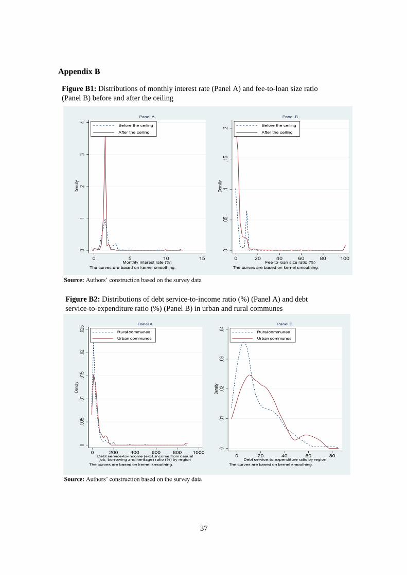
Tables 4 and 5 illustrate the monthly interest rate and loan assessment and processing fees

before and after the imposition of the interest rate ceiling in April 2017. For interest rate, the t-

test confirms the evidence of the decrease in the interest rates after the imposition for both loans

from all sources and loans from formal sources (i.e., MFIs). For loan assessment and processing

fees, while the difference of fee-to-loan size ratio before and after the ceiling imposition is not

statistically significant, the average fees per loan increased. The average monthly interest rate has

decreased from 1.82% to 1.60% for overall loan and from 1.82% to 1.57% for loan from formal

sources. The average interest rate after the ceiling imposition is very close to the legal ceiling rate,

which is 18% per year or around 1.5% monthly. Overall, average fee-to-loan size ratio is around

3% to 4% and has been almost the same before and after ceiling imposition, although average

fees per loan have increased from 28 USD to 44 USD for loans from overall sources and from 30

USD to 46 USD for loans from formal sources. The results indicating higher fees for loans from

formal sources should not be surprising, since loans from overall sources also include informal

sources that generally charge higher interest rates but may charge lower or no fees.

Generally, these results confirmed Hypothesis 1. That is, the imposition of the interest rate

ceiling has decreased the interest rates, thus reducing credit costs for borrowers. This might be

partially offset by the increase of the loan assessment and processing fees, although the offset

effect seems to be small.

15

𝑖

Table 4: Interest rates for loans before and after the ceiling imposition

Household category All sources Formal sources Before After Before After

S1 1.80 1.56 1.8 1.55 (Number of loans) (54) (241) (54) (232)

S2 1.77 1.75 1.77 1.45 (Number of loans) (60) (39) (60) (33)

S3 2.68 1.65 2.68 1.65 (Number of loans) (4) (94) (4) (92)

All categories 1.82 1.60 1.82 1.57 (Number of loans) (118) (374) (118) (357)

T-statistic of t-test for all

categories: One-tailed test 2.0758** 2.6290***

(H0: before=after)

Loans with zero interest rate are excluded from the calculation and estimation. Asterisks “***” and “**” indicate statistically significance at 1% and 5% significance levels, respectively.


Table 5: Loan assessment and processing fees before and after the ceiling imposition

Household

category

Average fees per loan in USD Fee-to-loan size ratio

All sources Formal sourcesa All sources Formal sourcesa

Asterisks “***” indicates statistically significance at 1% significance level. Source: Authors’ calculation and estimation based on the survey data.

5.1.2 Credit costs and their affecting factors

To compare the credit costs (i.e., interest rate and loan assessment and processing fees) before

and after the ceiling imposition in a more adequate manner, regression analyses on the

relationships between credit costs and their affecting factors are conducted. The regression

equation can be expressed as follows.

𝑦𝑖 = 𝑥′𝛽 + 𝑢𝑖, (1)

where 𝑦 is credit costs, 𝛽 = (𝛽0, 𝛽1, ⋯ , 𝛽𝑘)′ is a (𝑘 + 1) × 1 vector of regression coefficients,

𝑥 = (1, 𝑥1, ⋯ , 𝑥𝑘)′ is a (𝑘 + 1) × 1 vector of the explanatory variables, 𝑢 is the error term, and 𝑖

indicates the observation. For the specification of the estimation equations, the main factors

Before After Before After Before After Before After

S1 29.2 46.1 30.4 47.3 4.4 3.4 4.5 3.5 (Number of loans) (130) (444) (125) (425) (127) (442) (122) (425)

S2 27.6 28.7 28.8 32.0 1.7 3.9 1.8 4.4 (Number of loans) (140) (78) (134) (69) (137) (76) (131) (68)

S3 27.6 45.7 27.6 47.6 7.3 5.5 7.3 4.8 (Number of loans) (16) (200) (16) (187) (15) (200) (15) (187)

All categories 28.30 44.1 29.5 45.8 3.2 4.1 3.3 3.9 (Number of loans) (286) (722) (275) (681) (279) (718) (268) (680)

T-statistic of t-test

for all categories:

One-tailed test (H0: before=after)

-4.3194*** -4.3349*** -0.9626 -0.6589

16

𝑖 𝑖 𝑖 𝑖

affecting credit costs such as household characteristics, loan characteristics, market competition,

and common risk variables are taken into account. Household characteristics include household

IDPoor status, household income, average education years of household members, average age

of household members, number of household members (i.e., household size), household financial

literacy, and household head gender.6 Differences in these characteristics can result in different

household-specific risks and socio-economic conditions, which are taken into account by lenders

in financial transactions. Generally, a household with higher risk has higher credit costs. Loan

characteristics include loan size, loan maturity, loan collateral, loan source, and loan purpose. The

number of MFIs operating and non-performing loan rates at the commune level are used as

proxies for market competition and common risk variables, respectively. Dummy variables for

controlling the possible effects of different household categories and regional characteristics are

also incorporated into the estimation equation. Data used for the estimation are from our survey,

except for the number of MFIs operating and the non-performing loan rate, which are provided

by the CBC.

For the estimation method, the quantile regression (QR) method, developed by Koenker and

Bassett (1978), is applied. The quantile estimator of 𝛽 in Equation (1) is obtained from the

following optimization problem.

min 𝛽∈𝑅𝑘+1

[∑𝑖∈{𝑖: 𝑦𝑖≥𝑥′𝛽} ∅|𝑦𝑖 − 𝑥′𝛽| + ∑ 𝑖∈{𝑖: 𝑦𝑖<𝑥

′𝛽} (1 − ∅)|𝑦𝑖 − 𝑥′𝛽|], (2)

for the ∅𝑡ℎ (0<∅<1). The QR method allows us to examine the impact of explanatory variables at

the different quantiles of the distribution of the dependent variable. This method is more robust

than the conventional ordinary least squares (OLS) method if outliers in the data exist and when

the non-normal distribution pattern of the dependent variable is observed. From Figure B1 in

Appendix B, the distributions of monthly interest rate and fee-to-loan size ratio obviously have

non-normal patterns, and outliers may also exist in their data. This motivates our application of

the QR method. Tables 6 and 7 present the estimation results at the 25th, 50th, and 75th quantiles

25, 50, and 75, in which the monthly interest rate and fee-to-loan size ratio are used as dependent

variables, respectively.

6 Financial literacy of a household head or the spouse whom we interviewed is used as the proxy for

household financial literacy, since they are usually the main decision makers in their families. Financial

literacy is constructed by using survey questions related to households’ ability to calculate and understand

the economic variables such as interest rate and inflation calculations. The ratio of the correct answers in

all answers, which is between 0 and 1, is used as the measure of its level.

17

Table 6: Quantile regression results (dep. var.: monthly interest rate in %) Q.25th Before

(1-1)

Before

(1-2)

After

(1-3)

After

(1-4) Variable

IDPoor (Yes=1, No=0) -0.2649 -0.2617 -0.0087 -0.1266 (0.2004) (0.2029) (0.0248) (0.3549)

ln(income)a 0.0547 0.0546 -0.0034 -0.0011 (0.0605) (0.0609) (0.0094) (0.0096)

Ave. edu of hh member -0.0470* -0.0464* -0.0060 -0.0069 (0.0256) (0.0262) (0.0055) (0.0054)

ln(ave. age of hh member) -1.5765 -1.6656 0.9520* 0.9786* (4.2312) (4.2530) (0.5089) (0.5067)

Squared ln(ave. age of hh member) 0.2668 0.2795 -0.1453* -0.1492** (0.6107) (0.6123) (0.0755) (0.0751)

Household size -0.0357 -0.0359 -0.0031 -0.0035 (0.0515) (0.0533) (0.0074) (0.0071)

Financial literacy -0.2104 -0.2100 0.0322 0.0274 (0.3341) (0.3415) (0.0483) (0.0477)

Female hh head (Yes=1, No=0) 0.0937 0.0924 0.0034 0.0083 (0.1844) (0.1867) (0.0222) (0.0220)

ln(loan size) -0.0010 -0.0008 -0.0419*** -0.0420** (0.0602) (0.0602) (0.0156) (0.0162)

Loan's maturity -0.0047 -0.0047 -0.0030*** -0.0030*** (0.0035) (0.0035) (0.0011) (0.0011)

Land as collateral -0.0164 -0.0322 0.0084 0.0086 (0.3235) (0.3837) (0.0239) (0.0234)

Formal source (Yes=1, No=0)b - - -0.0558 -0.0565 - - (0.1954) (0.2311)

Productive and durable goods purpose -0.0270 -0.0275 -0.0150 -0.0165

(Yes=1, No=0) (0.1099) (0.1143) (0.0180) (0.0179)

Number of MFI loans per 100 hhs -0.4978* -0.5051 -0.0717* -0.0766* (2016 for before, 2018 for after) (0.2966) (0.3072) (0.0421) (0.0418)

Non-performing loan rate (%)c -0.0030 -0.0025 -0.0026 -0.0044

(2016 for before, 2018 for after) (0.0315) (0.0342) (0.0118) (0.0119) S1 dummy (S1=1, Other=0) -0.2480 0.0318 0.0164 0.0150

(0.9400) (1.0409) (0.0271) (0.0257)

S2 dummy (S2=1, Other=0) -0.0448 0.2385 -0.0021 -0.0051 (0.9421) (1.0431) (0.0433) (0.0417)

Urban commune dummy (Yes=1, No=0) 0.3331* 0.3302* -0.0087 -0.0002 (0.1863) (0.1882) (0.0403) (0.0422)

IDPoor*Formal source - 0.1233 - (0.3554)

IDPoor*Urban commune dummy -0.0173 -0.0618 (0.5581) (0.0682)

Constant 4.3778 4.2703 0.4153 0.3711 (7.2376) (7.3017) (0.8512) (0.8527)

Number of observations 110 110 368 368

Pseudo-R2 0.133 0.133 0.178 0.180 a Income from casual job, borrowing and heritage are excluded. b Coefficients of “formal source” in columns 1-1 and 1-2 cannot be estimated, due to too few data for number of loans from informal sources. c Non-performing loan refer to loan whose payment was more than 30-day overdue. Results are based on 10,000 bootstrapping repetitions. The number in parentheses is the standard error.

Asterisk “***”, “**” and “*” indicate the statistical significance at 1%, 5% and 10% significance levels, respectively.

18

Table 6 (cont.): Quantile regression results (dep. var.: monthly interest rate in %)

Q.50th Before Before After After

Variable (2-1) (2-2) (2-3) (2-4)

IDPoor (Yes=1, No=0) -0.1732 -0.1676 -0.0099 -0.5467 (0.2528) (0.2682) (0.0152) (0.3821)

ln(income)a -0.0002 0.0003 -0.0012 -0.0006 (0.0699) (0.0706) (0.0089) (0.0092)

Ave. edu of hh member -0.0203 -0.0260 -0.0036 -0.0036 (0.0330) (0.0337) (0.0038) (0.0038)

ln(ave. age of hh member) -2.8859 -1.4232 0.4277 0.3542 (4.6500) (4.7286) (0.4285) (0.4427)

Squared ln(ave. age of hh member) 0.4470 0.2231 -0.0653 -0.0539 (0.6792) (0.6890) (0.0638) (0.0659)

Household size -0.0411 -0.0423 -0.0037 -0.0039 (0.0729) (0.0746) (0.0052) (0.0053)

Financial literacy -0.0461 0.0372 0.0234 0.0198 (0.4388) (0.4455) (0.0361) (0.0365)


ln(loan size) -0.0543 -0.0758 -0.0439** -0.0438** (0.0966) (0.0974) (0.0172) (0.0176)

Loan's maturity -0.0042 -0.0031 -0.0018* -0.0018* (0.0051) (0.0051) (0.0010) (0.0011)

Land as collateral -0.0337 -0.0627 0.0385* 0.0377* (0.3988) (0.4435) (0.0207) (0.0210)

Formal source (Yes=1, No=0)b - - -0.3821** -0.3825 - - (0.1779) (0.2422)

Productive and durable goods purpose -0.0153 0.0051 -0.0118 -0.0112

(Yes=1, No=0) (0.1413) (0.1447) (0.0167) (0.0170)

Number of MFI loans per 100 hhs -0.1596 -0.1601 -0.0546* -0.0575* (2016 for before, 2018 for after) (0.3347) (0.3495) (0.0309) (0.0325)

Non-performing loan rate (%)c -0.0073 -0.0045 -0.0050 -0.0052

(2016 for before, 2018 for after) (0.0400) (0.0481) (0.0068) (0.0070)

S1 dummy (S1=1, Other=0) -1.2736 -1.3018 -0.0016 -0.0029 (1.1944) (1.2973) (0.0175) (0.0179)

S2 dummy (S2=1, Other=0) -1.1450 -1.1838 -0.0323 -0.0320 (1.2015) (1.2988) (0.0357) (0.0361)

Urban commune dummy (Yes=1, No=0) 0.0644 0.1492 0.0070 0.0085 (0.2442) (0.2541) (0.0277) (0.0397)



Constant 8.3559 6.1707 1.5999** 1.7185** (7.7818) (8.0164) (0.7095) (0.7519)


Pseudo-R2 0.085 0.086 0.045 0.045 a Income from casual job, borrowing and heritage are excluded. b Coefficients of “formal source” in columns 2-1 and 2-2 cannot be estimated, due to too few data for number of loans from informal sources. c Non-performing loan refer to loan whose payment was more than 30 days overdue.

Results are based on 10,000 bootstrapping repetitions. The number in parentheses is the standard error. Asterisk “***”, “**” and “*” indicate the statistical significance at 1%, 5% and 10% significance levels, respectively.

19

Table 6 (cont.): Quantile regression results (dep. var.: monthly interest rate in %) Q.75th Before

(3-1)

Before

(3-2)

After

(3-3)

After

(3-4) Variable

IDPoor (Yes=1, No=0) -0.2315 0.0406 -0.0000 -0.6000 (0.4068) (0.4706) (0.0319) (1.2072)

ln(income)a 0.0247 -0.0513 0.0000 -0.0000 (0.1000) (0.1028) (0.0162) (0.0165)

Ave. edu of hh member -0.0077 -0.0157 0.0000 -0.0000 (0.0566) (0.0572) (0.0074) (0.0075)

ln(ave. age of hh member) 1.2248 3.1363 -0.0000 0.0000 (8.6932) (8.4312) (0.8471) (0.8347)

Squared ln(ave. age of hh member) -0.1402 -0.4198 0.0000 -0.0000 (1.2419) (1.2015) (0.1255) (0.1236)

Household size 0.0235 -0.0546 0.0000 0.0000 (0.1250) (0.1261) (0.0090) (0.0090)

Financial literacy 0.3924 0.1735 0.0000 -0.0000 (0.7231) (0.7457) (0.0596) (0.0613)

Female hh head (Yes=1, No=0) 0.6430* 0.4105 -0.0000 -0.0000 (0.3794) (0.3796) (0.0404) (0.0409)

ln(loan size) -0.2874 -0.2410 0.0000 0.0000 (0.1753) (0.1719) (0.0398) (0.0400)

Loan's maturity 0.0010 -0.0011 0.0000 0.0000 (0.0107) (0.0107) (0.0016) (0.0017)

Land as collateral 0.1413 -0.3412 -0.0000 -0.0000 (0.5441) (0.5808) (0.0728) (0.0702)

Formal source (Yes=1, No=0)b - - -1.0000 -1.0000 - - (0.8687) (1.1829)

Productive and durable goods purpose 0.1947 0.0556 0.0000 0.0000

(Yes=1, No=0) (0.3212) (0.3276) (0.0248) (0.0255)

Number of MFI loans per 100 hhs 0.0990 0.0979 -0.0000 -0.0000 (2016 for before, 2018 for after) (0.5837) (0.6051) (0.0462) (0.0502)

Non-performing loan rate (%)c -0.0216 0.0427 0.0000 0.0000

(2016 for before, 2018 for after) (0.0645) (0.0777) (0.0192) (0.0211) S1 dummy (S1=1, Other=0) -0.1483 -1.4866 0.0000 0.0000

(1.3308) (1.3971) (0.0389) (0.0400)

S2 dummy (S2=1, Other=0) -0.2493 -1.5993 -0.0000 0.0000 (1.3241) (1.3920) (0.0707) (0.0683)

Urban commune dummy (Yes=1, No=0) -0.1753 -0.0108 0.0000 -0.0000 (0.4651) (0.4987) (0.0690) (0.1163)



Constant 1.2943 0.3610 2.5000 2.5000 (14.9810) (14.6452) (1.5231) (1.7358)


Pseudo-R2 0.175 0.191 0.045 0.049 a Income from casual job, borrowing and heritage are excluded. b Coefficients of “formal source” in columns 3-1 and 3-2 cannot be estimated, due to too few data for number of loans from informal sources. c Non-performing loan refer to loan whose payment was more than 30 days overdue. Results are based on 10,000 bootstrapping repetitions. The number in parentheses is the standard error.


20

Table 7: Quantile regression results (dep. var.: fee-to-loan size ratio, %) Q.25th Before

(1-1)

Before

(1-2)

After

(1-3)

After

(1-4) Variable

IDPoor (Yes=1, No=0) -0.0057 -0.0186 0.0209 0.2866 (0.1224) (0.3239) (0.1259) (4.5776)

ln(income)a -0.0048 -0.0051 0.0285 0.0116 (0.0477) (0.0489) (0.0391) (0.0425)

Ave. edu. of hh member -0.0158 -0.0170 0.0133 0.0072 (0.0261) (0.0268) (0.0176) (0.0174)

ln(ave. age of hh member) 3.3775 3.0799 -3.4911 -2.8216 (3.3880) (3.4262) (2.5391) (2.4005)

Squared ln(ave. age of hh member) -0.5640 -0.5215 0.4737 0.3741 (0.4884) (0.4935) (0.3623) (0.3423)

Household size -0.0694 -0.0652 -0.0122 -0.0119 (0.0445) (0.0459) (0.0292) (0.0279)

Financial literacy 0.3658* 0.3589 -0.0646 -0.1178 (0.2188) (0.2302) (0.1928) (0.1883)

Female hh head (Yes=1, No=0) 0.0491 0.0467 -0.0540 -0.0680 (0.1104) (0.1150) (0.0954) (0.0903)

ln(loan size) -0.1392* -0.1456* -0.0552 -0.0578 (0.0716) (0.0751) (0.0637) (0.0691)

Loan's maturity -0.0031 -0.0026 -0.0008 -0.0005 (0.0029) (0.0030) (0.0023) (0.0022)

Land as collateral 0.2327 0.2440 0.1124 0.0906 (0.3351) (0.3340) (0.2003) (0.1827)

Formal source (Yes=1, No=0) 0.6615* 0.6569 0.2289 0.3712 (0.3730) (0.4101) (0.2489) (0.2804)

Productive and durable goods purpose -0.0786 -0.0781 0.1239 0.1420 (Yes=1, No=0) (0.0981) (0.0983) (0.0886) (0.0875)

Number of MFI loans per 100 hhs -0.1449 -0.1112 0.0332 0.0981 (2016 for before, 2018 for after) (0.1991) (0.2126) (0.1092) (0.1120)

Non-performing loan rate (%)b -0.0027 -0.0093 -0.0084 -0.0111


S1 dummy (S1=1, Other=0) 0.2399 0.2246 0.1094 0.1177 (0.2660) (0.2736) (0.0961) (0.0956)

S2 dummy (S2=1, Other=0) 0.0842 0.0772 -0.0155 0.0099 (0.2563) (0.2625) (0.1170) (0.1237)

Urban commune dummy (Yes=1, No=0) -0.4164*** -0.4100** 0.0162 -0.0242 (0.1534) (0.1760) (0.1089) (0.1110)

IDPoor*Formal source -0.0591 -0.3648 (0.3634) (4.5727)

IDPoor*Urban commune dummy 0.1539 0.0388 (0.3948) (0.3751)

Constant -3.8122 -3.2783 6.3829 5.2629 (5.7390) (5.8250) (4.4157) (4.1991)


Pseudo-R2 0.038 0.038 0.008 0.008 a Income from casual job, borrowing and heritage are excluded. b Non-performing loan refer to loan whose payment was more than 30 days overdue. Results are based on 10,000 bootstrapping repetitions. The number in parentheses is the standard error.


21

Table 7 (cont.): Quantile regression results (dep. var.: fee-to-loan size ratio, %) Q.50th Before

(2-1)

Before

(2-2)

After

(2-3)

After

(2-4) Variable

IDPoor (Yes=1, No=0) -0.0358 0.0082 0.2068 1.2531 (0.1280) (0.4478) (0.1858) (12.8876)

ln(income)a 0.0588 0.0559 0.0209 0.0234 (0.0669) (0.0640) (0.0717) (0.0707)

Ave. edu. of hh member -0.0297 -0.0309 -0.0134 -0.0013 (0.0246) (0.0248) (0.0364) (0.0356)

ln(ave. age of hh member) -2.7878 -2.5170 -4.9823 -5.4504 (4.8695) (4.9843) (4.8533) (4.7361)

Squared ln(ave. age of hh member) 0.3341 0.2952 0.6610 0.7289 (0.6874) (0.7040) (0.6889) (0.6728)

Household size -0.0385 -0.0347 -0.0660 -0.0536 (0.0459) (0.0458) (0.0430) (0.0422)

Financial literacy -0.0092 -0.0092 -0.1712 -0.1697 (0.2814) (0.2831) (0.3190) (0.3178)

Female hh head (Yes=1, No=0) 0.1031 0.0986 -0.0937 -0.1178 (0.1195) (0.1219) (0.1527) (0.1497)

ln(loan size) -0.3494** -0.3558** -0.5610*** -0.5736*** (0.1518) (0.1486) (0.1086) (0.1099)

Loan's maturity 0.0027 0.0034 0.0013 0.0022 (0.0062) (0.0062) (0.0037) (0.0037)

Land as collateral -0.2177 -0.1623 -0.1964 -0.3239 (0.8784) (0.8503) (0.3632) (0.3460)

Formal source (Yes=1, No=0) 1.6720* 1.6200* 2.0764*** 2.6227*** (0.9429) (0.9591) (0.6005) (0.5535)

Productive and durable goods purpose -0.1226 -0.1167 0.1687 0.1911 (Yes=1, No=0) (0.1178) (0.1172) (0.1450) (0.1413)

Number of MFI loans per 100 hhs -0.2084 -0.2090 0.1072 0.1249 (2016 for before, 2018 for after) (0.2621) (0.2613) (0.1723) (0.1673)

Non-performing loan rate (%)b 0.0223 0.0244 0.0517 0.0323


S1 dummy (S1=1, Other=0) 0.1232 0.0760 0.0780 0.0731 (1.9744) (1.4059) (0.1593) (0.1584)

S2 dummy (S2=1, Other=0) 0.0539 -0.0248 -0.4863** -0.3720 (1.9717) (1.4007) (0.2284) (0.2275)

Urban commune dummy (Yes=1, No=0) -0.1112 -0.0814 -0.0706 -0.2094 (0.1940) (0.2261) (0.1696) (0.1724)

IDPoor*Formal source -0.0272 -1.2739 (0.4825) (12.8916)

IDPoor*Urban commune dummy -0.0537 0.2911 (0.4651) (0.4774)

Constant 7.7225 7.3378 13.0899 13.4427* (8.8567) (8.9103) (8.2410) (8.1009)




22

Table 7 (cont.): Quantile regression results (dep. var.: fee-to-loan size ratio, %) Q.75th Before

(3-1)

Before

(3-2)

After

(3-3)

After

(3-4) Variable

IDPoor (Yes=1, No=0) -0.5536* -0.5563 -0.1824 7.3588 (0.3346) (1.6355) (0.4056) (39.3057)

ln(income)a 0.0410 0.0220 0.1382 0.1803 (0.1478) (0.1496) (0.1346) (0.1341)

Ave. edu. of hh member -0.0116 -0.0102 -0.0352 -0.0472 (0.0681) (0.0725) (0.0706) (0.0684)

ln(ave. age of hh member) -2.2803 -0.1731 -10.5367 -7.4577 (13.9287) (14.6582) (9.1511) (8.8049)

Squared ln(ave. age of hh member) 0.2191 -0.0971 1.4776 1.0472 (1.9587) (2.0622) (1.3030) (1.2538)

Household size -0.0485 -0.0784 -0.0489 -0.0455 (0.1476) (0.1545) (0.0931) (0.0827)

Financial literacy 0.7327 0.7805 0.0409 -0.0595 (0.6841) (0.7134) (0.6583) (0.6109)

Female hh head (Yes=1, No=0) 0.1584 0.2495 -0.5281* -0.5054* (0.4208) (0.4343) (0.2941) (0.2699)

ln(loan size) -1.1027** -1.0043** -1.7196*** -1.6246*** (0.4721) (0.4799) (0.2183) (0.2033)

Loan's maturity 0.0136 0.0126 0.0115* 0.0108* (0.0149) (0.0154) (0.0064) (0.0063)

Land as collateral -5.9887** -6.0473** -1.0890 -1.2469* (2.7221) (2.5724) (0.7551) (0.7568)

Formal source (Yes=1, No=0) 8.6604*** 8.4685*** 1.6397 3.8678** (2.6065) (2.6194) (2.2119) (1.5352)

Productive and durable goods purpose -0.2065 -0.3137 0.2006 0.2635

(Yes=1, No=0) (0.2709) (0.2771) (0.2723) (0.2634)

Number of MFI loans per 100 hhs 0.0164 -0.1663 0.5592* 0.5275* (2016 for before, 2018 for after) (0.7709) (0.7906) (0.3028) (0.2961)

Non-performing loan rate (%)b 0.0676 0.0787 0.1267 0.0955


S1 dummy (S1=1, Other=0) 0.4407 0.5970 0.1883 0.1461 (13.4458) (12.7971) (0.3302) (0.3152)

S2 dummy (S2=1, Other=0) 0.3900 0.4721 -0.7683** -0.6640* (13.4471) (12.8004) (0.3856) (0.3778)

Urban commune dummy (Yes=1, No=0) -0.0541 0.1407 -0.0275 -0.3124 (0.6226) (0.6845) (0.4357) (0.3955)

IDPoor*Formal source 0.0996 -7.8543 (1.6862) (39.3159)


Constant 11.8895 8.0885 33.2348** 24.8458* (28.9981) (29.8975) (16.0104) (15.0383)



Asterisk “***”, “**” and “*” indicate the statistical significance at 1%, 5% and 10% significance level, respectively.

23

Using the fitted values of the monthly interest rate calculated from the 50th quantile results in

Table 6, after the ceiling imposition, the average monthly interest rate decreased from 1.69% to

1.46%, which is well below the ceiling rate.7 If only loans from formal sources are considered, it

decreased to 1.44%. These results reflect the fact that the ceiling rate is being effectively enforced,

although only about 13% of our 1,000 survey households answered that they are aware of the

interest rate ceiling policy.8 Table 6 also indicates that, after the ceiling imposition, the lower

interest rate seems to be significantly correlated with a higher number of MFIs operating, which

is a proxy for microfinance market competition, based on the results from the 25th and 50th

quantiles. This finding implies that a higher competition among MFIs can result in a lower interest

rate. Moreover, the table shows that the lower interest rate seems to be associated with a larger

loan size and longer loan maturity. As for fee-to-loan size ratio, after the ceiling imposition, it has

increased from 0.90% to 1.45%, using its fitted values calculated from quantile 50th results in

Table 7.9 The table shows that, overall, the higher fee-to-loan size ratio seems to be significantly

associated with the larger loan size. It also has a significantly positive correlation with loans from

formal sources. This positive correlation result should not be surprising. Formal lenders generally

need to follow various formal procedures during the loan assessment and processing that incurs

fees. Although informal lenders might not apply such procedures when providing loans, they

generally charge higher interest rates.

Our findings confirmed Hypothesis 1, as also evidenced by the basic statistics results. That

is, while the ceiling imposition has resulted in the decrease of the interest rate for borrowers, this

could be partially offset by the increase in loan assessment and processing fees. Overall, these

findings are consistent with those of World Bank (2019) from the analysis based on data and

information from MFIs.

5.2 Interest rate ceiling, loan size, and loan maturity

Table 8 illustrates the average loan size and loan maturity before and after the imposition of

the interest rate ceiling. The table shows that there is no statistically significant evidence of the

change of the overall average loan size and loan maturity after the ceiling imposition. Overall, the

average loan size is around 4,000 USD, and the average loan maturity is around 30 months. Figure

7 Estimated coefficients in columns 2-1 and 2-3 in Table 6 are used to calculate the fitted values of the

interest rate before and after the ceiling imposition, respectively. 8 From our survey, three fourths of those who are aware of the existence of the interest rate ceiling answered

that they knew about it from credit officers of MFIs. 9 Fitted values of the fee-to-loan size ratio before and after the ceiling imposition are calculated by using

estimated coefficients in columns 2-1 and 2-3 in Table 7, respectively.

24

3 illustrates the distribution of the loan size before and after the ceiling by loan source. From the

figure, the obvious difference of loan size cannot be observed as well. However, Table 9 illustrates

the statistical evidence on the increase of the average loan size at a relatively small loan level after

the ceiling imposition, in the case of loans from formal sources.

Overall, our finding could not strongly confirm Hypothesis 2, since the difference in the

average loan maturity before and after the ceiling imposition is not statistically significant.

However, the evidence on the increase of the average loan size for a relatively small loan may

provide some implications on debt burden among relatively small borrowers, as discussed later.

Table 8: Loan size and loan maturity before and after the ceiling imposition

Household

category

Average loan size (USD)

All sources Formal sources

Average loan maturity (months)

All sources Formal sources Before After Before After Before After Before After

S1 3,621 4,665 3,746 4,970 30.0 29.8 30.9 30.5 (Number of loans) (127) (446) (122) (429) (145) (448) (140) (429)

S2 4,020 3,721 4,181 4,046 31.7 26.5 33.1 28.8 (Number of loans) (138) (78) (132) (68) (144) (77) (138) (68)

S3 3,578 3,921 3,578 4,141 28.6 29.4 28.6 31.2 (Number of loans) (15) (201) (15) (187) (16) (200) (16) (186)

All categories 3,816 4,357 3,950 4,539 30.7 29.3 31.8 30.5 (Number of loans) (280) (725) (269) (684) (305) (725) (294) (683)

T-statistic of t-test for all

categories: One-tailed test -1.3657 -1.4306 0.9414 0.8259 (H0: before=after)


Table 9: Loan size (USD) by range before and after the ceiling imposition, formal sources

Loan size Average T-statistic of t-test

Before After (H0: before=after)

less than 1,000 loan size 425 495 -2.3749*** (Number of loans) (67) (207)

1,000 ≤ loan size < 2,000 1,243 1,254 -0.1987 (Number of loans) (28) (92)

2,000 ≤ loan size < 3,000 2,114 2,209 -1.9631** (Number of loans) (44) (71)

3,000 ≤ loan size < 4,000 3,052 3,086 -0.8529 (Number of loans) (31) (52)

4,000 ≤ loan size < 5,000 4,156 4,086 1.0831 (Number of loans) (16) (28)

5,000 ≤ loan size < 6,000 5,023 5,037 -0.5506

(Number of loans) (30) (54)

loan size ≥ 6,000 11,217 12,127 -0.8161 (Number of loans) (53) (180)

Asterisks “***” and “**” indicate statistical significance at 1% and 5% significance levels, respectively. Source: Authors’ calculation and estimation based on the survey data

25

Figure 3: Distributions of loan size for all sources (Panel A) and formal sources (Panel B)

before and after the ceiling, formal sources only


5.3 Interest rate ceiling and informal credit

Table 10 presents the percentage of loans from informal sources before and after the ceiling

imposition. The table indicates that loans from informal sources significantly increased by a few

percentage points. Overall, this result confirmed Hypothesis 3-1 regarding the increase in

informal credit, if informal lenders are prevailing in the market. This could reflect the possibility

of credit rationing by formal lenders, as a result of the ceiling imposition, although more

sophisticated study might be needed to assess this consequence.

From our survey, among 595 households who provided answers, 56 households answered

that they had experience being rejected for a loan by formal lenders after the ceiling imposition.

Table 11 illustrates the reasons for the households’ experience with loan rejection in Panel A and

the households’ coping methods in Panel B. From the table, lack of collateral and too-low income

or being judged as having too low ability for loan repayment by the lenders seem to be the main

reasons for being rejected for loans. Nearly half of the households with experience being rejected

for a loan turned to borrow from informal lenders such as friends and money lenders.

26

Table 10: Percentage of loans from informal sources before and after the ceiling imposition

Household

category

% of loans from informal sourcesa

Before After

S1 3.4 4.2 (Number of loans) (146) (448)

S2 4.2 11.5 (Number of loans) (144) (78)

S3 0.0 7.0 (Number of loans) (16) (201)

All categories 3.6 5.8 (Number of loans) (306) (727)

T-statistic of t-test for all categories: One-tailed test (H0: before=after)

-1.4517*

a Loans from village banks are categorized as loans from formal sources. Asterisks “*” indicates statistical significance at 10% significance level. Source: Authors' calculation and estimation based on the survey data.

Table11: Reasons of being rejected for loan and households’ coping methods Panel A: Reasons % of householdsa

Too small borrowing amountb 7.1 (number of households) (4)

Lack of collateral 30.4 (number of households) (17)

Having too low income or being judged

having too low ability in loan repayment 46.4

(number of households) (26)

Other reasons (late repayment of previous loan, etc.) 7.1 (number of households) (4)

Unaware of reason 19.6 (number of households) (11)

Panel B: Coping methods % of householdsa

Reducing necessary consumption 1.8 (number of households) (1)

Selling livestock (cattle, buffalo, etc.) 5.4 (number of households) (3)

Selling lands 5.4 (number of households) (3)

Selling durable goods (agricultural tools, motorbike, etc.) 5.4 (number of households) (3)

Borrowing from informal sources (relatives, money lenders, etc.) 44.6 (number of households) (25)

Other solution 1.8 (number of households) (1)

Do nothing 42.9 (number of households) (24)

Total number of households

experiencing being rejected for loan 56

a Households can be rejected for loan by more than one reasons and they can also have more than one coping methods. b Specific borrowing amounts were 200 USD, 250 USD, 750 USD and 1,000 USD. Source: Authors’ calculation and estimation, based on the survey data.

27

𝑖

5.4 Household characteristics and experience being rejected for loans

To examine the factors affecting the experience being rejected for a loan in a more adequate

manner, logistic and probit regression analyses are applied by focusing on household

characteristics. The regression equation can be expressed as follows.

𝑃𝑟(𝑟𝑖 = 1|𝑑𝑖) = 𝑑′𝛾 + 𝑣𝑖, (3)

where 𝑟 takes the value of 1 for a household having experience being rejected for a loan and 0

otherwise, 𝛾 = (𝛾0, 𝛾1, ⋯ , 𝛾𝑙)′ is a (𝑙 + 1) × 1 vector of regression coefficients, 𝑑 =

(1, 𝑑1, ⋯ , 𝑑𝑙)′ is a (𝑙 + 1) × 1 vector of the explanatory variables, 𝑣 is the error term, and 𝑖

indicates the observation. Explanatory variables include main household characteristic variables

such as household IDPoor status, household income, average education years of household

members, average age of household members, number of household members (i.e., household

size), household financial literacy, and head of household gender. Differences in these

characteristics can result in a different probability of being rejected for loan lenders. Dummy

variables addressing the possible effects of different household categories and regional

characteristics are also incorporated into the estimation equation. Data used for the estimation are

from our survey.

The estimation results are provided in Table 12. From the table, overall, the coefficients of

household income, average age of household members, and its squares are statistically significant.

Higher probability of being rejected for a loan is significantly associated with lower household

income. Given that the sign of squared average age of household members is negative, households

with too young age members and too old age members tend to face higher probability of being

rejected for a loan. In general, households with too young age members or too old age members

have a higher age dependency ratio. This can negatively reflect their ability for loan repayment

as judged by lenders. Evidence from Table 12 is consistent with the basic statistics results in Table

11. That is, low income or being judged as having too low ability for loan repayment by lenders

seem to be the main reasons for being rejected for loans.

28

Table 12: Logistic and probit regression results (dep. var.: experience of loan rejection, yes=1, no=0)

Variable

Logistic

Logistic

Probit

Probit (1) (2) (3) (4)

IDPoor (Yes=1, No=0) 0.3423 0.3410 0.1824 0.1794 (0.3199) (0.3183) (0.1646) (0.1633)

ln(income)a -0.2289 -0.2308* -0.1243* -0.1253* (0.1393) (0.1392) (0.0721) (0.0722)

Ave. edu. of hh member 0.0317 0.0259 0.0140 0.0111 (0.0720) (0.0721) (0.0359) (0.0364)

ln(ave. age of hh member) 17.0185* 17.0372* 9.0353* 9.0444* (9.1795) (9.2047) (4.6480) (4.6628)

Squared ln(ave. age of hh member) -2.6677** -2.6692* -1.4090** -1.4096** (1.3604) (1.3639) (0.6853) (0.6874)

Household size 0.1182 0.1178 0.0616 0.0617 (0.0877) (0.0884) (0.0457) (0.0459)

Financial literacy 0.5887 0.6034 0.3069 0.3141 (0.7125) (0.7113) (0.3615) (0.3618)


S1 dummy (S1=1, Other=0) 0.1230 0.1270 0.0702 0.0710 (0.3394) (0.3415) (0.1694) (0.1698)

S2 dummy (S2=1, Other=0) 0.7065 0.7149 0.3939 0.3980 (0.5115) (0.5132) (0.2637) (0.2643)

Urban commune dummy

(Yes=1, No=0)

0.1157

0.0563

(0.3331) (0.1707)

Constant -28.9454* -28.9895* -15.5272** -15.5472** (15.2405) (15.2831) (7.7434) (7.7690)

Number of observations 581 581 581 581 Log pseudolikelihood -172.637 -172.5783 -172.403 -172.351

Pseudo-R2 0.051 0.052 0.053 0.053 a Income from casual job, borrowing and heritage are excluded. The number in parentheses is the robust standard error. Asterisk “**” and “*” indicate the statistical significance at 5% and 10% significance levels, respectively.

5.5 Household debt burden

As discussed above, the rationale underlying the imposition of the interest rate ceiling in the

microfinance sector is the need to protect borrowers from being charged too high interest rate and

the need to adjust the short-sighted and time-inconsistent behavior of borrowers. This can be a

result of the concern regarding the debt burden among borrowers. In this study, although the

sophisticated examination of the impacts of the ceiling imposition on debt burden cannot be

conducted due to data and information limitations, an illustration of debt burden and an analysis

of its affecting factors are provided, including the test of Hypothesis 3-2 regarding the role of

financial literacy in reducing debt burden.

29

5.5.1 Basic statistics

Table 13 illustrates the basic statistics of household debt service-to-income ratio and the

debt service-to-expenditure ratio. These statistics are based on data from the survey on households

reporting to have debt service expenditures. The table shows that, overall, the debt service ratio

of urban households is higher than that of rural households. This result may reflect the fact that

urban households engage more actively in financial transactions, and their borrowing amount is

generally larger. Moreover, the debt service-to-income ratio seems to be more volatile and more

prone to suffer from the existence of outliers than the debt service-to-expenditure ratio. This

should not be surprising, given the more volatile characteristics of household incomes compared

to household expenditures in general.

Figure 4 presents the cumulative distributions of debt service-to-income ratio (Panel A) and

the debt service-to-expenditure ratio (Panel B) in urban and rural communes. The vertical lines in

both panels indicates 50% of the of debt service ratio level. Overall, the percentages of borrower

households having a debt service ratio of more than 50% are about 18% for debt service-to-

income ratio and about 5% for debt service-to-expenditure ratio. These percentages are somewhat

higher among households in urban communes.

Table 13: Household debt service ratio

Debt service-to-income ratio (%)a Debt service-to-expenditure ratio (%)

Basic statistics Urban

communes

Rural

communes

All

communes

Urban

communes

Rural

communes

All

communes Average 49.0 32.2 35.9 20.6 16.2 17.3

Median 24.0 15.2 17.5 18.0 10.4 12.1

Minimum 0.1 0.1 0.1 0.2 0.1 0.1

Maximum 888.9 500.0 888.9 62.6 80.5 80.5

Standard deviation 113.5 53.0 71.0 16.9 15.9 16.2

Number of households 63 223 286 68 228 296

T-statistic of t-test: One-

tailed test

-1.6677**

-1.9678**

(H0: Ave. urban=Ave. rural)

a Income from casual job, borrowing and heritage are excluded.

Asterisks “**” indicate statistically significance at 5% significance level. Source: Authors’ calculation and estimation, based on the survey data.

30

𝑖

Figure 4: Cumulative distributions of debt service-to-income ratio (Panel A) and debt service-

to-expenditure ratio (Panel B) in urban and rural communes


5.5.2 Household debt burden and its affecting factors

To examine factors affecting debt burden, regression analyses on the relationships between

household debt service ratio and its affecting factors are conducted. The regression equation can

be expressed as follows.

𝑧𝑖 = ℎ′𝜃 + 𝜇𝑖, (4)

where 𝑧 is household debt service ratio, 𝜃 = (𝜃0, 𝜃1, ⋯ , 𝜃𝑚)′ is a (𝑚 + 1) × 1 vector of

regression coefficients, ℎ = (1, ℎ1, ⋯ , ℎ𝑚)′ is a (𝑚 + 1) × 1 vector of the explanatory variables,

𝜇 is the error term, and 𝑖 indicates the observation. Two debt service ratios are considered for the

estimation: debt service-to-income ratio and debt service-to-expenditure ratio. The specification

of the estimation equations takes into account household characteristics, loan characteristics,

market competition, and common risk variables. Similar to the specification in the case of credit

cost analyses in Equation (1), household characteristics include household IDPoor status,

household income, average education years of household members, average age of household

members, number of household members (i.e., household size), household financial literacy, and

household head gender. Loan characteristics include loan size and the percentage of informal-

source loans possessed by borrower households in the total loan numbers. As proxy variables for

31

the market competition and common risk variables, the number of MFIs operating and non-

performing loan rate at the commune level is used. To control for the possible effects of different

household categories and regional characteristics, household category, and regional dummy

variables are also included in the estimation equation. Except for the number of MFIs operating

and non-performing loan rate which are provided by the CBC, all data are from our survey. For

the estimation method, like the cause of credit cost analyses, we apply the QR method that allows

us to examine the factors affecting the debt service ratio at different quantiles of its distribution.

Figure B2 in Appendix B also motivates our application of the QR method. From the figure, the

distributions of dependent variables, debt service-to-income ratio, (Panel A) and debt service-to-

expenditure ratio (Panel B) obviously have non-normal patterns, and outliers may also exist in

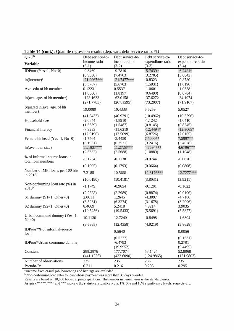
their data, especially for the former. Table 14 presents the estimation results at the 25th, 50th, and

75th quantiles of the dependent variable.

Table 14 show that higher debt service ratio is significantly associated with larger loan size.

A 10% increase in loan size is associated with an increase of about 0.3% to 0.5% in debt service-

to-expenditure ratio. These results may have some implications. Since the increase in the loan

size at the relatively small loan level is observed after the ceiling imposition, the positive

correlation between loan size and debt service ratio might somewhat imply a possibility of the

increase in debt burden among the relatively small borrower households. Furthermore,

households with female household heads seem to be positively associated with higher debt

service-to-expenditure ratios of about 2% to 8%. The higher debt service ratio of households with

female household heads reflects the fact that their income and expenditures are relatively low,

compared to households with male household heads. Overall, our estimation results also indicate

that a lower debt service ratio is significantly associated with higher financial literacy level. A 0.1

increase in financial literacy is associated with about 1% decrease in debt service-to-expenditure

ratio at the 50th and 75th quantiles of the estimation.10 This decreasing effect seems to be larger at

a higher debt service-to-expenditure ratio. The evidence on the important role of financial literacy

in reducing debt burden is in line with Live (2013), which indicated that a higher financial literacy

could reduce a borrower’s inclination for an over-indebtedness. Our estimation results confirmed

Hypothesis 3-2. The significant results of the positive correlation between the debt service ratio

and the number of MFIs operating should not be surprising, since a higher number of operating

MFIs reflects higher household credit access, resulting in higher household debt service ratio.

10 As explained above, by construction, financial literacy level is between 0 and 1. A higher value reflects

a higher literacy level. Average financial literacy of our surveyed households is about 0.3 in both rural and

urban communes.

32

Table 14: Quantile regression results (dep. var.: debt service ratio, %)

Q.25th Debt service-to- Debt service-to- Debt service-to- Debt service-to-

Variable income ratio income ratio expenditure ratio expenditure ratio

% of informal-source loans in

total loan numbers

Number of MFI loans per 100

hhs in 2018

Non-performing loan rate (%) in

0.0164 -0.0287 0.0459 0.0379

(0.0567) (0.0729) (0.0294) (0.0424)

8.1461*** 8.6068** 7.5682*** 7.4940***

(3.0459) (3.4639) (2.1672) (2.3098)

0.7633 0.8263 0.8288* 0.8787**

a Income from casual job, borrowing and heritage are excluded. b Non-performing loan refer to loan whose payment was more than 30 days overdue. Results are based on 10,000 bootstrapping repetitions. The number in parentheses is the standard error. Asterisk “***”, “**” and “*” indicate the statistical significance at 1%, 5% and 10% significance levels, respectively.

(1-1) (1-2) (1-3) (1-4)

IDPoor (Yes=1, No=0) -0.3798 -0.3044 -0.2987 -0.0850 (2.6438) (2.9679) (1.5869) (1.7477)

ln(income)a -6.6663*** -6.6760*** -0.8482 -1.0166 (1.8455) (1.8618) (0.6246) (0.6685)


ln(ave. age. of hh member) -21.4542 -24.3749 -70.2111* -71.8917* (69.8320) (71.1691) (41.8931) (43.3954)

Squared ln(ave. age. of hh member)

3.2154 3.5693 10.8910* 11.2172*

(10.1976) (10.3835) (6.1647) (6.3877)

Household size -0.1019 -0.1605 -0.2604 -0.2955 (0.5852) (0.6012) (0.2738) (0.2940)

Financial literacy -0.8404 -0.6135 -3.5061 -2.9768 (5.4903) (5.7599) (2.6388) (2.7819)

Female hh head (Yes=1, No=0) 4.2476* 4.3169* 2.3893* 2.2910 (2.4560) (2.5797) (1.3805) (1.5058)

ln(ave. loan size) 5.6402*** 5.6083*** 2.8189*** 2.8700*** (1.4129) (1.4764) (0.5911) (0.6484)

2018b

(0.8012) (0.8402) (0.4381) (0.4443) S1 dummy (S1=1, Other=0) -0.2518 0.3147 -2.6054* -2.6873*

(2.7958) (2.8913) (1.4777) (1.5242)

S2 dummy (S2=1, Other=0) 4.2553 5.2892 1.9874 1.6254 (5.0928) (5.2437) (3.2072) (3.2719)

Urban commune dummy (Yes=1, No=0)

1.2217 0.8027 0.1135 0.8575

(3.9898) (5.1235) (1.7448) (2.5790)

IDPoor*% of informal-source loan

0.0883

0.0258

(0.1401) (0.0845)

IDPoor*Urban commune dummy

1.4194

-1.4718

(7.7317) (4.1148)

Constant 33.4127 38.4679 97.6751 99.9991 (116.9509) (118.7514) (69.5636) (71.8647)


Pseudo-R2 0.113 0.115 0.155 0.157

33

Table 14 (cont.): Quantile regression results (dep. var.: debt service ratio, %)



% of informal-source loans in total

loan numbers

Number of MFI loans per 100 hhs

in 2018


-0.0514 -0.0494 -0.0027 -0.0048

(0.0689) (0.0929) (0.0441) (0.0685)

6.6174* 7.2541* 9.0061*** 8.8117***

(3.7078) (3.8520) (2.5842) (2.6462)

-0.5848 -0.4045 0.4913 0.4115


(2-1) (2-2) (2-3) (2-4)

IDPoor (Yes=1, No=0) -5.3227 -5.8520 -0.3632 -1.8547 (4.0312) (4.6757) (2.1764) (2.6956)

ln(income)a -12.4509*** -12.5698*** -0.3419 -0.5096 (2.5029) (2.5314) (0.9990) (1.0426)


ln(ave. age. of hh member) 51.3985 34.1287 -95.5307* -94.1896 (115.2916) (115.5521) (57.1817) (58.3534)

Squared ln(ave. age. of hh member) -7.2323 -4.6803 14.4931* 14.1260 (17.1576) (17.1813) (8.4410) (8.6145)

Household size -0.4281 -0.1891 -0.8123 -0.7800 (0.9367) (0.9167) (0.5980) (0.6392)

Financial literacy -2.4111 -2.5779 -11.6111** -10.1782* (7.7964) (8.2995) (4.6399) (5.2563)

Female hh head (Yes=1, No=0) 6.1126* 6.7940** 4.9207** 4.4659*

ln(ave. loan size)

(3.1312) 8.7963***

(3.2086) 9.2093***

(2.4002) 3.9757***

(2.5695) 3.8448***

(1.8229) (1.9174) (1.0234) (1.1343)

2018b

(1.1770) (1.1893) (0.7350) (0.7952)

S1 dummy (S1=1, Other=0) -0.0068 -0.6007 -0.4706 -1.0163 (3.6783) (3.9433) (2.5011) (2.6298)

S2 dummy (S2=1, Other=0) 5.9478 5.6167 3.5816 2.6224 (7.7675) (7.7145) (5.8868) (5.9471)


5.9027 4.2679 -0.4025 -2.2599

(4.3636) (5.4605) (2.9087) (3.8406)

IDPoor*% of informal-source loan -0.0497 0.0053 (0.2308) (0.1134)

IDPoor*Urban commune dummy 5.4045 3.2473 (9.1977) (5.7390)

Constant -64.8492 -39.4275 138.0799 140.9438 (189.0321) (190.0314) (95.1535) (97.3815)


Pseudo-R2 0.194 0.196 0.221 0.222

34

Table 14 (cont.): Quantile regression results (dep. var.: debt service ratio, %)



% of informal-source loans in

total loan numbers

Number of MFI loans per 100 hhs

in 2018


-0.1234 -0.1138 -0.0744 -0.0676

(0.1905) (0.1793) (0.0664) (0.0808)

7.3185 10.5661 12.3176*** 12.7277***

(10.0190) (10.4181) (3.8031) (3.9211)

-1.1749 -0.9654 -0.1201 -0.1622


(3-1) (3-2) (3-3) (3-4)

IDPoor (Yes=1, No=0) -9.8469 -9.7810 -5.7439* -6.2421* (6.9538) (7.4703) (3.2785) (3.6642)

ln(income)a -21.9967*** -21.7477*** -0.8323 -0.8780 (5.5767) (5.6703) (1.5931) (1.6196)

Ave. edu of hh member 0.1223 0.5537 -1.0601 -1.0558 (1.8566) (1.8197) (0.6490) (0.6784)

ln(ave. age. of hh member) -123.1633 -63.0158 -37.6272 -34.1974 (271.7785) (267.1595) (73.2907) (71.9167)

Squared ln(ave. age. of hh member)

19.0080 10.4338 5.5259 5.0527

(41.6433) (40.9291) (10.4962) (10.3296)

Household size -2.0844 -1.8910 -1.1242 -1.0410 (1.5659) (1.5487) (0.8145) (0.8245)

Financial literacy -7.3283 -11.6219 -12.4494* -12.3065* (12.9196) (13.5099) (6.8726) (7.0165)

Female hh head (Yes=1, No=0) -1.7564 -3.4450 7.5000** 7.5997** (6.1951) (6.3521) (3.2416) (3.4028)

ln(ave. loan size) 11.1837*** 11.2728*** 4.7594*** 4.6796*** (2.5632) (2.5688) (1.0889) (1.1048)

2018b

(2.2683) (2.2989) (0.8874) (0.9106) S1 dummy (S1=1, Other=0) 2.0611 1.2645 -4.3097 -4.7186

(6.5261) (6.3274) (3.1678) (3.2096)

S2 dummy (S2=1, Other=0) 8.4669 5.2418 4.3214 3.9035 (19.5256) (19.5433) (5.5691) (5.5877)


10.1130 12.7240 -0.8498 -1.6804

(9.6965) (12.4358) (4.9219) (5.8628)

IDPoor*% of informal-source loan

0.5640

0.0056

(0.5227) (0.1531)


Constant 288.2876 177.7074 58.1424 52.8068 (441.1226) (433.6090) (124.9865) (121.9807)


Pseudo-R2 0.211 0.216 0.295 0.295

35

6 Conclusion

The main purpose of the imposition of the interest rate ceiling on microfinance loans in

Cambodia is to protect borrowers. However, the imposition can have various impacts on the

Cambodian microfinance sector. This paper aimed to examine these impacts, based on the data

and information obtained from a survey on borrower households in 2019. Our analyses revealed

that the ceiling imposition reduced the loan interest rate, implying the reduction of credit costs

for borrowers. Although this may be partially offset by the increase of loan assessment and

processing fees, the offset effect seemed to be small. Our analyses also indicated the increase of

average loan size at a relatively small loan level, while the difference in the loan maturity was not

statistically significant. In the examination of the possibility of credit rationing, we found that the

percentage of loans from informal sources has increased by a few percentage points after the

ceiling imposition. Moreover, the results from logistic and probit regressions indicated that the

relatively poor households might face higher probability of being rejected for a loan. In our

analyses of factors affecting household debt burden, the results indicated a possibility of an

increase in debt burden among relatively small borrower households and confirmed the crucial

role of financial literacy in alleviating household debt burden. This implies the importance of the

enhancement of household financial literacy. In this regard, a detailed examination of factors

affecting household financial literacy is needed. This is a subject for future study.

36

Appendix A

Table A1: Household categories and their definitions

Household

category Definition

S1 Households mainly having access to microfinance loans both before and

after the imposition of the interest ceiling in April 2017

S2

Households mainly having access to microfinance loans before the

imposition of the interest ceiling in April 2017, but having no access to them

after the imposition S3 Households based on a general sampling process

Table A2: Survey communes by urban-rural classification

Province District Commune (*urban)

1. Chamkar Samraong*

1. Battambang 2. Kdol Doun Teav*

3. Svay Pao*

1. Battambang 4. Voat Kor

5. Chrey

2. Moung Ruessei 6. Kakaoh

7. Kear

8. Ta Loas

2.

Kampong Speu

3. Krong Chbar Mon

9. Chbar Mon*

10. Kandaol Dom*

11. Krang Ampil

12. Roleang Chak

13. Saen Dei 4. Samraong Tong 14. Skuh

15. Tang Krouch

16. Thummoda Ar

17. Tumpoar Meas

5. Krong Kampot 18. Traeuy Kaoh

19. Boeng Nimol

3. Kampot

4. Kandal

6. Chhuk

7. Krong Ta Khmau

8. S'ang

20. Chhuk

21. Satv Pong

22. Trapeang Phleang

23. Kampong Samnanh*

24. Preaek Ruessei*

25. Ta Kdol*

26. Kaoh Anlong Chen

27. Kaoh Khael

28. Preaek Ambel

29. Roka Khpos

30. Setbou

31. Svay Rolum

32. Ta Lon

33. Traeuy Sla

5. Kratie

9. Krong Kracheh 34. Kracheh*

10. Snuol

35. Snuol

36. Svay Chreah

37

Appendix B

Figure B1: Distributions of monthly interest rate (Panel A) and fee-to-loan size ratio

(Panel B) before and after the ceiling


Figure B2: Distributions of debt service-to-income ratio (%) (Panel A) and debt

service-to-expenditure ratio (%) (Panel B) in urban and rural communes


38

References

Alper, E., Clements, B., Hobdari, N. and Procel, R., 2019, “Do Interest Rate Controls Work?

Evidence from Kenya,” Review of Development Economics, Forthcoming.

Benmelech, E. and Moskowitz, T., 2010, “The Political Economy of Financial Regulation:

Evidence from U.S. State Usury Laws in the 19th Century,” Journal of Finance 65, pp. 1029-

1073.

Besley, T., 1994, “How Do Market Failures Justify Intervention in Rural Credit Markets?” World

Bank Research Observer 9, pp. 27-47.

Bizer, D. and De Marzo, P., 1992, “Sequential Banking,” Journal of Political Economy 100, pp.

41-61.

Blitz, R., and Long, M., 1965, “The Economics of Usury Regulation,” Journal of Political

Economy 73, pp. 608-619.

Crawford, A. and Hamilton, I., 2018, “Impact of the Interest Rate Cap on Microfinance in

Cambodia,” Monash University, Australia, and Cambodia Microfinance Association,

Cambodia.

Ellison, A., and Forster, R., 2008, “The Impact of Interest Rate Ceilings: The Evidence from

International Experience and the Implications for Regulation and Consumer Protection in the

Credit Market in Australia,” Policis, Government of Australia.

Ferrari, A., Masetti, O. and Ren, J., 2018, “Interest Rate Caps: The Theory and the Practice,”

World Bank Policy Research Working Paper No.8398, World Bank Group.

Frederick, S., Loewenstein, G. and O’Donoghue, T., 2020, “Time Discounting and Time

Preference: A Critical Review,” Journal of Economic Literature 40, pp. 351-401.

Gonzalez-Vega, 1984, Credit-Rationing Behavior of Agricultural Lenders: The Iron Law of

Interest-Rate Restrictions, in Adams, D. et al. (eds), Undermining Rural Development with

Cheap Credit, Westview Press.

Helms, B. and Reille, X., 2004, “Interest Rate Ceilings and Microfinance: The Story So Far,”

CGAP Occasional Paper No. 15, Consultative Group to Assist the Poor.

Heng, D., 2015, “Impact of the new financial services law in Bolivia on financial stability and

inclusion,” IMF Working Paper WP/15/267, Washington, D.C., USA.

Koenker, R. and Bassett, G., 1978, “Regression Quantiles,” Econometrica 46, pp. 33-50.

Liv, D., 2013, “Study on the Drivers of Over-Indebtedness of Microfinance Borrowers in

Cambodia: An In-depth Investigation of Saturated Areas,” Final Report, Cambodia Institute

of Development Study, Phnom Penh, Cambodia.

Lusardi, A. and Mitchell, O., 2014, “The Economic Importance of Financial Literacy: Theory and

Evidence,” Journal of Economic Literature 52, pp. 5-41.

Madeira, C., 2013, “The Impact of Interest Rate Ceilings on Households’ Credit Access: Evidence

from a 2013 Chilean Legislation,” Journal of Banking and Finance 106, pp. 166-179.

Miller, H., 2013, “Interest Rate Caps and Their Impact on Financial Inclusion,” Economic and

Private Sector, Professional Evidence and Applied Knowledge Services.

NBC, 2017, “Prakas on Interest Rate Ceiling on Loan,” National Bank of Cambodia. Available

at https://www.nbc.org.kh/download_files/legislation/prakas_eng/Prakas-on-Interest-Rate-

Cap-Eng.pdf. (Access date: July 17, 2020)

https://www.nbc.org.kh/download_files/legislation/prakas_eng/Prakas-on-Interest-Rate-Cap-Eng.pdf

https://www.nbc.org.kh/download_files/legislation/prakas_eng/Prakas-on-Interest-Rate-Cap-Eng.pdf

39

NBC, 2020, “Financial Stability Review 2019,” National Bank of Cambodia.

NIS, 2015, “Cambodia Socio-Economic Survey 2014,” National Institute of Statistics, Ministry

of Planning, Cambodia.

Peterson, J., 1983, “Usury Laws and Consumer Credit: A Note,” Journal of Finance 38, pp. 1299-

1304.

Phim, R., 2014, “The Impacts of Microcredit on Poverty Reduction: Evidence from Cambodian

Rural Villages,” Philippine Review of Economics 51, pp. 121-150.

Rigbi, O., 2013, “The Effects of Usury Laws: Evidence from the Online Loan Market,” Review

of Economics and Statistics 95, pp. 1238-1248.

Rosenberg, R., Gonzalez, A. and Narain, S., 2009, “The New Moneylenders: Are the Poor Being

Exploited by High Microcredit Interest Rates?,” CGAP Occasional Paper No. 15,

Consultative Group to Assist the Poor.

Roth, V., Araar, A., Sry, B. and and Phann, D., 2017, “The Dynamics of Microcredit Borrowings

in Cambodia,” Partnership for Economic Policy Working Paper 2017-17.

Schicks, J., 2010, “Microfinance Over-Indebtedness: Understanding its drivers and challenging

the common myths,” CEB Working Paper No. 10/048, Solvay Brussels School of Economics

and Management, Université Libre de Bruxelles, Belgium.

Seng, K., 2018a, “Revisiting Microcredit’s Poverty-Reducing Promise: Evidence from

Cambodia,” Journal of International Development 30, pp. 615-642.

Seng, K., 2018b, “Rethinking the Effects of Microcredit on Household Welfare in Cambodia,”

Journal of Development Studies 54, pp. 1496-1512.

Tsutsui, Y., Hiruma, F., Ohtake, F. and Ikeda, S., 2007, “Johgenkinrikisei no zehi:

kohdohkeizaitteki apurochi,” Discussion Paper No. 689, Institute of Social and Economic

Research Osaka University, Japan.

Villegas, D., 1982, “An Analysis of the Impact of Interest Rate Ceilings,” Journal of Finance 37,

pp. 941-954.

Villegas, D., 1989, “The Impact of Usury Ceilings on Consumer Credit,” Southern Economic

Journal 56, pp. 126-141.

Watkins, T., 2018, Introduction to Microfinance, World Scientific.

World Bank, 2019, “Microfinance and Household Welfare: Cambodia Policy Note,” World Bank

Group.

Date post:	08-Dec-2021
Category:	Documents
Upload:	others
View:	1 times
Download:	0 times

Impacts of Interest Rate Ceiling on Microfinance Sector in ...

Documents