Imperial College of Science, Technology and Medicine (University of London) Department of Computing Data Integration System based on both GAV and LAV query processing approaches. Supervisor: Dr. Peter McBrien Second Marker: Dr. Khalil Amiri By Apurba Dey Submitted in partial fulfilment of the requirements for the MSc Degree in Advanced Computing of the University of London and for the Diploma of Imperial College of Science, Technology and Medicine. September 2004
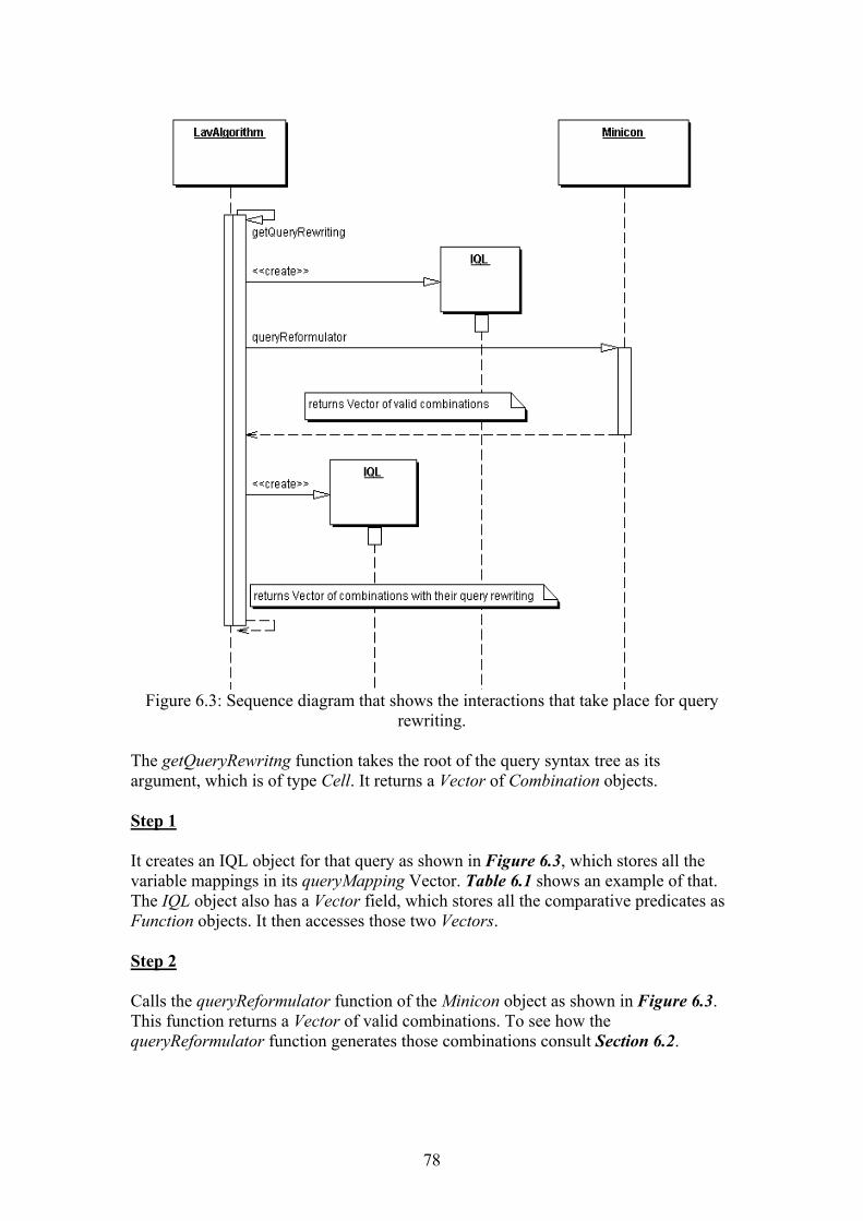
Transcript
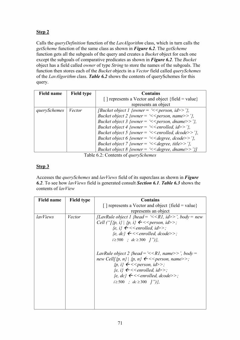
Imperial College of Science, Technology and Medicine
(University of London) Department of Computing
Data Integration System based on both GAV and LAV query processing approaches.
Supervisor: Dr. Peter McBrien
Second Marker: Dr. Khalil Amiri
By Apurba Dey
Submitted in partial fulfilment
of the requirements for the MSc Degree in Advanced Computing of the
University of London and for the Diploma of Imperial College of
Science, Technology and Medicine.
September 2004
Summary Data Integration is the process of combining data residing at different sources with associated local schemas to form a single virtual database with an associated global schema [1, 2]. This is to provide the user with a uniform query interface for multiple independent heterogeneous data sources [3, 4]. There are four main approaches of data integration. They are Global As view (GAV), Local As View (LAV), Global Local As View (GLAV) and Both As View (BAV). BAV is known as the best data Integration approach as it does not have any of the drawbacks of GAV, LAV and GLAV approaches. The unique feature of the BAV is that the constructs of global schema can be extracted as views over the sources (feature of GAV) and the constructs of sources can also be extracted as the views over the global schema (feature of LAV). Therefore, it is possible to implement both the GAV and LAV based query processing approaches for a BAV based data integration system. AutoMed is the first data integration system based on the BAV approach. Currently it uses the feature of the GAV that BAV approach supports for query processing. However, the GAV based data integration systems cannot derive the global schema constructs that do not have equivalent source schema constructs, as views over the sources. Therefore, they cannot answer any queries on those global schema constructs. However, the LAV based systems can derive some of the source schema constructs as views over those constructs of the global schema. Therefore, they can answer any queries on those global schema constructs. On the other hand, the LAV based data integration systems cannot derive the source schema constructs that do not have equivalent global schema constructs, as views over the global schema. Therefore, they cannot answer any queries on those source schema constructs. However, the GAV based systems can derive some of the global schema construct as views over those constructs of the sources. Therefore, they can answer any queries on those source schema constructs. So, a Data Integration system based on both approaches would not have the drawbacks of both the GAV and LAV based data integration systems. Currently, there is no data integration system based on both of these approaches. Therefore, it is decided to use the feature of LAV that is supported by the BAV approach to implement a LAV based query processing approach. Then, we can combine the result of both the existing GAV approach and the LAV approach to answer users query. Currently existing LAV based data integration systems uses bucket and inverse-rule algorithm to deal with large numbers of LAV views. Both of these algorithms have drawbacks. Therefore, it is decided to use the Minicon algorithm, which is implemented only for the experimental purposes. The results of the experiment showed that it is the best-performed algorithm for this purpose.
2
However, so far this algorithm is defined in terms of datalog notation and AutoMed is based on IQL. Therefore, it is decided to define the algorithm in terms of IQL before implementing it. In order to fulfil the objectives of this study, the following things are achieved.
• The Minicon algorithm is defined in terms of IQL, which is entirely innovative.
• The Minicon algorithm is implemented, which is not used by any of the
existing LAV based systems.
• The LAV approach based on Mincion algorithm is implemented, using the feature of LAV that is supported by the BAV approach, which is also never been done before.
• Both the GAV and LAV approach is used to answer user query, which is also
innovative.
3
Acknowledgements I would like to express my thanks and gratitude to my Project Supervisor, Dr. Peter McBrien, for his advice, support and guidance throughout my dissertation. I would also like to thank my second marker Dr. Khalil Amiri and Nikos Rizopoulos, who have been an invaluable source of advice. Lastly, I would also like to say thanks to all my friends and family who have kept my spirits high, especially during the difficult times.
1.1 Motivation…………………………………………………………... 8 1.2 Our objectives………………………………………………………. 8 1.3 Outline of the chapters………………………………………………
9
Chapter 2 Background (1) – Data Integration………………………………. 10 2.1 Basic concepts of Data Integration…………………………………. 10 2.2 Components of Data Integration……………………………………. 11 2.3 overview of conjunctive queries and datalog notations…………….. 11 2.4 Global As View (GAV) approach…………………………………... 12
2.4.1 Example of GAV…………………………………………. 12 2.4.2 Pros and cons of GAV approach………………………….. 13 2.4.3 Overview of different GAV mappings……………………. 14 2.4.4 Overview of systems based on GAV approach…………... 15
2.5 Local As View (LAV) approach……………………………………. 16 2.5.1 Example of LAV………………………………………….. 16 2.5.2 Pros and cons of LAV approach………………………….. 16 2.5.3 Overview of different LAV mappings……………………. 17 2.5.4 Overview of systems based on LAV approach…………… 18
2.5.4.1 Bucket algorithm……………………………….. 18 2.5.4.1.1 An example of this algorithm…………. 19 2.5.4.1.2 Advantages of this algorithm…………. 21
2.5.4.2 Inverse-rules algorithm…………………………. 21 2.5.4.2.1 An example of this algorithm…………. 21 2.5.4.2.2 Advantages of this algorithm…………. 23
2.5.4.3 Minicon algorithm………………………………. 23 2.5.4.3.1 An example of this algorithm…………. 25 2.5.4.3.2 Advantages of this algorithm…………. 26
2.6 Global Local As View (GLAV) approach………………………….. 26 2.7 Both As View (BAV) approach…………………………………….. 26
2.7.1 Example of BAV………………………………………….. 28 2.7.2 Advantages of BAV approach……………………………. 29 2.7.3 Overview of system based on BAV approach…………….
30
Chapter 3 Background (2) AutoMed – A Data Integration Framework ….. 32 3.1 Features of AutoMed in general…………………………………….. 32 3.2 Overview of AutoMed Repositories………………………………... 33
3.2.1 Overview of MDR………………………………………... 33 3.2.2 Overview of STR…………………………………………. 34
3.3 Overview of IQL……………………………………………………. 34 3.3.1 Why IQL used in preference to datalog notations………... 35 3.3.2 Representation of IQL queries in AutoMed Framework…. 35
3.4 AutoMed Schema integration and transformations………………… 36 3.4.1 An example schema integration and transformation……… 37
3.5 View generation in this framework………………………………... 40 3.5.1 GAV view generation…………………………………… 40
5
3.6 Query processing……………………………………………………
42
Chapter 4 Problem domain – our objectives………………………………… 43 4.1 Limitations of the GAV based data integration system…………….. 43 4.2 Limitations of the LAV based data integration system……………... 43 4.3 Data integration system based on both GAV and LAV approach….. 43 4.4 Requirement specification…………………………………………... 44 4.5 Our objectives in summary………………………………………….
5.2.1 How Minicon works with IQL queries…………………… 49 5.2.1.1 Definition of this algorithm in terms of IQL……. 49 5.2.1.2 Express datalog query in terms of IQL in general 50 5.2.1.3 Example of this algorithm in terms of IQL……... 51
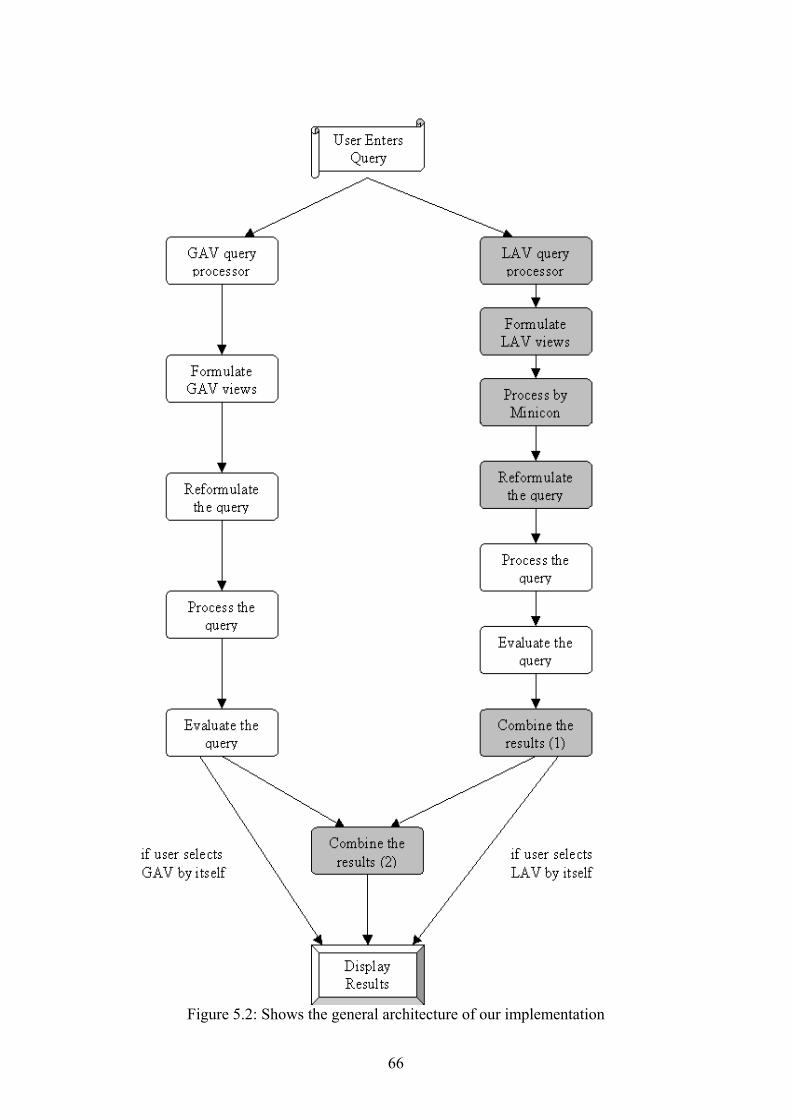
5.3 Query rewriting……………………………………………………... 61 5.4 Combining the result of GAV and LAV……………………………. 61 5.5 General architecture………………………………………………… 64
Chapter 6 Implementation……………………………………………………. 67 6.1 Implementation details for LAV view generation………………….. 67 6.2 Implementation details for Minicon algorithm……………………... 69 6.3 Implementation details for query rewriting………………………… 77 6.4 Implementation details for combining the results of GAV and LAV 80 6.5 Implementation details for query processing component of AutoMed………………………………………………………………...
82
6.6 Implementation overview of the classes…………………………….
83
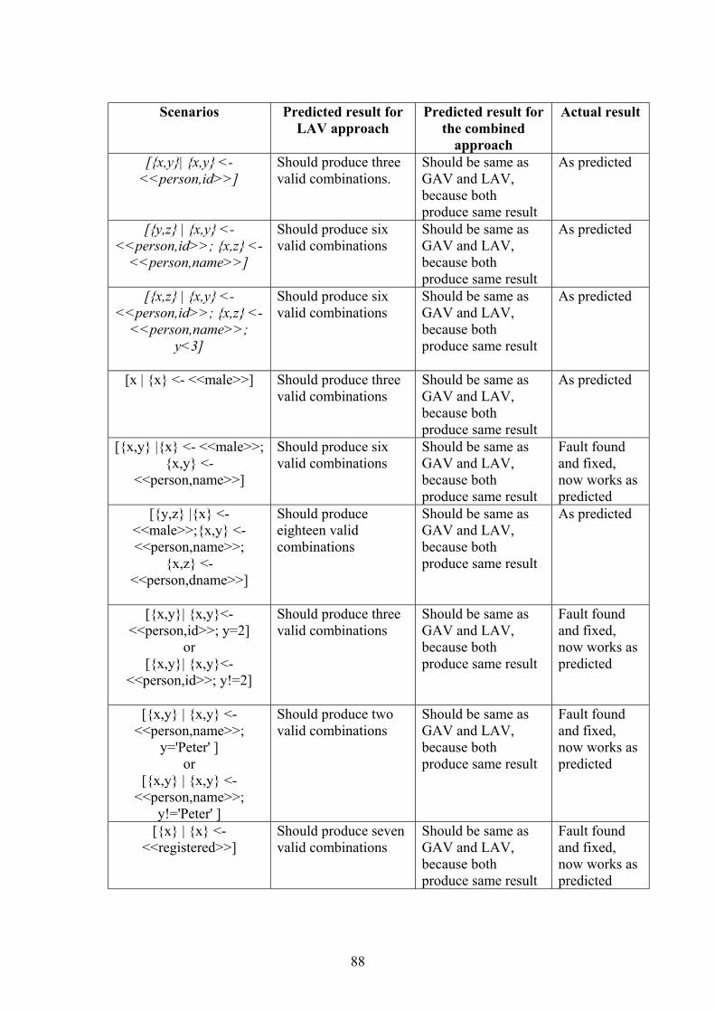
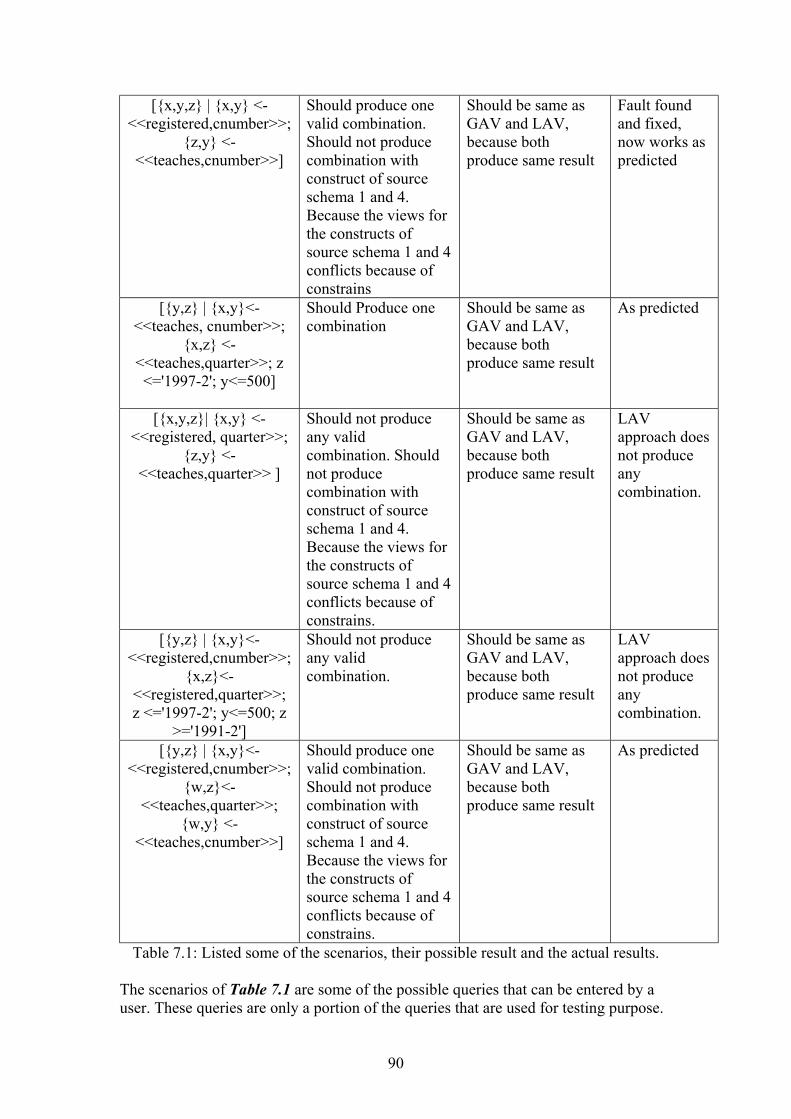
Chapter 7 Testing……………………………………………………………… 87 7.1 White box testing…………………………………………………… 87 7.2 Black box testing……………………………………………………
87
Chapter 8 Evaluation…………………………………………………………. 92 8.1 Effectiveness of the Minicon algorithm……………………………. 92 8.2 Effectiveness of our system in terms of query answering………….. 93 8.3 Other advantages of our system……………………………………..
94
Chapter 9 Conclusion and Future work……………………………………. 95 9.1 Problems we faced………………………………………………… 96 9.2 Limitations………………………………………………………… 96 9.3 Future work………………………………………………………... 97 9.4 Extending our work to implement bucket algorithm……………… 98 9.5 Other possible extensions………………………………………….
101
Bibliography…………………………………………………………………..
102
Appendix A…………………………………………………………………… 106 A1 University example schemas……………………………………… 106 A2 University example data…………………………………………… 106
6
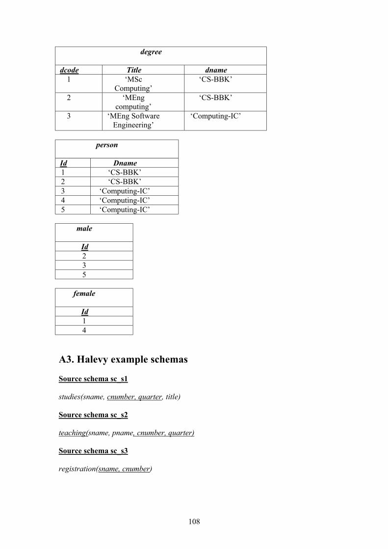
A3 Halevy example schemas…………………………………………… 108 A4 Halevy example data………………………………………………..
109
Appendix B…………………………………………………………………….
111
Appendix C……………………………………………………………………. 112 C1 Quick start guide users of Doc machines under Linux…………….. 112 C2 Quick start guide for other users……………………………………
Introduction The aims of this project is to implement a LAV based Data Integration approach on AutoMed system and find a way of combine the result from both the existing GAV approach and that. 1.1 Motivation The major issue of data integration system based on GAV (Global As View) approach is that it cannot answer queries on the global schema constructs, which is not in its source/local schemas [38, 45]. However, data integration system based on LAV can answer those queries, because it can derive views over those global schema constructs for the constructs of its sources [45]. Similarly, the major issue of data integration system based on LAV (Local As View) approach is that it cannot answer queries on the local schema constructs, which is not in its global schema [38, 45]. However, data integration system based on GAV can answer those queries, because it can derive views over those local schema constructs for the constructs of its global schema [45]. However, a data integration system based on both of these approaches can solve the issues of both approaches. Whenever the GAV approach is unable to answer a query, it can use the result of its LAV approach and whenever the LAV approach is unable to answer a query, it can use the result of its GAV approach. None of the existing data integration system uses both of these approaches to answer a user query. This is influenced us to find a way of combine the result from both these approaches. 1.2 Our objectives The current implementation of the AutoMed system supports GAV approach only. Therefore, we need to implement the LAV approach on AuToMed first. Then find a way to combine their results to answer user query. This is further discussed in Chapter 4.
8
1.3 Outline of the following chapters The report consists of the following structure.
• Chapter 2: This is a background chapter. It outlines the basic concepts of Data Integration system. It describes the four main approaches of data integration and their pros and sons. It mainly focused on LAV approach in particular and described how it is implemented by existing LAV based system.
• Chapter 3: This is the second background chapter. It outlines the features of
AutoMed system. It provides an account of IQL, which is used by the AuToMed system. It also provides an account of AutoMed Schema integration and transformations.
• Chapter 4: This chapter looks into the problem domain and analyses the
requirements, which also defines our objectives.
• Chapter 5: This chapter outlines the design of the various components of our implemented product. It outlines the approaches that are taken to implement those components. It also describes why those approaches are taken in preferences to other alternatives.
• Chapter 6: This chapter provides an account of the implementation details.
This chapter describes how each component is programmed using the logic described in Chapter 5.
• Chapter 7: This chapter provides an account of the testing that our
implemented product has gone through.
• Chapter 8: This chapter provides an account of the effectiveness of our implemented product.
• Chapter 9: This is the conclusion chapter. It outlines the limitations of our
product and some implications for future work
9
CHAPTER 2
Background (1) – Data Integration In recent years large organisations tends to have several databases within them and the internet made it possible to access those different databases, which means there are considerable interest in construction of Distributed Database (DDB) Systems. One of the complex types of DDB is a Heterogeneous Database (HDB), in which there are multiple databases, which has both physical (e.g. managed by different types of DBMS, has different query processing algorithm and concurrency control of transaction manager etc) and semantic (e.g. different local databases model the same real world information using different schema constructs) heterogeneity. Currently the major issue in databases is the integrating those multiple independent heterogeneous databases. This is a major research area both from a formal and from a practical point of view in the last two decades [6, 7, 8, 9, 10, 19]. In recent years, integration is essential for data sources on the web as corporations attempt to provide their customers and employees a consistent view of the data associated with their enterprise and most of the research on integration has focused on Data Integration [3, 19, 20]. 2.1 Basic Concepts of Data Integration Data Integration is the process of combining data residing at different sources with associated local schemas to form a single virtual database with an associated global schema [1, 2]. This is to provide the user with a uniform query interface for multiple independent heterogeneous data sources [3, 4]. The advantage of Data Integration is that users do not need to find data sources relevant to a query interact with each in isolation and manually combine data from each source. As we can see from Figure 2.1 that user query posed on the Data Integration system is first formulated in terms of the global schema in order to execute. The system then translates it into sub queries, which is expressed in terms of local schemas of multiple independent data sources. Examples of Data Integration applications are enterprise integration, Data Warehouse, Data mining, querying multiple sources on the World Wide Web and data integration of different scientific experiments, where the sources may be traditional databases, legacy systems, csv or structured file [3, 21].
10
Figure 2.1: Basic architecture of Data Integration system.
2.2 Components of Data Integration There are two main components of Data Integration. They are as follows:
• Schema Integration: concerned with how the schemas of various local databases may be combined into a single global schema.
• Query Processing: concerned with how a query may be answered by being
translated to one or more queries on source databases. There are four main approaches of Data Integration. They are Global As view (GAV), Local As View (LAV), Global Local As View (GLAV) and Both As View (BAV). These approaches uses view definitions to specify the mapping between local and global schemas. A view definition is query over other constructs to define the extents of a construct. These mappings are used to translate queries expressed in terms of global schema to sub queries expressed in local schemas. 2.3 Overview of conjunctive queries and datalog notations For the rest of the sections, we are going to use datalog notations to express view definitions and queries. Hence, here we provide a brief reminder of datalog notation and conjunctive queries [29, 30].
11
A conjunctive query has the form: Where q and refers to predicate names. The predicate names refer to database relations. The atom is the head of the query and the atoms are subgoals in the body of the query. The tuples is either variables or constants.
).(,),........(:)( 11 nn XrXrXq −
nrr ,........,1
),........( 11 Xr
nXXX ,........,, 1
nrr ,........,1
)(Xq )(, nn Xr
Arithmetic comparisons such as etc may also be appeared as subgoal of a comparison predicate in the query. However, if a variable X appears in a subgoal of a comparison predicate, then X must also appear in an ordinary subgoal.
≠=≤ ,,,p
Conjunctive queries are able to express select-project-join queries. Join predicates of SQL are expressed by multiple occurrences of same variable in different subgoal of the body. Union is also expressed by allowing a set of conjunctive queries with the same head predicate. For example, we will rewrite the following SQL query on the global schema of Figure 2.2 in the conjunctive queries notation.
select enrolled.id, degree.title, degree.dtype, degree.dname from enrolled, degree
where degree.dcode = enrolled.dcode and degree.dype = ‘UG’ Conjunctive query notation is as follows: q( id, title, dtype, dname ): - degree( dcode, title, dtype, dname), enrolled(id, from, to,
dcode), dtype = ‘UG’. A datalog query is a set of conjunctive queries, except that the predicates in the body of the rule do not have to be database relations. It distinguishes EDB (extensional database) predicate referring database relations from IDB (intensional database) predicate referring intermediate computed relations. EDB predicates only appear in the body of the rule whereas IDB predicates appear anywhere. 2.4 Global As View (GAV) approach In GAV, the global schema is defined as views over the local schemas. More precisely, for every construct/element of the global schema is defined by the view over the associated data sources. So, the data residing at the sources provides the meaning of the constructs of the global schema. 2.4.1 Example of GAV Figure 2.2 shows example of local, union and global schemas. These example schemas are inspired from [18]. These schemas will be used through out the report.
12
Figure 2.2: Example of source, union and global schemas. Lets define the GAV definition for the construct GS: degree in Figure 2.2. Considering all four source schemas in Figure 2.2 we get, GS: degree (dcode, title, dtype, dname): - : degree (2LS dcode, title, dtype, deptname)
, : degree (3LS dcode) , : degree (4LS dcode).
2.4.2 Pros and cons GAV approach GAV is effective where a Data Integration system is based on a stable set of sources [2]. It favours the system to carrying out query processing because view definitions tell how to use the sources in order to retrieve data [2]. Therefore, Query processing can be based on some sort of unfolding. Figure 2.3 shows an example of unfolding process. However, extending the system with a new source is problematic because the new source may have an impact on the view definitions of the global schema constructs [2]. In terms of query answering, GAV cannot answer some of the queries. Because it does not deal with the case, when the global schema contains details that is not in the sources [38, 45]. However, the transformation rules for the construct of the local schema can be defined over those details of the global schema (LAV approach see Section 2.5). These transformations have no inverse. So there is no GAV rule for this [45].
13
In order to show an example of that we need to do slight changes to the local schema in Figure 2.2. The modified is as follows. 2LS 2LS
Lets consider the sou2.2 and the modified schema construct dep
Therefore, there is nocannot answer the qufrom the GAV rules oThis example is furth However, sometimesBecause GAV approanot in the global sche 2.4.3 Overview It is important to undno constraint GAV mmappings.
rce schemas , , and the global schema GS of Figure local schema . Now we are in a situation where the global t(uname, cmname) is not in any of the sources.
1LSLS
3LS 4LS
2
Figure 2.3: Example of unfolding process.
way to derive instances of dept from the sources. Therefore, we ery “the campus names of all the degree courses are taught”, n those sources, despite the information being present in . er discussed in Section 5.4.
2LS
GAV approach can answer queries that LAV approach cannot. ch deals with the case when the sources contain details that is ma [38, 45]. Section 2.5.2 shows an example of that.
of different GAV mappings
erstand the difference between exact and sound, constraint and apping, before we look at combination of different GAV
14
An exact GAV mapping means the view definition over the source schemas for a construct of the global schema is exact. Therefore, the extensions of the construct are exactly the set of tuples of objects specifying the corresponding view. On the other hand, a sound GAV mapping means the view definition over the source schemas for a construct of the global schema is sound. Therefore, the set of tuples of objects satisfying the corresponding view is the subset of the extensions of the construct. Constraints refer to integrity constraints such as primary key or foreign key constraint in the global schema.
• No constraint and exact mapping: with no constraint the retrieved global databases would be legal with respect to the global schema [2]. Also there is only one retrieved global database, since the retrieved global database has all the tuples for the corresponding construct in the global schema [2]. This is possible because of the exact mapping. This database is both legal with respect to the global schema and satisfies the mapping with respect to the source database. Therefore, this database would not produce any incompleteness and inconsistency.
• No constraint and sound mapping: as before, the retrieved global database
would be legal with respect to the global schema. However, because of the sound mapping there would be more than one retrieved global database, which may produce incompleteness but no inconsistency [2].
• Constraint and exact mapping: because of the exact mapping there is only
one retrieved global database that satisfies the mapping with respect to source database. However, because of integrity constraint it may be the case that the retrieved global database is not legal with respect to global schema [2].
For example, if we have a query “get the dcode of the enrolled students” on the global schema of Figure 2.2. Now if the retrieved global database contain the tuples [{G500, IT, BSc, Computer Science}, {G750, Computing, BSc, Computer Science}] and [{1, 20Aug99, 20Aug02, G500}, {2, 01Aug99, 03Sep02, G400}] for the relation degree and enrolled of the same global schema, then the retrieved database violates the foreign key constraint. Because, according the foreign key constraint, enrolled [dcode] required to be the subset of degree [dcode]. Therefore, the retrieved global database is inconsistent.
• Constraint and sound mapping: because of the sound mapping there is
more than one retrieved global database that satisfies the mapping with respect to source database [2]. So it can cause incompleteness. However, integrity constraint in global schema can cause inconsistency [2].
2.4.4 Overview of systems based on GAV approach
• Data Warehouse System: pre-compute the queries that might be posed on the system and stored in the global database in order to accelerate the access
15
to data stored on different sources [22]. In order to do that it uses GAV approach to define the constructs of global schemas using views over the sources, compute them and store them in global database.
• Federated Database and Mediator System: data is only materialised in
local schemas [23]. Queries posed on the global schema need to be rewritten in order to execute on one or more local schemas. Examples of mediator systems are TSIMMIS [24], Garlic [25], Coin [26] and Squirrel [27].
• System with integrity constraints: IBIS [21] system is based on GAV
approach that allows integrity constraints in the global schema and also assume views are sound. Generally query answering is very simple in GAV approach, which involve unfolding (Section 2.3.2) strategy. However, this strategy is not sufficient for providing all correct answers in the presence of integrity constraint. IBIS deals with this issue using a logic program. As it is irrelevant from our objectives, it is not discussed any further.
2.5 Local As View (LAV) approach In LAV, the local schemas are defined as views over the global schema. More precisely, for every construct/element of the local schema is defined by the view over the global schema. 2.5.1 Example of LAV Lets define the LAV definition for the construct : degree in Figure 2.2. Considering the global schemas in Figure 2.2 we get,
2.5.2 Pros and cons of LAV approach LAV is effective where a Data Integration system is based on a stable well-established Global schema [2]. It favours the extensibility of the system since adding a new source means simply defining the mapping between it and global schema without any other changes [2]. However, the query processing in LAV is problematic because it involves query reformulation complex [2]. As we can see from the example of Section 2.5.1 that the LAV rule does not directly tell how to use the sources in order to retrieve data. Also LAV does not support evolution of global schema. Adding a construct in the global schema may indeed have an impact on the definition of various elements of source schemas, whose associated views need to be redefined [2].
16
In terms of query answering, LAV cannot answer some of the queries. Because it does not deal with the case, when the source contains details not present in the global schema [38, 45]. However, the transformation rules for the construct of the global schema can be defined over those details of the sources (GAV approach see Section 2.4). These transformations have no inverse. So there is no LAV rule for this [45]. In order to show an example of that we are going to use all the local schemas except
and the global schema of Figure 2.2. However, we need to slightly modify the person relation of the global schema. The modified person relation is as follows.
1LS
person(id, name, sex, dname#)
Now the detail about which course (‘UG’ or ‘PG’) a student enrolled for is not available in the global schema. Therefore, there is no way we can define instances of ug_student of schema and pg_stusent of schema . Therefore, we cannot answer the query “the name of students enrolled to different courses”, from the LAV rules on the global schema, despite the information being present in and . This example is further discussed in Section 5.4.
3LS 4LS
3LS 4LS
2.5.3 Overview of different LAV mappings It is important to understand the difference between exact and sound, constraint and no constraint LAV mapping, before we look at combination of different LAV mappings. An exact LAV mapping means the view definition over the global schemas for a construct of the source schema is exact. Therefore, extensions of the construct are exactly the set of tuples of objects specifying the corresponding view. On the other hand, a sound LAV mapping means the view definition over the global schema for a construct of the source schema is sound. Therefore, the extensions of the construct are the subset of the tuples of objects satisfying the corresponding views. Constraint and no constraint have same meaning as discussed in Section 2.4.3.
• No constraint and exact mapping: sources are views here and answering
queries based on the available data in these views. There may not be any retrieved global database in this case because of inconsistencies in the sources [2].
For example, if there is a exact mapping between : enrolled(id, from, to, dcode) and GS : enrolled(id, from, to, dcode), : enrolled(id, from, to, dcode) and GS : enrolled(id, from, to, dcode) of Figure 2.2, then according to the mapping, the two source relations should contain exactly the same extensions. If they have different extensions, then none of them would satisfy the mapping with respect to source database and would result no retrieved global databases.
3LS
4LS
17
The retrieved global databases would be legal with respect to global schema, because of no constraint [2].
• No constraint and sound mapping: as before, the retrieved global databases
would be legal with respect to the global schema. However, it has incompleteness, which comes from the sound mapping [2].
• Constraint and exact mapping: it is very obvious that LAV with constraint
and exact has inconsistence because we know retrieved global databases of LAV with no constraint and exact has inconsistency. However, there are possibilities of more than one retrieved global database, which satisfies the mapping with respect to the source database. But only some of them are legal with respect to global schema [2]. The reason is the global schema has primary and foreign key integrity constraints in this case.
• Constraint and sound mapping: it is also obvious to say that LAV with
constraint and sound mapping has incompleteness because we know that the retrieved global database of LAV with no constraint and sound has incompleteness. However, there are possibilities of more than one retrieved global database. However, they will only produce incomplete answer [2]. There are also possibilities of inconsistency among the retrieved global databases because of integrity constraint [2]. Section 2.4.3, GAV with constraint and exact mapping, has an example showing how integrity constraints on global schema cause inconsistency.
2.5.4 Overview of systems based on LAV approach As we can see from (Section 2.5.3) that in LAV approach there is more than one possible rewriting for the same query and most of the times there are large number of view definitions, which causes the number of rewritings to be exponential in the size of the query [3]. Previous systems based on LAV approach have mainly used two algorithms in order to deal with large numbers of view definitions. They are the bucket algorithm, which is developed in the context of the Information Manifold system [28] and the inverse-rules algorithm, developed and used in the InfoMaster System [33]. Another algorithm called minicon was first introduced by [32]. So far no LAV based Data Integration system used this algorithm. In all these algorithms, queries are expressed in datalog notations (section 2.3). The following sub-sections provide a brief description of each algorithm and their advantages. 2.5.4.1 Bucket Algorithm The main idea underlying this algorithm is that it considers each subgoal in the query in isolation and determines the view relevant to the subgoal in order to reduce the number of query rewriting that need to be considered. We will see an example of this
18
algorithm in the next sub-section; lets first see what are the two steps of this algorithm? In the first step, it creates a bucket for each subgoal except the subgoal of a comparison predicate in the query. Each entry of the bucket is the head of a LAV rule / definition. However, each entry must satisfy the following conditions.
1a. One of the subgoal of the LAV rule must mapped to a owner of a bucket (a subgoal of the query).
1b. If a head variable of the query appears in the query subgoal, it must also appear in the head of the LAV rule, providing the rule satisfies condition 1a.
1c. If the query has a subgoal of comparison predicate, then any LAV rule with a comparison predicate with the same variable is acceptable if it’s comparison predicate mutually consistent with the comparison predicate of the query, providing the rule satisfies condition 1a and 1b.
1d. If a subgoal of the query mapped to more than one subgoal of a particular LAV rule, then head of this rule appears multiple times in the bucket of that subgoal.
In the second step, it creates a rewriting using combination of one entry from each bucket. Each combination must satisfy the following conditions.
2a. If there is a shared variable in the subgoal of the query, it must also be in the head of the LAV rule; otherwise, the head of the LAV rule must be in the buckets of all the query subgoals that have this shared variable as well.
2b. If a combination contains two LAV rules, if they have comparison predicates, then these predicates must be mutually consistent, providing the combination satisfies condition 2a.
2c. If a combination contains two rules, for example say r1 and r2, where r1 covers query subgoal 1, 2 and r2 covers query subgoal 1, 2, 3. Then, instead of using combination of r1 and r2 as query rewriting, use r2 only.
2.5.4.1.1 An Example of this algorithm Lets consider the following query based on the global schema in Figure 2.2. Q(I, N, T, DN) : - person(I, N, S, C, DN), enrolled(I, F, TO, DC),
degree( DC, T, DT, DN), , 500≥I 200≥DC
Now lets consider the following LAV rules. R1(id, name, dname, from, to) : - person (id, name, sex, course, dname),
Table 2.1: Contents of buckets. The rule R6 is not included in any of the buckets in Table 2.1, because the subgoal of the rule cannot be mapped to any of the owner of the bucket. Therefore, it does not satisfy the condition 1a (Section 2.5.4.1). The rule R4 is not included in the bucket of person(id, name, sex, course, dname) because the head variable name of query is in the domain of this subgoal and it is not in the head of rule R4. Therefore, it does not satisfy the condition 1b (Section 2.5.4.1). The rule R3 is not included in the bucket of person(id, name, sex, course, dname) because the comparison predicates and are mutually inconsistent.
Therefore, it does not satisfy the condition 1c (Section 2.5.4.1).
500≥id 400≤id
In the second step, a entry from each bucket are combined to form the query rewriting. The possible combinations are as follows. R1, R1, R2 = R1, R2 by condition 2c (Section 2.5.4.1). R1, R1, R4 = R1, R4 R1, R1, R5 = R1, R5 R1, R2, R2 = R1, R2 R1, R2, R4 = R1, R4 or R1, R2 R1, R2, R5 R1, R5, R2
20
R1, R5, R4 R1, R5, R5 = R1, R5 However, the query rewriting is as follows. Q(I, N, T, DN) : - R1(id, name, dname, from, to),
R2(id, dcode, title, dname)
Any combination with R1 and R5 is not useful because their comparison predicates and are mutually inconsistent. Therefore, it does not
satisfy the condition 2b (Section 2.5.4.1) and produces empty result.
300≥dcode 250≤dcode
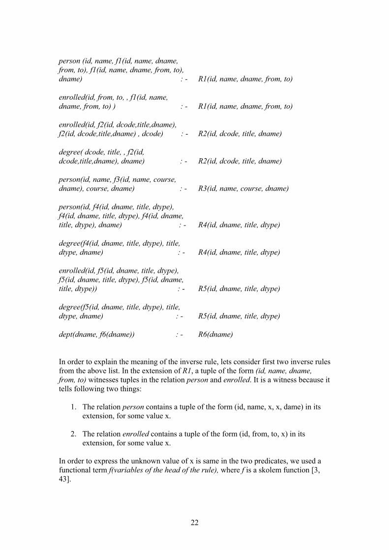
On the other hand, combination of R4 is not useful because the head of the rule does not contain this shared variable dcode of relation degree. So, it requires to cover the subgoal enrolled as well, because it is the other subgoal contain the shared variable dcode. Therefore, it does not satisfy the condition 2a. 2.5.4.1.2 Advantages of this algorithm The main strength of this algorithm is that it exploits the subgoals of the query to cut significantly the number of possible rewriting that need to be considered. A check to see whether a rule should belong to a bucket can be done in polynomial time in the size of the query and LAV rule when the predicates involved are arithmetic comparisons [3]. The algorithm can be extended in cases where the query (not the rules) is a union of conjunctive queries and query involving other form of predicates such as class hierarchies [36]. Finally, Also it is possible to identify interleaving optimisation and execution in this algorithm when a bucket contains large number of rules [36]. 2.5.4.2 Inverse-rules Algorithm The inverse-rules algorithm is also developed in the context of Data Integration system [33]. The main idea underlying this algorithm is that it inverts the LAV rules. Therefore, the inverted LAV rules (like GAV Section 2.4) directly shows how to compute tuples for the global schema relations from the tuples of the relations of the source schemas (head of the LAV rules). The next section shows an example of this algorithm. 2.5.4.2.1 An example of this algorithm Considering the query and LAV rules in Section 2.5.4.2.1, we construct one inverse rule for each subgoal (except comparison predicates) in the body of the LAV rules as follows.
dept(dname, f6(dname)) : - R6(dname) In order to explain the meaning of the inverse rule, lets consider first two inverse rules from the above list. In the extension of R1, a tuple of the form (id, name, dname, from, to) witnesses tuples in the relation person and enrolled. It is a witness because it tells following two things:
1. The relation person contains a tuple of the form (id, name, x, x, dame) in its extension, for some value x.
2. The relation enrolled contains a tuple of the form (id, from, to, x) in its
extension, for some value x. In order to express the unknown value of x is same in the two predicates, we used a functional term f(variables of the head of the rule), where f is a skolem function [3, 43].
22
Q(I, N, T, DN) : - person(I, N, S, C, DN), enrolled(I, F, TO, DC), degree( DC, T, DT, DN), , 500≥I 200≥DC
Now, say the rule R1 includes the following tuples for the query. R1{(550, Peter, CS, 25Aug85, 26Aug89 ), (600, Nikos, CS, 20Jul00, 20Jun04), (575, Alex, Ph, 23Aug91, 23Sep95)} The inverse rules would compute the following tuples for the relations connected to rule R1. person{ (550, Peter, f1(550, Peter, CS, 25Aug85, 26Aug89 ), f1(550, Peter, CS, 25Aug85, 26Aug89 ), CS), (600, Nikos, f1(600, Nikos, CS, 20Jul00, 20Jun04), f1(600, Nikos, CS, 20Jul00, 20Jun04), f1(575, Alex, Ph, 23Aug91, 23Sep95), f1(575, Alex, Ph, 23Aug91, 23Sep95), Ph)} enrolled{(550, 25Aug85, 26Aug89, f1(550, Peter, CS, 25Aug85, 26Aug89 ), (600, 20Jul00, 20Jun04, f1(600, Nikos, CS, 20Jul00, 20Jun04)), (575, 23Aug91, 23Sep95, f1(575, Alex, Ph, 23Aug91, 23Sep95))). Similarly, the other inverse rules would compute the tuples for their corresponding relations. These computed tuple would be used to answer the query. In the case a relation is connected to more than one head of LAV rule, for example, person connected to R1, R3 and R4, then a query with a person subgoal would have three possible rewriting. 2.5.4.2.2 Advantages of this algorithm The key advantage of this algorithm is its simplicity and modularity. As we can see from the example in Section 2.5.4.2.1 that the query rewriting is much simpler, because rules tells directly which rules to use for the rewriting. This algorithm can be extended to exploit functional dependencies on the database schema, recursive queries and the existence of access-pattern limitations [37]. This algorithm produces maximally contained rewriting. Unlike the bucket algorithm (Section 2.5.4.1), the inverse rules can be computed once and be applicable to any query. 2.5.4.3 MiniCon Algorithm This algorithm begins like bucket algorithm, considering each LAV rules containing the subgoals that corresponds to subgoals of the query. However, when the algorithm finds a mapping from a subgoal in the query to a subgoal in the body of the rule, it changes perspective and looks at the variables in the query. The algorithm considers the join variables in the subgoals of the query and finds the minimal additional set of subgoals that need to be mapped to subgoals in the body of the LAV rules.
23
This set of subgoals and mapping information is called a MiniCon Description (MCD), which can be viewed as generalised buckets. The first phase of the algorithm creates the MCD’s. In the second phase the algorithm combines the MCD’s for query rewritings. We will see an example of this algorithm in the next sub-section; lets first see the MCD’s and the two phases in more detail. An MCD C for a query Q over a LAV rule R is a tuple of the form ( cccc GYRh ,,)(, ℘ ) where:
• , is a mapping h from variables of R to variables of R. ch
• cYR )( , is the result of applying on rule R, where ch )( Ahc=Y and A is the head variable of R.
• , is a mapping from variables of the subgoals of the query to .
c℘hc )(var Rofiables
• , is a subset of the subgoals in query Q that are covered by the subgoals of a LAV rule.
cG
As we know from the earlier discussion that in the first phase of the algorithm, it creates MCD’s for each LAV rules. An MCD for a rule exists if the rule satisfies the following conditions.
1a. One of the subgoal of the LAV rule must mapped to a subgoal of the query.
1b. If a head variable of the query appears in the query subgoal, then it must appear in the head of the LAV rule, providing the rule satisfies condition 1a.
1c. If the query subgoal has a shared variable (used to do the join with another subgoal), then it must also appear in the head of the LAV rule, providing the rule satisfies conditions 1a and 1b. Otherwise, the MCD for the rule must cover all the query subgoals that contain this shared variable.
1d. If the query has a subgoal of comparison predicate, then any LAV rule with a comparison predicate with the same variable is acceptable if its comparison predicate mutually consistent with the comparison predicate of the query, providing it satisfies conditions 1a, 1b and 1c.
In the second phase, it creates a rewriting using combinations of MCD’s. Each combination must satisfy the following conditions.
2a. The combination covers all the subgoals of the query. In other words, the union of of all MCD’s = subgoals of the query (excluding subgoals MCDGof comparative predicates).
24
2b. The intersection of any two must be , providing the combination MCDG ∅satisfies condition 2b.
2c If a combination contains two MCD’s formed from two LAV rules, if they have comparison predicates, then these predicates must be mutually consistent, providing the combination satisfies condition 2a and 2b.
2.5.4.3.1 An example of this algorithm Lets consider the same query and LAV rules used for the bucket algorithm in Section 2.5.4.1.1. Q(I, N, T, DN) : - person(I, N, S, C, DN), enrolled(I, F, TO, DC),
degree( DC, T, DT, DN), , 500≥I 200≥DC
For simplicity, we query subgoals person(I, N, S, C, DN), enrolled(I, F, T, DC) and degree( DC, T, DT, DN) as 1,2 and 3 respectively. The MCD’s created after the first phase is in Table 2.2 as follows.
id id, name name, sex sex, course course, dname dname, from from, to to, dcode dcode
Id I, name N, dname DN
1
R2(id, dcode, title, dname)
Id id, from from, to to, dcode dcode, title title, dtype dtype,
dname dname
Id I, title T, dname DN
2, 3
R5(id, dname, title, dtype)
Id id, from from, to to, dcode dcode, title title, dtype dtype,
dname dname
Id I, title T, dname DN
2, 3
Table 2.2: MCDs formed from the first phase of this algorithm. As you can see from Table 2.2 that like the bucket algorithm (Section 2.5.4.1), this algorithm does not create an MCD for rule R3 and R6, because the rules do not satisfy the condition 1d and 1a respectively. The most important point is that this algorithm does not create an MCD for R4, because the head of the rule does not contain the shared variable dcode of relation degree and also this rule does not cover the subgoal enrolled. Therefore, it does not satisfy the condition 1c.
25
The possible combinations of MCDs are as follows. R1, R2 R1, R5 However, the valid rewriting is combination no 1. Like the bucket algorithm (Section 2.5.4.1), combination no 2 does not satisfy the condition 2c. 2.5.4.3.2 Advantages of this algorithm As we know from Section 2.5.4.1.2 that the main problem of the bucket algorithm was, the cartesian product of the buckets are very large. As a result second phase of the algorithm has to deal with large number of combinations. Note that, in our example it produces 9 possible combinations. However, MiniCon algorithm produces only 2 combinations in its second phase (Section 2.5.4.3.2). It does that by removing the irrelevant rules from consideration in the first phase of the algorithm, which bucket algorithm does in the second phase. Also, some of the combinations of the bucket algorithm produce duplicate query rewriting, which is not possible in MiniCon. Therefore, it has less combination to deal with for query rewriting, which makes the algorithm more efficient. A detailed set of experiments carried out in [32], which shows that the MiniCon significantly outperforms the inverse-rules algorithm, which in turn outperforms the bucket algorithm. Furthermore, the experiments show that this algorithm scales up to hundreds of rules. 2.6 Global Local As View (GLAV) approach GLAV is extension of LAV rules where the head of the rule may be conjunction of predicates in the query language and may contain free variables that do not appear in the body of the rule. As GLAV is irrelevant to our project, we will not discuss about this approach any further. For further explanation consult [38, 39, 40]. 2.7 Both As View (BAV) approach BAV is a unifying framework of GAV (Section 2.4) and LAV (Section 2.5) and based on reversible schema transformations [1]. The unique feature of BAV is that the constructs of global schema can be extracted as views over the sources and the constructs of sources can also be extracted as the views over the global schema (we will see an example of that later in the section). This is the reason why it is termed as BAV. Schema transformation in BAV involved a sequence of primitive transformation steps such as t , which can be applied to make an incremental transformation. Each primitive transformation makes delta changes to the schema by adding, deleting or renaming one of the schema constructs.
nt,......,1
it
26
These transformations are defined in terms of lower level common data model called Hypergraph-based Data Model (HDM). HDM is used because semantic mismatches between modelling constructs can be avoided and it also provides a unifying semantics for higher-level modelling constructs such as relational, ER, UML and XML data sources [41, 42]. For simplicity, we will use relational data model to show how BAV integrate two sources into one global schema. Therefore, it is important to familiarise with the primitive schema transformations for this data model. In order to define them in terms of HDM, IQL notations are used. See Section 3.3 for an overview of IQL. The HDM definitions for them are as follows:
• , which adds a new relation R with primary keys . The primary key values in the extent of R are specified by query
q in terms of already existing schema constructs.
),,....,,(Re 1 qkkRladd n >><<
1,,....,1 ≥nkk n
• , which adds a non-primary key attribute a to relation R.
The extent of the binary relationship between primary key attributes and the new attribute a is specified by query q in terms of already existing schema constructs.
),,( qcaRaddAtt >><<
• , which deletes a relation R with primary
keys k . The set of primary key values in the extent of R can be restored from the remaining schema constructs, which is specified by query q.
),,....,,(Re 1 qkkRldel n >><<
1,,....,1 ≥nkn
• , which deletes a non-primary key attribute a from the
relation R. The extent of the binary relationship between primary key attributes and a can be restored from the remaining schema constructs, which is specified by query q.
),,( qcaRdelAtt >><<
Note that, all the primitive transformation rules have an argument c, which specifies a constraint on the data that must be hold if the transformation is to apply, which can be used to enforce foreign key constraints. Also all the primitive transformations have a derivable reverse transformation. For example, the reverse transformation of
is del . ),,....,,(Re 1 qkkRladd n >><< ),,....,,(Re 1 qkkRl n >><<
BAV specification uses two more primitive transformations called conRel and conAtt. They behave the same way as delRel and delAtt except that they indicates their query q may only partially restore the extent of the deleted constuct. Those transformations also have corresponding reverse transformation called extRel and extAtt respectively.
27
2.7.1 Example of BAV We will use the sources and global schema of Figure 2.2 to show how BAV approach integrates sources and into one global schema GS . The complete BAV specification for the integration of sources and into GS is as follows.
3LS 4LS
3LS 4LS
(1) addRel(<<person, id>>, {x | x ∈ <<ug_student, id>> ∨
x ∈ <<pg_student, id}) (2) addAtt( <<person, name>>, notnull, {x, y | (x, y) ∈ <<ug_student, name>>
x ∈ <<pg_student, id>>}) (18) delAtt(<<pg_student, sex>>, notnull, {x, y | (x, y) ∈ <<person, sex>> ∧
x ∈ <<pg_student, id>>}) (19) delRel( <<pg_student, id>>, { x | x ∈ <<person, id>> ∧
(x, ‘UG’ ) ∉ <<person, course>>}) As we can see from the above specification that the steps (1) – (5), (6) – (8), (9) – (10), (11) - (12) and (13) are for global schema ( GS ) constructs person, enrolled, degree, dept, campus and university respectively. These steps are same as decomposition of GAV rules. For example, the following GAV rule is decomposed to generate steps (1) –(5). GS :person (id, name, sex, course, dname): - :ug_student( id, name, sex ) 3LS ∨ :pg_student( id, name, sex). 4LS
28
Therefore, it is clear that GAV definition can be used to partially derive BAV definition and BAV definition can be used to fully derive GAV definition. On the other hand, steps (14) - (19) are for the constructs of the sources ( and ). These steps are same as the decomposition of LAV rules. For example, the following LAV rule is decomposed to generate steps (14) – (16).
course =’UG’. Therefore, it is clear that LAV definition can also be used to partially derive BAV definition and BAV definition can also be used to fully derive LAV definition. 2.7.2 Advantages of BAV approach As we can see from Section 2.7.1 that BAV definitions are partially derivable from both GAV and LAV definitions. In other words, Together GAV and LAV definitions fully derive BAV definitions. Therefore, any reasoning or processing, which is possible with the view definitions of GAV and LAV, is also possible with the definitions of BAV. So, BAV combines the benefits of both GAV and LAV. As we can see from Section 2.4.2 that the principle disadvantage of GAV is that it does not support evolution of local schemas. However, BAV supports the evolution of local schemas. So BAV has advantage over GAV. In BAV, schemas are transformed incrementally by applying a sequence of primitive transformation steps . So, if T was the transformation from
, then a new transformation from can automatically be generated by prefixing the reverse of t toT :
ntt ,......,1
gS
old
ni toSSS UUUU ........1 gni StoSSS UUUU ....'....1
old
oldnew Tt ;=T Now there are three cases to be considered for t for the transformation.
1. If t is a add or del transformation, then the new schema is semantically equivalent to . So any information which is derivable form , can also be derived from . Therefore, no changes are required for or T .
'iS
gSiS
'iSiS
new
2. If t is a contract transformation, then some of the information that was present
in , is no longer in . So it may be the case now that contains some constructs, which is no longer be derivable from local schemas. This can be determined automatically through inspection on T . So, these constructs of
and the corresponding extend steps of each of the local schemas from T can be removed.
iS
g
'iS gS
new
S new
29
3. If t is a extend transformation, then the relationship between the new construct and need to be examined, since the new construct may be derivable from
through some transformation. This requires domain knowledge. If the new construct is derivable form , then the transformation step T, need to be appended to T , in order to add the new construct to . If it is not derivable then the extend step need to be appended to T for the same purpose.
gS
gS
gSnew
gSnew
On the other hand, from Section 2.5.2 we can see that the principle disadvantage of LAV is that it does not support evolution of global schemas. However, BAV supports the evolution of global schema as well. So BAV has advantage over LAV. So, if was the transformation from , then a new transformation from can automatically be generated by suffixing t toT :
oldT gni StoSSS UUUU ........1
'gSto........1 ni SSS UUUU
old
T tT oldnew ;= Again there are three cases to be considered for t for the transformation.
1. If t is a add or del transformation, then is semantically equivalent to . So any information which was available from , is also available from . So no change is required for T .
'gS gS
'gS gSnew
2. If t is a contract transformation, then some information, which used to be
present in , is no longer present in . This means does not have representation for some of the local schema constructs now. No change is required for T .
gS 'gS 'gS
new
3. If t is a extend transformation with a void query, then the relationship between
the new construct and local schemas need to be examined. This requires domain knowledge, since the new construct may be partially or completely derivable from . If it is not derivable from , then no further change is required for . Otherwise, the last sep t of T need to be replaced by more informative extend or add step.
nSS ,.....,1
nSS ,.....,1newT
nSS ,.....,1new
2.7.3 Overview of systems based on BAV approach As we discussed in Section 2.7.2, one advantage of BAV over GAV and LAV is that it supports both the evolution of global and local schemas, which includes addition and removal of local schemas. These evolutions can be expressed as extension to the existing pathways. So new view definitions can be generated as required for query processing from the new pathways. This feature of BAV is well suited for P2P Data Integration requirements [46]. In P2P, peers may join or leave the network at any
30
time, or may change their local schemas, published schemas, or pathways between schemas. However, in order to use BAV for P2P, it need to be extended to support that the logical extent of the global schema is the upper bound on the logical extent of the local schema [46]. Therefore, the extend and contract transformation rules of BAV are extended as follows:
• extendT (c, ql, qu), which adds a new construct c of type T to form a new schema s’ from s. Query ql determines the minimum extent of c in s’ (or void if not determined) and qu determines the maximum extent of c in s’ (or Any if not determined).
• contractT (c, ql, qu), which removes a construct c of type T to form a new
schema s’ from s. As before, ql and qu determines the lower and upper bounds of the extent respectively.
31
CHAPTER 3
Background (2) AutoMed – A Data Integration Framework
The Automed is a British EPSRC funded research project, jointly run by Birkbeck and Imperial Colleges, in the University of London. This project has developed the first implementation of Both As View (BAV) Data Integration approach [11]. 3.1 Features of AutoMed in general Figure 3.1 depicts the main components of Automed system. The model definitions tool supports the specification of modelling constructs and primitive transformations of high-level modelling languages in terms of lower-level hypergraph data model (HDM). Model Definitions Repository (MDR) is used to store these definitions [12]. The schema transformation and integration tool supports the creation of intermediate and global schemas from the source schemas using the corresponding transformation pathways. The Schemas & Transformations Repository (STR) is used to store the source, intermediate, global schemas and their transformation pathways [12].
Figure 3.1: The Automed Architecture
The global query processor supports the processing of global queries using the schemas and transformation pathways in the STR. Currently; the query processing in Automed is based on Global As View (GAV) approach [13]. Global queries are first translated into the intermediate query language (IQL), which is then reformulated into distributed queries over sources using GAV views.
32
Global query processor supports optimisation of global query. After the optimisation, it is translated into the query languages supported by the data sources. This is then submitted to the sources for evaluation. The task of schema evolution tool is to support the evolution of schemas and transformation pathways in MDR. The schema evolution tool also automatically simplifies these evolved pathways. For example, ren c c’; del c’ = del c, add c’; ren c’ c = add c and ren c’ c’’; ren c’’ c = ren c’ c [14]. 3.2 Overview of Automed Repositories The core of the Automed repository is the reps java package, which is the platform for other components to be implemented upon. Currently, the reps API uses RDBMS to store data modelling language descriptions in the HDM, database schemas and transformations between those schemas [15]. Two logical components of Atomed repository are Model Definitions Repository (MDR) and Schema Transformation Repository (STR). 3.2.1 Overview of MDR The Model Definitions Repository (MDR) stores the descriptions of modelling languages represented as combinations of nodes, edges and constraints in the HDM [16]. In essence, it has a list of constructs with the arguments to create an instance of each construct and the means by which to translate them into HDM for each modelling languages. Each construct is given an HDM type, which is either of nodal, linkage, link-nodal or constraint. Nodal is an object with extent (typically an entity type) that can exist independently of anything else. Corresponds to an HDM node. A Link is an association between at least two nodal or link objects. Corresponds to an HDM edge between at least two nodes or edges. Link-nodal is a link, which associates some pre-existing nodes or links as well as some new nodes, which are created along with the link. Constraint is a sentence with holes in it, which are filled by instances of the SchemaObject. Each argument needed to create an instance of a construct can be a simple name, a reference to an existing object of a given construct type, a list of alternatives or sequence. Each argument has a lower or upper cardinality, which specifies how many times the name/construct/alternation/sequence, can appear. An example for that would be an ER entity and attribute. An entity is a nodal HDM type and has a construction argument – its name. An attribute is a link-nodal HDM type and has two construction arguments – its name and the existing entity to which it should be linked.
33
3.2.2 Overview of STR The Schema Transformation Repository (STR) stores information about schemas defined in terms of data modelling concepts in the MDR, described in Section 3.2.1 and transformation pathways between them [16]. A schema is a list of objects and their associated object schemes. Each object has reference to an instance of a particular construct in the MDR. Also an object’s scheme directly relate to the instantiation arguments of the object’s construct in the MDR. The first instantiation argument name is used as the name of the object. It is important to note that, schemas themselves have no existing modelling language. Instead, the objects are of some modelling languages through their construct type. Therefore, the transforming a schema from one language to another one involves creating an intermediate schema with some constructs from both languages. There are two types of schema, which are store in STR. They are extensional and intermediate schemas. Extensional schemas are actual data sources. Intermediate schemas are described by looking at another schema’s extension and a pathway of transformations between the two. 3.3 Overview of IQL The Automed Intermediate Query Language (IQL) is a functional language. The main purpose of it is to provide a common query language so that queries written in various high-level query languages such as SQL can be translated into and out of [17]. Constants in IQL can be strings, Booleans and real and integer numbers. There are also variables and identifiers in IQL. IQL also supports tuples e.g. {1,2,3} and lists e.g. [1,2,3]. Lambda abstractions can be used to define anonymous functions. For example, a function adds the components of its argument can be defined as follows.
Lambda {x, y, z} ((+) ((+) x y) z)
Most of IQL’s built-in functions are prefix form apart from the operators ++ and - - denoting list append and monus are infix form. IQL’s comprehensions comprised with head expression followed by a list of filters or generators. Generators iterate a pattern over a list-valued expression, where a pattern is either a variable or a tuple of patterns. Filters are Boolean-valued expressions that act as filters on the variable instantiations generated. An example of list comprehension is as follows.
[{x, y} | x [1,2,3]; y [‘a’,’b’]; (>) x 1]
34
rgeneratos
filte variables
It is straightforward to represent Relational Algebra (RA) expression in the IQL. The project operators are implemented by using a generator, which binds variables to some constructs in the schema. It then returns a new list built from the variables representing the attributes we wish to project. Since, this is a list construct, the order and repetition of variable bindings returned from the data sources is preserved. Union is implemented using the IQL ++ operator. An RA expression based on the global schema of Figure 2.2, for example, U is equivalent to the following IQL expression.
The select, from and where part of an SQL query is represented by the variables, generators and filter part of the IQL. An SQL query on the global schema of Figure 2.2, for example, select id, name from person where id<20 is equivalent to the following IQL expression.
As we can see from the above example that, product is implemented by more than one generator in the IQL list and a join condition by having same variable binding for the join constructs of the schema. For example, it is person in the above example. The SQL keyword distinct can be used in IQL to eliminate the duplicate answers from a list. IQL also provides a number of aggregation functions of SQL, for example, count, max, min, sum, group by etc. 3.3.1 Why IQL used in preference to datalog notation As we can see from the Section 3.3, that IQL provides almost all the SQL functions, which datalog is unable to. Therefore, in AutoMed, IQL is preferred to provide a common query language so that queries written in various high-level query languages such as SQL can be translated into and out of. Also both the list and set semantics can be expressed in IQL. 3.3.2 Representation of IQL queries in Automed framework In Automed, the string representations of IQL queries are parsed to create an abstract syntax tree representation. The non-leaf cells are either apply cells (@) or lambda
35
cells ( ). Apply cell represents left child being applied to the right child. So, the abstract syntax tree representation for query (+) 1 2 as follow
λ
2
(+) 1
@
@ 3.4 Automed Schema Integration and transformations Automed uses BAV schema integration approach to transform the schemas incrementally by applying sequence of primitive transformations. Figure 3.2 illustrates the integration of n local schemas into a global schema GS. nLSLS ,........,1
Figure 3.2: A general AutoMed Schema Integration.
In this framework, each of the local schemas is first transformed into a union schema US . Each of these n union schemas contains the constructs of all the local schemas . They are syntactically identical and this is asserted by an id transformation step of the form between each pair of US and US for each schema construct c. An arbitrary union schema US then selected to be further transformed into the global schema GS.
iLS
):1 c
i
LS1 nLS,........,,:( UScUSid ii + i 1+i
i
There may be constructs in US , which is not derivable from its corresponding . Similarly, some constructs in may not be transferred into US . They are asserted by extend and contract step within the pathway respectively.
i
LSiLS
i i
ii USLS >−
36
3.4.1 An example Automed Schema Integration and Transformation This example will use the example schemas of Figure 2.2. 1 Transformation Pathway 11 USLS >−
Note that the extendTable transformation used in this transformation pathway is a composite transformation. It is same for rest of the transformation pathways. Its definition is as follows.
3.5 View generation in this framework To define a construct c of a schema A in terms of another schema B, the transformation pathway A B need to be considered. The most significant transformations are delete, contract and rename because view definitions may have query involving constructs, which no longer exists after those transformations. These transformations are same as add, extend and rename steps in the reverse pathway B A. These transformations are handled as follows.
• Delete: This transformation has an associated query, which allows reconstructing the extents of the deleted construct. Also any current view definitions involves such constructs are simply replaced by this query.
• Contract: This transformation has an associated upper-bound and lower-
bound query, which allows reconstructing the extents of contracted construct. Also any current view definitions involves such constructs are replaced by one of the query depending on the requirement of complete or sound views.
• Rename: The references to the new constructs replace all the references to
the old construct in the current view definitions.
3.5.1 GAV view generation For GAV view generation, the pathways from global schema to each local schema are retrieved from AutoMed’s metadata repository [18]. There may be other intermediate schemas within those pathways. Each schema is linked to its neighbour schema by a single transformation step. Figure 3.4 illustrates that. The transformation pathway can be represented as a tree and each schema as its node. The transformation tree is traversed from top to bottom in order to derive view definitions for each global schema construct. Initially, the construct itself is its view definition. Then each node in the tree is visited in downward direction and delete, contract and rename transformation steps associating with that construct are handled as described in Section 3.5. However, when a contract step is encountered, its lower-bound query is used for replacement so that sound GAV views are generated. The tree may also have branch. This happens when the same construct appears more than one child schema. In this case, the construct of parent schema is replaced by a disjunction (OR) of the corresponding constructs of the child schemas.
40
Figure 3.4: Transformation Pathway from a global schema to a local schema in ER
model. For example, lets define the GAV view definition for the construct GS: <<person, sex>>. We will use the reverse of the transformation pathways in Section 3.4.1 for this. At first, the pathway GS is processed. The only significant transformation is
1US→
40t , which deletes the construct <<person, sex>>. It’s query replaces the current view definition <<person, sex>>. The resulting intermediate view definition is as follows.
GS: <<person, sex>>: - US : <<lecturer, sex>> ++ US : <<student, sex>> 1 1
As four local schemas are considered, there are four union schemas and US is one of them. Now traversing the pathway US and US , we replace the body of the view definition by
1
11 LS→ 21 US→
([ {x, ‘M’} | x : <<male>>] ++ [ {x, ‘F’} | x : <<female>> ] OR US : <<lecturer, sex>>)
1LS 1LS 2
++ (Void OR US : <<student, sex>>) 2
Now traversing the pathwayUS and US , we replace the body of the view definition by
22 LS→ 32 US→
([ {x, ‘M’} | x : <<male>>] ++ [ {x, ‘F’} | x : <<female>> ] OR Void OR US : <<lecturer, sex>>)
1LS 1LS
3
++ (Void OR Void OR US : <<student, sex>>) 3
Traversing the pathway US and US , we get 33 LS→ 43 US→
41
([ {x, ‘M’} | x : <<male>>] ++ [ {x, ‘F’} | x : <<female>> ] OR Void OR Void OR US : <<lecturer, sex>>)
1LS 1LS
4
++ (Void OR Void OR US : <<ug_student, sex>> OR US : <<student, sex>>) 3 4
Finally, traversing the pathway US , we get our final view definition 44 LS→
([ {x, ‘M’} | x : <<male>>] ++ [ {x, ‘F’} | x : <<female>> ] OR Void OR Void OR Void)
1LS 1LS
++ (Void OR Void OR US : <<ug_student, sex>> OR US : <<pg_student, sex>>) 3 4
3.6 Query Processing As we know from Section 3.1 that the query processing in AutoMed is based on GAV approach. The users query is based on either a scheme of a table or column schema object of the global schema [44]. For example, the following IQL query on the global schema of Figure 2.2.
Each query has one or more subgoal. In this example they are [{x, y} <<person, id>>] and [{x, z} <<person, name>>]. For each subgoal a view generation (see Section 3.5) process takes place in order to define the global schema constructs as views over the sources. When the views are generated, the schemes of the subgoals are simply replaced by the views, in a process called query rewriting. For example, lets consider view1 and view2 are generated for the two schemes <<person, id>> and <<person, name>> respectively. Then the query rewriting process will create the following reformulated query.
[{y, z} | {x, y} view1; {x, z} view2]
This reformulated query is then evaluated to answer users query.
42
CHAPTER 4
Problem domain – our objectives This chapter looks into the problem domain and analyse the requirements to deal with the current problems. It presents the limitations of both the GAV and LAV based data integration systems in terms of query answering, which generates the problem we are trying to solve and defines our objectives. 4.1 Limitations of the GAV based data integration system Data Integration system based on GAV approach defines their global schema constructs as views over the local schemas. This approach has some limitations. We are interested on its query answering issue in particular. When the global schema contains some constructs, which are not in the local schemas, then this approach cannot define those constructs as views over the sources. As a result, any query on those constructs cannot be answered. See Section 2.4.2 for an example. 4.2 Limitations of the LAV based data integration system Data Integration system based on LAV approach defines their local schema constructs as views over the global schema. This approach also has some limitations. One of the limitations is that it cannot answer some queries as well. When a local schema contains some constructs, which are not in the global schema, then this approach cannot define those constructs as views over the global schema. As a result, any query on those constructs cannot be answered. See Section 2.5.2 for an example. 4.3 Data integration system based on both GAV and LAV approach A system based on LAV approach does not have the same query answering issue that the GAV approach has. The reason is LAV approach can define its local schema constructs over those global schema constructs that are not present in the local schemas. Therefore, it is possible for it to answer any queries based on those global schema constructs.
43
Similarly, a system based on GAV approach does not have the same query answering issue that the LAV approach has. The reason is GAV approach can define its global schema constructs over those local schema constructs that are not present in the global schema. Therefore, it is possible for it to answer any query based on those local schema constructs. Therefore, system based on any of these two approaches cannot solve both issues. However, we thought that if a data integration system can be developed, which has options of both ways of query processing then the problem could be solved. We can take the answer of both the GAV and LAV approach and append them. In this way, when GAV approach is unable to answer, we can use the answers of LAV approach and when LAV approach is unable to answer, we can use the answers of GAV approach. None of the publicly available data integration system is based on both of the GAV and LAV approaches and therefore, our aim is to investigate whether the usage of this data integration system can lead to improvements in the effectiveness of the performance of the system in terms of query answering. 4.4 Requirement Specification The requirements for a data integration system based on both GAV and LAV approaches are as follows.
• Implement the GAV approach: As we have only limited amount of time, we have decided to use the existing GAV approach of the AutoMed data integration system (See Chapter 3 for detail). Implementing that from scratch would be waste of time.
• Implement the LAV approach: As the AutoMed system is based on only the
GAV approach, we have decided to implement the LAV approach from scratch.
Existing systems based on LAV approach uses bucket and inverse-rules algorithm to deal with large number of views. However, both of these algorithms have drawbacks.
Bucket algorithm is inefficient, because the first step of the algorithm does not test one of the relevancy tests, which it does in the second step. Therefore, it makes the second step really costly [3]. This is further discussed in Section 5.2. Inverse-rules algorithm also has drawbacks. This algorithm obtains irrelevant query rewritings, which provide irrelevant answer to a query [3]. It is also inefficient, because it does some recompilations [3]. This is further discussed in Section 5.2.
44
Another algorithm called Minicon is introduced for this purpose by [32]. According to [32], it is an improved bucket algorithm and also does not have the drawbacks of inverse-rules algorithm. However, this algorithm is not used by any of the currently existing LAV based data integration system. It is implemented by [32] for experimental purpose only. We decided to implement this algorithm for our LAV approach. However, one problem is that the query language used by AutoMed is IQL. Most of the existing LAV based system uses datalog notations. Also the Minicon algorithm implemented by [32] uses datalog notation. Therefore, our first hurdle is to define this algorithm in terms of IQL, which is never been done before. Then implement this algorithm. Then develop the LAV approach based on that.
• Combine the results of both approach: If we are successful to implement the LAV approach, we decided to combine the results of both GAV and LAV approaches to answer the users query.
4.5 Our objectives in summary We have four objectives. They are as follows.
• Define the Minicon algorithm in terms of IQL. • Implement the algorithm. • Implement the LAV approach based on that. • Produce answer of a query using the results of both GAV and LAV approach.
45
CHAPTER 5
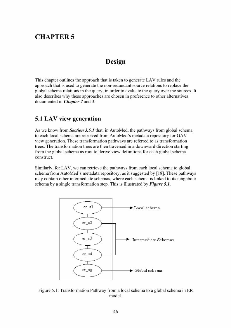
Design This chapter outlines the approach that is taken to generate LAV rules and the approach that is used to generate the non-redundant source relations to replace the global schema relations in the query, in order to evaluate the query over the sources. It also describes why these approaches are chosen in preference to other alternatives documented in Chapter 2 and 3. 5.1 LAV view generation As we know from Section 3.5.1 that, in AutoMed, the pathways from global schema to each local schema are retrieved from AutoMed’s metadata repository for GAV view generation. These transformation pathways are referred to as transformation trees. The transformation trees are then traversed in a downward direction starting from the global schema as root to derive view definitions for each global schema construct. Similarly, for LAV, we can retrieve the pathways from each local schema to global schema from AutoMed’s metadata repository, as it suggested by [18]. These pathways may contain other intermediate schemas, where each schema is linked to its neighbour schema by a single transformation step. This is illustrated by Figure 5.1.
Figure 5.1: Transformation Pathway from a local schema to a global schema in ER
model.
46
According to [18], these transformation trees can be processed in the same way as shown in Section 3.5.1 for GAV view generations, except the source schema end of the tree is taken as the root. According to that each construct’s view definition is the construct itself initially. Then each node of the tree is visited starting from the root in a downward direction and look for delete, contract or rename transformations. When a transformation of this form is encountered it is handled as described in Section 3.5.1. In particular, if a contract transformation step is encountered, any occurrences of the contracted construct within the current LAV view definition is replaced by the upper-bound query accompanying the transformation step, generating sound LAV views. The derivations of LAV views are simpler since there is no branching. The reason for this that there is only one global schema and the views being generated for the constructs of source schema are over this schema. Therefore, there is only single pathway being processed for the source schema. For example, lets define the LAV view definition for the construct : <<female>> in Figure 2.2. We will use the transformation pathways in Section 3.4.1 for this. At first, the pathway is processed. The only significant transformation is , which deletes the construct <<female>>. Its query replaces the current view definition <<female>>. The resulting intermediate view definition is as follows.
1LS
11 USLS → 13t
1LS : <<female>>: - [ x | {x, ‘F’} US :<<lecturer, sex>>] 1
Finally traversing the pathway US , we can see that deletes the construct <<lecturer, sex>>. So replacing the current view definition by its query, we get
GS→1 45t
[x | {x, ‘F’} : <<person, sex>>; member x GS : <<lecturer>> ] GS
Also, deletes the construct <<lecturer>>. Replacing the current view definition with its query, we get our final view definition. This is as follows.
47t
[x | {x, ‘F’} GS : <<person, sex>>; member x [x | {x, y} GS :<<person,
dname>>]]
5.2 Generating combinations of non-redundant source relations for query rewriting The next step is to generate combinations of non-redundant source relations to replace global schema relations in the query, in order to evaluate the query over the sources. As we know from Section 5.1 that the LAV views will be sound in our case. Therefore, there is more than one possible query rewriting for the same query (see Section 2.5.3). Also we know from Section 2.5.4 that most of the time the systems
47
based on LAV has to deal with large numbers of view definitions, which causes the number of rewritings to be exponential in the size of the query. In order to deal with the large numbers of view definitions, previous systems based on LAV approach used mainly the Bucket [28] (Section 2.5.4.1) and inverse-rules [33] (Section 2.5.4.2) algorithm. The advantages of the bucket algorithm (see Section 2.5.4.1.2) attracted us to consider it for this purpose at first. However, this algorithm has some deficiencies. According to [3], the main inefficiency of this algorithm is that in the first step it does not check whether the head of the LAV rule contain the join variable of the query subgoals. As a result, the bucket contains irrelevant head of the rules. Therefore, the Cartesian product of the buckets may be very large. It does this above-mentioned test for each element of the cartesian product in the second step. This testing is
in the size of the query and LAV rules [3]. ∏ −p
complete2
We then considered the inverse-rules algorithm because of its simplicity and modularity (see Section 2.5.4.2.2). However, this algorithm also has some deficiencies. The query rewriting obtained by this algorithm may contain irrelevant source relations, which provides irrelevant tuples to a query [3]. The reason for this is that this algorithm unlike the bucket algorithm (Section 2.5.4.1), does not consider each subgoal of the query in order to compute relevant source relations (heads of LAV rules). Also using these query rewritings for evaluating queries has a significant drawback [3]. The reason is it recomputes the extensions of global schema relations. For example, in Section 2.5.4.2.1, we compute tuples for person and enrolled relation. Now if there is a query, which is a join of those two relations, then, the query need to be evaluated over those relations’ extensions. However, by doing that, we lose the fact that the head of LAV rule already computed the join the query is requesting. We then considered the Minicon algorithm [32] (Section 2.5.4.3). It is a improved bucket algorithm, which solves the limitations of the bucket algorithm and also does not have the drawback of the inverse-rules algorithm. The experiment carried out in [32] showed that it outperforms both the bucket and inverse-rules algorithm. Also, our example in Section 2.5.4.3.1 shows how the first phase of the algorithm eliminates the irrelevant rules from consideration, so that it has to deal with fewer rules in the second phase. So far no limitations of this algorithm is known. Therefore, we reached to a conclusion to use this algorithm to generate combinations of non-redundant source relations to replace global schema relations in the query, in order to evaluate the query over the sources. None of the existing Data Integration system based on LAV used Minicon algorithm. So far it is only implemented for experimental purposes in [32]. Also in [32], the queries were expressed in datalog notation (see Section 2.3). Section 2.5.4.3.1 shows how the algorithm works when the queries are expressed in datalog notation. However, in AutoMed (see Chapter 3) the queries are expressed in IQL (see Section 3.3). The following section shows how the algorithm works when the queries are expressed in IQL.
48
5.2.1 How Minicon works with IQL queries This section describes how we can use Minicon algorithm when the queries expressed in the system are IQL. As there is no Data Integration system exists which uses Minicon with IQL queries, this is entirely innovative work. To illustrate this we will define the Minicon algorithm in terms of IQL queries first. Then we will discuss the general way of expressing a datalog query in terms of IQL. Then we will convert the example in Section 2.5.4.3.1 to IQL in order to both justify our definition and show the changes we need to make to use this algorithm with IQL queries. 5.2.1.1 Definition of the algorithm in terms of IQL As we know from Section 2.5.4.3 that the algorithm has two phases. In the first phase it creates a MCD for each LAV rule. In order to create an MCD for the LAV rules, we are going to follow the following steps.
• Step1: Find out the variables mappings for each subgoal of the query. In AutoMed (see Chapter 3), the query is based on either a scheme of a table or column schema object of the global schema [44]. Therefore, by doing this variable mappings, we actually doing ℘ , a mapping from variables of the subgoals of the query to (see Section 2.5.4.3). This variable mapping also enable us to find out the global schema name of both the head and join variables.
MCD
ofiables )(var RulehMCD
• Step2: Find out the variable mappings for each LAV rule. First we do the
variable mappings using the head of the rule. Then we do the variable mapping using the body of the rule for the same variables. We refer those two mapping as the first phase mapping. The first phase mapping allows us to map the column or table names in the head of the rule to the column or table names in the body of the rule. We refer it as the second phase mapping. The second phase mapping is same as . Therefore, we refer the first and second phase mapping together as mapping for IQL. In order to show how the mapping will be done, lets consider the following LAV rule.
First we do the variable mappings using the head of the rule. In this example they are {R4 d, dname dn}. Then we do the variable mapping using the body of the rule for the same variables. In this example they are {degree d, dname dname}. The first phase mapping allow us to do {degree R4, dname dname}, which is the second phase mapping.
49
• Step3: Find out whether an MCD can be created for each rule. An MCD for a rule exists if the rule satisfies the conditions listed in Section 2.5.4.3. Therefore, this step checks these conditions for each rule to determine that. This step also use the variable mappings discussed in the previous two steps in order to check those conditions.
In the second phase, it generates the combinations of MCDs for query rewritings. Each combination must satisfy the conditions discussed in Section 2.5.4.3. In order to create the valid combinations we are going to follow the following two steps.
• Step1: Generates all the combinations using the MCDs created in the first phase.
• Step2: For each combination check whether it satisfies the conditions
mentioned above. If it does keeps it otherwise, discards it. 5.2.1.2 Express datalog query in terms of IQL in general First we will express a datalog relation in terms of IQL. Then we will express a datalog query and view definition in terms of IQL. In order to do that, we will consider the following datalog relation, query and LAV rule.
Lets start with the relation first. According to Section 3.3 the table / relation name is expressed by inserting the table name within the brackets “<< >>”. Then each column of the relation is expressed separately. The relation name and a column name separated by coma is inserted within the brackets “<< >>”. For example, the datalog relation mentioned above can be expressed in terms of IQL as follows.
<<relation1>>, <<relation1, column1>> and <<realtion1, column2>>
Now lets consider the above mentioned datalog query. Notice that the two relations in the query have same column name column1. This column is used to join the two relations. Also the query is projecting the column2 and column4 columns of the joined relation. According to Section 3.3, the relation and column name is mapped with a variable name in IQL query. The columns responsible for joining two relations are mapped to the same variable. Also, these variables are used for projection. For example, the datalog query mentioned above can be expressed in terms of IQL as follows.
{v, w} <<realation2, column1>>; {v, z} <<relation2, column2>>] Now lets consider the above mentioned datalog view. According to Section 3.3, separate LAV rules need to be defined for the relation and each column of the view. For example, the datalog view mentioned above can be expressed in terms of IQL as follows.
As we can see from the above example that there are two different IQL view definitions are possible for the same datalog view. The Minicon algorithm would produce different combinations using the LAV rules of different view definitions. Therefore, the results would be different for different combinations. Therefore, the results of an IQL query are not directly comparable to the result of a datalog query. 5.2.1.3 Example of this algorithm in terms of IQL First, the query itself needs to be converted from datalog notation to IQL. This is as follows.
Now the views need to be expressed in IQL. We considered the extensions of person for R1 and R3, degree for R2, R4 and R5 and dept for R6. They are as follows. R1a <<R1>> : - [{p} | {p, i} <<person, id>>;
First phase of the algorithm Now we are going to do the first phase of the algorithm. As we know from Section 5.2.1.1 that the first phase has three steps. Step 1 We get the variable mapping for each subgoal of the query and use it to determine the head variable that is in the domain of the query subgoal and all the join variables. The variable mappings, head and join variables of each subgoal are listed in Table 5.1 are as follows.
Subgoal no
Subgoal Variable mapping (℘ ) MCD
Head variables
Join variables
1 <<person ,id>> person p, id i {id} {person, id}
2 <<person, name>> person p, name n {name} {person}
3 <<person, dname>> person p, dname dn
{dname} {person, dname}
4 <<enrolled, id>> enrolled e, id i {id} {enrolled, id}
5 <<enrolled, dcode>>
enrolled e, dcode dc
nil {enrolled, dcode}
6 <<degree, dcode>> degree d, dcode dc
nil {degree, dcode}
7 <<degree, title>> degree d, title t {title} {degree}
8 <<degree, dname>> degree d, dname dn
{dname} {degree, dname}
Table 5.1: A list of variable mappings, head and join variables of each subgoal.
Step 2 We go through each of the above listed LAV rules and find out their variable mappings. In order to do that we are taking the extensions of person for R1 and R3, extensions of degree for R2, R4 and R5 and extensions of dept for r6. The variable mappings for each rule are listed in Table 5.2 as follows.
55
Id of rules
Head of rules First phase of MCDh
Second phase of MCDh
R1a <<R1>> {R1 p} and {person p}
person R1
R1b <<R1, id>> {R1 p, id i} and {person p,
id i}
Person R1, id id
R1c <<R1, name>> {R1 p, name n } and {person p,
name n}
person R1, name name
R1d <<R1, dname>> {R1 p, dname dn} and
{person p, dname dn}
Person R1, dname dname
R1e <<R1, from>> {R1 p, from f} and {person p,
from f}
person R1, from from
R1f <<R1, to>> {R1 p, to to} and {person p, to
to}
person R1, to to
R2a <<R2>> {R2 d and degree d}
degree d
R2b <<R2, id>> {R2 d, id i} and
{enrolled e, id i}
degree R2, id id
R2c <<R2, dcode>> {R2 d, dcode dc} and
{enrolled e, dcode dc}
degree R2, dcode dcode
R2d <<R2, title>> {R2 d, title t} and {degree d,
title t}
degree R2, title title
R2e <<R2, dname>> {R2 d, dname dn} and {degree
d, dname dn}
degree R2, dname dname
R3a <<R3>> {R3 p} and {person p}
person R3
R3b <<R3, id>> {R3 p, id i} and {person p, id
i}
Person R3, id id
R3c <<R3, name>> {R3 p, name n} and {person p,
name n}
person R3, name name
R3d <<R3, course>> {R3 p, course c} and {person p,
Table 5.2: Variable mappings for each rule. Step 3 We go through each of the above listed LAV rule in turn and find out the subgoals of the query that are covered by the subgoals of each rule. We do that by checking the conditions of the first phase of the algorithm that these rules must need to satisfy in order to cover a subgoal. See Section 2.5.4.3 for these conditions. Lets consider rule R1b. Through the subgoal mapping, we can see it covers subgoal 1, 4 and 5. However, the head of the rule does not contain the variable enrolled, which is the join variable of subgoal 4. Therefore, according to condition 1c, the rule required
57
to cover all the subgoals containing variable enrolled, in order to cover subgoal 4. Subgoal 5 contains the join variable enrolled. However, the head of the rule does not have the variable dcode, which is the join variable of subgoal 5. Now according to condition 1c the rule required to cover all the subgoals that has the join variable dcode. Subgoal 6 contains the join variable dcode. However, the rule does not satisfy the condition 1a. Therefore, it cannot cover rule 6. Therefore, the rule cannot cover subgaol 4 and 5 as well. Similarly, we find out the subgoals covered by the rules R1c, R1d, R2b, R2c, R2d, R2e, R4c, R4d, R5b, R5c and R5d. However, no MCD is possible for rules R1a, R1e, R1f, R2a, R4a, R4b, R4e, R5a and R5e. Lets consider only R1e. Through the subgoal mapping, it covers subgoal 1, 4 and 5. However, the head of the rule does not contain the query head variable id. Therefore, it does not satisfy the condition 1b. So, it does not cover subgoal 1 and 4. Also, the head of the rule does not contain the join variable enrolled of subgoal 5. Therefore, according to condition 1c the rule required to cover all the subgoals containing the join variable enrolled. Subgoal 4 contains enrolled. However, we saw earlier that the rule does not cover subgoal 4. So, it does not satisfy the condition 1c. Therefore, it odes not cover the subgoal 5. Also no MCD is possible for any rules with R3 as well. The reason is that the comparison predicates of query and rules are mutually inconsistent.
Therefore, it does not satisfy the condition 1d.
500≥i 400≤i
Also no MCD is possible for any rules with R6, because it does not satisfy the condition 1a. The MCD’s created after the first phase of the algorithm is in Table 5.3 as follows.
Id of rules
Head of rules First phase of MCDh
Second phase of MCDh MCDG
R1b <<R1, id>> {R1 p, id i}
and {person p, id I}
person R1, id id 1
R1c <<R1, name>> {R1 p, name n } and
{person p, name n}
person R1, name name
2
R1d <<R1, dname>> {R1 p, dname dn}
and {person p, dname dn}
person R1, dname dname
3
R2b <<R2, id>> {R2 d, id i} and
{degree d, id i}
degree R2, id id 4, 5, 6
58
R2c <<R2, dcode>> {R2 d, dcode dc}
and {degree d, dcode dc}
degree R2, dcode dcode
6
R2d <<R2, title>> {R2 d, title t} and
{degree d, title t}
degree R2, title title 7
R2e <<R2, dname>> {R2 d, dname dn}
and {degree d, dname
dn}
degree R2, dname dname
8
R4c <<R4, dname>> {R4 d, dname dn}
and {degree d, dname dn}
degree R4, dname dname
8
R4d <<R4, title>> {R4 d, title t} and
{degree d, title t}
degree R4, title title 7
R5b <<R5, id>> {R5 d, id i} and
{degree d, id i}
degree R5, id id 4, 5, 6
R5c <<R5, dname>> {R5 d, dname dn}
and {degree d,
dname dn}
degree R5, dname dname
8
R5d <<R5, title>> {R5 d, title t} and
{degree d, title t}
degree R5, title title 7
Table 5.3: MCDs formed from the first phase of this algorithm.
Second phase of the algorithm Now we are going to do the second phase of the algorithm. As we know from Section 5.2.1.1 that the second phase has two steps. Step 1 We use the MCDs in Table 5.3 to find out the possible combinations that can be used for query rewritings. As we can see that there are huge numbers of combinations possible. Therefore, we are going to pick up some of the interesting combinations and discuss about their validity in the Step 2. They are as follows.
It is important to note that by rules we meant the heads of the rules. For example, in the above listed combinations, we meant the head of the rule (<<R1, id>>) as R1a. Step 2 We go through each of the above listed combination in turn and find out their validity. We do that by checking the conditions of the second phase of the algorithm that these combinations must need to satisfy in order to be a valid combination. See Section 2.5.4.3 for these conditions. All the combinations without R2b or R5b are not valid because they do not cover all the query subgoals. Therefore, they do not satisfy condition 2a. For example, combination 7 in the above list is not valid. Combinations containing R5b, R2c and R2b, R2c is not valid, because the intersection of the of those two rules is not . Therefore, they violate condition 2b. For example, combination 8 and 9 in the above list are not valid.
MCDG ∅
Any combination containing rules with R1 and R5 does not satisfy the condition 2c. The reason is their comparison predicates and are mutually
inconsistent. Therefore, they would produce empty result. For example, Combination 3, 4, 5 and 6 in the above list are nit valid.
However, if we would take the extensions of enrolled for R2, then the rule R2b and R2c would cover subgoal 4 and 5 respectively. In that case the above listed valid combinations would not be valid, because they would not cover subgoals 5 and 6. Inserting rule R2c would not make any difference to those combinations, they still would not cover subgoal 6. Therefore, condition 2a would not be satisfied. As a result no valid combinations would be possible.
60
5.3 Query Rewriting As our queries are expressed in IQL, the query rewriting process would be different from the existing LAV based systems where queries are expresses by datalog notations. It is entirely innovative work. When we got all the valid combinations of head of LAV rules for query rewriting, the variable mappings in Table 5.2 is used to find out the global schema mapping for each column in the scheme. Then we used the variable mappings in Table 5.1 to do the query rewriting. For example, lets consider combination 1 as before. Now lets take the subgoal <<R2, id>> in the query. Using the Table 5.2, we can get the global schema name of column R2 and id. In this case they are degree and id respectively. If we now use the Table 5.1, we can get the variables names for column degree and id. In this case they are d and i respectively. Also we need to do a check for each comparative predicates in the query. This check eliminates any comparative predicates, which has a variable with no mapping with a column of the candidate scheme for rewriting. In this case it is dc. The rewritten query is as follows. [{i, n, t, dn} | {p, i} <<R1, id>>; {p, n} <<R1, name>>; {p, dn} <<R1, dname>>; {d, i} <<R2, id>>; {d, t} <<R4, title>>; {d, dn} <<R4, dname>>; ] 500≥i
5.4 Combining the result of GAV and LAV As we know from Section 2.4.2 that GAV approach cannot answer queries based on the construct that is in the global schema but not in the sources. On the other hand, we know from Section 2.5.2 that LAV approach also cannot answer queries based on the construct that is in the sources but not in the global schema. All the existing Data Integration systems are based on either GAV or LAV approach. Therefore, these systems cannot answer queries in situations mentioned above. As we know from Section 3.6 that currently AutoMed system uses GAV approach to answer users query. Our work is to implement the LAV approach on AutoMed. Therefore, we can use the combinations of GAV and LAV approach to answer all the users queries. As there is no system exists that combine the results of GAV and LAV approach, this is entirely innovative work. So, users query posed on our system will be processed by both the existing GAV and our LAV approach. As we know Section 5.1 that our LAV approach is sound, so, it would produce different answers for different combinations of query rewriting. Therefore, we need to take the union of all the different combinations in order to get full LAV result. Then we need to take the union of GAV and LAV result. In this way, our system would use the result of LAV approach whenever GAV approach cannot
61
answer a query and the result of GAV approach whenever LAV approach cannot answer a query. In order to show what we actually mean, we are going to use the examples given in Section 2.4.2 and 2.5.2. First consider the example in Section 2.4.2, where the global schema contains details about dept, which is not available in the sources. In this case, there is no GAV rule that defines the dept relation as views over the sources. However, we can have a LAV rule that define the construct <<degree, cmname>> of using the dept construct of global schema as follows.
{w, y} GS: <<dept, cmname>>] Now if we have the query “the campus names of all the degree courses are taught”. The query can be expressed in IQL as follows.
This query will be processed by the GAV approach first. As there are no GAV rules for the construct <<dept, dname>> and <<dept, cmname>>, the approach would produce empty result. It will then be processed by our LAV approach. As all the subgoals of the query are are covered by the above mentioned LAV rule, our Minicon algorithm (see Section 5.2) would produce only one combination with that rule. Then our query rewriting (see Section 5.3) process would reformulate the query as follows.
Q: - [{x, y}| {x, y} : <<degree, cmname>>] 2LS When this reformulated query is evaluated, it would produce some result. As there is only one combination, our LAV approach would return just one set of answer for that combination. For example, lets consider the GAV approach returned [] and LAV approach returned [{1, Huxley}, {2, South Kensington}]. Then our approach would take the union of the two results, which would return [{1, Huxley}, {2, South Kensington}]. This result is then returned as the answer of the query. Now consider the example in Section 2.5.2, where the source schemas and contains details about which student is enrolled for ‘UG’ course and which enrolled for ‘PG’ course respectively. This detail is not available in the global schema. In this case, there is no LAV rule that defines the ug_student and pg_student relations of and respectively, as views over the global schema. However, we can have GAV rules to define the constructs <<student>>, <<student, id>>, <<student, name>> and <<student, sex>> of GS using those constructs of sources as follows.
This query will be processed by the GAV approach first. The GAV rule for the construct <<enrolled, id>> can also be defined as views over the sources as follows.
++ [{x, y} | {x, y} : <<enrolled, id>>])] 4LS When this reformulated query is evaluated, it would produce some result. As there is no LAV rule that covers the subgoals <<student, name>> and <<student, id>>, it would not produce any result.
63
For example, lets consider the GAV approach returned [{1, Nikos}, {2, Alex}] and LAV approach returned []. Then our approach would take the union of the two results, which would return [{1, Nikos}, {2, Alex}]. This result is then returned as the answer of the query. 5.5 General Architecture In Section 3.1 we have discussed about the AutoMed system architecture as a whole. In this section we will discuss about how the query processing component of the AutoMed system operates with new functionalities. Figure 5.2 shows the general architecture of the query processing component of the AutoMed system, which uses the combination of GAV and LAV approaches to answer users query. Part of this component were already developed which is shown using white boxes. Our work is to extend this work, which is shown using grey boxes. Users are presented with an interface where they enter their queries and determine whether they want to use the combinations of GAV and LAV, GAV by itself or LAV by itself. Lets assume a user selected the combination of GAV and LAV and entered a query. The query is then passed to the GAV and LAV query processor. Lets consider the GAV processing part first. GAV processor uses its view formulator to generate the GAV views. Then the query is reformulated using those GAV views by a query rewriting process. This reformulated query is then processed in order to broken up into fragments. Then each query fragments is evaluated and replaced by the values that form the result of the query. Now lets consider the LAV processing part. LAV processor uses its view formulator to generate the LAV views. However, LAV view formulation is different from that of GAV. See Section 5.1 for details. Then the query and views are passed to the Minicon algorithm, which generates the combinations of non-redundant source relations for query rewritings. See Section 5.2 for details. This is one of the extra steps the LAV approach needs to deal with. These combinations are then fed into a query rewriting process for query reformulation. This query rewriting process of LAV is different from that of GAV. See Section 5.3 for details. A reformulated query is produced for each combination. Each of the reformulated queries is then go through the processing and evaluating steps, which are same as the GAV approach. The result of each of the reformulated query is then fed into the first combining step, which takes the union of those results. See Section 5.4 for details. This is the other extra step the LAV approach needs to deal with.
64
The results of the two approaches are then fed into the second combining step to takes the union of those results. These results are then displayed to the users. However, if the user selects GAV by itself, then the AutoMed system returns the result of evaluated GAV reformulated query. On the other hand, if user selects LAV by itself, then the AutoMed system returns the union of all the evaluated LAV reformulated queries results.
65
Figure 5.2: Shows the general architecture of our implementation
66
CHAPTER 6
Implementation This chapter outlines the implementation details of the components that our works deals with. The theory behind each component is outlined in detail in Chapter 5. Therefore, this chapter describes how these theories are actually programmed. The existing AutoMed components are implemented using Java. As our work is to extend this implementation, we decided to use Java as well to implement the components discussed in Chapter 5. Therefore, our implementation consists of a set of Java classes. Each of the major components are implemented is a separate class and the communication among them is made possible through function calls. The classes and their major functions are as follows. 6.1 Implementation details for LAV view generation The first thing to implement is a component that generates view definitions over the global schema for each construct of the sources. As doing the code from the scratch for this purpose is waste of time, we decided to make use of the existing code that generates GAV views. The constructor of QueryReformulator class takes the global schema as source and an array of source schemas as targets for arguments and generates the GAV view definitions using the theory outlined in Section 3.5.1. It stores these views in a field with type HashMap, which has private access. So no other classes from outside can access this field. According to Section 5.1, we decided to call the constructor of the QueryReformulator class with a source schema as source and an array containing only global schema as target for arguments. However, there may be more than one source for which we may need to get view definitions over the global schema. Therefore, we decided to call the constructor of the QueryReformulator class in iteration for each source. Also, we are restricted to access the field that is used by the QueryReformulator class to store the views. Therefore, we decided to create a subclass of that class, which is called LavViewFormulator, so that it can access all the fields of it’s superclass. Figure 6.1 is a sequence diagram produced using a UML tool called TogetherJ. This sequence diagram shows the interactions that take place for LAV view generations.
67
Figure 6.1: Sequence diagram shows the interactions that take place for LAV view generations.
The LavAlgorithm class has a protected field called lavViews of type Vector where it stores the LAV views for each constructs of each source schema. The constructor of this class takes an array of source schemas called from and an array containing only the global schema called to as arguments. The constructor creates a LavViewFormulator object, which in turn creates a QueryReformulator object for each source schema in iteration as shown in Figure 6.1. Each time the QueryReformulator object is created, it generates the view definitions for the constructs of a source schema over the global schema and stores them in its viewmap field. Therefore, after each iteration, the LavAlgorithm class executes the viewCreator function on the ViewFormulator object of that iteration, which in turn call the getLAVViewDefinitions function on the same object, which accesses the viewmap field of the QueryReformulator object of that iteration and returns it as shown in Figure 6.1. The viewCreator function then go through each of the entry of the viewmap, defines them as LavRule objects and stores them in a Vector. It then returns this Vector of LavRules as shown in Figure 6.1, which is added to the lavViews field of the LavAlgorithm. At the end of these interactions the lavViews field contains all the views for each constructs of each sources.
68
6.2 Implementation details for Minicon algorithm The next thing to implement is the Minicon algorithm to generate the combinations of non-redundant source relations for query rewritings. We decided to implement a general class, which provides general functionalities to LAV algorithms. We called this class LavAlgorithm. The reason for this decision is to make the implementation as general as possible so that it can be extended with a better algorithm than Minicon if evolve in the future
Figure 6.2: Sequence diagram shows the interactions that take place for combinations
generations using the Minicon algorithm.
69
Our Minicon algorithm is implemented as a separate class called Minicon, which is a subclass of the LavAlgorithm class. It extends this class to provide the specific functionalities suitable for this algorithm. Figure 6.2 shows the interactions that take place for generating combinations using the Minicon algorithm.
queryReformulator function The major function of the Minicon class is the queryReformulator. This function takes the root of the syntax tree as its argument, which is of type Cell. We know from Section 3.3.2 that in Automed, the String representations of IQL queries are parsed to create an abstract syntax tree representation. Creating an ASG object does this. It returns a Vector of Combination objects, which stores the LavRules for that combination in a Vector field called viewHeads. The LavAlgorithm class calls the queryReformulator function of the Minicon object as shown in Figure 6.2. In order to make it easier to explain, this function is divided into steps with examples. We are going to use the example in Section 5.2.1.3 for this purpose. As the number of views of this example is quite a lot, we are going to consider only views R1b, R1c, R1d, R2b, R2d and R2e. Steps 1-8 are used to represent the first phase of the algorithm and steps 9-11 are used to represent the second phase of the algorithm. They are as follows. Step 1 Defines the query as an IQL object as shown in Figure 6.2, which stores all the variable mappings (as shown in Table 5.1) of the query in a Vector. Those mappings are used to find out the global schema names of the head and join variables. Table 6.1 shows the IQL object and it’s fields that represent the query as follows.
Field name Field type Contains [ ] represents a Vector and object {field = value}
represents an object resultVar Vector [i, n, t, dn]
function Vector [Function object 1 {functionType = ‘>=’, variable = i,
Vector of values = [500]}, Function object 2 {functionType = ‘>=’, variable = dc, Vector of values = [300]}]
Mapping object 2 {key =i, value = id}, Mapping object 3 {key = n, value = name}, Mapping object 4 {key = dn, value = dname}, Mapping object 5 {key = e, value = enrolled}, Mapping object 6 {key = dc, value = dcode}, Mapping object 7 {key = d, value = degree}, Mapping object 8 {key = t, value =title}]
Table 6.1: IQL object that represents the query
70
Step 2 Calls the queryDefinition function of the LavAlgorithm class, which in turn calls the getScheme function of the same class as shown in Figure 6.2. The getScheme function gets all the subgoals of the query and creates a Bucket object for each one except the subgoals of comparative predicates as shown in Figure 6.2. The Bucket object has a field called owner of type String to store the names of the subgoals. The function then stores each of the Bucket objects in a Vector field called querySchemes of the LavAlgorithm class. Table 6.2 shows the contents of querySchemes for this query.
Field name Field type Contains [ ] represents a Vector and object {field = value}
Table 6.2: Contents of querySchemes Step 3 Accesses the querySchemes and lavViews field of its superclass as shown in Figure 6.2. To see how lavViews field is generated consult Section 6.1. Table 6.3 shows the contents of lavView Field name Field type Contains
[ ] represents a Vector and object {field = value} represents an object
Table 6.3: Shows contents of lavViews Step 4 Then the queyReformulator function goes through each of the elements (LavRule) of lavViews. It creates a Bucket object for each of the subgoal except the subgoals of comparative predicates in the body of the LavRule as shown in Figure 6.2. It stores these Bucket object in a Vector called viewQueries. For example, we are going to show the contents of viewQueries for the LavRule object 1 of Table 6.3. Table 6.4 shows the contents of viewQueries for the LavRule.
Field name Field type Contains [ ] represents a Vector and object {field = value}
Table 6.4: Shows contents of viewQueries Step 5 Goes through each element (Bucket) of the viewQueries Vector and try to match the owner field of it with the owner field of each element (Bucket) of the querySchemes Vector (condition 1a of Section 2.5.4.3). If it finds a match, it creates an IQL object to
72
represent the body of that particular LavRule as shown in Figure 6.2. This is to get the variable mappings (as shown in Table 5.2). Lets consider the LavRule object 1 of Table 6.3 for example. First it will take the owner field of the Bucket object 1 of Table 6.4 to match with the owner fields of Bucket objects in Table 6.2. It finds a match. Therefore, it creates an IQL object to represent the body of the LavRule. Table 6.5 shows the IQL object and it’s fields that represent the body of the LavRule.
Field name Field type Contains [ ] represents a Vector and object {field = value}
represents an object ResultVar Vector [p, i]
Function Vector [Function object 1 {functionType = ‘>=’, variable = i,
Vector of values = [500]}, Function object 2 {functionType = ‘>=’, variable = dc, Vector of values = [300]}]
IqlQueries Vector Empty
queryMapping Vector [Mapping object 1 {key = p, value= person}, Mapping object 2 {key =i, value = id}, Mapping object 3 {key = e, value = enrolled}, Mapping object 4 {key = dc, value = dcode}]
Table 6.5: IQL object that represents the body of the LavRule Then it will do the same thing for the next Bucket object of the viewQueries Vector as long as the owner field of the Bucket does not contain one of the join variables of the previously processed Bucket object. If it does then it is already processed by coverSubgoal function and ignored. The tasks of this function are discussed in detail later in this section. Step 6 Calls the coverSubgoal function of the same Minicon object with a Vector containing the mapped head variables of the query (for example, [id, name, title, dname]), a Vector containing mapped head variables of the view (for example, [person, id] of LavRule object 1 of Table 6.3), a Vector containing the domain of the Bucket object of the viewQueries Vector (for example, [person, id] of Bucket object 1 of Table 6.4), a Vector containing all the subgoals of the query (for example, querySchemes Vector), the LavRule object (for example, LavRule object 1 of Table 6.3), the query subgoal that is matched (for example, Bucket object 1 of Table 6.2). It’s return type is Boolean. It checks conditions 1b and 1c of Section 2.5.4.3. If those conditions are satisfied then it means matched subgoal of the query is covered by the LAV view. For example, the Bucket object 1 of Table 6.2 is covered by the LavRule object 1 of Table 6.3. The owner field of the Bucket object is then added to the owners field of the LavRule
73
object, which is of type Vector. The tasks of this function are discussed in detail later in this section. Step 7 Calls the shortList function of the LavAlgorithm as shown in Figure 6.2. This function takes lavViews as its arguments and returns a Vector of LavRules that covers at least one subgoal. It checks the owners field of each LavRule object. If the owners field is not empty, means it covers at least one query subgoal. So, it is included in the returned Vector, otherwise ignored. Step 8 Calls the checkQueryViewConfliction function of the LavAlgorithm class. This function takes the root of the query syntax graph and the Vector of LavRules returned from the shortlist function. It returns a Vector of LavRules whose comparative predicates do not conflict with that of the query (condition 1d of Section 2.5.4.3). In order to check that this function uses the function field of the IQL objects created for the query (for example, Table 6.1) and the body of the LavRule (for example, Table 6.5). This is the end of the first phase of this algorithm. The LavRules that left in the LavViews, represents the valid MCDs. Step 9 Calls the getCombinations function of the same Minicon object as shown in Figure 6.2. It takes the querySchemes Vector and the Vector of LavRules returned from the checkQueryViewConfliction function as its arguments. It returns a Vector of Combination objects, which represents the combinations of MCDs. This function checks condition 2a and 2b of Section 2.5.4.3 for each Combination object it creates. If those conditions are satisfied, the Combination object is included in the returned Vector, otherwise ignored. The tasks of this function are discussed in detail later in this section. Step 10 Calls the checkViewViewConfliction function of the LavAlgorithm class. This function takes the Vector of Combinations returned from the getCombinations function. It returns a Vector of Combinations whose MCDs have non-conflicted comparative predicates (condition 2c of Section 2.5.4.3). In order to check that this function uses the function field of the IQL objects created for the LavRules of the Combination objects. Step 11 Returns the Vector of Combination objects returned from the checkViewViewConfliction function. This Vector represents the valid Combinations of MCDs.
74
coverSubgoal function This function takes a Vector containing the mapped head variables of the query called headVar, a Vector containing mapped head variables of the view called viewHeadVar, a Vector containing the domain of a Bucket object called querySubgoalVars, a Vector containing all the subgoals of the query called buckets, a LavRule object called LavRule, a query subgoal (Bucket object) called tempBucket. It’s return type is Boolean. It has two local variables called haveHeadVar and HaveJoinVar of type Boolean. Initially, they are set to true. Step 1 This step checks condition 2a of Section 2.5.4.3. Goes through each element (head variable of the query) of the headVar Vector and checks whether it is in the querySubgoalVars (domain of a query subgaol). If it is true, check whether the viewHeadVar (head variables of the view) contains the variable. If it is false, it sets haveHeadVar to false and break out of the loop. For example, if headVar is [id, name, title, dname], viewHeadVar is [person, id] and querySubgoalVars is [person, id]. Lets consider only the first element of the headVar, which is id. querySubgoalVars contains id, so the head variable id is in the domain of the query subgoal. viewHeadVar also contains id, so the head variable id is in the head of the view. Then it checks the same thing for other elements of the headVar Vector as long as one of the elements cause the haveHeadVar to be false. Step 2 This step checks condition 2b of Section 2.5.4.3. It does Step 2 only if viewHeadVar is true, otherwise ignores and returns false. Calls the getJoinPredicates function of the tempBucket object. It takes the buckets Vector as it’s argument and returns a Vector of JoinPredicate objects, where each JoinPredicate object has a field called joinColumn containing the join variable and an array of Strings called joinEntities containing all the subgoals (Bucket objects) contains this variable. The Vector is stored in a local variable called joinPredicates. For example, Table 6.6 shows the contents of joinPredicates for the tempBucket object (Bucket object 1 of Table 6.2). Goes through each of the JoinPredicate of the joinPredicates, accesses its joinColumn field and checks whether viewHeadVar contains this. If it does then the contents of owner field of the tempBucket object is added to the owners field of the LavRule object. For example, consider the JoinPredicate object 2 of Table 6.6. The joinColumn of the object is id and the viewHeadVar contains this. Therefore, <<person, id>> (contents of the owner field of the Bucket object 1 of Table 6.2) is added to the owners field of the LavRule object 1 of Table 6.3.
75
Field name Field type Contains
[ ] represents a Vector, {} represents a array and object {field = value} represents an object
Table 6.6: Shows the contents of joinPredicates However, if the viewHeadVar does not contain the joinColumn field of the JoinPredicate object, it accesses the JoinEntites field of the object. It then goes through each of the element of the JoinEntities and detects the Bucket object of the buckets Vector it represents. When it finds one, it checks whether the owner field of the Bucket object matched with any owner fields of the Bucket objects of LavRule object (for example, Bucket objects of Table 6.4). If it does not, it sets the haveJoinVar to false and breaks out of the loop. However, if it does, it finds the domain of the Bucket object and stores them in a local field of type Vector called subgoalVars. It then calls the same function with headVar, viewHeadVar, subgoalVars, buckets, LavRule, the Bucket object (called temp). If the function returns true, it adds the contents of the owner field of the tempBucket object to the owners field of the LavRule object. However, if the coverSubgoal function returns false for any of the element of the JoinEntities, it sets the haveJoinVar to false, breaks out of the loop. For example, see the step 3 of the first phase of the algorithm except the comparative predicate part in Section 5.2.1.3. Step 3 If both the haveHeadVar and haveJoinVar are true, returns true, otherwise returns false. getCombinations function This function takes a Vector of LavRules whose owners fields are not empty. It returns a Vector of Combination objects. Step 1 It calls the combination function of the LavAlgorithm class with the Vector of LavRules as its argument. It produces all the possible combinations for the LavRules and creates a Combination object for each of them. It stores the Combination objects in a Vector field called combinations.
76
For example, if the Vector contains two LavRules, say LavRule object 1 and LavRule object 2 of the Table 6.3, then this function creates three combinations as follows.
Table 6.7: Shows contents of combinations Vector Step 2 Goes through each element (Combination) of the combinations Vector and checks conditions 2a and 2b of Section 2.5.4.3. If the conditions are satisfied, then the Combination object is considered as one of the valid combination and included in the result Vector, otherwise ignored. Step 3 Returns the result Vector as shown in Figure 6.2. 6.3 Implementation details for query rewriting The next thing to implement is the query rewriting process. The getQueryRewriting function of the LavAlgorithm is implemented to produce a String representation of a rewritten IQL query for each combination of MCDs. This function is a general function, so any future work, which involves implementing a LAV algorithm, can make use of it for query rewriting. Figure 6.3 shows the interactions that take place for query rewriting.
77
Figure 6.3: Sequence diagram that shows the interactions that take place for query
rewriting.
The getQueryRewritng function takes the root of the query syntax tree as its argument, which is of type Cell. It returns a Vector of Combination objects. Step 1 It creates an IQL object for that query as shown in Figure 6.3, which stores all the variable mappings in its queryMapping Vector. Table 6.1 shows an example of that. The IQL object also has a Vector field, which stores all the comparative predicates as Function objects. It then accesses those two Vectors. Step 2 Calls the queryReformulator function of the Minicon object as shown in Figure 6.3. This function returns a Vector of valid combinations. To see how the queryReformulator function generates those combinations consult Section 6.2.
78
Step 3 Goes through each Combination object of the returned Vector. Each combination has Vector field called viewHeads. For each element (LavRule) of viewHeads it creates an IQL object for the body of the rule as shown in Figure 6.3, which stores all the variable mappings in its queryMapping Vector. Table 6.5 shows an example of that. It then accesses this Vector. Step 4 It then uses the queryMappig Vectors of the query and LavRules to rewrite the subgoals of the query in terms of the head of the LavRules of each Combination object. For example, lets consider the Combination object 1 of the Table 6.7. Lets consider the IQL object in Table 6.1 for the query and IQL object in Table 6.5 for the LavRule of the Combination object 1. So, it will use the queryMapping Vector of the LavRule to find out mappings of the head variables of the LavRule. In this case the head variables are p and i. According to queryMapping Vector of Table 6.5, their mappings are person and id respectively. It then uses the queryMapping of the query to find out the variable maapings for person and id. According to queryMapping of Table 6.1, their mappings are p and i respectively. It also stores variables p and i in a Vector called usedVariables. Now it rewrites the subgoal as follows.
{p, i} <- <<person, id>> Step 5 The function Vector of the query represents the comparative predicates of the query. Therefore, it uses the function Vector of the query to add the comparative predicates. However, if a Function object of the Vector has a variable that is not in the usedVariables Vector, this Function object is not included. For example, the function Vector of Table 6.1 has two Function objects. However, Function object 2 has the variable dc, which is not in the usedVariables Vector. Therefore, this Function object is ignored. So, only Function object 1 is included with the query rewriting as follows.
{p, i} <- <<person, id>>; 500≥i
Step 6 Uses the resultVar Vector of the query to add the head variables of the query. For example, the resultVar Vector of Table 6.1 has four variables. However, the Combination object is considered here is not the valid combination for the query considered. It is just to show an example. Therefore, the LavRules of the Combination object does not contain all the head variables of the query. So, lets consider the
79
variables p and i of the resultVar Vector only to construct the following query rewriting.
[{p, i} | {p, i} <- <<person ,id>>; ] 500≥i
Step 7 Updates the queryRewriting fields of each Combination object with the String representation of the rewritten IQL query. Step 8 Returns the Vector of Combination objects with updated queryRewriting fields. 6.4 Implementation details for combining the results of GAV and LAV approach The last thing to implement is the combination function, which combines the results of GAV and LAV approach. Figure 6.4 shows the interactions that take place for this purpose. The getCombinedResult function of the GavLavCombination is executed first as shown in Figure 6.4. It takes the query of type ASG, an array of source schemas and an array of global schema as its arguments. It returns the String representation of the evaluated query. Step 1 Calls the getCombinedGavResult of the same class as shown in Figure 6.4. This function calls the reformulate function of a QueryReformulator object it created, which rewrites the query in terms of the sources using the GAV view definitions. This rewritten query is then processed to break down into fragments and evaluated to produce the result. The String representation of the result is returned by the getCombinedGAVResult function. Step 2 Calls the getLavResult function of the same class as shown in Figure 6.4. This function creates a Minicon object, which in turn creates an object of its super class LavAlgorithm as shown in Figure 6.4. Then the getLavResult function calls the getQueryRewriting function of the Minicon object. As this function does not exist in the Minicon class, the same function of the super class is executed as shown in Figure 6.4. It produces a String representation of rewritten IQL query for each combination. It then updates the queryRewrting field of each Combination object. To see how this function does that consult Section 6.3. This function then returns a Vector of Combination object with updated queryRewriting field.
80
Figure6.4: Sequence diagram shows the interactions that take place for combining the
results of GAV and LAV approach. Step 3 Calls the getCombinedLavResult of the same class as shown in Figure 6.4. This function goes through each combination to process and evaluate their rewritten query stored in the queryRewriting field. It appends the result of each rewritten query as it goes through. At the end it removes the duplicate results and returns the String representation of it. Step 4 The getCombinedResult function then appends the results from getCombinedGavResult and getCombinedLavResult. It then also removes the duplicate results and returns the String representation of it as shown in Figure 6.4. For example, lets consider the rewritten query of the previous section is entered to the system. Let consider [{‘Alex’, 1}, {‘Mike’, 2}] and [{‘Alex’, 1}, {‘Mike’, 2}, {‘Peter’, 3}] is returned by getCombinedGavResult and getCombinedLavResulti respectively. Then getCombinedResult function produces a String as follows.
81
“distinct[{‘Alex’, 1}, {‘Mike’, 2}, {‘Alex’, 1}, {‘Mike’ ,2}, {‘Peter’, 3}]” It then creates an ASG object with this String representation and evaluates it. Step 5 Returns the evaluated query. 6.5 Implementation details for the query processing component of AutoMed Section 5.5 outlines the general architecture of query processing component of the AutoMed. This section outlines its implementation details. Figure 6.5 shows the interactions that take place when a query is processed in AutoMed.
Figure 6.5: Sequence diagram shows the interactions that take place when a query is
processed in AutoMed.
82
The IQLTool class provides the interface where users enters their query and determines whether they want to use the combinations of GAV and LAV, GAV by itself or LAV by itself. If they choose the option GAV by itself, the actionPerformed function of the class creates an object of GavLavCombination class as shown in Figure 6.5. It then calls the getCombinedGAVResult function of the object. It returns the String representation of evaluated query as shown in Figure 6.5, which is then displayed by the actionPerformed function. The computations of the getCombinedGavResult function are discussed in Section 6.4, when it is executed by the getCombinedResult function of the same object. If they choose the option LAV by itself, the actionPerformed function of the class does exactly same as before but calls the getLavResult function of the GavLavCombination object instead. It returns a Vector of String representation of the evaluated queries of each combination as shown in Figure 6.5. The actionPerformed function then calls the getCombinedLavResult function of the same object. It returns the String representation of the union of all the combinations result as shown in Figure 6.5. This result is then displayed by the actionPerformed function. The computations of the getLavResult and getCombinedLavResult functions are discussed in Section 6.4, when they are executed by the getCombinedResult function. If they choose the option combination of both, the actionPerformed function does the same as before but calls the getCombinedResult function of the GavLavCombination object instead. It returns the String representation of the union of the results produced by both the GAV and LAV approach. This result is then displayed by the actionPerformed function. The computations of the getCombinedResult function are discussed in Section 6.4. 6.6 Implementation overview of the classes The previous sections discuss how these classes interacts with each other to facilate the implementation of the major components. This section summarises their functionalities.
• LavAlgorithm: This is a general class. It provides the general functionalities needed for a LAV algorithm such as Minicon, bucket, inverse-rules etc. See Section 9.4 for extending our implementation to implement the bucket algorithm. It gathers the LAV view definitions for the source constructs. It identifies the subgoals (except subgoals of comparative predicates) of a query and defines them as Bucket (discussed later in this section) objects. It identifies the views that cover at least a subgoal of the query. It provides a general combination function that can produce all the combinations for a list of elements. It provides a function to check that the subgoals covered by the LAV views in a combination is disjoint. It also provides the function for query rewriting. It also provides checkQueryViewConfliction and checkViewViewConfliction
83
functions to detect the possible conflictions between the comparative predicates of the query and view, view and view respectively.
• Minicon: This class is implemented for Minicon algorithm. It extends
LavAlgorithm class. Therefore, it can use the general functions of the super class LavAlgorithm. It also has some functions that are needed specifically for this algorithm. It provides the coverSubgoal function that checks whether a LAV rule covers a particular subgoal. It’s queryReformulator function calls this function and others to provide a list of valid combinations of LAV rules to be used for query rewriting.
• LavViewFormulator: This class is implemented to formulate LAV views. It
is implemented as a subclass of QueryReformulator class. It uses the functions of its superclass to generate those views. It provides function to access those views. It provides function to define each view as a LavRule object (discussed later in this section). It also has a function to provide the String representation of all the views.
• GavLavCombination: This class acts as an interface between the user
interface and the other parts of the query-processing component. This class provides functions to get the results of a query using both the GAV and LAV approach as discussed in Section 6.5. It does this by executing the major functions of the classes that are involved in the interactions that discussed in Sections 6.1 - 6.4. It also provides a function to take the union of the results of both approaches.
• IQL: This class is implemented to store the details of an IQL query. This class
is used in two separate situations in our implementation. First, to store the users query details and second to store the body of the LAV views. For example, lets consider the following IQL query based on the global schema of Figure 2.2.
(6.1) It stores the root of the abstract syntax tree created for the query in a field of type Cell called root. It stores the String representation of the query in a field of type String called query. It provides a function called processIQL, which is executed when an IQL object is created. This function goes through the abstract syntax tree and represents the variable mappings such as person x, id y, name z etc as Mapping objects. This class is discussed in detail later in this section. It stores the Mapping objects in a Vector called queryMapping. It stores the result variables such as y and z in this case in a Vector called resultVar. It defines each subgoal of comparative predicate as a Function object (discussed later in this section) and stores it in a Vector called function. It is also capable to deal with nested queries (IQL query inside a IQL query). It defines the internal IQL query as a separate IQL object and stores it in a Vector called
84
iqlQueries. It is also capable to deal with the following query based on the global schema of Figure 2.2. [{x, y} | {x, y} [[{x, ‘M’} | {x} <<male>> ] ++ [ {x, ‘F’}| {x}
<<female>>]]] (6.2)
In this case, it defines the inner query as Function object (discussed later in this section) and the rest is same as before. This class also provides function to access and update those fields.
• Function: This class is implemented to store the details of a subgoal of comparative predicate and IQL queries with “++” and “--“. It stores the comparison function such as ‘<’, ‘>’, ‘=’ etc and “++”, “--“ in a query, in a field of type String called functionType. It stores the variable names in a field of type String called variable. It stores the value if it is a number in a field of type Vector called value and if it is not a number in a field of type String called value1. The reason the value field is of type Vector because a number value can be of different forms such as 5, ‘1998-2-12’ etc. If the value is ‘1998-2-12’, then it is stored as 3 Integer objects in the Vector.
It defines the IQL queries of the two sides of “++” or “--“ as separate IQL object and stores them in a Vector called IQL. It also provides the functions to access and update those fields.
• Bucket: This class is implemented to store the subgoals of a query and the
body of the LAV rule. The names of the subgoals are stored in a field of type String called owner. For examples, lets consider the query 6.1. Two Bucket objects would be created for the two subgoals <<person, id>> and <<person, name>> and the owner field of each instant would store <<person,id>> and <<person, name>> respectively. This class provides the function to access and update this field. It also provides a function to identify the join variables of a subgoal. It defines each join variable as a JoinPredicate object (discussed later in this section) and stores them in a Vector. The function then returns this Vector.
• LavRule: This class is implemented to store the LAV views. The head of the
view is stored in a field of type String called head and the body of the view is stored in a field of type Cell called body. It also stores the subgoals covered by a LAV view in a Vector field called subgoalsCovered. It provides the functions to access and updates those fields.
• JoinPredicate: This class is implemented to store the join variables of a
subgoal. It stores the global schema name of the join variable in a field of type String called joinColumn. It also stores the names of the subgoals that have the same join variable in a field of type array of String called joinEntities. It provides the functions to access and updates those fields.
85
• Combination: This class is implemented to store the combinations of head of LAV rules produced by the Minicon algorithm for query rewritings. It has a field of type Vector called viewHeads to store the head of the rules of a Combination. It also has a field of type String called queryRewriting to stroe the query rewriting of this combination. It provides the functions to access and updates those fields.
• Mapping: This class is implemented to store the variable mapping
information of an IQL object. It stores the variable name (for example, x, y etc) in a field of type String called key and values (for example, person, id etc) in a field of type String called value.
86
CHAPTER 7
Testing This chapter provides an account of the testing that our implemented product has been through. It presents the testing techniques is used. It also presents the different schemas are used for this purpose and how the product reacted. 7.1 White box testing White box testing (“Regression testing”) is used on all of the core classes of our implementation. Different permutation and combination of inputs is entered and outputs are evaluated, to make sure appropriate outputs are received. This technique is used throughout the implementation phase of the project to ensure the internal logic of our implementation is correct; as a result any bugs encountered are fixed. 7.2 Black box testing To test the quality of our code, Black box testing is used. A list of possible scenarios and their possible results are developed and the actual result is noted. Thus aiding me in the debugging of the program, and enabling me to see how the underlying classes performs. We used the university schemas [44] and the halevy schemas of [3] for this purpose. Appendix A contains those schemas and their data. The university example is quite basic, but the other is much harder. The scenarios that are developed are IQL queries based on the global schema of those two examples. Some of those scenarios, their possible result and the actual results are listed in Table 7.1 as follows.
87
Scenarios Predicted result for
LAV approach Predicted result for
the combined approach
Actual result
[{x,y}| {x,y} <- <<person,id>>]
Should produce three valid combinations.
Should be same as GAV and LAV, because both produce same result
As predicted
[{y,z} | {x,y} <- <<person,id>>; {x,z} <-
<<person,name>>]
Should produce six valid combinations
Should be same as GAV and LAV, because both produce same result
As predicted
[{x,z} | {x,y} <- <<person,id>>; {x,z} <-
<<person,name>>; y<3]
Should produce six valid combinations
Should be same as GAV and LAV, because both produce same result
As predicted
[x | {x} <- <<male>>]
Should produce three valid combinations
Should be same as GAV and LAV, because both produce same result
As predicted
[{x,y} |{x} <- <<male>>; {x,y} <-
<<person,name>>]
Should produce six valid combinations
Should be same as GAV and LAV, because both produce same result
Fault found and fixed, now works as predicted
[{y,z} |{x} <- <<male>>;{x,y} <- <<person,name>>;
{x,z} <- <<person,dname>>]
Should produce eighteen valid combinations
Should be same as GAV and LAV, because both produce same result
As predicted
[{x,y}| {x,y}<- <<person,id>>; y=2]
or [{x,y}| {x,y}<-
<<person,id>>; y!=2]
Should produce three valid combinations
Should be same as GAV and LAV, because both produce same result
Fault found and fixed, now works as predicted
[{x,y} | {x,y} <-<<person,name>>;
y='Peter' ] or
[{x,y} | {x,y} <-<<person,name>>;
y!='Peter' ]
Should produce two valid combinations
Should be same as GAV and LAV, because both produce same result
Fault found and fixed, now works as predicted
[{x} | {x} <- <<registered>>]
Should produce seven valid combinations
Should be same as GAV and LAV, because both produce same result
Fault found and fixed, now works as predicted
88
[{x} | {x} <- <<teaches>>]
Should produce four valid combinations
Should be same as GAV and LAV, because both produce same result
As predicted
[{x,y}| {x,y} <- <<teaches,cnumber>>;
y <=500 ]
Should produce one valid combination
Should be same as GAV and LAV, because both produce same result
As predicted
[{x,y}| {x,y} <- <<registered,cnumber>>;
y< 500]
Should produce one valid combination. Should not have any combination with source schema 1. Because the constrain causes conflicts between the query and views for the constructs of source schema 1
Should be same as GAV and LAV, because both produce same result
Fault found and fixed, now works as predicted
[{x,y}| {x,y} <- <<teaches, quarter>>;
y <='1997-2' ]
Should produce one valid combination
Should be same as GAV and LAV, because both produce same result
As predicted
[{x,y}| {x,y} <- <<teaches, quarter>>;
y >'1997-2' ]
Should not produce any combination because the constrain causes conflicts between the query and views for the constructs of source schema 4
Should be same as GAV and LAV, because both produce same result
Fault found and fixed, now works as predicted
[{x,y} | {x} <- <<registered>>;
{x,y} <- <<registered,sname>> ]
Should produce two valid combinations
Should be same as LAV, because GAV does not produce any result
GAV has no answer. So result is same as LAV
[ {y,z}| {x,y} <- <<teaches,quarter>>;
{x,z} <- <<teaches,pname>>]
Should produce one valid combinations
Should be same as GAV and LAV, because both produce same result
As predicted
89
[{x,y,z} | {x,y} <- <<registered,cnumber>>;
{z,y} <- <<teaches,cnumber>>]
Should produce one valid combination. Should not produce combination with construct of source schema 1 and 4. Because the views for the constructs of source schema 1 and 4 conflicts because of constrains
Should be same as GAV and LAV, because both produce same result
Fault found and fixed, now works as predicted
[{y,z} | {x,y}<- <<teaches, cnumber>>;
{x,z} <- <<teaches,quarter>>; z <='1997-2'; y<=500]
Should Produce one combination
Should be same as GAV and LAV, because both produce same result
As predicted
[{x,y,z}| {x,y} <- <<registered, quarter>>;
{z,y} <-<<teaches,quarter>> ]
Should not produce any valid combination. Should not produce combination with construct of source schema 1 and 4. Because the views for the constructs of source schema 1 and 4 conflicts because of constrains.
Should be same as GAV and LAV, because both produce same result
LAV approach does not produce any combination.
[{y,z} | {x,y}<- <<registered,cnumber>>;
{x,z}<-<<registered,quarter>>; z <='1997-2'; y<=500; z
>='1991-2']
Should not produce any valid combination.
Should be same as GAV and LAV, because both produce same result
LAV approach does not produce any combination.
[{y,z} | {x,y}<- <<registered,cnumber>>;
{w,z}<-<<teaches,quarter>>;
{w,y} <- <<teaches,cnumber>>]
Should produce one valid combination. Should not produce combination with construct of source schema 1 and 4. Because the views for the constructs of source schema 1 and 4 conflicts because of constrains.
Should be same as GAV and LAV, because both produce same result
As predicted
Table 7.1: Listed some of the scenarios, their possible result and the actual results. The scenarios of Table 7.1 are some of the possible queries that can be entered by a user. These queries are only a portion of the queries that are used for testing purpose.
90
However, they cover most of the different possible queries on the global schemas of university and halevy example. Therefore, we decided that they are enough to show that our implemented product is working correctly. To conclude, the testing indicated that our implemented product essentially works as expected. However, more rigorous testing is needed, which was not possible because of time restriction.
91
CHAPTER 8
Evaluation This chapter provides an account of the effectiveness of our implemented product. It compares the effectiveness of our implemented product with those already exists. 8.1 Effectiveness of the Minicon algorithm So far the bucket and inverse-rules algorithms (See Section 2.5.4.1 and 2.5.4.2) are implemented in terms of datalog notations. However, our Minicon algorithm is implemented in terms of IQL. Therefore, we cannot directly compare the effectiveness of this algorithm with the bucket and inverse-rules algorithm. However, we can use our examples in Section 2.5.4 for this purpose because the examples are in terms of datalog notation and based on same query and views. The bucket algorithm example in Section 2.5.4.1.1 shows that the cartesian product of the buckets produces 9 possible combinations. Whereas the Minicon algorithm example in Section 2.5.4.1.3 shows that it produces only 2 combinations, which is 78% less than what the bucket algorithm produced. The number of combinations produced by our Minicon algorithm for each of the query listed in Table 7.1 is also counted. It produces three combinations on average. The full table containing the result is in Appendix B. Also the bucket algorithm has to do the join variable containing test for each of the combination in the second phase. According to [3] this testing is ∏ in the size of the query and LAV rules. However, the Minicon algorithm does this test in the first phase. According to [3, 32], it is less costly to do this testing in the first phase than the second phase.
−p
complete2
Our analysis is backed up by the experiment carried out by [32]. The results of that experiment shows that the Minicon algorithm outperforms the inverse-rules algorithms, which in turn outperforms the bucket algorithm. It also shows that the Minicon algorithm scales up to hundreds of views. Therefore, we can conclude that we implemented the best performed algorithm than those used by the existing LAV based systems.
92
8.2 Effectiveness of our system in terms of query answering Most of the existing data integration systems are GAV based such as TSIMMIS [24], Garlic [25], Coin [26] and Squirrel [27]. The rest are LAV based such as Manifold [28] and InfoMaster [33]. There are no data integration system exists that is based on both of these approaches. The GAV based data integration systems cannot derive the global schema constructs that do not have equivalent source schema constructs as views over the sources. Therefore, they cannot answer any queries on those global schema constructs. However, the LAV based systems can derive some of the source schema constructs as views over those constructs of the global schema. Therefore, they can answer any queries on those global schema constructs. For example, lets consider the first example of Section 5.4. In this example, the global schema construct <<dept, dname>> and <<dept, cmname>> do not have any equivalent source schema construct. Therefore, they cannot be derived as views over the source schema constructs by a GAV based data integration system. As a result, it cannot answer any query on those constructs. Because the unfolding process used by the GAV approach would not be able to find the source schema constructs using the views generated for these constructs to redefine the query over the sources. However, a LAV based system can define the construct <<degree, cmname>> of
using the <<dept, dname>> and <<dept, cmname>> constructs of the global schema as shown in Section 5.4. As a result, it can answer any queries on those constructs.
2LS
On the other hand, the LAV based data integration systems cannot derive the source schema constructs that do not have equivalent global schema constructs as views over global schema. Therefore, they cannot answer any queries on those source schema constructs. However, the GAV based systems can derive some of the global schema construct as views over those constructs of the sources. Therefore, they can answer any queries on those source schema constructs. For example, lets consider the second example of Section 5.4. In this example, the ug_student and pg_student relations of and , do not have any equivalent global schema construct. Therefore, they cannot be derived as views over the global schema constructs by a LAV based data integration system. As a result, it cannot answer any query on those constructs. Because a query is based on the global schema constructs and there is no global schema construct that represents those source schema constructs.
3LS 4LS
However, a GAV based system can define the constructs <<student>>, <<student, id>>, <<student, name>> and <<student, sex>> of the global schema using the ug_student and pg_student relations of the and as shown in Section 5.4. As a result, it can answer any queries on those constructs.
3LS 4LS
93
The query processing component of our system is based on both the GAV and LAV approach. When a user enters a query, it is processed by both approaches and their results are appended to answer the query. Therefore, in the case when the GAV approach is not effective as described above, our system can answer queries using the result of LAV approach. On the other hand, when the LAV approach is not effective as described above, our system can answer queries using the result of GAV approach. Therefore, our system is effective in the case when the GAV based systems are unable to answer queries. It is also effective in the case when the LAV based systems are unable to answe queries. So we can conclude that our system does not have any of the above mentioned drawbacks that the currently existing data integration systems have. 8.3 Other advantages of our system Our system has all the other advantages of GAV and LAV based systems (see Section 2.4.2 and 2.5.2), because it is based on BAV approach. It also solves all the issues of both the GAV and LAV approaches. The advantages of BAV approach are discussed in Section 2.7.2. Also the query language we used is IQL, where the existing data integrations systems use datalog notations. The advantage of IQL over datalog notation is as follows. If we need to express a query using view definition, then in terms of datalog, we need one expression to express the view and one expression to express the query. However, we can use one IQL expression to express both the view and query. For example, lets consider a query p3, which is a join of two views p1 and p2. Then we can express the query and views in terms of datalog as follows.
IQL is also useful to provide a common query language so that queries written in various higher-level query languages such as SQL can be translated into and out of. Also both the list and set semantics can be expressed in IQL.
94
CHAPTER 9
Conclusion and Future work The main purpose of this study is to implement an effective a data integration system that does not have the drawbacks of currently existing data integration systems. To be more specific our main objectives are the following.
• Implement the LAV approach. • Produce answer of a query using the results of both GAV and LAV.
In order to fulfill our objectives, several algorithms that are used by the existing LAV based systems are taken into account: the first one is the bucket algorithm and the second is the inverse-rules algorithm. Both of these algorithms have limitations (see Section 5.2). Therefore, they are not implemented here. Another algorithm called Minicon, which is so far implemented for experimental purposes, is then taken into account. According to [3, 32], this algorithm is the best performing algorithm. Therefore, this is implemented here. However, the main problem is that this algorithm is defined and implemented in terms of datalog notations in [3, 32], where our system is based on IQL. Therefore, first the algorithm is defined in terms of IQL and then implemented. Then the LAV approach is implemented based on this algorithm. The GAV approach is not implemented here. The existing query processing approach of the AutoMed system is used for this purpose. The results of both the GAV and LAV approaches are simply appended to produce answer of the users query. So our achievements in summary are as follows.
• We defined the Minicon algorithm in terms of IQL, which is never been done before.
• We implemented the Minicon algorithm, which is not used by any of the
existing LAV based systems. It is only implemented for experimental purposes, which is in terms of datalog notations.
• We implemented the LAV approach based on Mincion algorithm.
• Our system uses both the GAV and LAV approach to answer user query. The
existing data integration systems are either based on either the GAV or LAV approach. Therefore, our system does not have the query answering drawbacks that the currently existing data integration systems have.
95
9.1 Problems we faced We spent quite a lot of time on background research and understand the theories. The papers on this topic were very unclear and had lot of mistakes in their examples. Therefore, incorrect decisions were made, which caused the implementation incorrect. Therefore, we spent quite a lot of time on redoing some of the implementations. The hardest part of the project was to define the Minicon algorithm in terms of IQL. As this work was entirely innovative, quite a lot time actually spent to make sure its correctness. Also misunderstanding some of the theories caused problems during this phase of the project. 9.2 Limitations The limitations of our system are as follows.
• The results of GAV and LAV approach are same for some of the queries entered by the users. In that cases system can use the result of one approach. Therefore, appending the results of both approaches for every query is inadequate.
• Our system does not deal with queries with aggregation functions such as
count, max, min, sum, group by etc. For example, the following query.
However, our implementation can be extended to deal with queries like that. In order to deal with this case, a class called AggregatorFunction need to be implemented. This class need to have two fields of type Vector. The fields can be called variables and functionNames respectively.
Also the IQL class need to have a field of type AggregatorFunction. The field can be called aggregatorFunctions. Now we can access this field of the IQL object rewrite the query.
In order to demonstrate that, lets consider the IQL query mentioned above and see how it can be represented as an IQL object. Table 9.1 shows that.
Field name Field type Contains resultVar Vector [x] function Vector Function objects.
[ Function object{ functionType = <, variable = y, Vector of values = [3]]
Table 9.1: Shows how the query is represented as an IQL object. Now this query can be rewritten using the information stored in the IQL object in the Table 9.1.
• One of the restrictions of our system is that the query cannot be entered in the
form as follows.
<<table , column>>
It has to be entered in the form as follows.
[{x, y} | {x, y} <<table, column>>]
However, our implementation can be extended to deal with this case as well. For this, we can use the query field of type String of the IQL class to store <<table, column>>. This field already exists but not used by our implementation.
• Our code has some inefficiency. One of the inefficiency is in the queryReformulator function of the Minicon class. This function is discussed in detail in Section 6.2.
If the step 8 of this function were shifted before step 4, then the LavRules whose comparative predicate conflict with query, would not have to go through steps 4 –7. Another inefficiency lies in the step 5 of this function. It creates an IQL object for the body field of the same LavRule each time a subgoal of the LavRule matched with that of the query. Instead it should have created the IQL object once before it enters the loop.
9.3 Future Work
• One of the limitations of our project is that it appends the results of both the GAV and LAV approaches for every query entered to the system. However, the results produced by the GAV and LAV approaches are same for some of the queries. In that case using only one approach would be efficient. Therefore, it would be interesting to come up with a better technique for combining the results produced by both approaches. This technique should be able to identify the case when one of the approaches is unable to answer, so that it can use the other approach.
97
For example, lets consider the first example Section 5.4. In that case, it should be able to identify that the GAV approach is unable to answer the query. So, use the LAV approach instead.
Now lets consider the second example of Section 5.4. In that case, it should be able to identify that the LAV approach is unable to answer the query. So, use the GAV approach instead.
• Implement the Bucket algorithm in terms of IQL and investigate the
performance of it compare to Minicon algorithm. The experiments carried out by [32] shows that Minicon algorithm’s performance is much better than Bucket algorithm. However, the algorithms are implemented in terms of datalog notations. So it would be interesting to know how the results come up if they are implemented in terms of IQL. The following chapter shows how our implementation can be extended to implement the bucket algorithm.
9.4 How our implementation can be extended to implement the bucket algorithm Our implementation contains some of the code for the bucket algorithm. This is in the BucketAlgo class. Because of the limited time we could not finish the implementation. If anyone wants to implement the bucket algorithm, they can extend our unfinished implementation for the algorithm or can implement from the scratch. However, it is advisable to start from the scratch, because some of the functions of this class are now provided by the superclass LavAlgorithm. Therefore, they are no longer needed to be in this class. In order to fix this, quite a lot of changes are necessary. Therefore, we thought it would be good idea to explain how our implementations can be extended to implement the bucket algorithm from scratch. Lets consider the BucketAlgo class to implement the functions specific for this algorithm. We know from Section 6.1 that the constructor of the LavAlgorithm class creates the LAV views and store them in a Vector field called lavViews, where each entry of the Vector is LavRule object. This class also provides some general functions such as queryRewriting, queryDefinition, checkQueryViewConflicion and checkViewViewConfliction, which can be used by this algorithm. Therefore, the BucketAlgo class needs to be the subclass of that class by extending it. Also, the constructor of the BucketAlgo class needs to have two arguments of type array of Schemas. First argument should contain all the source schemas and the second argument should contain only the global schema. So when a BucketAlgo object is created, the constructor of this class need to call the constructor of it’s superclass and passes these arguments as parameters, which are needed by the constructor of LavAlgorithm class to generate the LAV views. The other functions that are required for this algorithm are as follows.
98
• A queryReformulator function with one argument of type Cell, which is the root of the syntax graph of the query entered. The return type of this function is a Vector of Combination objects. The tasks of this function are as follows. Step 1-7 represents the first phase of the algorithm and step 8-11 represents the second phase of the algorithm.
Step1
Define the query as an IQL object, which stores all the information of the query such as head variables, variable mappings, functions etc. See Section 6.6 for details. The constructor of this class takes two arguments. The first argument is the root of the syntax graph of the query, which is of type Cell and a Vector, which is empty. Step2
Define each of the query subgoal as a Bucket object (see Section 6.6) using the queryDefinition function of it’s superclass and store them in a Vector. Lets call it queryBuckets. The arguments of queryDefinition function is the root of the syntax graph of the query, which is of type Cell and it’s return type is Void. It stores the Bucket objects in a field called querySchemes, which need to be accessed to populate queryBuckets.
Step3
Access the lavViews field of it’s superclass, which is of type Vector and contains all the LAV views as LavRule objects. Then call the checkQueryViewConfliction function of it’s superclass with the lavViews as a parameter. This function returns a Vector containing the non-conflicted lavRule objects. Step 4 Go through each of the LavRule object of the Vector and access the body field of the LavRule object, which represents the body of a LAV view and of type Cell.
Step 5
Similar to Step 1. Define the body of the LavRule as an IQL object. Step 6 Similar to Step 2. Define each of the subgoal of the body of the rule using the queryDefinition function of it’s superclass and store them in a Vector. Lets call it viewBuckets.
99
Step 7 Go through each entry of the queryBuckets and try to match the owner field of it with the owner field of each entry of the viewBuckets. If it finds a match, it needs to check whether the head of the view contain the variable of the head of the query. A separate function can be implemented to support this. Lets call it coverSubgoal. This function is explained in detail later in this section. This function returns either true or false. If it returns true, then the lavRule object needs to be stored in the buckets field of this particular Bucket object. Also the Bucket object needs to be stored in the owners field of this particular LavRule object to be used in the second phase of the algorithm. When it finishes going through all the lavRules, each of the Bucket objects of the queryBuckets Vector have the lavRules that covers it. Also each of the LavRule objects of the lavViews Vector has the Buckets it covers. The first phase of the algorithm finishes here.
Step 8 Create Cartesian product of the buckets. A separate function can be implemented to support this. Lets call it cartesianProducts. This function is explained in detail later in this section. This function returns a Vector of Combination objects, which has a Vector field called viewHeads to store the LavRules. Step 9 Test to eliminate the Combination objects that have the conflicted LavRules. It can use the checkViewViewConfliction of it’s superclass to do that. This function takes a Vector of Combination objects and returns a Vector of non-conflicted Combination objects. Step 10 Test to eliminate the Combination objects that have LavRules with a join variable that is not in the head of the rule. A separate function can be implemented for this purpose. Lets call it coverJoinVariables. This function is explained in detail later in this section. This function returns a Vector of Combination objects. Step 11
Return the Vector containing Combination objects.
• The arguments of coverSubgoal function are a Vector containing the head
variables of the query, a Vector containing the head variables of the view and a Vector containing the variables of the subgoal that is matched with a subgoal of the view as its arguments. The return type is Boolean. This function needs to check whether the query head variables that are in the domain of the
100
subgoal that is matched is also the head variable of the view. If it is true, then it returns true else false.
• The argument of coverJoinVariables is a Vector containing Combination
objects. The return type is also a Vector of Combination objects. This function needs to check that each join variable of the query subgoal (a Bucket object) that is covered by a LavRule of a Combination is available in the head of the LavRule.
If it is not, then the function needs to check that this particular LavRule covers all the subgoals that contain this join variable. It can use the getJoinPredicates function of the Bucket object that represents the query subgoal. It takes Vector of Bucket objects representing all the query subgoals and returns a Vector of JoinPredicate objects, where each JoinPredicate object has a field called joinColumn containing the join variable and an array of Strings called joinEntities containing all the subgoals (Bucket objects) contains this variable. It does the second test, if the first test failed. If the second test fails, it removes the Combination object that contained this particular LavRule. Then it returns all the Combination objects that passed those two tests.
• The argument of cartesianProducts is a Vector of Bucket objects. The return
type is a Vector of Combination objects. This function need to access the buckets field of each Bucket object and do a cartesian product. It needs to define each element of the cartesian product as a Combiantion object and store the LavRules of the element in the viewHeads field of the Combination object. It needs to store each Combination objects in a Vector and return this Vector.
9.5 Other possible extensions Our implementation can also be extended to implement inverse-rules algorithm and any other better algorithm than Minicon if evolves in the future. Similar to bucket algorithm (Section 9.4), these algorithms need to be implemented, as a separate class and this class need to extend the LavAlgorithm class in order to use some of the general functions that is useful for them. The specific functions of the algorithms need to be implemented in the separate class.
101
Bibliography [1] P.J. McBrien and A. Poulovassilis. Data Integration by bi-directional schema transformation rules. In Proceedings of ICDE03. IEEE, 2003. [2] M. Lenzerini. Data Integration: A Theoretical Perspective. In Proceedings of PODS 2002, pages 233-246. ACM, 2002. [3] A. Levy, A. Mendelzon, Y. Sagiv and D. Srivastava. Answering queries using views: A survey. In Proc. PODS’95, pages 95-104. ACM press, May 1995. [4] I. Manolescu, D. Florescu, and D. Kossmann. Answering XML queries on heterogeneous data sources. In Proc. of the 27th Int. Conf. on Very Large Data Bases(VLDB 2001), pages 241–250, 2001. [5] Maurizio Lenzerini. Data Integration is harder than you thought. Tutorial at Pods 2001. [6] C. Batini, M. Lenzerini and S.B. Navathe. A comparative analysis of methodologies for database schema integration. ACM Computing Surveys, 18(4): 323-364, 1986. [7] A.Sheth and J.Larson. Federated database systems. ACM Computing Surveys, 22(3): 183-236,1990 [8] G. Thomas, G. R. Thompson, C. W. Chung, E. Barkmeyer, F. Carter, M. Templeton, S. Fox, and B. Hartman. Heterogeneous distributed database system for production use. ACM Computing Surveys, 22(3): 237-266,1990. [9] W. Litwin, L. Mark, and N. Roussopoulos. Interoperability of multiple autonomous databases. ACM Computing Surveys, 22(3): 267-293,1990. [10] T. Catarci and M. Lenzerini. Representing and using inter schema knowledge in cooperative information systems. J. of intelligent and cooperative information systems, 2(4): 375-398, 1993. [11] M. Boyd, S. Kittivoravitkul, C. Lazanitis, P. McBrien and N. Rizopoulos. Automed: A BAV Data Integration System for Heterogeneous Data Sources. Springer, 2004. [12] M. Boyd, P. McBrien and N. Tong. The automed schema integration repository. In proc. BNCOD02, LNCS 2405, pages 42-45, 2002. [13] E. Jasper. Global query processing in the AutoMed heterogeneous database environment. In Proc. BN-COD02, LNCS 2405, pages 46-49, 2002.
102
[14] N. Tong. Database schema transformation optimisation techniques for the AutoMed system. Technical report, AutoMed Project, 2002. [15] M. Boyd, C. Lazanitis, S. Kittivoravitkul, P. McBrien and N. Rizopoulos. An overview of the AutoMed Repository. Technical report, AutoMed Project, 2004. [16] M. Boyd and N. Tong. AutoMed. The AutoMed Repositories and API. Technical report, AutoMed project, Version 2, 23rd May 2003. [17] E. Jasper, A. Poulovassilis and L. Zamboulis. Processing IQL queries and migrating data in the AutoMed toolkit. Technical report, AutoMed project, 25th
July 2003. [18] E. Jasper, N. Tong, P. McBrien and A. Poulovassilis. View Generation and Optimisation in the AutoMed Data Integration Framework. Techincal report, AutoMed project, Version 3, 6th October 2003. [19] R. Hull. Managing semantic heterogeneity in databases. A theoretical perspective. In Proc. Of the 16th ACM SIGACT SIGMOD SIGART Symp. On principles of Database Systems (PODS’97), 1997. [20] J. D. Ullman, Information integration using logical views. In Proc. Of the 6th Int. Conf. On Database Theory (ICDT’97), volume 1186 of lecture notes in Computer Science, pages 19-40. Springer-Verlag, 1997 [21] A. Cal’D. Calvanese, G. De Giacomo and M. Lenzerini. Data Integration under Integrity Constraints. In Proc. Of the 11th conf. On Advanced Information Systems Engineering (CaiSE 2002), 2002. [22] Marcus Jurgens. Index Structures for Data Warehouses. Springer, 2002. [23] G. Wiederhold. Mediator in the architecture of future information systems. IEEE Computer, 25(3): 38-49, March 1992. [24] H. Garcia-Molina, Y. Papakonstantinou, D. Quass, A. Rajaraman, Y. Sagiv, J. D. Ullman, V. Vassalos, and J. Widom. The TSIMMIS approach to mediation: Data models and languages. J. of Intelligent Informa-tion Systems, 8(2):117–132, 1997. [25] M. J. Carey, L. M. Hass, P. M. Schwarz, M. Arya, W. F. Cody, R. Fagin, M. Flickner, A. Luniewski, W. Niblack, D. Petkovic, J. Thomas, J. H. Williams and E. L. Wimmers. Towards heterogeneous multimedia information systems: The Garlic approach. In Proc. Of the 5th Int. Workshop on Research Issues in Data Engineering- Distributed Object Management (RIDE-DOM’95), pages 124-131. IEEE Computer Society Press, 1995.
103
[26] C.H.Goh, S. Bressan, S.E. Madnick and M.D. Siegel. Context interchange: New features and formalisms for the intelligent integration of information. ACM Trans. On Information systems, 17(3): 270-293, 1999. [27] G. Zhou, R. Hull, R. King, and J.-C. Franchitti. Using object matching and materialization to integrate het-erogeneous databases. In Proc. of the 3rd Int. Conf. On Cooperative Information Systems (CoopIS’95), pages 4–18, 1995. [28] A. Y.Levy, A. Rajaraman and J. J. Ordille. Querying heterogeneous information sources using source descriptions. In Proc. of VLDB, pages 252- 262, Bombay, India, 1996. [29] J. D. Ullman. Priciples of database and knowledge base systems, Volumes I, II. Computer Science Press, Rockville MD, 1989. [30] S. Abiteboul, Richard Hull and Victor Vianu. Foundations of databases. Addison Weseley, 1995. [31] R. Pttinger and A. Levy. Minicon. A scalable algorithm for answering queries using views. VLDB journal, 2001. [32] R. Pttinger and A. Levy. Minicon. A scalable algorithm for answering queries using views. In proc, of VLDB, pages 484-495, Cairo, Egypt, 2000. [33] Duschka O.M. and Genesereth M.R. Query planning in infomaster. In Proceedings of the ACM Syrnposium on Applied Computing, pages 109-111, San Jose, CA, 1997. [34] Qian X. Query folding. In: ICDE, pp. 48–55, 1996. [35] C.A. Knoblock, S. Minton, J. L. Ambite, N. Ashish, P.J. Modi, I. Muslea, A. G. Philpot and S. Tejada. Modelling web sources for information integration. In proceedings of the 15th National conference of Artificial Intelligence, 1998. [36] A.Levy, A. Rajaraman and J. Ordille. Query answering algorithms for information agents. In proceedings of national conference in Artificial Intelligence, pages 40-47, 1996. [37] O. Duschka, M. Genesereth and A.Levy. Recursive query plans for Data Integration. Journal of Logic Programming, special issue on logic based heterogeneous information systems, 43(1): 49-73, 2000. [38] M. Friedman, A. Levy and T. Millstein. Navigational plans for Data Integration. In Proc. Of the 16th National Conference on Artificial Intelligence, pages 67-73, AAAI, 1999. [39] J. Madhavan and A. Y. Halevy. Composing mappings among data sources. In Proceedings of the 29th Conference on VLDB, pages 572-583, 2003.
104
[40] D. Calvanese, E. Damagio, G. DeGiacomo, M. Lenzerini and R. Roasti. Semantic data integration in p2p systems. In proceedings of DBISP2P, Berlin, Germany, 2003. [41] P. McBrien and A. Poulovassilis. A uniform approach to inter-model transformations. In Proc, CAiSE’99, LNCS 1626, pages 333-348, 1999. [42] P. McBrien and A. Poulovassilis. A semantic approach to integrating XML and structured data sources. In Proc, CAiSE’01, LNCS 2068, pages 330-345, 2001. [43] S. Abiteboul, P. Buneman and D. Suciu. Data on the web. Morgan Kaufmann, page 96, 1999. [44] P. McBien. AutoMed in a Nutshell. AutoMed software document. Document release draft D, 14th June 2004. [45] P. McBrien. Advanced Database Lecture notes. Pages 27-29, November 2003. [46] P. McBrien and A. Poulovassilis. Defining Peer-to-Peer Data Integration using Both as view rules. In Proceedings of DBISP2P, Springer Verlag LNCS, VolumeTBC, Pages TBC, 2003.
105
Appendix A A1. University example schemas Source uni_s1 dept( dname ) staff(id, name, sex, dname) Source uni_s2 person(id, name, dname) male(id) female(id) Source uni_s3 dept(dname) degree(dcode, title, dname) person(id, dname) male(id) female(id) Global schema uni_z1 dept(dname) person(id, name, dname ) Male(id) Female(id) A2. University example data The XML file containing the data is as follows. Data of Source uni_s1
dept
Dname ‘CS-BBK’
‘Computing-IC’ ‘Maths-IC’
106
staff
Id name sex dname 1 ‘Alex’ ‘F’ ‘CS-BBK’ 2 ‘Dimitri’ ‘M’ ‘CS-BBK’ 3 ‘Mike’ ‘M’ ‘Computing-IC’ 4 ‘Nerissa’ ‘F’ ‘Computing-IC’ 5 ‘Peter’ ‘M’ ‘Computing-IC’ 20 ‘Nick’ ‘M’ ‘Maths-IC’
Data of Source uni_s2
person
Id Name dname 1 ‘Alex’ ‘CS-BBK’ 2 ‘Dimitri’ ‘CS-BBK’ 3 ‘Mike’ ‘Computing-IC’ 4 ‘Nerissa’ ‘Computing-IC’ 5 ‘Peter’ ‘Computing-IC’
Appendix C C1. Setting up the environment and quick start guide for users of the doc machine under Linux Before you can use the AutoMed repository software, there are number of required tools that must be installed.
• Java jdk version 1.4 runtime or development environment, available at www.java.sun.com.
• A Postgres database account to store the repository data.
Once you have the appropriate version of Java available and also login details of a Postgres database, you are ready to start using the AutoMed software. First download the AutoMed API from the AutoMed web site (http://www.doc.ic.ac.uk/automed/). There are a series of numbered releases, along with a latest release. Normally you should use the highest numbered release. However, it is advisable to get hold of the latest release. The latest release might be of use and some bug has been fixed and feature added that is required for our implementation to work. To get hold of the latest release, you have to be a member of the AutoMed group. You can check whether you are a member or not by typing groups in the command line. If you are not a member, you need to contact Dr. Peter McBrien ([email protected]). If you a member, you can access the latest source code of AutoMed software by using the following cvs commands. export CVSROOT=":ext:[email protected]:/vol/automed/cvsroot/" export CVS_RSH="ssh" cvs export –D today automed It would create an automed folder inside the directory you are currently in. For example, say you are in your home directory. Then the source code would be located in the following directory. /homes/login/automed/java/src Then you need to compile the source codes. In order to do that, you need to change the directory using the following command. cd /homes/ad803/automed/java/src/uk/ac/ic/doc/automed/editor Then type make. It will use the makefile file to compile all the code and store all the classes in a folder called classes located in the following directory.
112
/homes/login/automed/java To configure AutoMed ready for use you must edit $HOME/.automed/data_source_repository.cfg to contain the details of the Postgres database (automed) to hold the repository data. In particular, for each line JdbcURL jdbc:postgresql://localhost/automed you should change localhost to the domain name of your Postgres database (for example, inDoC at Imperial College Lindon it is db.doc.ic.ac.uk) and you should change AutoMed to the Postgres database you wish to use for storing AutoMed data. Also for each line: Password secret you should change secret to your Postgres database password. If you do not have one, contact CSG. Now you need to access our implementation, which is provided with the report in a CD. Our code is in the MyCode folder. Copy this folder to the follwing directory. /homes/login/automed/java Then set up the CLASSPATH variable. You can copy the following shell script to a file, lets call it run_examples. #! /bin/bash cd /homes/login/automed/java/examples export AUTO=/homes/login/automed/java export CLASSPATH=.:$AUTO/classes for jar in $AUTO/distjar/*.jar ; do export CLASSPATH=$CLASSPATH:$jar done java -classpath $CLASSPATH AutoMedInANutshell # java -classpath $CLASSPATH UniversityDatabaseWrapping -debug 0 -user lab -password lab -driver com.microsoft.jdbc.sqlserver.SQLServerDriver -url jdbc:microsoft:sqlserver://db-ms.doc.ic.ac.uk\;databaseName=pjm_ #java -classpath $CLASSPATH UniversityDatabaseIntegration -debug 0 -user lab -password lab -driver com.microsoft.jdbc.sqlserver.SQLServerDriver -url jdbc:microsoft:sqlserver://db-ms.doc.ic.ac.uk\;databaseName=pjm_ You need to store the file inside the bin folder and change the permission using the following command.
113
chmod 777 run_automed Now you can run it by simply typing run_examples in the command prompt. This will store the repository data for the halevy example in the automed database. Now do the following changes to the run_examples file. Comment out the line to run the AutoMedInANutshell class and delete the comment sign (#) in front of the line to run the UniversityDatabaseWrapping and UniversityDatabaseIntegration classes. Then save it and run again. This time it will store the repository data for the university example in the automed database Now copy the following shell script to a file, lets call it run_automed. #! /bin/bash export AUTO=/homes/login/automed/java export CLASSPATH=$AUTO:$AUTO/classes for jar in $AUTO/distjar/*.jar ; do export CLASSPATH=$CLASSPATH:$jar done java -classpath $CLASSPATH uk.ac.ic.doc.automed.editor.Gui You need to store the file inside the bin folder as well and change the permission as described above. Then run it as described above. C2. Setting up the environment and quick start guide for Users not using doc machines Users using Linux Postgres is supported by Linux. Therefore, users not using doc machines have to have the databases in their local machines. Everything else is same as a doc user. Just need to create four databases called automed, university1, university2 and university3 using the createdb command. Data of university example are given in the Appendix A2. Data for source schema uni_s1, uni_s2 and uni_s2 should be stored in university1, university2 and university3 databases respectively. Data of halevy example are given in the Appendix A4. Data for source schema sc_s1, sc_s2, sc_s3 and sc_s4 should be stored in the automed database.
114
You can use the XMLSQLInterpreter class implemented by Dr. Peter McBrien to automate the process of importing information into a relational databases (RDB). In order to do that you need to provide XML file containing source data as input to the class. These XML files are provided with the report in a CD. They are located in a folder called DataSets. XML files create_s1, create_s2 and create_s3 for data of source schema uni_s1, uni_s2 and uni_s3 respectively. XML file create_halevy_examples for data of source schemas of the halevy example. Further details of how to use this class are available at https://www.doc.ic.ac.uk/~pjm/databases/index.html. Also need to change the last two lines of the run_examples file as follows. # java -classpath $CLASSPATH UniversityDatabaseWrapping -user login #java -classpath $CLASSPATH UniversityDatabaseIntegration -user login Users using Windows Postgres is not supporte by Windows. However, they can use a toll called Cygwin for windows to process bash commands, which supports postgres and available at http://www.cygwin.com/. They can use this tool to do exactly the same as a Linux user. However, in Windows data_source_repository.cfg file is located in C:\WINDOWS\Profiles\login.
115
Appendix D A floppy disk is provided with this report, which contains this report, the implementation source code and the XML file containing data of the source schemas. The content of the disk are described in this section. D1. Report Located under: Report – this is the project report. D2. Source code Located under: MyCode – this is our implemented code. D3. Source schema data Located under: DataSets – XML file containing source schema data.