Implementation and characterization of a stable optical frequency distribution system

Implementation and characterization of a stable

optical frequency distribution system

Birgitta Bernhardt,1,*

Theodor W. Hänsch,1

and Ronald Holzwarth 1

1Max-Planck-Institute for Quantum Optics, Hans-Kopfermann-Straße 1, 85748 Garching, Germany

*[email protected]

Abstract: An optical frequency distribution system has been developed that

continuously delivers a stable optical frequency of 268 THz (corresponding

to a wavelength of 1118 nm) to different experiments in our institute. For

that purpose, a continuous wave (cw) fiber laser has been stabilized onto a

frequency comb and distributed across the building by the use of a fiber

network. While the light propagates through the fiber, acoustic and thermal

effects counteract against the stability and accuracy of the system. However,

by employing proper stabilization methods a stability of 2 x 10−13

τ-1/2

is

achieved, limited by the available radio frequency (RF) reference.

Furthermore, the issue of counter-dependant results of the Allan deviation

was examined during the data evaluation.

©2009 Optical Society of America

OCIS codes: (140.3425) Laser stabilization; (140.3510) Lasers, fiber; (060.2360) Fiber optics

links and subsystems

References and links

1. M. Niering, R. Holzwarth, J. Reichert, P. Pokasov, Th. Udem, M. Weitz, T. W. Hänsch, P. Lemonde, G.

Santarelli, M. Abgrall, P. Laurent, C. Salomon, and A. Clairon, “Measurement of the hydrogen 1S- 2S transition

frequency by phase coherent comparison with a microwave cesium fountain clock,” Phys. Rev. Lett. 84(24),

5496–5499 (2000).

2. T. Rosenband, D. B. Hume, P. O. Schmidt, C. W. Chou, A. Brusch, L. Lorini, W. H. Oskay, R. E. Drullinger, T.

M. Fortier, J. E. Stalnaker, S. A. Diddams, W. C. Swann, N. R. Newbury, W. M. Itano, D. J. Wineland, and J. C.

Bergquist, “Frequency ratio of Al+ and Hg+ single-ion optical clocks; metrology at the 17th decimal place,”

Science 319(5871), 1808–1812 (2008).

3. Th. Udem, S. A. Diddams, K. R. Vogel, C. W. Oates, E. A. Curtis, W. D. Lee, W. M. Itano, R. E. Drullinger, J.

C. Bergquist, and L. Hollberg, “Absolute frequency measurements of the Hg+ and Ca optical clock transitions

with a femtosecond laser,” Phys. Rev. Lett. 86(22), 4996–4999 (2001).

4. S. M. Foreman, K. W. Holman, D. D. Hudson, D. J. Jones, and J. Ye, “Remote transfer of ultrastable frequency

references via fiber networks,” Rev. Sci. Instrum. 78(2), 021101 (2007).

5. I. Coddington, W. C. Swann, L. Lorini, J. C. Bergquist, Y. L. Coq, C. W. Oates, Q. Quraishi, K. S. Feder, J. W.

Nicholson, P. S. Westbrook, S. A. Diddams, and N. R. Newbury, “Coherent optical link over hundreds of metres

and hundreds of terahertz with subfemtosecond timing jitter,” Nat. Photonics 1(5), 283–287 (2007).

6. O. Lopez, A. Amy-Klein, C. Daussy, Ch. Chardonnet, F. Narbonneau, M. Lours and G. Santarelli, “86-km optical

link with a resolution of 2x10−18 for RF frequency transfer,” E. Phys. J. D 48 (2008) 35–41 (2007).

7. F.-L. Hong, M. Musha, M. Takamoto, H. Inaba, S. Yanagimachi, A. Takamizawa, K. Watabe, T. Ikegami, M.

Imae, Y. Fujii, M. Amemiya, K. Nakagawa, K. Ueda, and H. Katori, “Measuring the frequency of a Sr optical

lattice clock using a 120-km coherent optical transfer,” Opt. Lett. 34(5), 692–694 (2009).

8. J. Alnis, A. Matveev, N. Kolachevsky, T. Udem, and T. W. Hänsch, “Subhertz linewidth diode lasers by

stabilization to vibrationally and thermally compensated ultralow-expansion glass Fabry-Pérot cavities,” Phys.

Rev. A 77(5), 053809 (2008).

9. R. Holzwarth, Th. Udem, T. W. Hänsch, J. C. Knight, W. J. Wadsworth, and P. St. J. Russell, “Optical frequency

synthesizer for precision spectroscopy,” Phys. Rev. Lett. 85(11), 2264–2267 (2000).

10. D. J. Jones, S. A. Diddams, J. K. Ranka, A. Stentz, R. S. Windeler, J. L. Hall, and S. T. Cundiff, “Carrier-

envelope phase control of femtosecond mode-locked lasers and direct optical frequency synthesis,” Science

288(5466), 635–639 (2000).

11. P. Kubina, P. Adel, F. Adler, G. Grosche, T. W. Hänsch, R. Holzwarth, A. Leitenstorfer, B. Lipphardt, and H.

Schnatz, “Long term comparison of two fiber based frequency comb systems,” Opt. Express 13(3), 904–909

(2005).

#112018 - $15.00 USD Received 27 May 2009; revised 6 Aug 2009; accepted 21 Aug 2009; published 8 Sep 2009

(C) 2009 OSA 14 September 2009 / Vol. 17, No. 19 / OPTICS EXPRESS 16849

12. M. Hijlkema, B. Weber, H. P. Specht, S. C. Webster, A. Kuhn, and G. Rempe, “A Single-Photon Server with Just

One Atom,” Nat. Phys. 3(4), 253–255 (2007).

13. J. Bochmann, M. Mücke, G. Langfahl-Klabes, C. Erbel, B. Weber, H. P. Specht, D. L. Moehring, and G. Rempe,

“Fast excitation and photon emission of a single-atom-cavity system,” Phys. Rev. Lett. 101(22), 223601 (2008).

14. M. Herrmann, V. Batteiger, S. Knünz, G. Saathoff, Th. Udem, and T. W. Hänsch, “Frequency metrology on

single trapped ions in the weak binding limit: the 3s(1/2)-3p(3/2) transition in 24Mg+.,” Phys. Rev. Lett. 102(1),

013006 (2009).

15. D. W. Allan, “Statistics of atomic frequency standards,” Proc. IEEE 54(2), 221–230 (1966).

16. E. Rubiola, “On the measurement of frequency and of its sample variance with high-resolution counters,” Rev.

Sci. Instrum. 76(5), 054703 (2005).

17. S. T. Dawkins, J. J. McFerran, and A. N. Luiten, “Considerations on the measurement of the stability of

oscillators with frequency counters,” IEEE Trans. Ultrason. Ferroelectr. Freq. Control 54(5), 918–925 (2007).

18. L. S. Ma, Z. Bi, A. Bartels, L. Robertsson, M. Zucco, R. S. Windeler, G. Wilpers, C. Oates, L. Hollberg, and S.

A. Diddams, “Optical frequency synthesis and comparison with uncertainty at the 10(-19) level,” Science

303(5665), 1843–1845 (2004).

19. G. Grosche, O. Terra, K. Predehl, R. Holzwarth, B. Lipphardt, F. Vogt, U. Sterr, and H. Schnatz, “Optical

frequency transfer via 146 km fiber link with 10−19 relative accuracy,” arXiv:0904.2679v1 (2009)

1. Introduction

Frequencies or alternatively time intervals are the physical parameters one can measure with

the highest precision. In order to tap the full potential of time and frequency measurements

one tries to deduce other physical parameters from this kind of measurements. In 1983, the

value of the speed of light was defined to be 8

02.99792458 10 m

sc = ∗ and so, measurements of

a wavelength were deduced from a frequency measurement. However, optical frequencies are

that large (several 100 THz) that they cannot be processed by existing counters. With the

invention of optical frequency combs, these high frequencies have been made accessible. This

new technology enables counting the fast oscillations of such a light wave by the

transformation of optical signals into signals in the radio frequency range. It enables the

implementation of optical counters for high precision spectroscopy and with it the validation

of fundamental physics theories like quantum electro dynamics [1]. The introduction of the

frequency combs also resulted in the realization of the first optical clock that has the potential

to reach the 10−18

level and already now is better than the best Cesium clocks by one order of

magnitude [2,3].

Due to the advancement of optical frequency standards and optical precision spectroscopy,

it becomes more and more important to have precise transfer methods available to compare

these optical standards with each other over long distances. For this reason, the

implementation and characterization of optical fiber networks for the transmission of

frequencies is subject of several studies [4–7].

For many experiments on the other hand, the ultimate demand for stability and accuracy is

not at all necessary. For laser cooling experiments for example, one typically needs a

wavelength accuracy on the order of 100 kHz and a laser line width on the same order. For

such experiments other factors like continuous availability and convenient wavelength

coverage are of importance. In this case, the optical frequency comb can act as a universal

optical frequency synthesizer where the output can be conveniently distributed by fiber

networks without the need for elaborate stabilization techniques.

In the course of the work presented here, we have designed and implemented such a

system and kept it in operation for extended periods of time. Design criteria and results will be

presented here.

2. Setup

2.1 Basic concept

The basic concept of the frequency distribution system relies on the generation of precisely

known optical frequencies with the help of a frequency comb generator and subsequent

distribution via optical fibers to different applications. In order to avoid complicated



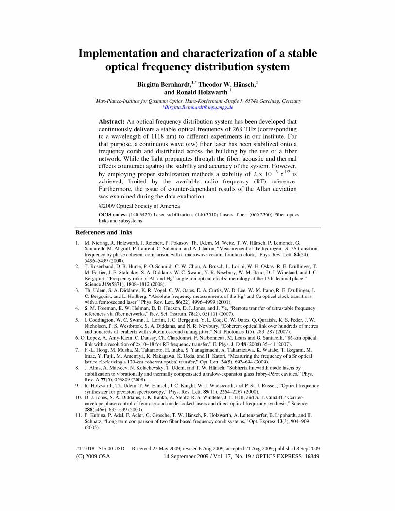
stabilization schemes, we link the optical frequency synthesizer directly to a RF reference (see

Fig. 1). The following subsections explain the particular components of the distribution

system.

Fig. 1. Basic concept of the distribution system.

2.2 The reference

Initially, the frequency comb was referenced to a commercially available Cesium clock with

high performance tube that has a specified stability of 12 1/25 10 τ− −× (Symmetricon model

5071A). In the meantime, our system could even be improved by the introduction of a

Hydrogen maser (CH1-75A, Stability: 2/113102 −−× τ ). This reference is among the most stable

RF reference sources that are commercially available and, with the comparison by GPS

signals, it is also one of the most accurate ones.

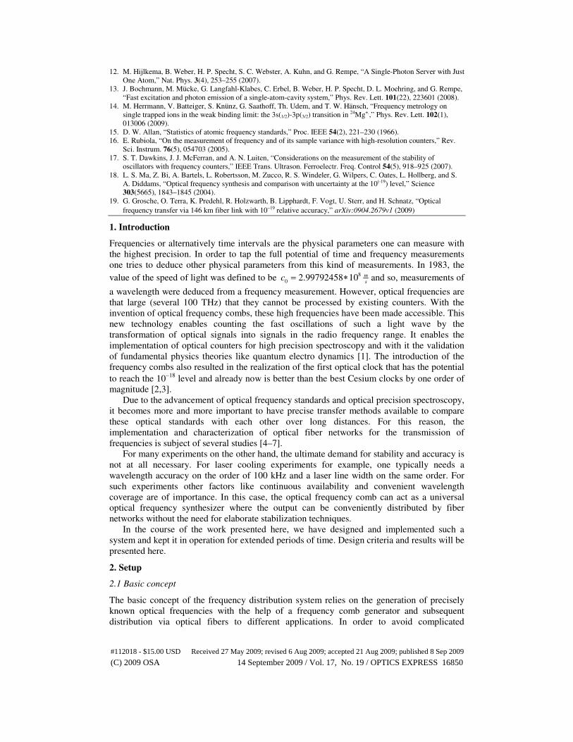
Fig. 2. Allan deviation of the references: Specifications of the Cs clock and the maser as well

as the verifying measurements of the Cs and maser stability, respectively.

The specifications of both references are shown in Fig. 2. The Allan deviation of the Cs

clock was verified by comparing it to the institute’s Hydrogen maser. Both upper curves show

that the measured data fit the manufacturer’s specification very well. The maser’s

specification (lower curve) could be checked by a long term recording of a beat note between

a diode laser stabilized to a ULE (ultra low expansion glass) high finesse cavity in vacuum

and a frequency comb referenced to the active H-maser [8]. The FP Allan deviation of this

beat note reaches a minimum of 153 10−× at 500 s. For longer times, the drift is ascribed to the

ageing process of the ULE glass and the thermal drift of the cavity.



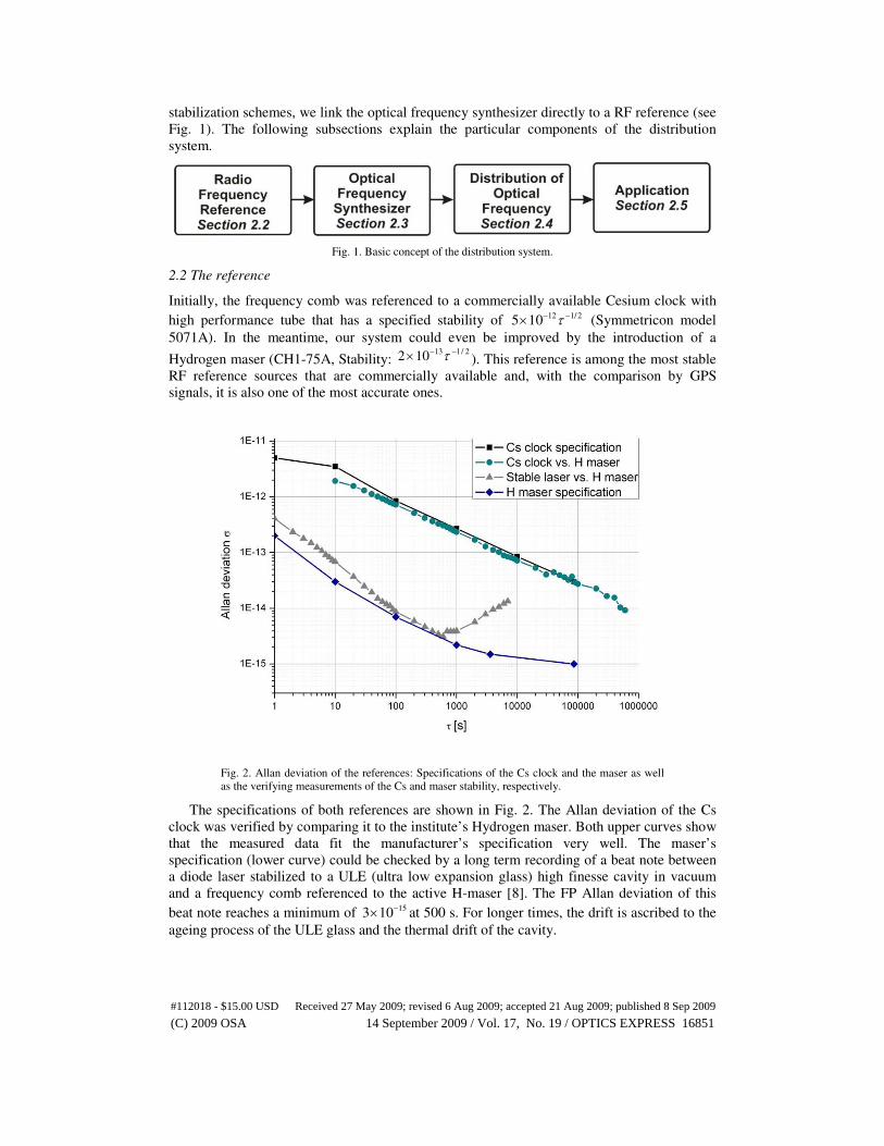
Fig. 3. Setup for the comb stability measurement, f0 and frep of the frequency combs are

stabilized via phase locked loops onto the H maser or the Cs clock.

2.3 The optical frequency synthesizer

An Erbium fiber based frequency comb generates a grid of exactly known optical reference

frequencies and serves in that way as the optical frequency synthesizer.

The pulse train emitted by a mode-locked femtosecond (fs) laser appears in the frequency

domain as a comb of equally spaced modes [9,10]. This frequency comb is completely

determined by two frequencies, f0 and frep. The offset frequency f0 is the comb's offset from

zero and is due to the phase shift between the electrical field and the pulse envelope after each

round trip in the cavity. The pulse repetition frequency frep corresponds to the spacing of the

comb modes and is linked to the cavity round trip time by frep = 1/T = vg/L, where vg is the

group velocity and L the cavity length of the laser. Because both frequencies f0 and frep are in

the radio frequency regime they can be controlled by established radio frequency techniques.

The comb is stabilized onto the Cesium clock or the Hydrogen maser as its offset and

repetition frequency are controlled via phase locked loops. To characterize the synthesizer’s

performance, a relative stability measurement was assembled without involving the fiber link.

This was realized by locking a cw laser onto an Er fiber comb and counting the beat signal

between this stabilized cw laser and a second similar Erbium fiber comb (see Fig. 3). Its

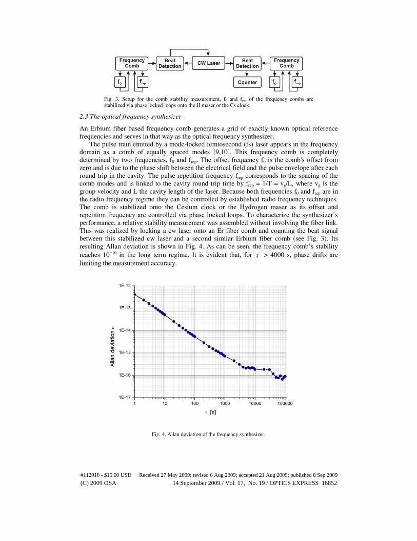
resulting Allan deviation is shown in Fig. 4. As can be seen, the frequency comb’s stability

reaches 10−16

in the long term regime. It is evident that, for τ > 4000 s, phase drifts are

limiting the measurement accuracy.

Fig. 4. Allan deviation of the frequency synthesizer.



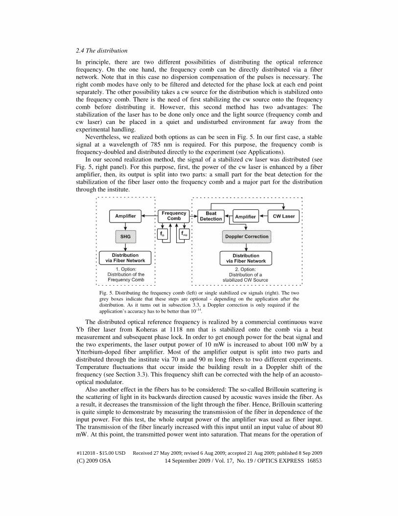
2.4 The distribution

In principle, there are two different possibilities of distributing the optical reference

frequency. On the one hand, the frequency comb can be directly distributed via a fiber

network. Note that in this case no dispersion compensation of the pulses is necessary. The

right comb modes have only to be filtered and detected for the phase lock at each end point

separately. The other possibility takes a cw source for the distribution which is stabilized onto

the frequency comb. There is the need of first stabilizing the cw source onto the frequency

comb before distributing it. However, this second method has two advantages: The

stabilization of the laser has to be done only once and the light source (frequency comb and

cw laser) can be placed in a quiet and undisturbed environment far away from the

experimental handling.

Nevertheless, we realized both options as can be seen in Fig. 5. In our first case, a stable

signal at a wavelength of 785 nm is required. For this purpose, the frequency comb is

frequency-doubled and distributed directly to the experiment (see Applications).

In our second realization method, the signal of a stabilized cw laser was distributed (see

Fig. 5, right panel). For this purpose, first, the power of the cw laser is enhanced by a fiber

amplifier, then, its output is split into two parts: a small part for the beat detection for the

stabilization of the fiber laser onto the frequency comb and a major part for the distribution

through the institute.

Fig. 5. Distributing the frequency comb (left) or single stabilized cw signals (right). The two

grey boxes indicate that these steps are optional - depending on the application after the

distribution. As it turns out in subsection 3.3, a Doppler correction is only required if the

application’s accuracy has to be better than 10−14.

The distributed optical reference frequency is realized by a commercial continuous wave

Yb fiber laser from Koheras at 1118 nm that is stabilized onto the comb via a beat

measurement and subsequent phase lock. In order to get enough power for the beat signal and

the two experiments, the laser output power of 10 mW is increased to about 100 mW by a

Ytterbium-doped fiber amplifier. Most of the amplifier output is split into two parts and

distributed through the institute via 70 m and 90 m long fibers to two different experiments.

Temperature fluctuations that occur inside the building result in a Doppler shift of the

frequency (see Section 3.3). This frequency shift can be corrected with the help of an acousto-

optical modulator.

Also another effect in the fibers has to be considered: The so-called Brillouin scattering is

the scattering of light in its backwards direction caused by acoustic waves inside the fiber. As

a result, it decreases the transmission of the light through the fiber. Hence, Brillouin scattering

is quite simple to demonstrate by measuring the transmission of the fiber in dependence of the

input power. For this test, the whole output power of the amplifier was used as fiber input.

The transmission of the fiber linearly increased with this input until an input value of about 80

mW. At this point, the transmitted power went into saturation. That means for the operation of



the system, Brillouin scattering does not occur at the required intensities and fiber lengths

since the amplifier output of 100 mW is divided into two parts for the two experiments. The

maximum power that travels through the fiber is consequently only 50 mW and lies well

beneath the crucial threshold for Brillouin scattering.

Like already mentioned, the continuous-wave fiber laser is stabilized onto the comb via an

offset frequency phase lock. For this purpose, a beat signal fbeat is observed between a cw laser

and its nearest comb mode. The optical frequency of the laser can be expressed as

0opt rep beatf mf fν = + + [11]. The two laser beams of the comb and the cw laser are overlapped

with orthogonal polarization by a polarizing beam splitter and then projected onto the same

polarization axis via an adjustable polarizer. This tuneable polarizer consists of a polarizing

beam splitter and a 2

λ -plate. A grating directly in front of the diode pre-selects several modes

of the comb in order to get a better signal to noise ratio. The output of the photo detector is

mixed with the frequency of a local oscillator and fed into a proportional-integral controller.

Its output is used to readjust the piezo controller unit inside the cw laser. The controlled beat

frequency was recorded by several counters without death time and the corresponding Allan

deviation was calculated (see section 3).

2.5 Applications

In our first case, a stable signal at a wavelength of 785 nm is needed to stabilize a cavity for

the realization of a single photon source with Rb [12]. Up to now, the cavity was stabilized

with the help of transfer cavities. The new method makes the setup easier and long-term-

stable.

As the required signal of 785 nm lies beyond the spectral range of the comb, the comb first

has to be amplified and frequency-doubled before the distribution. After the distribution, a

Diode laser (DL100 by Toptica) is phase -locked onto the comb. The single photon source

cavity is then locked onto the diode laser by a Pound-Drever-Hall-lock [13].

At the second application end, high power lasers are stabilized onto the distributed optical

standard via a beat signal detection and an offset frequency lock. While until now a complex

stabilization of the high-power lasers onto optical resonances in iodine was necessary, this is

now superseded because the frequency standard is directly distributed into the laboratories

and the lasers can be stabilized with the much easier beat detection method. Of course, there

are several other applications these newly stable high power lasers can be used for, in our case

they cool Mg+ ions that are part of our precision spectroscopy experiment [14].

The stabilization method with a frequency comb can be used for any other arbitrary

application instead of laser cooling as long as the wavelength of the laser that is to be

stabilized lies within the excessively broad comb spectrum (1000 to 2450 nm), as already

mentioned. Since the used frequency comb is a fiber based one that makes it extremely

maintainable and enables a continuous operation of the frequency distribution system so that

the experiments can be supplied with the wavelength of 1118 nm day and night.



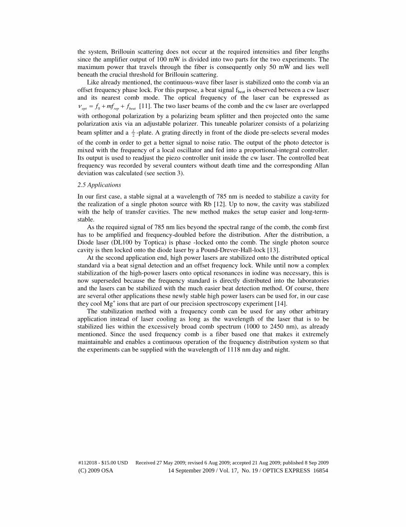
Fig. 6. (a) Beat signal between cavity stabilized laser and frequency comb (Resolution

bandwidth: 47 kHz, Signal-to-noise ratio: 22 dB), (b) locked beat signal between transfer laser

and frequency comb (Resolution bandwidth: 10 kHz, Signal-to-noise ratio: 32 dB).

3 Verification and results

3.1 Short term stability

To characterize the line width of the frequency comb locked onto the H-Maser we have

observed a beat signal with a cw laser locked onto a high finesse cavity to reduce the line

width to the Hz level. This laser is used for precision spectroscopy of Hydrogen and is

described in [8] in detail. Since this laser has Hz level line width, the main contribution to the

observed line width of 275 kHz as shown in Fig. 6(a) can be attributed to the frequency comb.

With this knowledge we have designed a relatively sloppy lock of the transfer cw laser to

the comb. The transfer laser has already a relatively narrow short term line of 45 kHz.

Therefore a sloppy lock will be enough so that the transfer laser follows the frequency comb

within its jitter. The locked beat signal is shown in Fig. 6(b), it has a line width of 90 kHz as

observed with a spectrum analyzer in 1 ms sweep time and with a resolution bandwidth of 47

kHz.

3.2 Long term stability

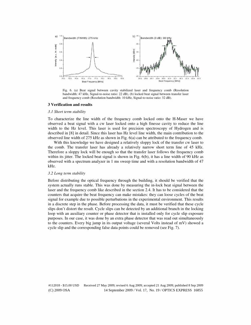
Before distributing the optical frequency through the building, it should be verified that the

system actually runs stable. This was done by measuring the in-lock beat signal between the

laser and the frequency comb like described in the section 2.4. It has to be considered that the

counters that acquire the beat frequency can make mistakes: they can loose cycles of the beat

signal for example due to possible perturbations in the experimental environment. This results

in a discrete step in the phase. Before processing the data, it must be verified that these cycle

slips don’t distort the result. Cycle slips can be detected by an additional branch in the locking

loop with an auxiliary counter or phase detector that is installed only for cycle slip exposure

purposes. In our case, it was done by an extra phase detector that was read out simultaneously

to the counters. Every big jump in its output voltage (several Volts instead of mV) showed a

cycle slip and the corresponding false data points could be removed (see Fig. 7).



Fig. 7. A change in the phase detector output voltage (a) identifies occurring cycle slips in the

frequency measurement (b).

Counter-dependant result in the Allan deviation

Out of the remaining, correct data, the Allan deviation was calculated. It is defined via the

square root of the Allan variance [15]

2 2

1

1( ) ( ) ,

2k k

y yσ τ +≡ − (1)

where the kth sample of the normalized frequency y(t), averaged over the measurement time

τ , is defined as

1

( ) .k

k

k

t

y y t dt

t

τ

τ

+

= ∫ (2)

This integral corresponds to a single (normalized) measurement of a traditional frequency

counter for a selected measurement time τ , usually called gate time. Such a traditional

frequency counter is for example the FXM counter from K&K Messtechnik that was also used

in our experiment. It takes only one value after each expired gate time. This kind of counters

is also referred to as Π -type counters. Its corresponding Allan deviation is shown by the blue

line in Fig. 8. As expected for phase locked signals, it has a time dependence of τ −1. Another

important feature of this counter that has to be emphasized is the fact that it has no dead time.

The Allan deviation as it is defined in Eq. (1) can only be derived by dead time free data.

We showed this issue by using also a second type of counter, the counter model 53131A

from Agilent (former HP). It averages the frequency value over the set gate time. These

counters are also called Λ -type counters because of their characteristic averaging method. In

contrast to the FXM counters, this special counter has a dead time where no data is acquired.

These different types of counters can affect now the final data evaluation if their different

averaging procedure is not taken into account. If one calculates the above shown Allan

deviation for the second, Λ -type counter, one gets a different, hence wrong result since the

Allan deviation is defined only for counters with a Π -type behaviour and without dead time

[16,17].

The different results out of the identical measurement setup can nicely be examined in Fig.

8. The Allan deviation extracted out of the FXM counter measurement is about two orders of

magnitude worse than the Allan deviation out of the HP measurement. This seems plausible

since the HP counter averages its acquired data during the gate time in contrast to the FXM

counter. This procedure makes the frequency appear more stable. But since the definition of

the Allan deviation only considers the phase of the starting point and the end point of every

gate time, only the FXM counter yields the true Allan deviation. Out of the averaged,



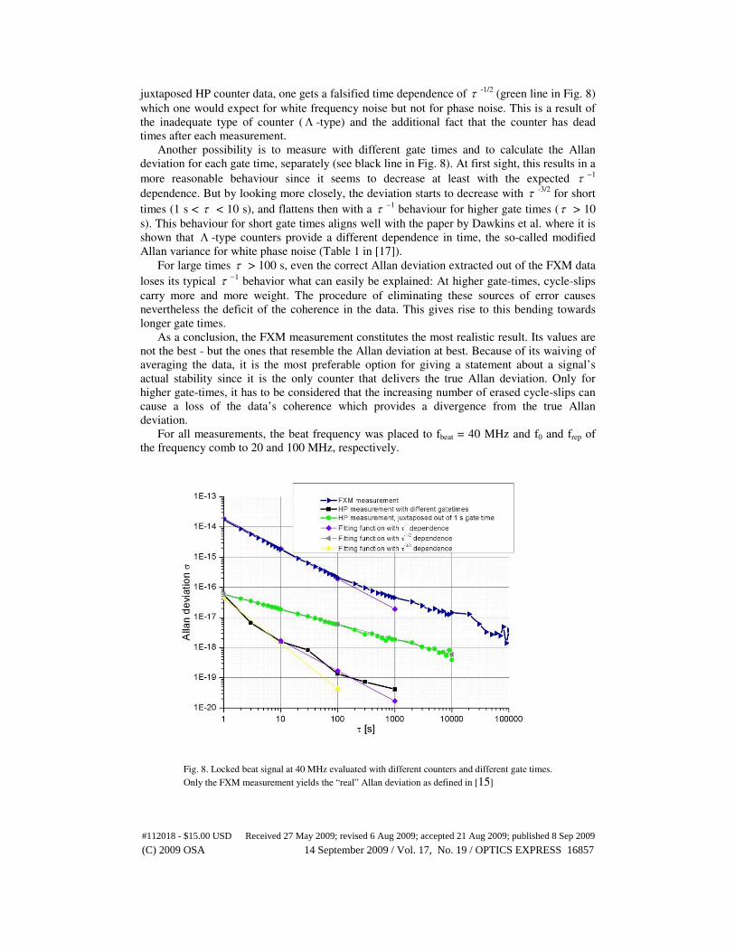
juxtaposed HP counter data, one gets a falsified time dependence of τ -1/2 (green line in Fig. 8)

which one would expect for white frequency noise but not for phase noise. This is a result of

the inadequate type of counter (Λ -type) and the additional fact that the counter has dead

times after each measurement.

Another possibility is to measure with different gate times and to calculate the Allan

deviation for each gate time, separately (see black line in Fig. 8). At first sight, this results in a

more reasonable behaviour since it seems to decrease at least with the expected τ −1

dependence. But by looking more closely, the deviation starts to decrease with τ -3/2 for short

times (1 s < τ < 10 s), and flattens then with a τ −1 behaviour for higher gate times (τ > 10

s). This behaviour for short gate times aligns well with the paper by Dawkins et al. where it is

shown that Λ -type counters provide a different dependence in time, the so-called modified

Allan variance for white phase noise (Table 1 in [17]).

For large times τ > 100 s, even the correct Allan deviation extracted out of the FXM data

loses its typical τ −1 behavior what can easily be explained: At higher gate-times, cycle-slips

carry more and more weight. The procedure of eliminating these sources of error causes

nevertheless the deficit of the coherence in the data. This gives rise to this bending towards

longer gate times.

As a conclusion, the FXM measurement constitutes the most realistic result. Its values are

not the best - but the ones that resemble the Allan deviation at best. Because of its waiving of

averaging the data, it is the most preferable option for giving a statement about a signal’s

actual stability since it is the only counter that delivers the true Allan deviation. Only for

higher gate-times, it has to be considered that the increasing number of erased cycle-slips can

cause a loss of the data’s coherence which provides a divergence from the true Allan

deviation.

For all measurements, the beat frequency was placed to fbeat = 40 MHz and f0 and frep of

the frequency comb to 20 and 100 MHz, respectively.

Fig. 8. Locked beat signal at 40 MHz evaluated with different counters and different gate times.

Only the FXM measurement yields the “real” Allan deviation as defined in [15]



3.3 Temperature effects

There are several effects that already occur in the initial laboratory that affect the stability and

the accuracy of the distributed frequency: The acoustic level in the laboratory caused by the

many devices with fans results in a spectral broadening that decreases the stability. This

spectral broadening was avoided by putting the whole setup into a sonic-isolating box. This

box, additionally, has its own fundament in order to keep off the low-frequency oscillations of

the building.

The accuracy is reduced, for example, by temperature fluctuations. These variations cause

a change of the refraction index in the fibers and an alteration of the fiber length which results

in a shift of the distributed optical frequency.

These temperature flows in the laboratory were also avoided by the box as it is also

thermally isolating. The isolating effect is that eminent as it attenuates the oscillations of the

air conditioning in the lab from about 1 °C within 10 minutes to only 0.2 °C of temperature

change within 10 hours inside the box. That corresponds to a frequency change of only 11.9

mHz for the 14 m long fiber inside the box. The frequency change is given by the

equationdn n dL T

f kLdT L dT t

∆ ∆ = + ∆

. k is the wave number. dn

dTis the ratio between refraction

index change and temperature change and 1 dL

L dT is the thermal extension coefficient of the

fiber (in our case 1.2 × 10−5

°C−1

and 11.1 × 10−7

°C−1

, respectively). That small frequency

shift means a relative accuracy of 4.44 × 10−17

.

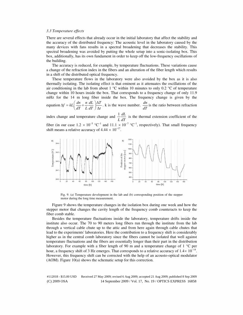
Fig. 9. (a) Temperature development in the lab and (b) corresponding position of the stepper

motor during the long time measurement.

Figure 9 shows the temperature changes in the isolation box during one week and how the

stepper motor that changes the cavity length of the frequency comb counteracts to keep the

fiber comb stable.

Besides the temperature fluctuations inside the laboratory, temperature drifts inside the

institute also occur. The 70 to 90 meters long fibers run through the institute from the lab

through a vertical cable chute up to the attic and from here again through cable chutes that

lead to the experiments' laboratories. Here the contribution to a frequency shift is considerably

higher as in the central comb laboratory since the fibers cannot be isolated that well against

temperature fluctuations and the fibers are essentially longer than their part in the distribution

laboratory. For example with a fiber length of 90 m and a temperature change of 1 °C per

hour, a frequency shift of 3 Hz emerges. That corresponds to a relative accuracy of 1.4× 10−14

.

However, this frequency shift can be corrected with the help of an acousto-optical modulator

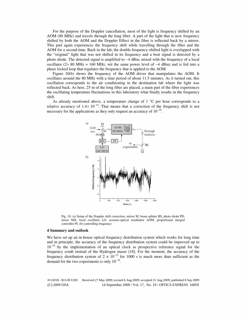
(AOM). Figure 10(a) shows the schematic setup for this correction.



For the purpose of the Doppler cancellation, most of the light is frequency shifted by an

AOM (80 MHz) and travels through the long fiber. A part of the light that is now frequency

shifted by both the AOM and the Doppler Effect in the fiber is reflected back by a mirror.

This part again experiences the frequency shift while travelling through the fiber and the

AOM for a second time. Back in the lab, the double frequency-shifted light is overlapped with

the “original” light that was not shifted in its frequency and a beat signal is detected by a

photo diode. The detected signal is amplified to −4 dBm, mixed with the frequency of a local

oscillator (2× 80 MHz = 160 MHz, wit the same power level of −4 dBm) and is fed into a

phase locked loop that regulates the frequency that is applied to the AOM.

Figure 10(b) shows the frequency of the AOM driver that manipulates the AOM. It

oscillates around the 80 MHz with a time period of about 11.5 minutes. As it turned out, this

oscillation corresponds to the air conditioning in the destination lab where the light was

reflected back. As here, 25 m of the long fiber are placed, a main part of the fiber experiences

the oscillating temperature fluctuations in this laboratory what finally results in the frequency

shift.

As already mentioned above, a temperature change of 1 °C per hour corresponds to a

relative accuracy of 1.4× 10−14

. That means that a correction of the frequency shift is not

necessary for the applications as they only request an accuracy of 10−10

.

Fig. 10. (a) Setup of the Doppler shift correction, mirror M, beam splitter BS, photo diode PD,

mixer MX, local oscillator LO, acousto-optical modulator AOM, proportional integral

controller PI; (b) controlling frequency

4 Summary and outlook

We have set up an in-house optical frequency distribution system which works for long time

and in principle, the accuracy of the frequency distribution system could be improved up to

10−18

by the implementation of an optical clock as prospective reference signal for the

frequency comb instead of the Hydrogen maser [18]. For the moment, the accuracy of the

frequency distribution system of 2 × 10−15

for 1000 s is much more than sufficient as the

demand for the two experiments is only 10−10

.



Beyond this in-house distribution network, an extensive distribution network that will link

the Max-Planck-Institut für Quantenoptik (MPQ) to the Physikalisch-Technische

Bundesanstalt (PTB) in Braunschweig is now under construction. The target of the project is

the comparison of optical frequencies at distant places. In contrast to previous methods of

modulation techniques, the frequency of a cw signal at 195 THz (i. e. 1.55 µm) will be

directly transferred via a 900 km long glass fiber link. To achieve a projected accuracy better

than 10−18

several effects like damping, stimulated Brillouin scattering, polarization mode

dispersion, amplifier noise as well as thermal and acoustic impacts have to be taken into

account [19].

This accurate transfer of optical frequencies over those unprecedented distances of

hundreds of kilometers will make precision metrology in principle accessible to every

laboratory that is within the grasp of the new far-reaching fiber distribution system.

Acknowledgements

The helpful discussions with Thomas Udem are warmly acknowledged. We also would like to

thank Arthur Matveev and Janis Alnis for providing the data record of the Cesium clock and

Hydrogen maser measurements.



Date post:	07-Oct-2016
Category:	Documents
Upload:	ronald
View:	213 times
Download:	0 times

Implementation and characterization of a stable optical frequency distribution system

Documents