IN DEGREE PROJECT ELECTRICAL ENGINEERING, SECOND CYCLE, 30 CREDITS , STOCKHOLM SWEDEN 2019 Implementation and experimental evaluation of a parameterized PMSynRM model using Matlab and Comsol Multiphysics ISRAT JAHAN KTH ROYAL INSTITUTE OF TECHNOLOGY SCHOOL OF ELECTRICAL ENGINEERING AND COMPUTER SCIENCE
Transcript
IN DEGREE PROJECT ELECTRICAL ENGINEERING,SECOND CYCLE, 30 CREDITS
, STOCKHOLM SWEDEN 2019
Implementation and experimental evaluation of a parameterized PMSynRM model using Matlab and Comsol Multiphysics
ISRAT JAHAN
KTH ROYAL INSTITUTE OF TECHNOLOGYSCHOOL OF ELECTRICAL ENGINEERING AND COMPUTER SCIENCE
i
KTH Electrical Engineering
Implementation and experimental evaluation of aparameterized PMSynRM model using Matlab and
Comsol Multiphysics
Israt Jahan
Master Thesis in Electrical Machines and Drives
KTH Royal Institute of Technology
School of Electrical Engineering and Computer Science
Division of Electric Power and Energy Systems
Supervisor:&
Examiner:
Oskar Wallmark, Associate Professor
KTH, Stockholm, Sweden, 2019
ii
Abstract
This thesis focuses on modelling of the permanent magnet synchronous reluctance
motor (PMSynRM), which has drawn considerable attention by researchers thanks to
its high efficiency and wide range of speed operation. Comparisons with measurements
from a four-pole PMSynRM with four barriers and 24 stator slots have been carried
out. In this thesis work, Matlab and Comsol Multiphysics are used to implement the
parameterized PMSynRM model.
Models of the PMSynRM in two-dimensions (2D) and three-dimensions (3D) have
been implemented. The electromotive force (back emf) at no load condition for a full-
pitch and short-pitch winding as well as the air-gap flux density distribution have been
calculated. A parametric study has been performed where the air-gap length, insulation
ratio of both d and q-axes, as well as flux barrier number have been varied and the
effect on the machine performance has been observed. The losses including eddy-
current losses in permanent magnet, stator lamination loss, and rotor lamination loss
have been calculated. The back emf and rated torque as well as developed torque with
a pure q-axis current have been compared with corresponding experimental data.
A 3D model of an axially shortened rotor has also been implemented in where a
pulsating current has been applied to estimate eddy-current losses in the permanent
magnets. The predicted losses from the 2D model and 3D model have been compared
for pulsating currents with varying frequency and magnitude.
I would like to thank Dr. Oskar Wallmark for providing his valuable time and necessary
technical information as well as other help that I needed throughout my master thesis.
I would like to thank Comsol support for their technical help during my master thesis.
I also like to thank you my family and friends to give me support to finish my master
thesis.
Israt Jahan
KTH, Sweden
May 2019
v
Table of ContentsIntroduction ............................................................................................................... 1Basic theory of SynRM and PMSynRM ............................................................ 4
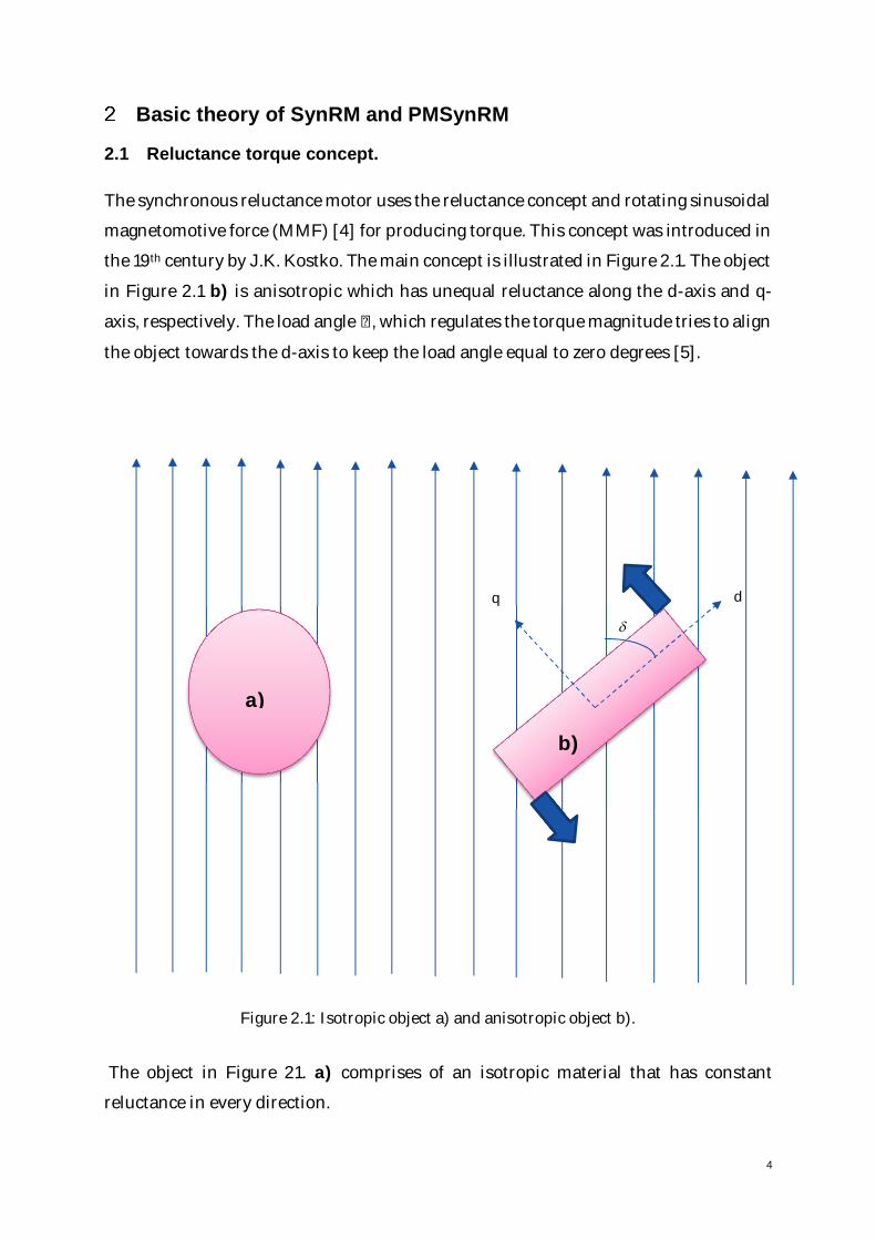
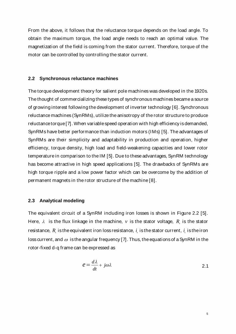
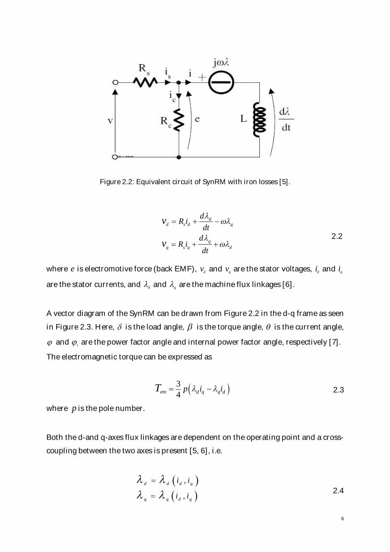
2.1 Reluctance torque concept. .................................................................................. 42.2 Synchronous reluctance machine........................................................................ 52.3 Mathematical equation ........................................................................................ 52.4 Saliency ratio ......................................................................................................... 82.5 SynRM performance............................................................................................. 82.6 Permanent magnet synchronous reluctance machine ....................................... 92.7 Construction of SynRM geometry ...................................................................... 122.8 Comparison of TLA and ALA geometry ............................................................. 152.9 IM and SynRM comparison ................................................................................ 172.10 Iron losses ............................................................................................................ 192.11 Eddy current losses in permanent magnets ..................................................... 20
2.11.1 Eddy current loss calculation per unit volume.......................................... 20Analytical design ..................................................................................................... 21
3.1 PMSynRM parameterization .............................................................................. 213.1.1 Insulation ratio ................................................................................................ 223.1.2 Flux barrier number........................................................................................ 243.1.3 Flux barrier and torque ripple ....................................................................... 243.1.4 Length of the airgap ........................................................................................ 253.1.5 Radial rib and tangential rib .......................................................................... 253.1.6 Magnet placement ........................................................................................... 273.1.7 Stator steel ....................................................................................................... 273.1.8 Permanent magnets ........................................................................................ 28
3.2 Design approach ................................................................................................. 283.2.1 Rotor barriers end angles ............................................................................... 283.2.2 MMF in d and q axes ....................................................................................... 29
3.3 Calculation of key design points ......................................................................... 31Simulation results for 2D ................................................................................... 38
4.1 Air-gap flux density ............................................................................................ 394.2 Open-circuit voltage ........................................................................................... 404.3 Open-circuit voltage in different winding ......................................................... 414.4 q-axis current ...................................................................................................... 424.5 Rated developed torque ..................................................................................... 434.6 Radial rib effect ................................................................................................... 444.7 Parametric study ................................................................................................. 45
vi
4.7.1 Change of air-gap length ................................................................................ 464.7.2 q-axis insulation ratio ..................................................................................... 464.7.3 d-axis insulation ratio ..................................................................................... 48
4.8 losses with varying frequency ............................................................................ 504.8.1 Iron losses in the stator lamination ............................................................... 504.8.2 Iron losses in the rotor lamination ................................................................. 514.8.3 Eddy-current losses in permanent magnets ................................................. 52
4.9 Losses with varying phase current .................................................................... 533D model design..................................................................................................... 54
Simulation results for 3D ................................................................................... 566.1 Eddy-current losses in permanent magnets in 3D model ............................... 56
Conclusion ............................................................................................................... 59Future work ............................................................................................................. 60Appendix A................................................................................................................ 61
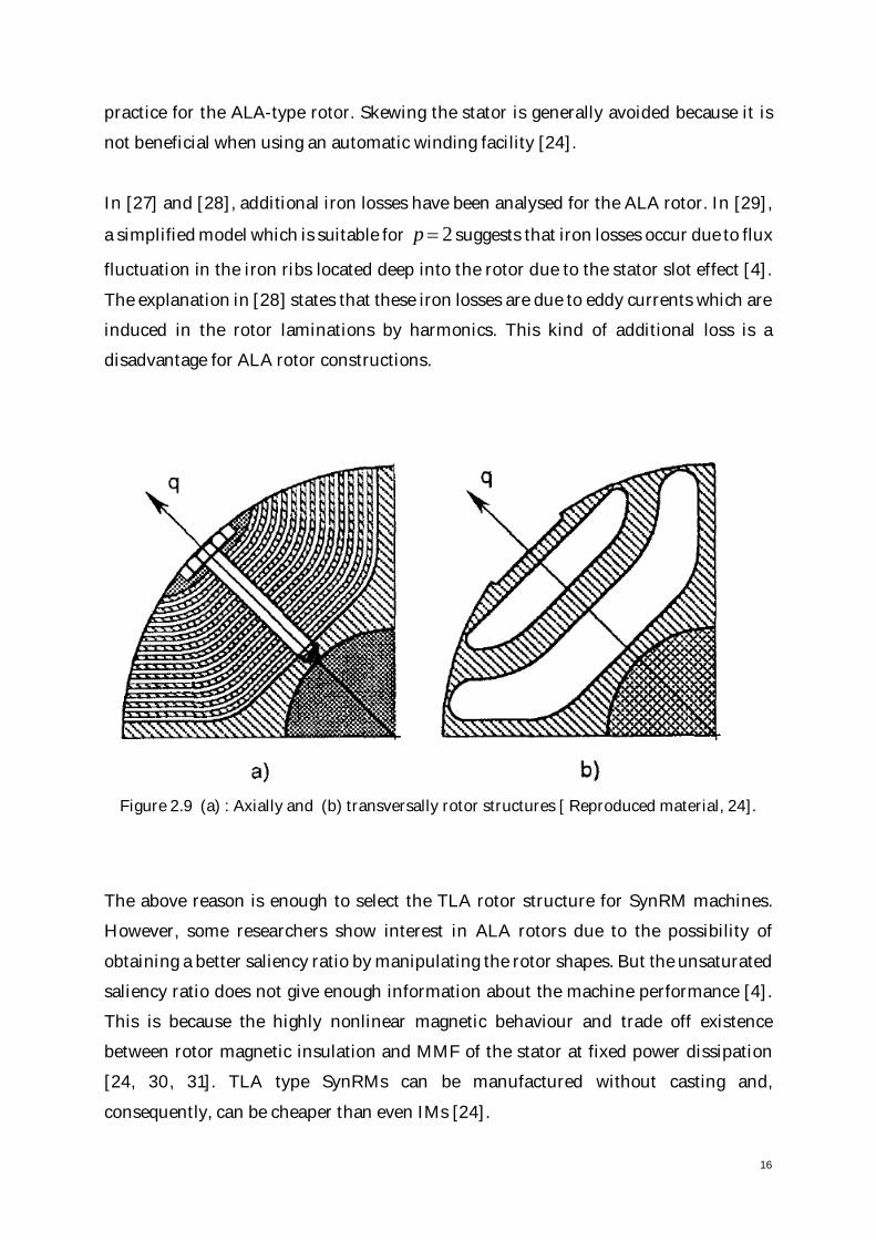
The above reason is enough to select the TLA rotor structure for SynRM machines.
However, some researchers show interest in ALA rotors due to the possibility of
obtaining a better saliency ratio by manipulating the rotor shapes. But the unsaturated
saliency ratio does not give enough information about the machine performance [4].
This is because the highly nonlinear magnetic behaviour and trade off existence
between rotor magnetic insulation and MMF of the stator at fixed power dissipation
[24, 30, 31]. TLA type SynRMs can be manufactured without casting and,
consequently, can be cheaper than even IMs [24].
17
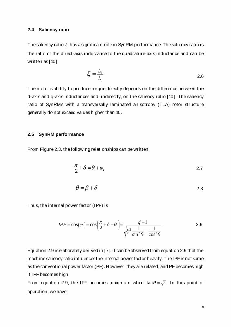
2.9 IM and SynRM comparison
The induction motor is widely used in industry because of its low cost, robustness and
capability to operate direct online without frequency converter and sophisticated
control devices. However, when speed regulation is needed to control the performance,
parameters such as torque, power factor, efficiency gain importance, and this allows to
use various types of motors [32]. The SynRM and IM machine are shown in Figure
2.10.
Production cost of SynRMs with TLA type rotors are lower compared to IMs because
of the elimination of the rotor cage. If the stator size is the same as for a corresponding
IM, just by changing the punching tools for the rotor geometry, the SynRM can be
produced in the same production line as IMs with similar sizes [32]. The TLA rotor can
also be skewed for the reduction of torque ripple which commonly is done also for IMs.
Figure 2.10: Parameters of rotor geometries for SynRM (a), and IM (b) [Reproduced
material, 33].
It is quite easy to compare performance if the stator structure and airgap diameter are
kept constant for both the SynRM and IM [23, 30, 34, 35].
Compared to IMs, the iron losses are lower in SynRMs with TLA-type rotors.
Therefore, current can be increased for the same temperature or power dissipation. It
has been demonstrated that IMs produce 20% to 40% lower toque compared to the
18
SynRMs in a similar setting. At the same stator current, the SynRM can produce 90%
to 100% of the IM torque and the total losses is about 50% lower and, consequently, a
2%-4% higher efficiency is obtained [32].
“If the stator structure can be changed then the optimum machine geometry for
maximum stall torque at constant loss power dissipation shows that the SynRM with
the ribs always has higher torque density than IM with a copper cage” [4]. Figure 2.11
shows that the inner to outer diameter ratio at the optimal airgap density (x) for
maximum stall torque is not the same for IMs and SynRMs. The value for the IM is 0.6
and for SynRM it is 0.5, as shown in Figure 2.11 [33].
Figure 2.11: Stall torque versus ratio of inner to outer diameter (4 pole machine) at the
optimum air gap flux density and overall design and optimization of Figure 2.10 geometries
[33].
The shaft and bearings in the rotor of a SynRM are cooler since there are not any losses
due to the rotor cage. The IM has a lower overload capacity compared to the SynRM
and the overload capacity of the SynRM can reach up to 3 times the nominal load [12,
T[N
m]
19
24]. Sensor-less control (meaning operation without a rotor position sensor) can be
realized for the high saliency and anisotropic rotors [32].
SynRMs have a lower power factor compared to IMs because of the cross-coupling and
larger q-axis inductance [4]. The large reactance along the q-axis is a disadvantage for
SynRMs. It depends on the rotor field distribution which is different in different areas
and is difficult to overcome. Moreover, rotor ribs flux adds to this effect [32].
The inverter sizing is directly depending on the ratio between q-axis and d-axis flux
linkage at rated condition to cope with the fixed constant power speed range [4].
However, introducing permanent magnets in the rotor can overcome this drawback
[32].
2.10 Iron losses
The prediction of iron losses in electrical machines is interesting and challenging due
to difference in production steps of the complex geometries, different material
properties, and a time varying magnetic field [36]. Three categories of iron losses arise.
Ø Eddy current loss: The electric currents that are induced in the laminations
result in resistive losses.
Ø Hysteresis loss: The flux density changes cause the loss in the structure of the
magnetic material due to movement of magnetic domain walls.
Ø Excess losses: The excess losses arise due to the interaction between the eddy
current and hysteresis loss mechanisms [37].
The hysteresis losses are proportional to the frequency while eddy current losses
are proportional to the square of the frequency. The iron losses can be written as
the sum of hysteresis and eddy current losses if a sinusoidal flux density variation
is assumed [37]
µ µ2_ s sHys HysIron loss Eddy eddyP P P k B k B
bw w= + = + 2.18
Here, _Iron lossP is the total iron loss, EddyP is total eddy current loss, H ysP is total
hysteresis loss, µB is peak flux density, sw is the angular frequency and eddyk , Hysk , b
are the co-efficients obtained by fitting the loss model from available loss data.
20
2.11 Eddy current losses in permanent magnets
Eddy current losses are generated inside the magnet of PM motors due to the
conductivity of the magnet, stator slot and MMF harmonics [38]. The eddy current
losses in the magnet is typically small compared to iron losses. However, these losses
can heat the magnets due to their poor heat dissipation through the rotor which can
result in demagnetization. This is particularly a problem for NdFeB magnet due to their
high electrical conductivity. The prototype motor considered in the thesis was built
with NdFeBs type magnets.
As the rotor and stator field rotate, a sinusoidal current is applied to the three phase
windings [38]. The magnetic flux changes due to the MMF, generated by the rotor. This
flux is dependent on the position between the stator and rotor fields [38].
However, additional MMF space harmonics of the stator field, with amplitudes
amplified by the slot openings, exist [38] and, as a result, eddy current losses are
induced in the permanent magnets.
2.11.1 Eddy current loss calculation per unit volume
The eddy current loss per unit magnet volume can be expressed as [38]
( )222
2
2
1 .12
m
m
b
mm m z
bm m
b dBk J x dxb dt
rr
-
æ ö= = ç ÷è øò 2.23
where mk is the eddy current loss per unit magnet volume, mb is magnet width, mrmagnet resistivity and B is magnetic flux density.
21
Analytical design
The rotor geometry of a SynRM is complex and it is important to define the parameters
of the geometry very well in terms of analysis. It is difficult to design the model
analytically and optimize due to the complex rotor structure and nonlinear operation
characteristics of the SynRM machine. In this section, analytical expressions will be
used to determine the geometrical parameters of the PMSynRM. Section 4 includes the
performance analysis that has been conducted with Matlab and Comsol Multiphysics.
3.1 PMSynRM parameterization
To define the rotor of the PMSynRM, the parameters of the geometry need to be
determined. Figure 3.1 shows the geometry of one pole with 3 barriers. The
parameterization conducted in this thesis are following [4] and [39].
· The barrier height is . of barrier in the direction of the q-axis and . in
the direction of the d-axis.
· The iron segment height is . of iron segment ℎ in the direction of the q-axis.
· The end point angle of barrier is . in the direction of the d-axis.
The th barrier distance is
1
. .1 1
n n
n h q k qh k
D S W-
= =
= +å å 3.1
22
Figure 3.1: Parameterization of PMSynRM.
3.1.1 Insulation ratio
It is useful to introduce a design parameter for the purpose of comparison between
different geometries, different designs and for tuning for final design called insulation
ratio that is defined as [40]
insulationw
iron
WKW
= 3.2
.
2.
.
.
.
.
.
.
.
.
.
.
.
2
23
where in s u la t io nW represents total width of flux barriers and ironW represents total
width of iron segments. In this thesis, the insulation ratio along the q-axis .w qk and
insulation ratio along the d-axis .w dk are assumed 0.6 and 0.3, respectively.
The torque production and power factor of the machine are influenced by the
insulation ratios. The reluctance in the machine is determined by these d- and q-axes
insulation ratios. It affects the flux linkage in the machine. Therefore, the saturation
level of the iron is also affected. Thus, the inductances in the machine is changed. The
inductance along the q-axis will decrease as more air is introduced in the q-axis
direction. Hence, the inductance difference is increased and, consequently, also the
saliency ratio. For the inductance difference and saliency ratio, it can be shown that
there exists an optimum in terms of .w dk and .w qk [5, 41]. The upper limit of the
insulation ratios can be described by
.s tooth
w ss
p wk p-
= 3.3
where sp is the stator slot pitch and toothw is the stator tooth width. It is desirable to
choose the value of the insulation ratio along the q-axis of the rotor to a value close to
or below the value of .w sk [4,6]. The magnitude of the flux density in the stator and
rotor is determined by the insulation ratios. Therefore, if . .w q w sk kñ , the stator teeth has
lower saturation flux than the rotor which affects the magnitude of the flux linkage at
higher current levels and, hence, affects the torque production. Thus, it was concluded
in [6] that a lower value for the q-axis insulation ratio .w qk was desirable considering
flux linkage and torque production. For the same reason, the d-axis insulation ratio
.w dk should be equal or less than the value of q-axis insulation ratio .w qk i.e., the amount
of iron along the d-axis should be higher than the amount of iron along the q-axis [4,
42].
24
3.1.2 Flux barrier number
The number of flux barriers has an influence on SynRM performance. Torque
production as well as the power factor are affected by the number of flux barriers. In
addition, the flux barrier number has great influence on the torque ripple as well as the
stator and rotor interaction. However, it is unknown how many are optimal [7]. The
selection of a suitable barrier number in the machine is complicated. A general rule
was presented in [30] to minimize the torque ripple of the SynRM machine
4r sn n= ± 3.4
where rn is the number of rotor barrier slots per pole and sn is the number of stator slots
per pole [7].
The plus or minus sign in equation 3.4 depend on the feasibility of the machine overall
structure. The performance analysis of the stator slots and number of flux barriers is
presented in [43]. It has been shown that machines with different slot and flux barrier
numbers result in different optimum performance. For example, for a machine with 48
slots and 4 poles, the maximum torque production was obtained with 4 or 6 flux
barriers. However, for the same stator, the maximum efficiency can be obtained with
4 barriers and minimum torque ripple with 6 barriers. It is shown in [11] that 4 poles
and 36 stator slots with 3 barriers result in the best performance as it results in a
maximum torque and power factor.
3.1.3 Flux barrier and torque ripple
In electrical machines, the torque ripple is an important performance index. It has been
discussed already that the stator and rotor interaction influences, machine
performance specially torque ripple. Thus, flux-barrier end positioning impacts the
machine operation.
The torque ripple is produced in SynRM machines because of reluctance variation that
occurs when the rotor barriers pass the stator slots [ 39, 44, 45, 46]. Significant amount
25
of research has been conducted to minimize this toque ripple component. Ref [44]
considers equally distributed rotor barriers and focuses on the flux barrier number
rather than rotor barrier placement and [46] focuses on the possibility of
asymmetrically placed stator slot openings to reduce the torque ripple. The article [45]
proposes to shift the rotor barriers asymmetrically between every other or several rotor
laminations [7]. However, the torque ripple optimization is not in the scope of this
project and, consequently, the investigation of the flux barrier placement is left out
from the scope.
3.1.4 Length of the airgap
It has been shown in [12] that the q-axis inductance is not dependent on the air-gap
length. However, the d-axis inductance decreases with an increase in the air-gap
length. Thus, the saliency ratio decreases. It affects the power factor as well as
production of torque. This is because the airgap is the only air the d-axis inductance
sees. Due to presence of the flux barriers, the q-axis inductance contacts with a small
fraction of total amount of air in the airgap [4]. Therefore, a lower air-gap length is
preferable to obtain a large torque of the machine. However, a large airgap results in
lower torque ripple and rotor iron losses.
3.1.5 Radial rib and tangential rib
The rotor structure of the machine is not mechanically self-sustained [4]. The flux
barriers of the rotor must be interconnected with each other. Tangential ribs are
introduced near the air gap and radial ribs are introduced along the q-axis. The q-axis
MMF will saturate these ribs during normal operation. Therefore, different flux barrier
segments are disconnected with each other from a magnetic point of view [4].
The width of the radial ribs is determined by the tolerance of the machine and expected
tangential forces from the load variation [7]. However, it is not considered in the scope
of this thesis to determine the width of the tangential ribs. Radial ribs and tangential
ribs are illustrated in Figure 3.2.
26
Figure 3.2: Radial ribs and tangential ribs in the rotor.
The size of the rotor, radial positioning of the flux barriers and maximum allowable
speed of the machine determine the need of the radial ribs (not all machines require
radial ribs) [7]. The width of the radial ribs of the machine can be calculated by dividing
the rotor into i segments and calculate the rotational force exerted on each segment
[47].
Thus, the width of the radial ribs can be expressed as
..
c ir i rib
r stk
Fw Lus
= 3.5
where rw is the width of the radial ribs, cF is the centrifugal force acting on the rotor,
rs is the tensile strength of the material, stkL is the total stack length of the rotor and
ribu is a safety factor usually in the range between 2 and 3 [47]. The centrifugal force
can be calculated as
2. ..mc i Fe iG ilam stkF R A Lr w= 3.6
27
where FeA is the area of the relevant rotor segment, GR is the center of gravity of the
rotor segment, mw is the mechanical angular frequency of the rotor, and lamr is the
mass density of the steel [47].
Introduction of radial ribs in the flux barriers structure provides an unwanted flux
path in the rotor which contributes to increase the inductance of the q-axis and,
therefore, leads to a reduction of torque production [7]. This reduction is in the
magnitude of a few percent of the nominal torque [4]. An expression of the torque
production is presented in [27] where it is found that the torque reduction is
proportional to the number of poles squared times the (assuming constant) width of
the ribs [7]. The design of the radial ribs and their influence is studied in [5].
3.1.6 Magnet placement
The placement of the magnets is quite important with regards to the performance of
the machine. [48] described that when keeping the total volume of the magnets
constant, it was more suitable in terms of torque ripple as well as torque production.
Furthermore, keeping most of the magnet volume deep within the rotor helps to
protect against demagnetisation [48] which is very important when weaker magnets
are used.
3.1.7 Stator steel
The steel lamination used for both the stator and rotor determines the iron losses of
the machine. Therefore, the steel lamination quality has an impact on machine
efficiency However, rotor iron losses in a SynRM machine is lower than the stator as
the rotor rotates synchronously with the fundamental stator flux and the rotor iron loss
is only produced by flux variations due to harmonic contents.
To reduce the iron loss in the rotor, low loss steel laminations can be used. It has been
investigated and shown in [39] that the efficiency can be increased by 9% and output
power can be increased by 8% by using low loss steel lamination in 12 kW machine
compared to more conventional (higher loss) laminations.
28
3.1.8 Permanent magnets
Magnetic behaviour is represented by the B-H curve that explains the magnetic flux
density variation with the external magnetic field [7]. Both the remanent flux density
as well as the coercivity defines the magnetic material’s characteristics. The remanent
flux density occurs when no external magnetic field is applied in the material.
Coercivity is the minimum magnetizing force that removes the remanent flux density
from the material. Available magnetic materials can be classified as hard and soft. Hard
materials have high Br and Hc value and soft magnetic materials have very low Br and
Hc values. Hard type permanent magnets are used in the prototype machine
considered in this thesis.
3.2 Design approach
After defining the geometry design parameters of the rotor are defined. The
assumptions used in this step are listed below [4]:
· Neglected saturation effects.
· Neglected stator slotting effects.
· Assumed ideal stator winding.
· Disregard MMF distribution effects.
3.2.1 Rotor barrier end angles
Rotor barrier end angles which distributed along the rotor periphery can be defined
with the constant rotor slot pitch angle, [7]
( ).
2 12 mb h
haq -
= 3.7
In this thesis, the rotor slot pitch angle is kept constant. So, the rotor slot pitch angle
can be express as
29
20.5mp
k
p
a =+
3.8
where, is rotor barrier number.
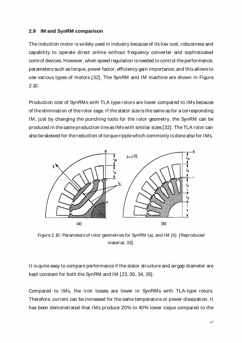
3.2.2 MMF in d and q axes
The assumed sinusoidal MMF is applied in both the d- and q-axes. Steps of constant
average MMF values as seen by the iron segment is assumed as shown in Figure 3.3
[4].
Figure 3.3: Sinusoidal MMF as function rotor periphery angle [4].
It is assumed that the rotor has k barriers. Hence, the MMF value of both the d- and
q-axes can be expressed as [7]
. 1
.
. 1 ..
. . 1 .
sin sin1 cosb i
b i
b i b id i
b i b i b if d
q
q
q qq qq q q
++
+
-= =D -ò 0,1,.......... 1i k= - 3.9a
. 1
.
. 1 ..
. . 1 .
cos cos1 sinb i
b i
b i b iq i
b i b i b if d
q
q
q qq qq q q
++
+
-= =D -ò 0,1,.......... 1i k= - 3.9b
30
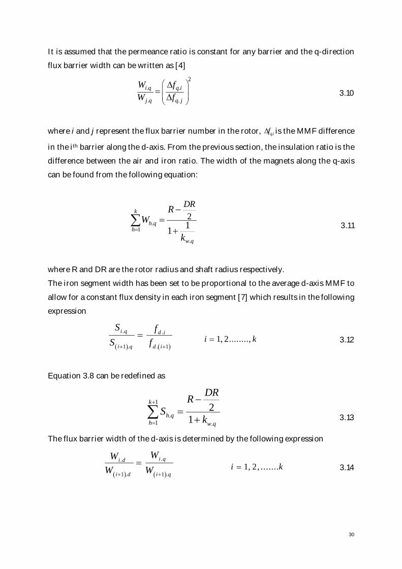
It is assumed that the permeance ratio is constant for any barrier and the q-direction
flux barrier width can be written as [4]
2. .
. .
i q q i
j q q j
W fW f
æ öç ÷ç ÷è ø
D=
D 3.10
where i and j represent the flux barrier number in the rotor, .q ifD is the MMF difference
in the ith barrier along the d-axis. From the previous section, the insulation ratio is the
difference between the air and iron ratio. The width of the magnets along the q-axis
can be found from the following equation:
.1
.
211
k
h qh
w q
DRRW
k=
-=
+å 3.11
where R and DR are the rotor radius and shaft radius respectively.
The iron segment width has been set to be proportional to the average d-axis MMF to
allow for a constant flux density in each iron segment [7] which results in the following
expression
( ) ( )
. .
1 . . 1
i q d i
i q d i
S fS f+ +
= 1, 2........,i k= 3.12
Equation 3.8 can be redefined as
1
.1 .
21
k
h qh w q
DRRS
k
+
=
-=
+å 3.13
The flux barrier width of the d-axis is determined by the following expression
( ) ( )
..
1 . 1 .
i qi d
i d i q
WWW W+ +
= 1, 2, .......i k= 3.14
31
3.3 Calculation of key design points
Figure 3.4 shows the key design points for understanding the PMSynRM rotor
geometry.
Figure 3.4: Key design points for a PMSynRM with a single flux barrier.
First, equations for the rectangular shape has been generated in Figure 3.5, where p
is the pole pair, 1S is the width of the iron segment, 1L is half of the height of the magnet,
lqW is the width of the magnet,2
DR is the shaft radius, R is the rotor radius, and TR
is the width of the tangential rib.
32
Figure 3.5: Key design points for magnet shape.
Points A1 and A2 are the intersection points of the flux barriers with q-axis:
Point A1
1 1
1 1
cos2 2
sin2 2
A
A
DR Sp
DRy Sp
x p
p
æ öæ ö= + ç ÷ç ÷è ø è ø
æ öæ ö= + ç ÷ç ÷è ø è ø
3.15
33
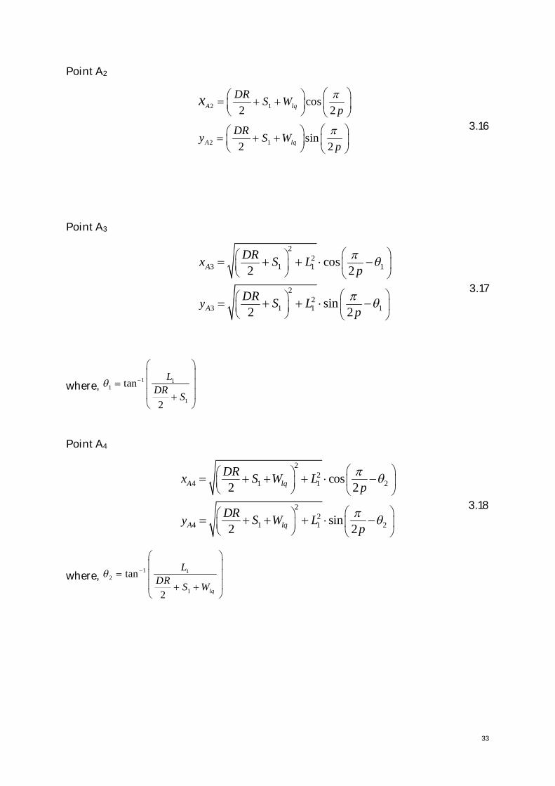
Point A2
2 1
2 1
cos2 2
sin2 2
A lq
A lq
DR S Wp
DRy S Wp
x p
p
æ öæ ö= + + ç ÷ç ÷è ø è ø
æ öæ ö= + + ç ÷ç ÷è ø è ø
3.16
Point A3
22
3 1 1 1
22
3 1 1 1
cos2 2
sin2 2
A
Ay
DRx S Lp
DR S Lp
p q
p q
æ öæ öç ÷ç ÷
è ø è ø
æ öæ öç ÷ç ÷
è ø è ø
= + + × -
= + + × - 3.17
where,1 1
1
1
tan
2
LDR S
q -
æ öç ÷
= ç ÷ç ÷+è ø
Point A4
22
4 1 1 2
22
4 1 1 2
cos2 2
sin2 2
A lq
A lqy
DRx S W Lp
DR S W Lp
p q
p q
æ öæ öç ÷ç ÷
è ø è ø
æ öæ öç ÷ç ÷
è ø è ø
= + + + × -
= + + + × - 3.18
where,1 1
2
1
tan
2 lq
LDR S W
q -
æ öç ÷
= ç ÷ç ÷+ +è ø
34
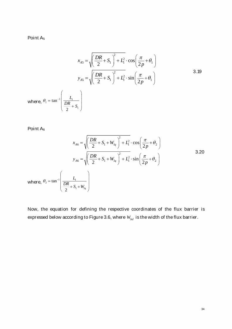
Point A5
22
5 1 1 1
22
5 1 1 1
cos2 2
sin2 2
A
Ay
DRx S Lp
DR S Lp
p q
p q
æ öæ öç ÷ç ÷
è ø è ø
æ öæ ö +ç ÷ç ÷è ø è ø
= + + × +
= + + × 3.19
where,1 1
1
1
tan
2
LDR S
q -
æ öç ÷
= ç ÷ç ÷+è ø
Point A6
22
6 1 1 2
22
6 1 1 2
cos2 2
sin2 2
A lq
A lqy
DRx S W Lp
DR S W Lp
p q
p q
æ öæ öç ÷ç ÷
è ø è ø
æ öæ ö +ç ÷ç ÷è ø è ø
= + + + × +
= + + + × 3.20
where,1 1
2
1
tan
2 lq
LDR S W
q -
æ öç ÷
= ç ÷ç ÷+ +è ø
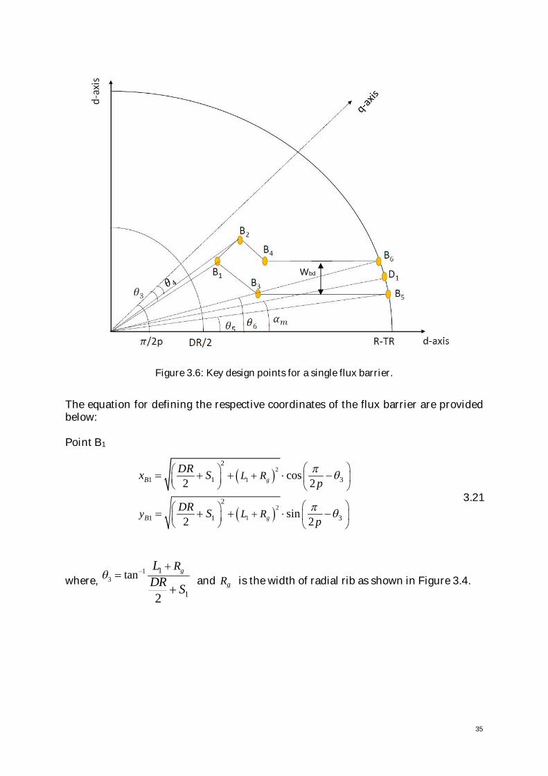
Now, the equation for defining the respective coordinates of the flux barrier is
expressed below according to Figure 3.6, where bdW is the width of the flux barrier.
35
Figure 3.6: Key design points for a single flux barrier.
The equation for defining the respective coordinates of the flux barrier are providedbelow:
Point B1
( )
( )
2
1
2
1
2
1 1 3
2
1 1 3
cos2 2
sin2 2
g
g
B
B
L R
y L R
DRx Sp
DR Sp
p q
p q
æ öæ ö + ç ÷ç ÷è ø è ø
æ öæ ö + ç ÷ç ÷è ø è ø
= + + × -
= + + × - 3.21
where,1
31
1
tan
2
gRLDR S
q - +=
+ and gR is the width of radial rib as shown in Figure 3.4.
Wbd
36
Point B2
( )
( )
2
1
2
1
2
2 1 4
2
2 1 4
cos2 2
sin2 2
g
g
B lq
B lq
L R
y L R
DRx S Wp
DR S Wp
p q
p q
æ öæ ö + ç ÷ç ÷è ø è ø
æ öæ ö + ç ÷ç ÷è ø è ø
= + + + × -
= + + + × - 3.22
where, 14
1
1
tan
2
g
lq
RLDR S W
q - +=
+ +
Points B5 and B6 represent the intersection points of the flux barrier with the rotor
outer periphery:
Point B5
( )( )
5 5
5 5
cossin
B
B
R TRy R TRx q
q
= -
= - 3.23
where,1
51 2sin
bdD
Wy
R TRq -
æ ö-ç ÷= ç ÷
-ç ÷ç ÷è ø
Point B6
( )( ) 6
6 6
6
cossin
B
B
R TRy R TRx q
q
= -
= - 3.24
where,1
61 2sin
bdD
Wy
R TRq -
æ ö+ç ÷= ç ÷
-ç ÷ç ÷è ø
37
Points D1 represents the mid endpoints of the flux barriers:
Point D1
( )( )
1
1
cossin m
mD
D
R TRy R TRx a
a
= -
= - 3.25
Points B3 and B4 are the intersection points of the different lines of the flux barriers:
Point B3
5 51
3
53
1
tan2
1
tan2
B BB
B
BB
y y x
p
py
x
y
p
p
æ öç ÷è ø
æ öç ÷è ø
- -
=-
=
3.26
Point B4
6 2 6
4
4 6
1
tan2
1
tan2
B B B
B
B B
y y x
p
py
x
y
p
p
æ öç ÷è ø
æ öç ÷è ø
- -
=-
=
3.27
38
Simulation results in 2D
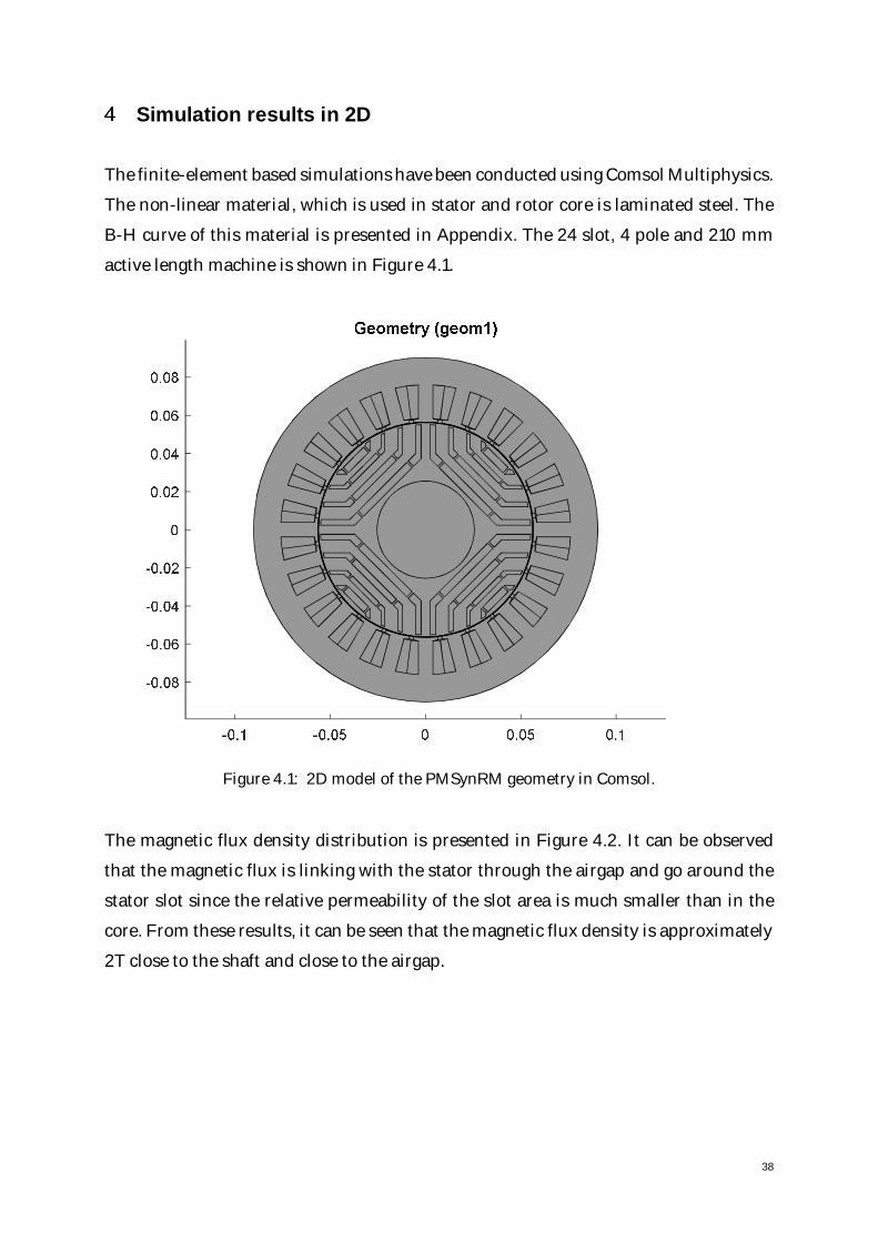
The finite-element based simulations have been conducted using Comsol Multiphysics.
The non-linear material, which is used in stator and rotor core is laminated steel. The
B-H curve of this material is presented in Appendix. The 24 slot, 4 pole and 210 mm
active length machine is shown in Figure 4.1.
Figure 4.1: 2D model of the PMSynRM geometry in Comsol.
The magnetic flux density distribution is presented in Figure 4.2. It can be observed
that the magnetic flux is linking with the stator through the airgap and go around the
stator slot since the relative permeability of the slot area is much smaller than in the
core. From these results, it can be seen that the magnetic flux density is approximately
2T close to the shaft and close to the airgap.
39
Figure 4.2: Magnetic flux density distribution.
4.1 Air-gap flux density
For no-load condition, the radial component of the air-gap flux density is presented in
Figure 4.3. it can be observed that the simulation results obtained from FEM are
different than the results obtained from the analytical calculations due to magnetic
saturation.
40
Figure 4.3: Air-gap flux density as function of electrical angle at no load.
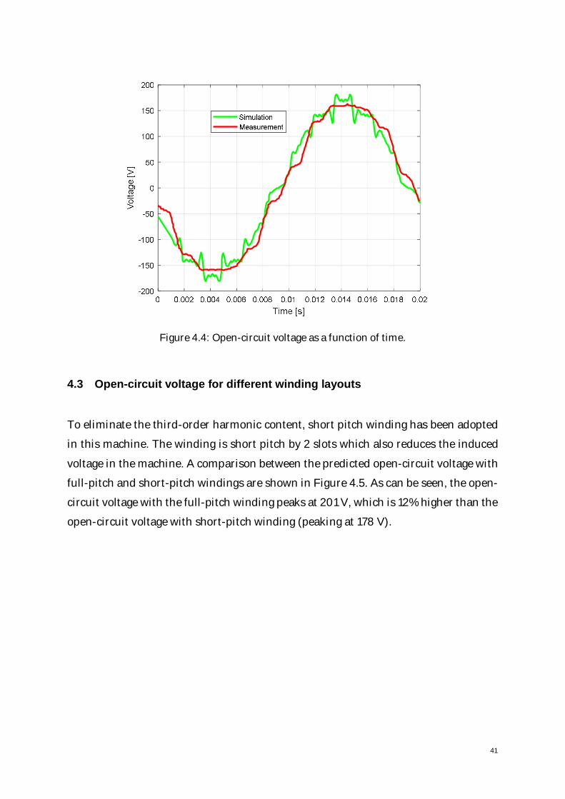
4.2 Open-circuit voltage
With a rotational speed of the rotor of 1500 rpm, according to Faraday’s law, a voltage
will be induced in the coils. The induced open- circuit voltage in a coil is presented in
Figure 4.4 and compared with measured data (the measured data was obtained from
[40]). It can be observed that the agreement between the measured and predicted
voltage waveforms are agreeing relatively well. However, further studies are required
in order to improve this agreement.
41
Figure 4.4: Open-circuit voltage as a function of time.
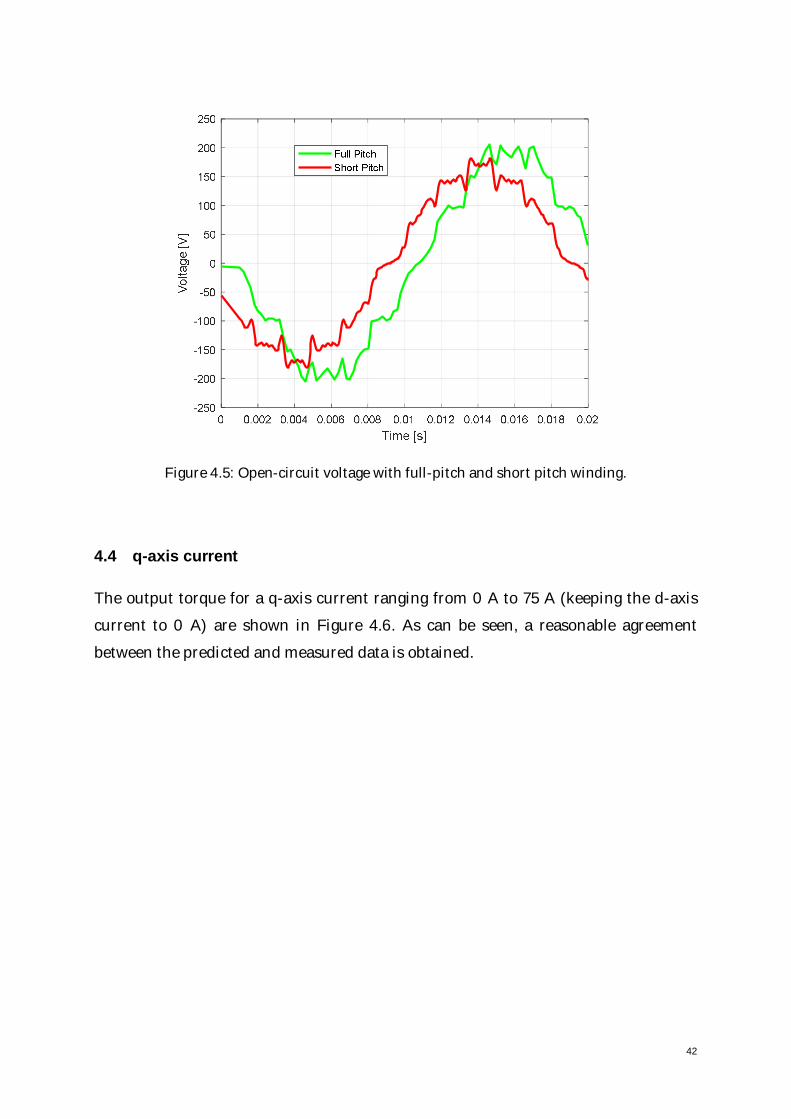
4.3 Open-circuit voltage for different winding layouts
To eliminate the third-order harmonic content, short pitch winding has been adopted
in this machine. The winding is short pitch by 2 slots which also reduces the induced
voltage in the machine. A comparison between the predicted open-circuit voltage with
full-pitch and short-pitch windings are shown in Figure 4.5. As can be seen, the open-
circuit voltage with the full-pitch winding peaks at 201 V, which is 12% higher than the
open-circuit voltage with short-pitch winding (peaking at 178 V).
42
Figure 4.5: Open-circuit voltage with full-pitch and short pitch winding.
4.4 q-axis current
The output torque for a q-axis current ranging from 0 A to 75 A (keeping the d-axis
current to 0 A) are shown in Figure 4.6. As can be seen, a reasonable agreement
between the predicted and measured data is obtained.
43
Figure 4.6: Output torque as a funtion of q-axis current.
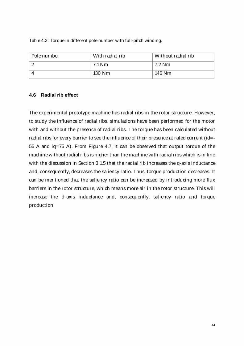
4.5 Rated developed torque
Simulated average torque values for the machine with short and full-pitch windings
are presented in Table 4.1 and 4.2, respectively, for the geometry with and without the
introduction of radial ribs. It can be pointed out that the rated output torque for the
short-pitch winding is 117 Nm and the rated torque for the full-pitch is 130 Nm with
rated current (id=-55 A and iq=75 A) for four pole machines. For a corresponding two-
pole machine, the rated output torque is small, as the two-pole machine does not yield
the required reluctance to produce torque.
Table 4.1: Torque in different pole number with short-pitch winding.
Pole number With radial rib Without radial rib
2 6.4 Nm 6.6 Nm
4 117 Nm 125 Nm
44
Table 4.2: Torque in different pole number with full-pitch winding.
Pole number With radial rib Without radial rib
2 7.1 Nm 7.2 Nm
4 130 Nm 146 Nm
4.6 Radial rib effect
The experimental prototype machine has radial ribs in the rotor structure. However,
to study the influence of radial ribs, simulations have been performed for the motor
with and without the presence of radial ribs. The torque has been calculated without
radial ribs for every barrier to see the influence of their presence at rated current (id=-
55 A and iq=75 A). From Figure 4.7, it can be observed that output torque of the
machine without radial ribs is higher than the machine with radial ribs which is in line
with the discussion in Section 3.1.5 that the radial rib increases the q-axis inductance
and, consequently, decreases the saliency ratio. Thus, torque production decreases. It
can be mentioned that the saliency ratio can be increased by introducing more flux
barriers in the rotor structure, which means more air in the rotor structure. This will
increase the d-axis inductance and, consequently, saliency ratio and torque
production.
45
Figure 4.7: Output torque with and without radial ribs as a function of barrier number.
4.7 Parametric study
A parametric study has been conducted with varying airgap, d-axis and q-axis
insulation ratio with full-pitch and short-pitch winding, as well as three and four
barriers with and without radial ribs to observe the torque behavior. Table 4.3 shows
values valid for the experimental prototype machine.
Table 4.3: Base input for parametric study.
Base input Description Value
g Air-gap Length 0.35 [mm]
kwd d-axis insulation ratio 0.3
kwq q-axis insulation ratio 0.6
Wt.i Tangential ribs 1 [mm]
Wr.i Radial ribs 1 [mm]
46
4.7.1 Change of air-gap length
The air-gap length of the prototype machine is 0.35 mm. The air-gap length has been
varied from 0.2mm to 0.85mm to observe the output torque with three and four
barriers at rated current. It can be observed from Figure 4.8 that the output torque
decreases with an increase in the air-gap length. It has been mentioned in Section 3.1.4
that the air-gap length affects the d-axis inductance. The d-axis inductance decreases
as air-gap length increases and, consequently, the torque production is decreased.
Figure 4.8: Output torque as a function of the air-gap length.
4.7.2 q-axis insulation ratio
Figure 4.9 shows the cross-sectional area of the rotor for the q-axis insulation ratios
corresponding to 0.5 and 0.8 using three flux barriers. The prototype machine has been
designed for the q-axis insulation ratio of 0.6. To justify the designed value, in this
thesis, the q-axis insulation ratio has been varied from 0.5 to 0.8 for both three and
four barriers and the output torque has been calculated. The output torque of the
machine with three and four barriers in the rotor is presented in Figure 4.10 as a
function of q-axis insulation ratio. It can be observed from the presented results that
47
the output torque increases as the q-axis insulation ratio increases and reaches an
optimal value at 0.6. This means that the d-axis inductance increases with an increase
in the amount of air in the rotor structure but at a certain value, this inductance starts
to decrease. It can also be observed that the four-barrier rotor structure has a higher
torque capability than the three-barrier rotor structure.
Figure 4.9: kwq=0.5 (left) and kwq=0.8 (right)
48
Figure 4.10: Variation of output torque as a function of the q-axis insulation ratio.
4.7.3 d-axis insulation ratio
The rotor geometries with three flux barriers are presented in Figure 4.11 for d-axis
insulation ratios of 0.2 and 0.5, respectively. To study the influence on output torque,
the ratio has been varied from 0.2 to 0.5 for three and four barriers. The calculated
output torque of the machine for the three and four flux barriers have been presented
in Figure 4.12 as function of the d-axis insulation ratio. It can be observed from the
simulation results that the trend of torque variation with the d-axis insulation ratio
variation is quite similar for both the three and four barrier rotor structures and both
have their optimal value at 0.3. However, the four-flux barrier rotor structure is
capable to producing more torque than the three-flux barrier rotor structure.
Torq
ue[N
m]
49
Figure 4.11: kwd=0.2 (left) and kwd=0.5 (right)
Figure 4.12: Variation of output torque as a function of the d-axis insulation ratio.
Torq
ue[N
m]
50
4.8 losses with varying frequency
4.8.1 Iron losses in the stator lamination
The losses in the stator lamination have been calculated with and without radial ribs
for both the full-pitch and short-pitch winding with injecting sinusoidal current in d-
axis ( 30sindi tw= ). The calculated iron losses in the stator lamination are presented in
Figure 4.13 as a function of the operating frequency of the machine. It can be observed
that the iron losses in the stator lamination is increasing as frequency increases.
Introduction of radial ribs in the flux barriers structure provide an unwanted flux path
in the rotor which contributes to increase the flux fluctuation in the machine and,
consequently, increase the iron losses. Thus, the machine with the radial rib rotor
structure for full-pitch winding results in higher losses. The winding has been chorded
by 2/3 and this practically eliminate the third harmonic from the harmonic’s spectrum.
Thus, the full-pitch winding arrangement shows the higher iron losses in the stator
lamination than the short pitch winding.
Figure 4.13: Iron losses in the stator lamination as a function of operating frequency for bothshort and full-pitch winding as well as with and without radial rib.
Iron
loss
esin
the
stat
orla
min
atio
n[W
]
51
4.8.2 Iron losses in the rotor lamination
Similar to the stator lamination, the losses in the rotor laminations have been
calculated with and without radial ribs for both the both full-pitch and short-pitch
winding. Losses in the rotor lamination are presented in Figure 4.14 as a function of
the operating frequency of the machine. It can be observed from the simulation results
that the losses in the rotor laminations also increase with increasing the fundamental
operating frequency of the machine. As can be seen, the iron losses in the rotor
laminations is somewhat higher for the full-pitch winding compared to the short-pitch
winding.
Figure 4.14: Iron losses in the rotor lamination as a function of operating frequency for bothshort and full-pitch winding as well as with and without radial rib.
Iron
loss
esin
the
roto
rlam
inat
ion
[W]
52
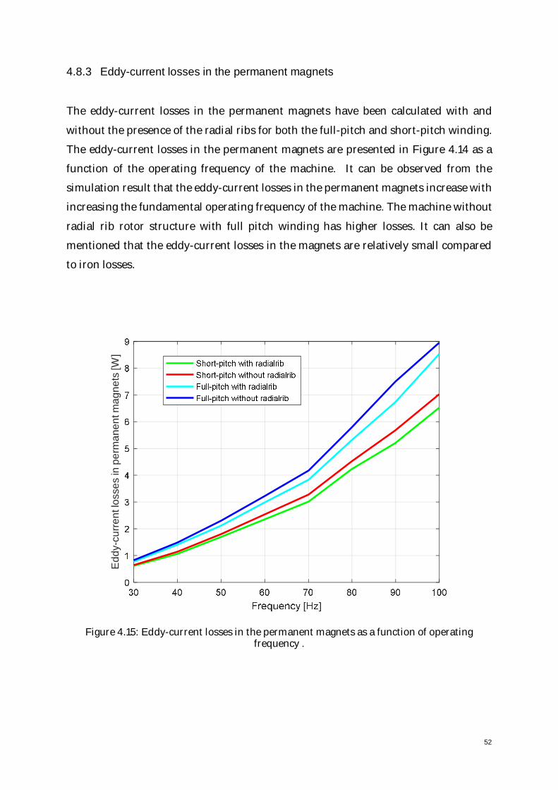
4.8.3 Eddy-current losses in the permanent magnets
The eddy-current losses in the permanent magnets have been calculated with and
without the presence of the radial ribs for both the full-pitch and short-pitch winding.
The eddy-current losses in the permanent magnets are presented in Figure 4.14 as a
function of the operating frequency of the machine. It can be observed from the
simulation result that the eddy-current losses in the permanent magnets increase with
increasing the fundamental operating frequency of the machine. The machine without
radial rib rotor structure with full pitch winding has higher losses. It can also be
mentioned that the eddy-current losses in the magnets are relatively small compared
to iron losses.
Figure 4.15: Eddy-current losses in the permanent magnets as a function of operatingfrequency .
Eddy
-cur
rent
loss
esin
perm
anen
tmag
nets
[W]
53
4.9 Losses with varying phase current
The losses of the stator and rotor laminations as well as the permanent magnets have
been calculated for the machine with short-pitch winding and radial rib rotor structure.
The d- and q-axes current have been increased linearly and losses have been calculated.
The losses are presented in Figure 4.16 as a function of phase current (rms). It can be
observed from the presented results that the losses are increasing as the phase current
is increased. Also, it can be said that the losses in the stator laminations are higher than
the losses in the rotor laminations and permanent magnets.
Figure 4.16: Losses in the stator and rotor lamination and permanent magnets as a functionof phase current (rms).
Loss
es[W
]
54
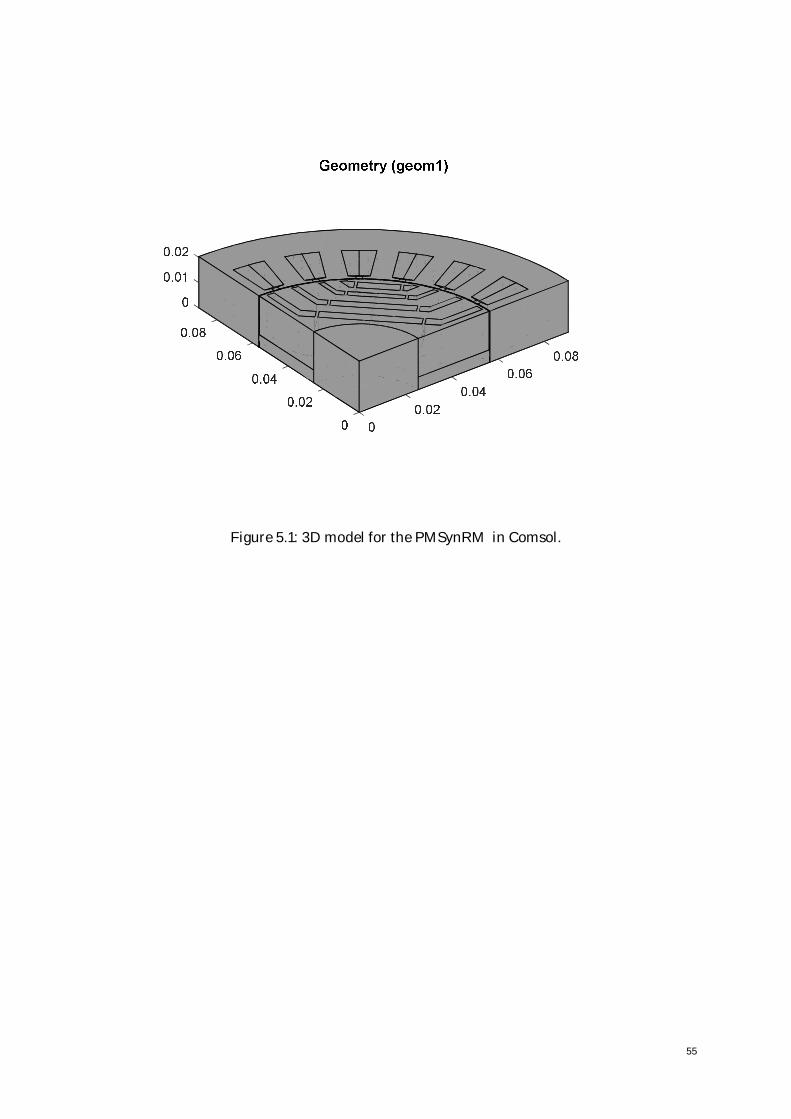
3D model design
A 3D model has been created by extruding the 2D model.
5.1 Stator modeling
In the 3D model, the active length of the rotor has been considered shorter than the
stator. The active length of the rotor is 30 mm long and for the stator, it is 40 mm.
However, to reduce the simulation time, only half of the axial length of the stator and
rotor has been simulated and only one fourth of the total cross-sectional area is
considered. Thus, the 3D model stator length is 20 mm with 6 stator slots.
5.2 Rotor modeling
By considering symmetry of the geometry, one pole of the rotor has been modelled.
The axial length of the modelled rotor lamination is 15 mm. However, the shaft has
been modelled for 20 mm axial length. Since the shaft material has a negligible
influence on the torque production, it has been modelled as air. The permanent
magnets are segmented and each of the segmented magnet is 10 mm. So, in the 30 mm
rotor, there are three permanent magnets with very small airgap between each magnet.
In this design, one 10 mm magnet and one 5 mm magnet has been designed with 0.005
mm airgap between them. The airgap functions as electrical insulation, so no eddy-
currents penetrate the gap. This makes the eddy-current loop shorter and the eddy-
current losses in permanent magnets are reduced compared to losses calculated by
using 2D analysis. Figure 5.1 presents the modelled 3D geometry of the PMSynRM
machine.
55
Figure 5.1: 3D model for the PMSynRM in Comsol.
56
Simulation results in 3D
The magnetic flux density distribution is presented in Figure 6.1 with non-linear
laminated steel. It can be observed that the magnetic flux density distribution in 3D
models is similar to the flux distribution in 2D model.
Figure 6.1: Magnetic flux density distribution in 3D model with non-linear laminated steel.
6.1 Eddy-current losses in permanent magnets in 3D model
Eddy-current losses have been calculated by using both the 2D and 3D finite element
analysis (FEA) with injecting sinusoidal current in d-axis ( 30sindi tw= ). The current in
the q-axis current remain zero. The calculated eddy-current losses using the 2D and
3D models are presented in Figure 6.2 as a function of the operating frequency of the
machine. It can be observed that the calculated losses are increased with increasing
the fundamental operating frequency of the machine for both the 2D and 3D FEA.
However, there is significant difference between the calculated eddy-current losses by
using 2D and 3D FEA. In 2D, the magnet has been considered as 1 piece with 3o mm
long and axial segmentation has been neglected. However, in 3D, the magnet is
segmented, and each segment is 10 mm long. Axial segmentation intersect the bigger
eddy current loop and reduce the total amount of eddy-current loss. In the 3D model,
57
segmentation has been modelled by using the electric insulation between two magnet
segments. The 3D eddy-current distribution in the permanent magnets is presented in
Figure 6.3.
Figure 6.2: Comparison of eddy-current losses in permanent magnets in 2D and 3D model as
a function of the operating frequency.
Eddy
-cur
rent
loss
esin
perm
anen
tmag
nets
[W]
58
Figure 6.3: Eddy-currents distribution in permanent magnets by using 3D FEA.
59
Conclusion
In this thesis, parameterized two-dimensional (2D) and three-dimensional (3D) finite
element models of permanent-magnet synchronous reluctance machine (PMSynRM)
machine have been implemented using Matlab and Comsol Multiphysics.
Basic theory and phasor diagram of the synchronous reluctance machine (SynRM),
PMSynRM, different type of rotor geometries as well as a comparison with IMs have
been discussed. The important parameters, such as number and widths of flux barriers,
iron segments, rotors point end angles, radial and tangential ribs are described and are
shown to have a significant impact on machine performance.
A parametric study has been conducted by varying design parameters to study the
machine performance using the developed finite element model. It has been found that
the number and width of the flux barriers in the rotor affected the torque of the
machine significantly. Finite element analysis (FEA) and comparison with
measurements from a four-pole PMSynRM with four barriers and 24 stator slots have
also been carried out. It was observed from the simulation results that both the d-and
q-axis insulation ratio and number of flux barriers have been designed optimally for
the prototype machine.
The air-gap flux density distribution and the open-circuit voltage of the machine for a
full-pitch and short-pitch winding have been calculated. The eddy-current losses in
permanent magnets, iron losses in the stator and rotor lamination have also been
calculated. The output torque has been calculated for a 2- and 4-pole machine with
and without radial rib with full-pitch and short-pitch distributed winding.
The 3D model of an axially shortened rotor has been implemented and losses in the
permanent magnets have been calculated by applying a pulsating current and varying
the supply frequency and magnitude. The predicted losses from 2D FEA and 3D FEA
have been compared. Due to the segmented magnet structure in 3D FEA, the eddy-
current losses are significantly lower than the losses obtained from 2D FEA.
60
Future work
The following ideas for future work are suggested:
1. A more in-depth parametric study to optimize the machine performance can be
carried out.
2. Thermal analysis is one of the keys to compare torque capability of the machine
as cooling capacity can be limiting factor to design motor with higher torque.
3. Conduct accoustic analysis to study the noise and vibration
4. Investigate flux fluctuation in the rotor and observe its effect on both torque
ripple as well as iron losses.
5. Investigate torque ripple and develop an effective procedure to reduce the
torque ripple.
6. Select and implemented an effective control system and perform field-
weakening operation.
61
Appendix A
A.1 B-H curveB-H curve of the laminated steel material has shown in Figure 9.1.
Figure 9.1: B-H curve of the laminated steel material [49].
62
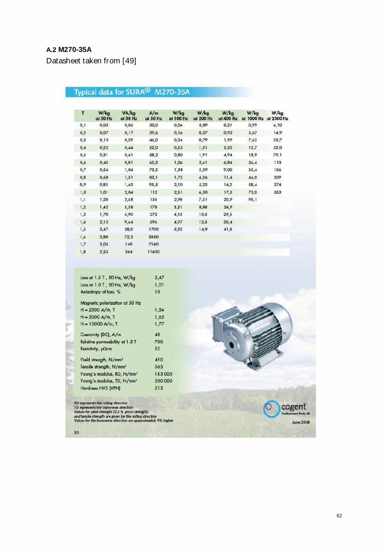
A.2 M270-35ADatasheet taken from [49]
63
64
Reference
[1] M. Sanada et al. “Torque Ripple Improvement for Synchronous Reluctance Motor
Using an Asymmetric Flux Barrier Arrangement”, IEEE Transactions on
Industry Applications, Vol. 40, No. 4, July/August 2004.
[2] V.S. Nagarazan et al. ” Effect of Geometrical Parameters on Optimal Design of
Synchronous Reluctance Motor”, Journal of Magnetics, 21(4), 544-553 (2016)
[3] S.Nageth et al “ Thermal Analysis of a PMaSRM Using Partial FEA and Lumped
Parameter Modeling”, IEEE Transactions on Energy Conversion, Vol. 27, No. 2,