44
WORKING PAPER NO. 39 JUNE 2010 Wildlife Picture Index: Implementation Manual Version 1.0 Tim O’Brien

w o r k i n g p a p e r n o . 3 9 J u n e 2 0 1 0
Wildlife Picture Index: Implementation Manual Version 1.0
Tim O’Brien


WILDLIFE PICTURE INDEX:IMPlementation Manual Version 1.0
WCS Working PaPer no. 39June 2010
Tim O'BrienSenior Conservation Scientist, Conservation SupportWildlife Conservation Society2300 Southern BoulevardBronx, NY 10460254 0 62 [email protected]
By Tim o'Brien

ii Wildlife Conservation Society | WORKING PAPER NO. 39
WCS Working Papers: ISSN 1530-4426Online posting: ISSN 1534-7389
Copies of WCS Working Papers are available from:Wildlife Conservation SocietyGlobal Conservation2300 Southern BoulevardBronx, NY 10460-1099 USA
Suggested citation:O’Brien, Tim. Wildlife Picture Index: Implementation Manual Version 1.0. WCS Working Papers No. 39, June 2010.
Cover image: Aardvark (Orycteropus afer) camera trap photograph © WCS
Copyright:The contents of this paper are the sole property of the author, and cannot be reproduced without permission of the author.
The Wildlife Conservation Society saves wildlife and wild places world-wide. We do so through science, global conservation, education, and the management of the world’s largest system of urban wildlife parks, led by the flagship Bronx Zoo. Together these activities change attitudes towards nature and help people imagine wildlife and humans living in harmony. WCS is committed to this mission because it is essential to the integrity of life on Earth.
Established 10 years ago as the Living Landscapes Program, Conservation Support works with WCS staff from around the world to develop and deploy wildlife-focused tools and strategies that help to save wildlife and wild places. Conservation Support provides technical assistance, analysis, training and capacity building to help strengthen the practice of conserva-tion, both within WCS and more broadly in the conservation community. The Conservation Support Program works closely with WCS’s Regional, Policy, Species and Global Health Programs, with Global Challenges (cli-mate adaptation, extractive industries, livelihoods and health) and with our Living Institutions to help target and prioritize technical assistance and training across the organization.
The Zoological Society of London (ZSL) is a WCS partner organization that hosted the development of the WPI.
The WCS Working Paper Series, produced through the WCS Institute, is designed to share with the conservation and development communities in a timely fashion information from the various settings where WCS works. These Papers address issues that are of immediate importance to helping conserve wildlife and wild lands either through offering new data or analyses relevant to specific conservation settings, or through offering new methods, approaches, or perspectives on rapidly evolving conserva-tion issues. The findings, interpretations, and conclusions expressed in the Papers are those of the author(s) and do not necessarily reflect the views of the Wildlife Conservation Society. For a complete list of WCS Working Papers, please see the end of this publication.

iiiWILDLIFE PICTURE Index
Acknowledgements
This protocol has been developed as a collaborative effort between the Wildlife Conservation Society (WCS) and the Zoological Society of London (ZSL). It relies heavily on development work for the Terrestrial Vertebrate (Camera Trap) Monitoring Protocol produced by WCS and the Conservation International Tropical Ecology Assessment and Monitoring (TEAM) Initiative. I have also re-lied heavily on camera trap documents by Scott Silver, Justina Ray and Phillipp Henschel. I thank Jonathan Baillie for hosting me at ZSL, and for stimulating discussions and encouragement, Jim Nichols for his comments on spatial sam-pling and distribution of camera points, and Jorge Ahumada for many discus-sions about how to develop implementation manuals and for writing the WPI software program. I am especially grateful to Margaret Kinnaird for her insight-ful comments, and to Jonathan Baillie, Marcus Rowcliffe and James Reardon for taking the time to read and comment on an earlier draft of the manual. Erika Reuter provided superb support in layout and final edits. Finally, I thank Steve Buckland and Rachel Fewster for permission to use their description of general additive models in Appendix I.

iv Wildlife Conservation Society | WORKING PAPER NO. 39
TABLE OF CONTENTS
1introduction and Justification……………………………………………………………
State Variables, indices and estimators .…………………………………………..
Wildlife Picture index………..................……………………………………………….
Sampling Design: equipment, effort, Time, Spacing……………………………
Practicalities of Setting Camera Traps………………………………………..........
Date & Time Settings …………………………....................................................
Time Delays …………………………………………………………………............
Setting the Camera Traps ………....................…………………………………….
Monitoring the Cameras …………………………………………………………….
Bibliography …………………………………..................................................……..
appendix 1: Model Specification using generalized additive Models.
appendix 2: r-Program to Calculate WPi, Confidence intervals and Change Points …………………………………………….................
2
5
14
23
20
20
20
22
18
28
31

1WILDLIFE PICTURE Index
introduction and JustificationWorldwide, biodiversity is being lost at a rate comparable in magnitude only to a handful of cataclysmic mass extinction events in the Earth’s geological history (Pimm et al. 1995, Raffaelli 2004). Loss of biodiversity has major implications for ecosystem health and function (Zavaleta and Hulvey 2004, Solan et al. 2004), provision of goods and services (Hooper et al. 2005, Odling-Smee 2005), and the impoverishment of quality of life (Millenium Ecosystem Assessment 2005). However, we possess few indicators capable of assessing the extent or location of biodiversity loss on a global scale, and thus lack the knowledge with which to respond to the underlying drivers of loss (Parrish et al. 2003, Balmford et al. 2005, Mace and Baillie 2007).
One of the first lines of defense in the conservation of biodiversity is the global network of legally mandated protected areas and wilderness areas (Balmford et al. 2002, Rodrigues et al. 2004, deVries et al. 2005). They are criti-cal for preserving natural habitats and wildlife communities and, in many cases, offer the last remaining refuge for rare and/or threatened species. Although they are essential for conserving biodiversity, there is currently little information on where conservation areas are, and are not, stemming the tide of biodiversity loss (Andelman and Willig 2003, DeVries et al. 2005, Joppa et al. 2008) and this information is often contested (Bruner et al. 2001a,b, Vanclay 2001, Ervin 2003). Information on the effectiveness of parks is especially scarce in the tropi-cal regions, where much of the world’s biodiversity resides. Such information is needed to assess the overall status of biodiversity and to identify regions where more resources are urgently required (Meir et al. 2004. Andam et al. 2008). Such information also will help to assess management effectiveness.
In 2002, 188 signatory countries to the Convention on Biological Diversity (CBD) committed themselves to “achieve by 2010 a significant reduction of the current rate of biodiversity loss (emphasis added) at the global, regional and national level” (Decision VI/26; CBD Strategic Plan). This ambitious target has highlighted the lack of knowledge with which to assess biodiversity trends and the need for effective biodiversity indicators to report national and global trends for 2010 and beyond (Dobson 2005). At the Ninth Meeting of the Subsidiary Body on Scientific Technical and Technological Advice (SBSTTA), seven focal
WPI: Implementation Manual 1.0
2 Wildlife Conservation Society | WORKING PAPER NO. 39
areas were recommended for indicator development: (1) Status and trends of the components of biological diversity; (2) Sustainable use; (3) Threats to bio-diversity; (4) Ecosystem integrity and ecosystem goods and services; (5) Status of traditional knowledge, innovations and practices; (6) Status of access and benefit sharing; and (7) Status of resource transfers. The broad range of indica-tor focal areas highlighted the conceptual complexity of biodiversity and lack of knowledge regarding biodiversity trends.
Monitoring change in biodiversity requires gathering data on many spe-cies, often of different taxonomic groups positioned at different trophic levels. Because different groups of species require different sampling techniques, single monitoring programs can only target components of biodiversity and often these results are amalgamated into composite or headline indices (Gregory et al. 2008). A large number of composite indices that combine information across species have been proposed as indicators of components of biodiversity includ-ing the Living Planet Index (LPI; Loh et al. 2005), Biodiversity Intactness Index (BII; Schole and Biggs 2005), Red List Index (RLI; Butchart et al. 2004, 2007), and the Sampled Red List Indicator (SRLI; Baillie et al. 2008). Fundamental problems beset these indicators to varying degrees, including assumptions about initial conditions, the subjective nature of underlying species data, reli-ance on expert opinion, and use of secondary data from a variety of published and unpublished sources, collected under a variety of methods and subject to very different degrees of precision. While statistically robust indicators can be designed (i.e. UK Wild Bird Index; Gregory et al. 2003, 2005), few have been implemented on a regional or global level that rely on a sound underpinning of coordinated and consistent data collection.
This manual presents a new biodiversity indicator, the Wildlife Picture Index (WPI). The WPI combines camera trapping, a field technique that is rapidly gaining acceptance and use throughout the world (O’Brien 2008, Rowcliffe and Carbone 2008), with occupancy analysis (MacKenzie et al. 2006) and generalized additive models or GAMs (Hastie and Tibshirani 1990, Fewster et al. 2000). The WPI is suitable for monitoring the component of biodiversity represented by medium- to large-sized terrestrial forest and savannah/grassland mammals and birds.
Camera trapping offers a non-intrusive, low cost, and verifiable means of sampling rare and elusive birds and mammals that might react to sampling methods that require human presence. Already, camera trapping is a standard tool in the study of large forest cats (tigers: Karanth and Nichols 1998; jaguars: Silver et al. 2004; pumas: Kelly et al. 2008), applications to the study of birds are increasing (O’Brien and Kinaird 2008), and applications to biodiversity are just beginning (Tobler et al. 2008a, 2008b, O’Brien et al. in press). Just as the availability of clear methodology and guidelines for study designs aided the development of capture-recapture studies based on camera trapping (Karanth and Nichols 1998, 2002), I hope that this manual will serve as a practical guide to developing sampling designs and analytical approaches for species richness surveys and biodiversity monitoring. Because of the charismatic appeal of cam-era trap photographs and the potential to monitor entire communities of medi-um- to large-sized terrestrial vertebrates, the WPI will be well-suited for report-ing geared to audiences that include policymakers and the general public.
The WPI is
suitable for
monitoring the
component of
biodiversity
represented
by medium-
to large-sized
terrestrial forest
and savannah/
grassland
mammals and
birds.
3WILDLIFE PICTURE Index
State Variables, indices and estimatorsYoccoz et al. (2001) emphasize the need to pay attention to three basic questions when developing monitoring programs: (1) Why Monitor? (2) What should be monitored? and (3) How should monitoring be carried out? With respect to ‘why monitor’, programs to monitor biodiversity components arise for a number of reasons and at a number of spatial scales. The Tropical Ecology and Assessment Monitoring (TEAM) program aims to be a surveillance system that provides an early warning for the impacts of climate change and deforestation on tropical rainforest biodiversity at a global level (www.teamnetwork.org). Other pro-grams (i.e. U.K. Breeding Bird Survey) look for trends in the avian component of biodiversity at the regional level. The important part of planning a biodiversity monitoring program is to have a clear idea a priori of the objectives of the moni-toring program. Objectives may include better scientific understanding of factors that affect the rate of change in biodiversity. When competing hypotheses can be formulated and tested through manipulative experiments, we can gain powerful insights into the dynamics of biodiversity change. For large mammals and birds, community-level manipulations often are not possible. It is still possible, how-ever, to gain insights from monitoring data when a priori hypotheses are used to make comparisons among alternatives. Combining biodiversity monitoring with management interventions, such as the renewed commitment to maintenance of biodiversity within the world’s protected area system, may yield information about the current state of biodiversity and the impact of management activi-ties on biodiversity. This is particularly relevant to the primary objective of the Convention on Biological Diversity. Achieving a significant reduction in the rate of loss of biodiversity is unlikely to occur without major management interven-tions at sites around the world.
‘What to monitor’ follows from the monitoring program objectives. Objectives should focus on state variables (density, occupancy), rate parameters that characterize the system dynamics, and other variables that are believed to influence the system dynamics. In biodiversity monitoring, the state variable can be a measure of species richness, or some combination of ‘abundance and diversity’ (Magurran 2004). The rate parameters may be extinction and colo-nization rates, or measures of change in overall species abundance (turnover). Abundance can be measured directly (an estimate of numbers of animals or the biomass of the species), or indirectly (a measure of occupancy for a species), as long as detectability is incorporated (Pollock et al. 2002, Buckland et al. 2005). Diversity indices then combine abundance and species richness in a number of variations of weighted sums of relative abundance (Yoccoz et al. 2002, Margurran 2004). The sampling design for a monitoring program obviously will depend on the choice of biodiversity measures. Some monitoring programs may rely on estimates of species richness and associated rate parameters (coloni-zation, extinction, and turnover) and there are a number of unbiased maximum likelihood estimators of species richness and relative species richness (propor-tion of potential species present) available (Bunge and Fitzpatrick 1993, Cam et al. 2000, Boulinear et al. 1998, MacKenzie et al. 2006). More often, it is desir-able to include some measure of abundance/biomass/occupancy in the diversity measure, increasing the complexity of the monitoring program but providing
4 Wildlife Conservation Society | WORKING PAPER NO. 39
better information on the tradeoffs between species richness, species abundance and species evenness, and a better understanding of system function.
‘How to monitor’ should follow best practices for sampling. There is a large literature on biodiversity monitoring and species richness inventories. Much of this literature is devoted to the ‘How’ question and the merits of indices versus estimators of species abundance or richness. The ideal monitoring pro-gram would account for variation in detectability among species, over time, and across space. It would also account for spatial variation and survey error. Accounting for variation in detection is normally done by estimating the detec-tion probability for a species at a time and at a site and correcting the count statistic (number of observed individuals [Ci], number of observed occupied sites [sd], number of observed species [Sobs]) by the estimate of detection prob-ability, p, where the ^ (hat) denotes an estimated value of p. Suppose we wish to estimate species richness when species differ in detectability due to rareness, nocturnal versus diurnal habit, and shyness. In this case the count statistic is the number of observed species Sobs. The relationship between the total number of species in the community and the Sobs can be written as:
E(Sobs) = Si pi (1)
where E(Sobs) is the expected value of a random variable, the observed sample of species, and pi is the probability that one of Si species is detected and included in the Sobs, or the proportion of species detected at i. Species richness can be estimated as:
(2)
From Eq. 2 it is clear that the precision of the estimate of Si is a function of the precision of the estimate of pi, as long as we can count observed species without error.
The ease with which count statistics can be collected and pi estimated var-ies widely for state variables of abundance, biomass, occupancy, and species richness. Usually, it will be easier to collect data on occupancy and species rich-ness than on abundance and biomass when working with mammals and birds. Often, there is a temptation to use the count statistics directly as indices of the variable of interest under the assumption that detection probabilities are either equal or are constant over space and time (Conroy 1996). This is usually not a good idea. Let λij measure the rate of change in species richness between time i and time j. λij is calculated as the ratio of species richness, Sj/Si. The counts of species, Sobs at times i and j, are used as indices and λij is estimated as:
(3)
The expected value of λ is estimated as:
(4)
^
i
obsi p
SSˆ
ˆ =
iobs,
jobs,ij S
Sλ =ˆ
ii
jj
iobs,
jobs,ij pS
pS�E�S�E�S
�λE� ==ˆ

5WILDLIFE PICTURE Index
The use of species counts as an index of rate of change in species richness is only warranted when pi = pj. The violation of this assumption can have many unintended consequences and makes interpretation of λij difficult or impossible. Although an index usually has a smaller variance than a corresponding unbi-ased estimate based on maximum likelihood methods, the gain in precision is offset by the unpredictable loss of accuracy. In short, when we monitor, do we want precise metrics with unknown bias, or less precise but unbiased metrics?
Wildlife Picture indexFor the Wildlife Picture Index, I have followed the recommendation of Buckland et al. (2005) and substituted occupancy for abundance as the state variable for a community of terrestrial mammals and birds weighing more than one kilogram (Box 1). I restrict the community to terrestrial species weighing at least one kilo-gram because smaller species of rodents and birds are not reliably detected in camera traps. This is due, in part, to their small heat signature (camera traps are triggered by heat and motion sensors) and, in part, to the fact that many small mammals and birds are semi-terrestrial, and may be present but not detected owing to vertical habitat gradients. More importantly, the larger mammals and birds are well-described and represent the highest trophic levels in most com-munities (Dobson et al. 2006). This high-level community is composed of strong interactors (Power et al. 1996) including top carnivores, ecosystem engineers, large grazers and browsers, seed dispersers and seed predators. These are impor-tant components of terrestrial biodiversity because they are vulnerable to legal and illegal consumption and exploitation (Pimm et al. 1988), and often are the targets of wildlife management and eco-tourism (Ray 2005, Norton-Griffiths 2007). Because they tend to have large area requirements, they are susceptible to extinction due to habitat loss (Purves et al. 2000). Species that occupy higher trophic levels typically are lost more rapidly than species from lower trophic levels as habitat quality and quantity decline (Dobson et al. 2006), and their loss is often
BoX 1. Criteria for a Biodiversity indicator
Buckland et al. (2005) suggest a set of criteria for a biodiversity measure when it is used to assess changes over time. They assume that three aspects of biodiversity are of primary interest: number of species, overall abundance, and species evenness. For a group of similar species, abundance may be used. Biomass or occupancy may be substituted when the species vary in size.
For a system that has a constant number of species, overall abundance and 1. species evenness, but with varying abundance of individual species, the index should show no trend.If overall abundance is decreasing, but number of species and species evenness 2. are constant, the index should decrease.If species evenness is decreasing, but number of species and overall abundance 3. are constant, the index should decrease.If number of species is decreasing, but overall abundance and species evenness 4. are constant, the index should decrease.The index should have an estimator whose expected value is not a function of 5. sample size.The estimator of the index should have good and measurable precision.6.
The larger
mammals and
birds are well
described and
represent the
highest trophic
levels in most
communities
(Dobson et al.
2006); this high-
level community
is composed of
strong interactors
(Power et al.
1996).
6 Wildlife Conservation Society | WORKING PAPER NO. 39
linked to trophic cascade and collapse (Terborgh et al. 2001, Pringle et al. 2007). Dobson et al. (2006) argue that many ecosystem services result from activities of species at specific trophic levels, and ecosystem services that rely on high trophic level species are especially sensitive to small changes in biodiversity. Such services include seed dispersal, browsing, predation on lower trophic levels, and ecotour-ism. Loss of upper trophic level species can have large indirect impacts several levels lower, affecting the structure of plant communities, bird communities, and water quality (Ripple and Beschta 2004, Hollenbeck and Ripple 2007). Dobson et al. conclude that the status of species at higher trophic levels may serve as an important indicator for maintenance of species and ecosystem services at lower trophic levels, where services are more closely linked to human health and eco-nomic benefits. Using this logic, changes in WPI may provide an early warning system for loss of lower trophic levels and associated ecosystem services.
Buckland et al. (2005; Box 1) evaluated five potential biodiversity measures that might use abundance or occupancy data. They found that the geometric mean of relative abundance (defined as abundance at time t divided by abun-dance at time 1) and a Shannon Index modified to fit Buckland et al.'s perfor-mance criteria were most satisfactory. I chose the geometric mean because the modified Shannon Index had no theoretical justification other than fitting the criteria. Note that the form of the geometric mean index anchors the index to the value of the first abundance or occupancy estimate. This is considered to be more efficient compared to the more usual index of xt+1 divided by xt because we do not lose information when a year of surveys is missed (Fewster et al. 2000). The geometric mean performs best if a small value is added to all observations to remove zeroes from the dataset, and if there are not too many rare species in the community. Rare species tend to inflate the variance estimates, but they are a typical feature of most mammal and bird communities. The geometric mean has several advantageous features (Limpert et al. 2001). First, it is useful for averaging ratios when it is desirable to give each ratio equal weight (Zar 1999). Second, because we are interested in rates of change of a group of species, the geometric mean, unlike an arithmetic mean, tends to dampen the effect of very high or low values, which might otherwise introduce bias. The geometric mean thus can be used to develop the trend for a population of species (Gregory et al. 2003). Geometric means can also be combined and scaled upward, making it desirable for comparisons at regional and global scales. Composite indices based on geometric means at a number of sites can be combined to generate a regional index that, in turn, can be combined to generate a global geometric mean (Collen et al. 2008, 2009).
To develop a WPI, we begin with occupancy estimates using data that are typically collected during a camera trap study, photographic identifications of species that can be assigned to specific days of a survey. Occupancy surveys are relatively easy to carry out and to interpret. We start with the objective of estimating the proportion of an area (actually a collection of sampling units) that is inhabited by a target mammal or bird. The sampling units are camera trap points at a site of interest. We assume that the points are selected to be representative of the larger area for which we wish to make an inference (e.g. a random or systematic sampling array). We assume that a species is not detected at a site when it is absent (no false positives). The K surveys are conducted over
7WILDLIFE PICTURE Index
a period of time during which the population is assumed to be closed to changes in state of occupancy. The period of population closure is considered a “season” and, for most species of medium- to large-sized mammals and birds, popula-tion closure may be between one and five months. We then conduct K repeated surveys within a season to establish the status of a species at each point using camera traps. Each camera records a history of daily occurrence of each species in the community at the sampling point within a season. Species status can take 3 states: present, absent, and present but not detected.
The definition of season as a period of population closure requires that we be familiar with the behavior of all species within the community. Some spe-cies are territorial, some residential, some nomadic and some migratory. It is therefore likely that not all species using an area of interest are present at any given point or period in time. Careful consideration is required to ensure that the ‘season’ of closure coincides with the time that the maximum number of species occupies the area of interest, and avoids transition periods when spe-cies may be moving in and out of the area in an unpredictable, and possibly nonrandom, manner.
Cameras operate for K days during which they record the presence or detec-tion (designated as 1) and nondetection (designated as 0) for each day of the survey. Each point i has a detection history for each species in the community represented by a vector of K 1’s and 0’s that describe the detection history for the species. A K=5-day survey at camera point i=1 might photograph species x on day 1 and day 5 but not on days 2, 3, and 4. This can be expressed as a detection his-tory of [10001] for the 5-day period. Similar detection histories are accumulated for each species at each camera point. For each species i, in year j at site k, we use the species’ detection histories to estimate occupancy for that species.
It is unlikely that a target species will always be detected when present at a point. This is especially true for camera traps because the sampled area is actu-ally the field of view of a camera. In developing a model to estimate occupancy, we can first consider the simplest case, a single species, single season occupancy model with survey-specific detection probabilities (MacKenzie et al. 2006). In the first of three situations, we can assume perfect detection (p=1) of the target spe-cies when it is present at a point, and that all points have the same probability of occupancy, ψ1. The proportion of points occupied is number of points where the target species is detected (sD) divided by the total of s random points:
(5)
Next, assume the target species is detected imperfectly and the probability of detecting the species during a single survey of a point where the species occurs is p, which is known exactly. The probability of detecting a species at least once after K surveys is 1 minus the probability of never being detected during K surveys, p* = 1 – (1 – p)K. The number of points where a species is detected is again sD out of s random sites. The proportion of points occupied when p* is known is:
(6)*spsψ D
2 =
ssψ d
1 = *spsψ D
2 =
8 Wildlife Conservation Society | WORKING PAPER NO. 39
Eqs. 5 and 6 assume knowledge about p which is unlikely to exist. The models we use in occupancy analysis therefore do not assume knowledge of p. Rather, these models consider the likelihood of an observed outcome in a framework that allows simultaneous estimation of occupancy and the associated detection param-eters using maximum likelihood estimation (MacKenzie et al. 2006). The model assumes that two processes affect the detection process at a sample point. First, a point may be occupied by a target species with probability ψ, or unoccupied with probability 1 – ψ. If the point is occupied, then there is some chance of detecting the target species during a survey, pj, and a probability 1 - pj of not detecting the species during a survey. Under this model, we can describe all possible outcomes of K surveys as a set of detection histories in which each detection history has an associated probability. For the detection history [10001], the likelihood of this particular history (hi, where h symbolizes a vector of outcomes of surveys) is described as Pr(hi = 10001) = ψp1(1-p2)(1-p3)(1-p4)p5. This translates to the likelihood that the site was occupied by the target species and was detected the first and last surveys during K=5 surveys. For the special case of the site being occupied but the target species not detected we would have a detection history reflecting no detections, hi = [00000]. The interpretation here is that either the species was not present (1-ψ) or that it was occupied and the species was not detected [ψ(1-p1)(1-p2)(1-p3)(1-p4)(1-p5)]. Because we cannot distinguish the correct state, the likelihood incorporates both states as Pr(hi = 00000) = ψ(1-p1)(1-p2)(1-p3)(1-p4)(1-p5) + (1- ψ). We use this approach to describe the detection history (hi) for s points and K survey days in a model that describes the likelihood that ψ and p occur given a series of s detection histories of length K:
(7)
Which describes the product of all possible outcomes of surveys, present and detected, present but not detected, and absent:
(8)
where sD is the number of points where the target species was detected at least once, and sj is the number of points where the species was detected during the jth survey. The main assumptions for this model are: (1) the occupancy state of each point is constant during the season (season closure); (2) the probability of occu-pancy is equal across all points; (3) detection of a species in each survey of a point is independent of detection during other surveys at the point; and (4) detection histories at each point are independent of other points. Often, a particular model is used that assumes that detection is equal across all sites (all pi’s are the same).
We develop an occupancy estimate for each species in a community that is detected during a season. A species that is present but not detected has an occupancy estimate of zero for the season. The geometric mean is restricted to values greater than 0, however, so the occupancy estimates must be adjusted to eliminate 0-values. Adjustments terms are arbitrary, and I recommend that all zero estimates of ψ be adjusted by:
(9)
D
jDjD
ssK
1jj
K
1j
ssj
sj
ss
1iis21 ψ��1�p‐�1ψ�p�1pψ����h�h,...,h,h|p��ψ�
−
==
−
=⎥⎦
⎤⎢⎣
⎡−+⎥
⎦
⎤⎢⎣
⎡−== ∏∏∏
xψψ*
21
+=
∏=
=s
iisL
121 )Pr(),...,,|pψ,( hhhh
∏=
=s
iisL
121 )Pr(),...,,|pψ,( hhhh

9WILDLIFE PICTURE Index
for an occupancy estimate based on x camera trap points. This ensures a distribu-tion of ψ values that is strictly non-zero, non-negative distribution and has mini-mal effect on the variance of the distribution. The next step is to develop an index of relative occupancy for each species-specific occupancy estimate for species i at site j in year k. We do this by dividing occupancy in year k by the estimated occu-pancy at the initial season, oijk = ψ ijk/ψ ij1. This creates a species-specific index that measures the change in occupancy from initial conditions. The estimate for k = 1 is always 1. The WPI for year k and site j and n species is geometric mean of scaled occupancy statistics for n species:
(10)
Or equivalently,
(11)
This formulation has several advantages. First, it possesses most of the favor-able characteristics of a biodiversity index outlined by Buckland et al. (2005; see Box 1). Second, it is intuitively understandable (it behaves like a stock exchange index). Third, it allows for easy dissection and development of associated indices that track subsets of the community. For instance, it would be relatively straight-forward to develop a bushmeat index by restricting the analysis to those species at a site that are harvested for food. Fourth, the index is insensitive to species-spe-cific variation in abundance and occupancy, because each species is scaled before entering the site index. Finally, by scaling to the initial year, the ratio is robust to missing years of data. Most ratio estimators require evenly spaced observations because ratios are calculated sequentially, a process called chaining. The proposed index does not depend on chaining as all estimates are calculated based on the temporal distance from the initial condition (Fewster et al. 2000).
A problem that will often arise is that of a species being missed initially and then detected after the first y seasons, due to sampling error or colonization. The problem of missed species occurring in later surveys has two solutions. The first is to re-calculate the WPI as new species are acquired, as is done with the LPI (Collen et al. 2009); the second is to develop an index based on a regional species list of expected species with all species occupancies adjusted by a constant. Species not detected in the first survey are given the minimum value for the expected com-munity. I recommend that the index be re-calculated as new species are added to the community as this avoids biasing the index with species that are undetected and, in fact, extinct in the community. For species that ‘colonize’ the community, their pre-detection occupancy values are set to ψ*.
A second situation concerns rare species. Rare species are characterized by restricted occurrence and/or detection probabilities close to zero. For these species, unbiased occupancy estimates may be difficult to achieve using maximum likeli-hood methods (MacKenzie and Royle 2005, MacKenzie et al. 2006). In general, increasing the number of sampling occasions and number of sampling points will increase the accuracy and precision of occupancy estimates used in the WPI. For species with detection probabilities < 0.02, accuracy and precision may decline substantially, even with 100 sample points and 30 days of sampling (Figure 1).
nn
iijkjk oWPI ∏
=
=1
( )⎟⎠
⎞⎜⎝
⎛= ∑
=
n
iijkjk o
nWPI
1log1exp

10 Wildlife Conservation Society | WORKING PAPER NO. 39
Figure 1 illustrates how bias increases as detection and true occupancy (expressed as a percentage) decline for a species.
For species with p = 0.04, the estimated occupancy is 1% – 2% greater than true occupancy and estimated occupancy accurately reflects the declining trend in true occupancy. For species with p = 0.03, estimated occupancy bias increases from 2% to 9% as true occupancy declines but the estimated occupancy still tracks the trend reasonably well. At p = 0.02, we see large discrepancies in the estimates and poor tracking of the trend in true occupancy.
When conducting a biodiversity survey that includes rare species, I recommend that the investigator evaluate the impact of rarity and low detectability on occu-pancy estimates using the simulation functions in PRESENCE. Once the level of sampling (number of points and number of days) are determined, the simulation is simple. For a given true level of occupancy, detection probability, number of
Figure 2. Location of simulation function in PRESENCE Software. Enter PRESENCE and select drop down menu for Tools, then select Simulation.
Figure 1. Change in bias of estimated occupancy for species with low detectability as true occupancy declines. Sampling based on 100 camera points surveyed over 30 days and 500 simulations per run.
0%
20%
40%
60%
0%10%20%30%40%50%60%True Occupancy
Est
imat
ed O
ccu
pan
cy
Estimated ψ = True ψP = 0.02
P = 0.03
P = 0.04
Estimated ψ = True ψ

11WILDLIFE PICTURE Index
sites and number of replications, PRESENCE simulations (Figure 2) can calculate the expected observed occupancy, estimated occupancy and standard error. One simply varies the detection probability and true occupancy to evaluate the point at which bias becomes unacceptable. Program failure is easily recognized; either the program fails to give an estimate of occupancy or it generates an estimate approaching 100% occupancy, because as detection probability approaches 0, an occurrence at a one or a few points is vastly inflated. When this situation arises, there are four possible alternatives for generating occupancy estimates. First, we can assume that detection probability does not change over time, estimate a single detection probability using a multi-year data set and apply this detection probability to the individual datasets. Second, we can assume that closely related species share detectability and develop detection probabilities for species com-plexes that can be applied to rare members of the complex. Third, we can apply constant detection over time to a species complex of rare species and post-stratify to estimate occupancy for individual species. Finally, we can use the observed occupancy as the best estimate of true occupancy for rare species.
The choice of methods to deal with rare and cryptic species depends on the nature of the species community. The first 3 strategies are all reasonable approaches to avoiding misleading inferences at low detection and low occupancy. Substituting observed occupancy for estimated occupancy is a bit more complicated (Figure 3). In Figure 3 we see that, even at low occupancy and low detectability, biased
Figure 3. Estimated occupancy versus true occupancy for a range of detection prob-abilities (p) that describe cryptic species, based on 100 points sampled for 30 days and 500 simulations per run. For species with p < 0.03, bias in observed occupancy is less than bias in estimated occupancy between true occupancy values of 0.015 and 0.010. For species with 0.03 < p <0.05, bias in observed occupancy is less than bias in estimated occupancy between true occupancy values of 0.010 and 0.05. For spe-cies with p > 0.05, bias in expected occupancy is always less than bias in observed occupancy. Arrows indicate the range of occupancy where the trend reverses for most cryptic (dashed lines) and less cryptic (solid line) species.
0
0.05
0.1
0.15
0.2
0.25
0.3
0.35
0.4
0.45
0.5
0.4 0.35 0.3 0.25 0.2 0.15 0.1 0.05
True Occupancy
Est
imat
ed O
ccu
pan
cy
TRUEp=0.02p=0.025p=0.03p=0.035p=0.04p=0.045p=0.05
12 Wildlife Conservation Society | WORKING PAPER NO. 39
estimates will accurately track the species trajectory up to a point. For very cryptic species, at values of occupancy between 0.15 and 0.10, the trend reverses and estimated occupancy tends upward. This will lead to an incorrect inference. For cryptic species with detection probabilities between 0.03 and 0.05, the downward trend reverses between occupancy values of 0.10 and 0.05. For species with detec-tion probabilities of 0.05 and greater, the estimated trend tracks the real trend throughout. If one considers substituting the observed occupancy for estimated occupancy, one should be aware that this also will create a bias in the trend below that of the true trend. Based on the simulations above, little is gained by substitut-ing observed occupancies for estimated occupancies when detection probabilities are 0.04 or greater. At this point, we trade a positive bias in trend for a negative bias in trend. In monitoring programs, guarding against type II error (failing to detect a real trend) usually is more important than guarding against type I error (detecting a trend when none exists). Under this precautionary principle, one should consider the option of substituting observed for estimated occupancy val-ues for rare and cryptic species only after careful evaluation of the situation.
To determine trends in the WPI, we follow Fewster et al. (2000) and Buckland et al. (2005). They recommend using generalized additive models (GAMs) to model trends as a smooth nonlinear function of time (Hastie and Tibshirani 1990). GAMs are similar to regressions but they do not require that the data be normally distributed and they assume that the relationship between the index and time is smooth but not linear. GAMs are useful because they incorporate smoothing pro-cedures into the model fitting process, allow a range of curves to be considered, and allow for direct incorporation of co-variates to test hypotheses of factors influencing trends. GAMs also allow for a statistical test of changes in direction of the index trajectory, thus satisfying the criteria of a CBD 2010 indicator.
A simple regression model has the structure y = α + βx + ε with the assump-tion that the error ε is normally distributed. Ter Braak et al. (1994) used a log-linear Poisson regression model to fit count data of birds. They assumed that an observation yit at site i and time t comes from a Poisson distribution with mean μit. Their model resembles a linear regression:
(12)
where αi is called the site effect for site i and βt refers to the year effect for year t. Both the normal linear regression and the log-linear Poisson regression model are considered types of general additive models. In a generalized additive model:
(13)
The error ε is not assumed to be normally distributed, and the f(t) is some non-linear smoothing function of time. The form of the predictor function f(t) is the principle difference between a GAM and a generalized linear model. The GAM is fitted by estimating the parameters αi and the smooth function f in the same way that a linear regression is fitted by estimating the parameters α and β. For a linear trend over time (substitute t for x), f(t) = βt has a single parameter β to be estimated. For an annual model, f(t) = βt. In this case the function is jagged and represented by joining β’s with straight lines. Between these two limits are
�����i ����������
����µit������i ���t
13WILDLIFE PICTURE Index
functions f that are nonlinear, smoother than the annual model, and of greater utility for detecting long-term, nonlinear trends. Fewster et al. (2000) provide an excellent summary of the relationship between generalized linear models and GAMs; Appendix I summarizes relevant sections of Fewster et al. (2000).
Before the function f can be estimated, the level of smoothing must be specified. The degree of smoothing is flexible and controlled by the degrees of freedom in the time series dataset, ranging from a linear trend (df = 1) to an unsmoothed trend representing the annual change during t years (df = t – 1). Between these two extremes, the function f is determined nonparametrically from the data. GAMs thus allow us to explore linear trends in short time series and more complicated nonlinear trends as t increases. The choice of df-value is an important part of the modeling process and depends on the objectives of a particular analysis and length of the time series (Appendix I). GAMs are used to separate underlying trends from short-term fluctuations (noise in the data), but the point at which this occurs is subjective and may vary depending on the objectives of the analysis. For long-term trends, a smooth index curve is desirable and df should be set low. If information about annual fluctuation is required, the index should be set at t – 1 to produce a curve of maximum fluctuations. The length of the time series is also important; it will be harder to detect nonlinear trends in short time series. Fewster et al. (2000) suggest that a df of 0.3t be used for long time series, but caution against setting rules for model selection and advise plotting indices from GAMs with a range of df values before settling on a final value.
The 95% confidence limits for the GAM trend are determined by a non-parametric bootstrap process. To develop a bootstrap confidence interval, we first select a random sample with replacement from the species that make up the sample for a specific time point. We repeat this process 999 times. We then analyse each sample as if it had been our real data. The variation in estimates of the index among bootstrap samples should give a good guide to the variation we would expect if we could take new samples of the community. The standard deviation of samples estimates the standard error of our index. If we take the 999 bootstrap estimates for each year in the time series, and order each boot-strap sample from smallest to largest, the 25th smallest and 25th largest estimates represent the lower and upper 2.5% quantiles and are approximate 95% con-fidence limits for the index at each point in the time series.The rate of change in diversity is measured by the slope of the smoothed trend. Nonlinear trends allow for changes in the rate of change over time. Changes in the rate of change (a benchmark of Convention on Biological Diversity 2010 indicators) are measured by the deriving the curve of the second derivative of the trend and the bootstrapped 95% confidence interval around the second derivative. If, in a given year t, the confidence interval does not include 0, then we have evidence that the rate of change is changing. The sign (+/-) of the confidence interval indicates the direction of the change. In principle, a crude approximation of the second derivative of the slope at time t can be obtained using three points and the equation:
(14)Dt ����t‐1 ‐ ���t�����t�1
14 Wildlife Conservation Society | WORKING PAPER NO. 39
where Dt is the second derivative evaluated at time t and I is the smoothed index value at t – 1, t and t + 1. If the time series is lengthy, a more precise second deriva-tive can be estimated using the index value at t – 2, t – 1 , t, t + 1 and t + 2 (S. Buckland pers. comm.):
(15)
A negative Dt indicates the rate of decline is accelerating and a positive Dt indi-cates the rate of decline is slowing. To test the significance of the Dt value, we use the bootstrap resamples above to set the confidence interval for the measure of change. If in a given year, the confidence interval does not include zero, then we have evidence that the rate of change is changing. If the interval includes only negative values, the change is for the worse; if the interval includes only positive values, the change is for the better.
All procedures for implementing an Occupancy analysis are available in the free software package PRESENCE (www.mbr-pwrc.usgs.gov/software/presence), GAM modeling software are available in the mcgv software package (Wood 2006) in R (Check the R-website, www.r-project.org/, for the latest version by the R Development Core Team). Rachel Fewster provides GAM modeling soft-ware for monitoring of wildlife populations on her website (www.stat.auckland.ac.nz/~fewster/gams/R/). Jorge Ahumada (Technical Director of CI/TEAM) has written a program in R to calculate the WPI, the bootstrap confidence intervals, and the significance of changes in slopes (Appendix II).
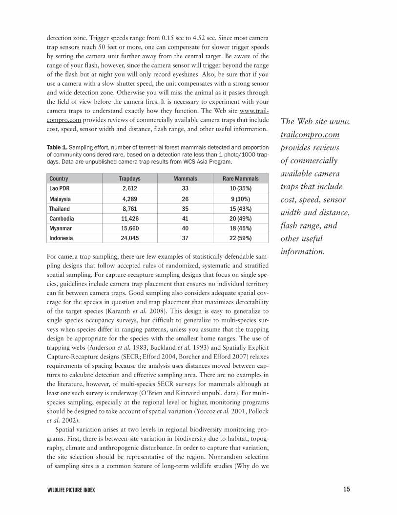
Sampling Design: equipment, effort, Time, SpacingYears of work in community ecology have taught us that the number of species detected is related to the area sampled and the sampling effort. Larger areas tend to have more species and as sampling effort increases, the number of rare species detected increases (Table 1). The size of the study site is an important consideration for estimating alpha diversity, since the area sampled should adequately represent the area used by the community of interest, including rare species (Buckland et al. 2005). As a general rule, sample points should be randomly or systematically assigned, and sampling should be sufficient at each point to provide a reasonable chance of detecting a species if it is present. It is important to keep the sampling quadrats of equal size for comparability.
For camera trapping studies, the sampling quadrats are analogous to the cam-era trap points and the quadrat size is measured as the area in which all individuals have a chance of being detected. The larger the sampling area, the more likely a species will be detected in the field of view. The sampling sensitivity or the abil-ity of a camera to capture a species that is in the field of view is determined by a combination of the field of view of the sensor (or detection zone), the distance that the sensor and camera can trigger, the trigger speed of the shutter, and, at night, the strength of the flash. Camera trap detection zones range from 345 ft2 to 4,185 ft2. Perhaps a more useful standard of comparison among camera traps is the field of view measured at 30 ft from the camera. Here we find that most camera traps have a field of view either in the range of 3 – 6 ft or they jump to a width of 26 ft. Clearly a camera with a wide field of view and a strong sensor will have a large
Dt ��2��t‐2��� 1��t‐1��� 2��t��� 1��t�1���2��t�2�
15WILDLIFE PICTURE Index
detection zone. Trigger speeds range from 0.15 sec to 4.52 sec. Since most camera trap sensors reach 50 feet or more, one can compensate for slower trigger speeds by setting the camera unit further away from the central target. Be aware of the range of your flash, however, since the camera sensor will trigger beyond the range of the flash but at night you will only record eyeshines. Also, be sure that if you use a camera with a slow shutter speed, the unit compensates with a strong sensor and wide detection zone. Otherwise you will miss the animal as it passes through the field of view before the camera fires. It is necessary to experiment with your camera traps to understand exactly how they function. The Web site www.trail-compro.com provides reviews of commercially available camera traps that include cost, speed, sensor width and distance, flash range, and other useful information.
For camera trap sampling, there are few examples of statistically defendable sam-pling designs that follow accepted rules of randomized, systematic and stratified spatial sampling. For capture-recapture sampling designs that focus on single spe-cies, guidelines include camera trap placement that ensures no individual territory can fit between camera traps. Good sampling also considers adequate spatial cov-erage for the species in question and trap placement that maximizes detectability of the target species (Karanth et al. 2008). This design is easy to generalize to single species occupancy surveys, but difficult to generalize to multi-species sur-veys when species differ in ranging patterns, unless you assume that the trapping design be appropriate for the species with the smallest home ranges. The use of trapping webs (Anderson et al. 1983, Buckland et al. 1993) and Spatially Explicit Capture-Recapture designs (SECR; Efford 2004, Borcher and Efford 2007) relaxes requirements of spacing because the analysis uses distances moved between cap-tures to calculate detection and effective sampling area. There are no examples in the literature, however, of multi-species SECR surveys for mammals although at least one such survey is underway (O’Brien and Kinnaird unpubl. data). For multi-species sampling, especially at the regional level or higher, monitoring programs should be designed to take account of spatial variation (Yoccoz et al. 2001, Pollock et al. 2002).
Spatial variation arises at two levels in regional biodiversity monitoring pro-grams. First, there is between-site variation in biodiversity due to habitat, topog-raphy, climate and anthropogenic disturbance. In order to capture that variation, the site selection should be representative of the region. Nonrandom selection of sampling sites is a common feature of long-term wildlife studies (Why do we
The Web site www.
trailcompro.com
provides reviews
of commercially
available camera
traps that include
cost, speed, sensor
width and distance,
flash range, and
other useful
information.
Table 1. Sampling effort, number of terrestrial forest mammals detected and proportion of community considered rare, based on a detection rate less than 1 photo/1000 trap-days. Data are unpublished camera trap results from WCS Asia Program.
Country Trapdays Mammals Rare MammalsLao PDR 2,612 33 10 (35%)
Malaysia 4,289 26 9 (30%)Thailand 8,761 35 15 (43%)Cambodia 11,426 41 20 (49%)Myanmar 15,660 40 18 (45%)Indonesia 24,045 37 22 (59%)

16 Wildlife Conservation Society | WORKING PAPER NO. 39
work where we work? Usually because of abundant wildlife!) and can lead to faulty inferences. For instance, a program based on monitoring wildlife in well-managed national parks may not tell us much about the region where those parks are located. However, many considerations lead us to make decisions about where to locate a sampling site, especially in the tropics. Given the practical limitations, non-random site location will continue to plague us and research into estimating regional trends when sample sites are non-random will continue to be an area of interest (Buckland et al. 2005). Within a sample site, there is also variation due to local habitat, micro-climatic, micro-topographic and anthropogenic disturbance. We usually have more control over sampling allocation within a site as opposed to between sites. A defendable sampling design should employ randomized or systematic assignment of sampling points to ensure representative coverage. Stratification by habitat or elevation may also be appropriate within a site.
Area of coverage at a sample site should ideally be determined by the dis-tribution of species in the community to be monitored; to adequately represent wide-ranging species, the area of coverage must be sufficiently large. Species with ranges that cover 10 – 50 km2 will require sampling at the level of hundreds of square kilometers. I propose sampling units of 200 km2 as a general rule of thumb. This size allows for the spatial coverage necessary to sample most large, wide-ranging species such as large cats and elephants. It is also a logistically fea-sible area to cover within the constraints of a single season, limited resources and under difficult field conditions.
Sampling intensity is usually measured in trapdays, a combination of num-ber of traps deployed and number of 24-hour periods of sampling. Camera trap sampling of rare species may require several thousand trapdays to develop an adequate number of encounters for analysis. To help plan a camera trap design for WPI based on occupancy analyses, I considered the tradeoffs between detection probability of a species, the expected area of occupancy, the number of days in a trapping season, and the number of points required to achieve relatively unbiased and precise occupancy estimates at the level of species. I assumed that the species in a community were a mix of rare species (detected after a minimum of 1,000 trapdays), common species, widely occurring species and spatially restricted species (only occurring at a few points in the sample). Since a composite index based on occupancy estimates inherits the bias and uncertainty of the species estimates that comprise the index, I looked for a sampling strategy that produces the most robust species occupancy estimates in terms of accuracy, precision and cost.
I considered a species with a range of detection probabilities (0.02, 0.03, 0.04, 0.06, 0.08, and 0.10), representative of the range of uncommonly to rarely encountered species. I considered a true occupancy of 10% to 60% of the sample points in 10% intervals. I then evaluated the limits of reliable detection for a range of sampling intensities (60 camera points to 100 camera points and 30 days of sampling/point). I considered an estimate as reliable when its bias was less than 10% of true value and its coefficient of variation (CV) was 20% or lower.
Table 2 shows that we can achieve acceptable accuracy using 60 camera points at a detection probability of 0.03 only for those species with 60% occu-pancy or greater. As we attempt to monitor species with lower detection prob-abilities and more restricted distribution, more camera points are required to
Nonrandom
selection of
sampling sites is
a common feature
of long-term
wildlife studies
and can lead to
faulty inferences.

17WILDLIFE PICTURE Index
accurately estimate occupancy within 30 days. Even 120 trap points are insuf-ficient to provide unbiased estimators when a species has a detection probability of 0.02 and occupancy of 20%.
Table 3 shows the effort required to gain acceptable precision for a range of detection probabilities and occupancies. It is much harder to increase precision (reduce CV) using 60 trap points. Even 100 trap points produce imprecise esti-mates for those species with the lowest detection probabilities.
Ideally, we would like to have precise and accurate occupancy estimates to enter into the WPI for all classes of detection and occupancy. Unfortunately, achieving the last 5% of gain can be prohibitively expensive. As a compromise between the time required to trap a large number of trap points, the cost of camera traps, cost of deployment in the field, and the large area to be covered, I recommend that 100 camera points across 200 km2, or 1 camera per 2 km2, be considered adequate coverage for a WPI survey. This is an arbitrary decision, but experi-ence in many WCS sites and in implementing WPI monitoring for the TEAM Program suggests that this is a feasible target that can be completed within 3-4 months, a reasonable length of time to consider a closed season for medium and large mammals and birds. Refining the understanding of the sampling require-ments for precise and unbiased WPI estimates is the topic of current analysis.
WPI surveys should be completed at each site on an annual basis. The time of year in which surveys are conducted is a site-level decision. The choice of
Table 2. Number of trap points operated for 30 days required to minimize bias (bias < 10%) for a range of detection probabilities, P.
True Occupancy
P=0.02 P=0.03 P=0.04 P=0.06 P=0.08 P=0.1
60% 70 60 60 60 60 6050% 80 70 60 60 60 6040% >100 80 60 60 60 6030% >100 100 60 60 60 6020% >100 >100 100 70 60 6010% >100 >100 100 80 80 80
Table 3. Number of trap points operated for 30 days required to minimize CV (CV < 20%) for a range of detection probabilities, P.
True Occupancy
P=0.02 P=0.03 P=0.04 P=0.06 P=0.08 P=0.1
60% >100 100 60 60 60 6050% >100 >100 70 60 60 6040% >100 >100 100 60 60 6030% >100 >100 >100 90 80 7020% >100 >100 >100 >100 >100 10010% >100 >100 >100 >100 >100 >100

18 Wildlife Conservation Society | WORKING PAPER NO. 39
season should be left up to the site managers for the camera trap protocol but, once a season is chosen, it should not change in future years. The deployment of cameras should be kept consistent (same season, same locations) over time at each site in order to control for seasonally-regulated influences on animal behavior, occupancy or abundance.
Strategies for camera trap deployment are difficult to prescribe so I will only give suggestions that have worked for researchers in the past. Most monitoring programs can afford to purchase 30 to 50 cameras at a time. Often, climatic con-ditions, theft, and wildlife damage can all take a toll on camera traps. Hot wet climates require camera traps that can withstand the weather, whereas in tropical savannah climates, less durable units may be used. Locks and theft-proof boxes can add expense to a monitoring program, but are a wise investment in human-dominated landscapes where theft of camera traps can be a problem.
I have envisioned that a researcher wishing to conduct a WPI survey would be able to deploy 33 – 35 cameras for a month in three sampling blocks totaling ~ 200 km2. The camera trap deployment rests on the assumption that each site will deploy 30-35 operating cameras during a sampling period (30 days) and that the cameras will not be visited until they are ready to be moved. The precise shape of each sample is dependent, to some extent, on landscape features and access, and the initial deployment of traps should be determined with GIS prior to going to the field (see Figure 4). I find it useful to determine the area to be trapped, and overlay a grid of the desired area to be sampled by a single point, generate centroid points for the grid and use these as the starting points for the sampling design. This can easily be done using ArcView or ArcGIS. Samples should be oriented along a gradient from disturbance to pristine conditions. For some sites, this will mean that the edge of disturbance is directly adjacent to the sample blocks. Other sites will have a buffer of undisturbed habitat before encountering an edge of disturbance. The spacing between cameras is sufficient to ensure that the sampling occurs at the level of habitat use by most or all of the largest mammals and birds in the community.
Practicalities of Setting Camera TrapsOnce the initial trapping design is established, the cameras should be deployed. The deployment team should use GPS to navigate to specific trap point coordi-nates and, once the deployment team reaches the sample point, they will need to find the best possible location as close as possible to the predetermined coordi-nates, preferably within 50 m but possibly within 100 m. The exact site is chosen to give the highest probability of obtaining useful photographs of a range of spe-cies, usually a game trail. The goal is to photograph as many species as possible. Although different species have different travel habits, and trail characteristics may affect the species that use those trails, local knowledge of the situation on the ground should assist in making the decision. Once the final location is chosen, the leader of the camera trap deployment team should record the new longitude and latitude coordinates of the final placement of the camera trap using a GPS unit. This serves as the permanent location of the camera trap point in all subsequent surveys.

19WILDLIFE PICTURE Index
It is difficult to give unambiguous recommendations for choosing the ideal sample point for a global, community-level monitoring program. Choice will depend on the habitat and animal community under consideration. A few tips that have been suggested in the past include:
Pick a site where the travel path is restricted to the area that can be photo-• graphed by the camera. For example, a good location to place a camera trap could be a place where there is a good deal of wildlife sign or an intersection of several trails. A single trail with evidence of wildlife use and limited travel alternatives is optimal for placing cameras. The maximum trail width should be less than the flash distance; we recommend no more than 15-20 ft. The ground and slope under the sensor beam needs to be reasonably level. • Trails with ruts or holes in front of the camera may inhibit use, especially if they fill with water after rains. Slopes can result in the ground obscuring ani-mals from the sensor beams. A pronounced slope on one side of the path may result in a sensor beam that is at shoulder height of large mammals but over the heads of smaller animals on the down slope. Be aware of all the possibili-ties of travel in front of the cameras. The best way to do this is to test cameras for the ability to detect animals with a shoulder height of 20-50 cm.
The goal is to
photograph as
many species as
possible.
Figure 4. An example of a basic design for deploying camera trap across a 200 km2 landscape in a systematic grid that ensures a spacing of 1 camera per 2 km2. Points represent camera trap locations. Dark line is boundary of landscape, and light lines represent a road system.

20 Wildlife Conservation Society | WORKING PAPER NO. 39
Increasingly, camera trap projects are converting to digital camera traps. It is critically important that projects organize data management in a careful manner. I recommend a catalogue of directories that begin at the site level, blocks within sites, points within blocks, cameras within points, discs within cameras and pho-tographs within discs. The TEAM network has produced a terrestrial vertebrate monitoring protocol that provides detailed advice for camera deployment and data management (available for download at www.teamnetwork.org)
Date & Time SettingsPhotographs without an accurate date and time stamp are practically useless. The date on the photograph is essential for determining the individual capture event for occupancy analysis. Each 24-hour period is considered one of 30 sampling periods so that all pictures of an individual photographed on the same date occur within a single capture period. If you wish to use a filter to determine which photographs constitute independent events (O’Brien et al. 2003), then the time stamp can be used to distinguish adjacent film frames taken 1 minute apart versus 1 hour apart. While camera models may differ slightly in setting the time/date stamp the important consideration is that it is consistent among all cameras in the monitoring program. Digital cameras allow the option of multiple frames per trigger event. This may be useful to help in identification of species.
Time DelaysAll camera traps can be programmed with a delay between successive pictures. This is important as group-living species or animals that linger in front of the camera can result in many wasted pictures, and more importantly, fill the memory card or deplete the battery before the sampling period is finished. A non-function-ing camera creates a data gap in the survey design that may result in the loss of data. The delay setting should be based upon the likelihood of encountering large groups of non-target animals: experimentation during the pilot study period will assist in selecting the length of the delay setting for your study site. Because a lon-ger delay increases the probability of missing a capture, the rule of thumb should be to use the minimum length of delay you feel comfortable with. For instance, a 2 GB flashcard can store 3,000 images or more so the trigger interval is not a large concern so long as you do not have false triggers due to moving vegetation. For the WPI, a setting of 1 minute between triggers is appropriate to detect spe-cies. This will reduce the number of photos of group-living species passing by the camera, yet allows classification of independent photo events.
Setting the Camera TrapsOnce all these factors have been considered and the optimal sample point loca-tion is determined, the camera traps must be set. Find a location where there is a suitable tree or insert a post at an optimal site. Suitable trees have trunks that are reasonably straight, thin enough to tie a chain or wire around, but not so thin that wind, people or other animals can shake it excessively. Try to minimize direct sunlight on the cameras as excessive heat can reduce the sensitivity of the sensors to endothermic animals. It is important to avoid setting a camera fac-ing east or west as the sunset and sunrise may cause glare on the photograph. Cameras should be set back at least two meters from the nearest point where an

21WILDLIFE PICTURE Index
animal might travel across the sensor. This allows for clear, focused pictures and a large field of detection from the sensor. The longer an animal is in the detection zone, the less chance of missing a photograph. Because the sensor beam should be approximately shoulder-high on the average target species, the camera should be set approximately 30-50 centimeters off the ground and parallel to it. Once a camera is positioned, the details of positioning should be recorded and referred to in subsequent sampling. The camera should be mounted to face perpendicular to the trail. Use pliable, light gauge wire, rubber or elastic cords, or suitable strap-ping material to secure the cameras to the selected tree trunk. The camera should be tightly mounted so that it does not move unless considerable force is applied. If locks and chains (or bicycle lock) are necessary to secure the cameras against theft, wait until cameras have been tightened with the wire before securing them. A twig or wedge placed between the camera housing and the tree trunk can help adjust the angle in which the sensor is pointed.
Once the camera is positioned, clear the area between the camera and the path of travel of all vegetation. Anything that obstructs the beam reduces the detection ability of the camera, and could result in obscured pictures. Large leaves and blades of grass can result in false triggers when the sun heats up a frond blowing in the wind. Also try to avoid pointing the cameras at objects in direct sunlight that may absorb heat and trigger sensors such as large rocks or sunlit streams. Be aware of the field of view for the camera and the sensor, and be sure that both fields of view are clear.
Test the aim of the sensor by crossing in front of it. Do this on both the near and far edge of the trail as well as the middle of the trail. Most camera trap brands come equipped with an indicator light that will light up when the cam-era’s sensor makes detection. Approximate a typical target species by walking in a crouch or crawling past the sensor. Make sure that every angle at which an animal can pass in front of the camera is tested, and that in each instance the sensor is triggered.
Occasionally, limitations in terrain or suitable trees hamper complete cov-erage of a trail. In such cases, lay brush or other obstructions down one side of the trail to restrict the travel path and guide animals past the camera. This technique is also useful if you are unable to set the camera well back from the trail, and wish to deter an animal from passing so closely to a camera that it cannot take a well-focused picture.
Once the camera is positioned and the field of view is clear, activate the camera. If you rely on a camera with normal flash, be sure the flash is set to activate every time the camera triggers, and that the red-eye and other features that slow the flash or trigger are turned off. Be sure that the date and time stamp are activated and properly set. To be sure that film are not later mixed, it is useful to use the first frame of the film to identify the film number. This can be done by photographing a white board with the film number clearly written in large numerals. If you do this, activate the flash after the white board picture. Some teams photograph themselves using their fingers to indicate film number (4 people; one's fingers to represent thousands, one's hundreds, one's tens and one's the final digit [1-9]). If you use digital cameras, some models allow additional information to be programmed into the EXIF file that stores metadata for each image. Camera point can be pro-grammed and later the metadata can be exported using a variety of software.

22 Wildlife Conservation Society | WORKING PAPER NO. 39
Monitoring the CamerasThe amount of animal traffic, human disturbance, and sensitivity of the camera trap sensor will dictate how fast the camera memory fills. Film cameras should probably be checked once a week if possible. In Sumatran forests, we left film cameras for 30 days and most retained unexposed films (O’Brien et al. 2003). Ideally, a digital camera should not run out of memory during the sampling period. Given that 2GB flash cards may hold more than 2,000 images, it is unlikely that a digital camera should stop working unless it malfunctions, fires repeatedly, or unless animals linger in front of the camera for excessive amounts of time. Realistically, one might expect 10% of cameras to fail for a range of reasons or to use up the memory before the end of a 30-day sampling period. Careful positioning of cameras should minimize sensor misfires and careful maintenance should minimize mechanical or battery failure. It should not be necessary to service the camera during a 30-day sampling period.

23WILDLIFE PICTURE Index
Bibliography
Andam, K.S., P.J. Ferraro, A. Pfaff, G.A. Sanchez-Azofelfa and J.A. Robalino. 2008. Measuring the effectiveness of protected area networks in reducing defor-estation. PNAS 105:16089-16094.Anderson, D.R., K.P. Burnham, G.C. White and D.L. Otis. 1983. Density estimation of small-mammal populations using a trapping web and distance sampling methods. Ecology 64:674-80.Andelman, S.J. and M.R. Willig. 2003. Present patterns and future prospects for biodiversity in the Western Hemisphere. Ecological Letters 6:818-824.Baillie, J.E.M., B. Cullen, R. Amin, H.R. Akcakaya, S.H.M. Buchart, N Brummitt, T.R. Meagher, M. Ram, C. Hilton-Taylor and G.M. Mace. 2008. Toward monitoring global biodiversity. Conservation Letters 1:18-26.Balmford, A., A. Bruner, P. Cooper, R. Constanza, S. Farber, R.E. Green, et al. 2002. Economic reasons for conserving wild nature. Science 297:950-953.Balmford, A., P. Crane, A. Dobson, R.E. Green and G.M. Mace. 2005. The 2010 challenge: data availability, information needs and extraterrestrial insights. Phil. Trans. R. Soc. B. 360:221-228.Borcher, D.L. and M.G. Efford. 2007. Spatially explicit maximum likelihood methods for capture-recapture studies. Biometrics 63:1-9.Boulinear, T., J.D. Nichols, J.R. Sauer, J.E. Hines and K.P. Pollock. 1998. Estimating species richness: The importance of heterogeneity in species detect-ability. Ecology 79:1018-10288.Bruner, A.G., R.E. Gullison, R.E. Rice and G.A.B. da Fonsesca. 2001a. Effectiveness of parks in protecting tropical biodiversity. Science 291:125-128.Bruner, A.G., R.E. Gullison, R.E. Rice and G.A.B. da Fonsesca. 2001b. The effectiveness of parks: response. Science 293:1007a.Buckland, S.T., D.R. Anderson, K.P. Burnham and J.L. Laake. 1993. Distance Sampling: Estimation of Biological Populations. Chapman and Hall, New York. Buckland, S.T., A.E. Margurran, R.E. Green and R.M. Fewster. 2005. Monitoring change in biodiversity through composite indices. Phil. Trans. R. Soc. Lond. B. 360(1454): 243 – 254.Bunge, J. and M. Fitzpatrick. 1993. Estimmating the number of species: a review. J. Am. Stat. Assoc. 88:364-373.Butchart, S.H.M., A.J. Stattersfield, L.A. Bennun, S.M. Shutes, H.R. Akçakaya, J.E.M. Baillie, S.N. Stuart, C. Hilton-Taylor and G.M. Mace. 2004. Measuring global trends in the status of biodiversity: Red List Indices for birds. PLoS Biology 2:2294–2304.Butchart, S., H.R. Akçakaya, J. Chanson, J.E.M. Baille, B. Collen, S. Quader, W.R. Turner, R. Amin, S.N. Stuart and C. Hilton-Taylor. 2007. Improvements to the Red List Index. PLoS1 1:e140.Cam, E., J.D. Nichols, J.R. Sauer, J.E. Hines and C.H. Flather. 2000. Relative species richness and community completeness: Avian communities and urban-ization in the mid-Atlantic states. Ecol. Appl. 10:1196-1210.Conroy, M.J. 1996. Abundance indices. In: Measuring and Monitoring Biological Diversity: Standard Methods for Mammals (Wilson, D.E., Cole, F.R., Nichols, J.D., Rudran, R., and Foster, M.S., eds.), pp 179-192, Smithsonian Institution Press, Washington, D.C. Collen, B., M. Ram, T. Zamin and L. McRae. 2008. The tropical biodiversity data gap: addressing disparity in global monitoring. Tropical Conservation Science 1:75-88.
24 Wildlife Conservation Society | WORKING PAPER NO. 39
Collen, B., J. Loh, S. Whitmee, L. McRae, R. Amin and J.E.M. Baillie. 2009. Monitoring change in vertebrate abundance: the living planet index. Conserv. Biol. 23:317-327DeVries, R., A. Hansen, A.C. Newton and M.C. Hansen. 2005. Increasing iso-lation of protected areas in tropical forests over the past 20 years. Ecological Applications 15:19-26.Dobson. A. 2005. Monitoring global rates of biodiversity change: challenges that arise in meeting the Convention on Biological Diversity (CBD) 2010 goals. Phil. Trans. R. Soc. B. 360:229-241.Dobson, A., D. Lodge, J. Alder, G.S. Cumming, J. Keymer, J. McGlade, H. Mooney, J.A. Rusak, O. Sala, V. Wolters, D. Wall, R. Winfree and M.A. Xenopoulos. 2006. Habitat loss, trophic collapse, and the decline of ecosystem services. Ecology 87:1915-1924.Efford, M.G. 2004. Density estimation in live-trapping studies. Oikos 106:598–610.Ervin, J. 2003. Protected area assessments in perspective. BioScience 53:819-822.Fewster, R.M., S. T. Buckland, G.M. Siriwardena, S.R. Baillie and J.D. Wilson. 2000. Analysis of population trends for farmland birds using generalized addi-tive models. Ecology 81:1970-1984.Gregory, R.D., D. Noble, R. Field, J.H. Marchant, M. Raven and D.W. Gibbons. 2003. Using birds as indicators of biodiversity. Ornis Hungaria 12-13:11-14.Gregory, R.D., A. van Strien, P. Voβišek, A.W. Gmelig Meyling, D.G. Noble, R.P.B. Foppen and D.W. Gibbons. 2005. Developing indicators for European birds. Phil. Trans. R. Soc. B. 360:269-288.Gregory, R.D., P. Voβišek, D.G. Noble, A. van Strien, A Klcaβová, M. Eaton, A.W. Gmelig Meyling, A. Joys, R.P.B. Foppen and I.J. Burfield. 2008. The generation and use of bird population inidicators in Europe. Bird Conservation International 18:S223-S244.Hastie, T.J. and R.J. Tibshirani. 1990. Generalized Additive Models. Chapman and Hall, London, UK.Hollenbeck, J.P and W.J. Ripple. 2007. Aspen snag dynamics, cavity-nesting birds, and trophic cascades in Yellowstone’s northern range. Forest Ecology and Management 255:1095-1103.Hooper, D.U., F.S. Chapin III, J.J Ewel, A Hector, P. Inchausti, S. Lavorel, J.H Lawton, D.M. Lodge, M. Loreau, S. Naeem, B. Schmid, H. Setälä, A.J. Symstad, J. Vandemeer and D.A. Wardle. 2005. Effects of Biodiversity on ecosystem func-tioning: a consensus of current knowledge. Ecological Monographs 75:3-35.Joppa, L.N., S.R. Loarie and S.L. Pimm. 2008. On the protection of protected areas. PNAS 105:6673-6678.Karanth, K.U. and J.D. Nichols. 1998. Estimation of tiger densities in India using photographic captures and recaptures. Ecology 79: 2952-2862.Karanth, K.U. and J.D. Nichols, (eds.). 2002. Monitoring Tigers and Their Prey: A Manual for Researchers, Managers, and Conservationists in Tropical Asia. Centre for Wildlife Studies, Bangalore, India.Karanth, K.U. N.S. Kumar, V. Srinivas and A. Gopalaswamy. 2008. Revised Monitoring Framework for Tigers Forever-Panthera sites. Unpublished report to the Wildlife Conservation Society. 17 pp.Kelly, M.J., A.J. Noss, L.R. Arispe, M. Di Bitetti, C.D. De Angelo, A. Paviolo, Y.E. Di Blanco and L. Maffei. 2008. Estimating puma densities from remote cameras across three study sites: Bolivia, Argentina, and Belize. J. Mammal. 89: 408-418.Limpert, E., W.A. Stahel and M. Abbt. 2001. Log-normal distributions across the sciences: keys and clues. Bioscience 51: 341-352.

25WILDLIFE PICTURE Index
Loh, J., R.E. Green, T. Ricketts, J. Lamoreux, M. Jenkins, V. Kapos and J. Randers. 2005. The Living Planet Index: using species population time series to track trends in biodiversity. Phil. Trans. R. Soc. 360:289-295.Mace, G. M. and J. E. M. Baillie. 2007. The 2010 Biodiversity Indicators: chal-lenges for science and policy. Conservation Biology 21:1406-1413.MacKenzie, D.I. and J.A. Royle. 2005. Designing occupancy studies: general advice and allocating survey effort. Ecol. Appl. 42:1105-1114.MacKenzie, D.I., Nichols, J.D., Royle, J.A., Pollock, K.P., Bailey, L.L. and Hines, J.E. 2006. Occupancy Estimation and Modeling: Inferring Patterns and Dynamics of Species Occurrence. Academic Press, New York.Magurran, A.E. 2004. Measuring Biological Diversity. Oxford: Blackwell Science.Meir, E., S. Andelman and H.P. Possingham. 2004. Does conservation planning matter in a dynamic and uncertain world. Ecology Letters 7:615-622.Millenium Ecosystem Assessment. 2005. Ecosystems and Human Well-being: A Framework for Assessment. Island Press, Washington, D.C.Norton-Griffiths, M. 2007. How many wildebeest do you need? World Economics 8:41-64.O’Brien, T.G. 2008. On the use of automated cameras to estimate species rich-ness for large- and medium-sized rainforest mammals. Animal Conservation 11:179-181.O’Brien, T.G. and M.F. Kinnaird. 2008. A picture is worth a thousand words: the application of camera trapping to the study of birds. Bird Conservation International 18: S144-S162.O’Brien, T.G., M.F. Kinnaird and H.T. Wibisono. 2003. Crouching tigers, hid-den prey: Sumatran tiger and prey populations in a tropical forest landscape. Anim. Cons. 6:131-139.O’Brien, T.G., H.T. Wibisono and M.F. Kinnaird. In press. Species richness estimation using camera traps: An Indonesian example. In: Camera Traps in Animal Ecoclogy: Methods and Analyses (O’Connell, A.F., Nichols, J.D., and Karanth, U.K. eds.), Springer Tokyo Inc.Odling-Smee, L. 2005. Dollars and sense. Nature 436:614-616.Parrish, J.D., D.P. Braun and R.S. Unnasch. 2003. Are we conserving what we say we are? Measuring ecological intergrity within protected areas. BioScience 53:851-860.Pimm, S.L., H.L. Jones and J. Diamond. 1988. On the risk of extinction. American Naturalist 132:757–785. Pimm, S.L., G.J. Russell, J.L Gittleman and T.H. Brooks. 1995. The future of biodiversity. Science 269:347-350.Pollock, K.H., J.D. Nichols, T.R. Simons, G.L. Farnsworth, L.L. Bailey and J.R. Sauer. 2002. Large scale wildlife monitoring studies: statistical methods for design and analysis. Environmetrics 13:105-119. Power, M.E., D. Tilman, J. Estes, B.A. Menge, W.J. Bond, L.S. Mills, G. Daily, J.C. Castilla J. Lubchenco and R.T. Paine. 1996. Challenges in the quest for keystones. BioScience 46:609-620.Pringle, R.M., T.P. Young, D.I. Rubenstein and D.J. McCauley. 2007. Herbivore-initiated interaction cascades and their modulation by productivity in an African savanna. PNAS 104:193-197.Purves, A., K.E. Jones and G.M. Mace. 2000. Extinction. Bioessays 22:1122-1133.Raffaelli, D. 2004. How extinction patterns affect ecosystems. Science 306:1141-1142.Ray, J.C. 2005. Large carnivorous animals as tools for conserving biodiver-

26 Wildlife Conservation Society | WORKING PAPER NO. 39
sity: assumptions and uncertainties. Pp. 34-56 In: Large Carnivores and the Conservation of Biodiversity. J.C. Ray, K.H. Redford, R.S. Steneck and J. Berger (eds.) Island Press, Washington, D.C.Ripple, W.J. and R.L Beschta. 2004. Wolves, elk, willows and trophic cascades in the upper Gallitin range of southwestern Montana, USA. Forest Ecology and Management 200:161-181.Rodrigues, A.S.L., H.R. Akçakaya, S.J. Andelman, M.I. Bakaar, L. Boitani, T.M. Brooks, J.S. Chanson, L.D.C. Fishpool, G.A.B. Da Fonseca, K.J. Gaston, M.Hoffman, P.A. Marquet, J.D. Pilgrim, R.L. Pressey, J. Schipper, W. Secrest, S.N. Stuart, L.G. Underhill, R.W. Waller, M.E.J. Watts and X. Yan. 2004. Global gap analysis: priority regions for expanding the global preotected-area network. BioScience 54:1092-1100.Rowcliffe, J.M. and C. Carbone. 2008. Surveys using camera traps: are we looking to a brighter future? Animal Conservation 11:185-186.Silver, S.C., L.E.T. Ostro, L.K. Marsh, L. Maffei, A.J. Noss, M.J. Kelly, R.B. Wallace, H. Gómez and G. Ayala. 2004. The use of camera traps for estimating jaguar Panthera onca abundance and density using capture/recapture analysis. Oryx 38: 148-154.Solan, M., B.J. Cardinale, A.L. Downing, K.A.M. Engelhardt, J.L. Ruesink and D.S. Srivastava. 2004. Extinction and ecosystem function in the marine benthos. Science 306:1177-1180.Terborgh, J., L. Lopez, P. Nuñez, M. Rao, G. Shahabuddin, G. Orihuela, M. Riveros, R. Ascanio, G.H. Adler, T.D. Lambert and L. Balbas. 2001. Ecological meltdown in Predator-free forest fragments. Science 294:1923-1926.Tobler, M.W., S.E. Carrilo-Percastegui, R.L. Pitman and G. Powell. 2008a. An evaluation of camera traps for inventorying large and medium sized terrestrial rainforest mammals. Animal Conservation 11:169-178.Tobler, M.W., S.E. Carrilo-Percastegui, R.L. Pitman, R. Mares and G. Powell. 2008b. Further notes on the analysis of mammal inventory data collected with camera traps. Animal Conservation 11:187-189.Vanclay, J.K. 2001. The Effectiveness of parks. Science 293:1007a.Wood, S. 2006. Generalized Additive Models. An Introduction with R. Chapman and Hall/CRC, Boca Raton, Fl.Yoccoz, N.G., J.D. Nichols and T. Boulinier. 2001. Monitoring of biological diversity in space and time. TREE 16:446-453.Zar, J.H. 1999. Biostatistical Analysis: Fourth Edition. Prentice Hall, Upper Saddle River, New Jersey, USA.Zavaleta, E.S. and K.H. Hulvey. 2004. Realistic species losses disproportionately reduce grassland resistance to biological invaders. Science 306:1175-1177.
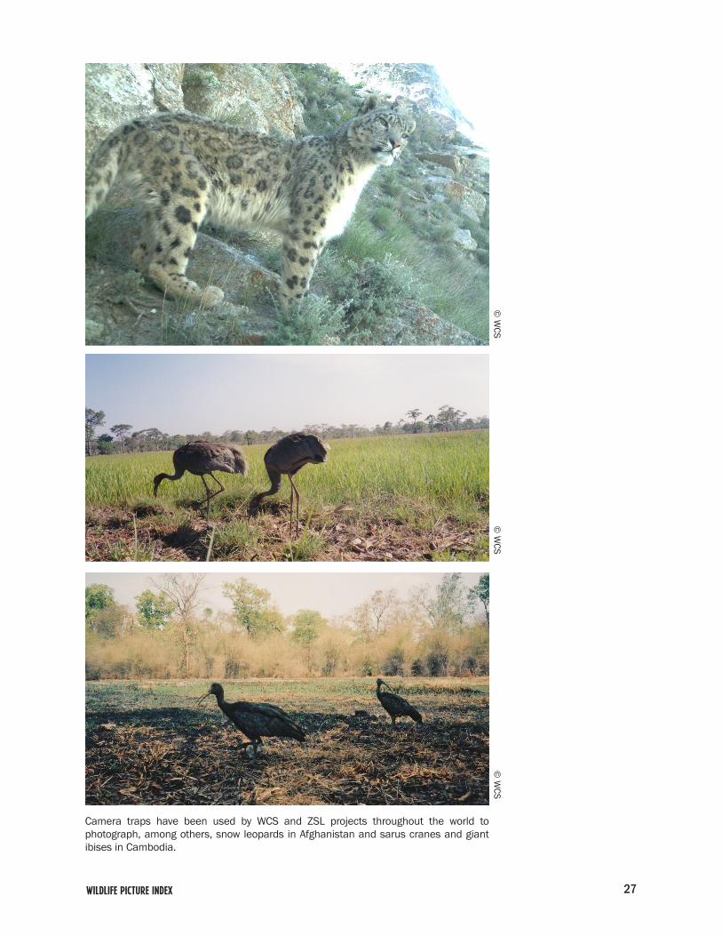
27WILDLIFE PICTURE Index
Camera traps have been used by WCS and ZSL projects throughout the world to photograph, among others, snow leopards in Afghanistan and sarus cranes and giant ibises in Cambodia.
© W
CS©
WCS
© W
CS
28 Wildlife Conservation Society | WORKING PAPER NO. 39
Model specification using generalized additive Models. From Fewster et al. (2000), with permission of r. Fewster and S. Buckland.
Generalized additive models (GAMs) are flexible extensions of general linear mod-els (GLMs). We assume that the counts yit follow independent Poisson distribu-tions, with mean μit for the count in site i in year t. However, the linear predictor associated with the GLM, is replaced by a more general additive predictor. This allows the change in mean abundance over time to follow any smooth curve, not just a linear form as in linear regression or a sequence of unrelated estimates as in log-linear Poisson regression. The form of the predictor function is the principal difference between the GLM and the GAM. We write the additive predictor as
log(μit) = αi + f(t)
The expected count μit in site i in year t therefore depends upon the site effect αi, and upon any number of other smoothly varying quantities, which are summarized by the value f(t) in year t. The notation f(t) simply represents any smooth function of time. The GAM is fitted by estimating the parameters αi and the smooth function f. There are two special cases of the GAM formu-lation that fall into the category of GLMs. The first is the simple linear trend model, in which f(t) = γt for a single parameter γ to be estimated. In this case, the expected abundance within each site varies linearly on a logarithmic scale with time. The second case is the log-linear Poisson regression model for which f(t) = βt for parameters β1, . . . , βT to be estimated. In this instance, the function f is no longer smooth, and is obtained by joining the estimates βt with straight lines. These two cases lie at opposite extremes of the GAM framework. The first has maximum smoothness in the function f, a single straight line; the second has minimum smoothness, a sequence of unconstrained estimates joined by lin-ear segments. Between the two extremes lie functions s with greater flexibility than the linear trend f(t)=γt, but with smooth output in contrast to the discrete annual estimates f(t) = βt. These intermediate GAM curves provide opportuni-ties for eliciting long-term nonlinear trends that are not available at the GLM extremes.
The output from the GAM is visualized as follows. The fitted year effect curve f(t) is common to all sites, so that for any two sites i1 and i2, the curves log(μi1t)
APPENDIX 1
^

29WILDLIFE PICTURE Index
and log(μi2t) are parallel. The intercepts of these curves are determined by the site effects, respectively αi1 and αi2. Consequently, every site is subject to the same trend in the logarithm of expected count over time, although the absolute values differ between sites. The assumption that log abundance follows the same trend in every site, although simplistic, is the same as that implicit in the traditional Poisson regression models. Indeed, the assumption is perhaps better justified in the GAM context, because it is more reasonable to suggest that there is a smooth pattern of change common to all sites than to assert that all sites are subject to the same series of annual fluctuations. Nonetheless, the GAM system also accommodates models that allow trends to vary between different regions, or even within every site.
Once an estimate f has been obtained for the smooth function f, the annual abundance index curve I(t) is calculated as:
Before the function f can be estimated, the required level of smoothing must be established. At the two extremes of maximum and minimum smoothing, where the GAM is equivalent to a GLM, it is possible to specify f in parametric form: namely f(t) = γt at the upper extreme and f(t) = βt at the lower. Between these extremes, however, the function f is not defined in terms of parameters, but is estimated nonparametrically from the data by means of scatterplot smoothers. The shape of the function is therefore determined by the data rather than being restricted to a parametric form. Note the distinction between the smoothing procedures in a GAM, which are part of the model-fitting process, and the smoothing of Mountford or TRIM indices in a second step after the fit is complete.
Several options are available for the scatterplot smoother used in estimating f, although experimence suggests that the choice has little effect on the final index curve. All of the analyses presented in Fewster et al. (2000) were con-ducted using smoothing splines; other options include locally weighted regres-sion smoothers, kernel smoothers, and running-median smoothers.
Smoothing splines fit the data using piecewise cubic polynomials. They are chosen to satisfy a penalized least squares criterion, which optimizes the fit while penalizing roughness to some pre-specified extent. The extent to which roughness is penalized, or equivalently the level of smoothing that is applied, is calibrated by a quantity known as the degrees of freedom (df). As the degrees of freedom are increased, the function f gains in flexibility: more turning points and gradient changes are accommodated. A straight line f(t) = γt corresponds to a fit with 1 df; the curve follows a single direction only, with no gradient changes or turning points. Conversely, a piecewise linear fit f(t) = βt (t = 1, . . . , T) employs T - 1 df; a separate gradient is allowed between every successive pair of points. The degrees of freedom associated with the curve f may take any value between 1 and T - 1, and are loosely interpreted as the number of parameters used in fitting f.
The choice of the value for df is an important part of the modeling process. For clarity, we shall write fd for the curve f to be fitted using a smoothing spline on the variable t with d degrees of freedom, and we shall refer to the associated model as a ‘‘GAM with d degrees of freedom.’’ The choice of d depends largely
))1(ˆexp(
))(ˆexp(1
)(f
tfyearforcountpredictedtotal
tyearforcountpredictedtotaltI ==
^

30 Wildlife Conservation Society | WORKING PAPER NO. 39
on the objectives of the analysis. For inference about long-term trends, a smooth index curve is required, corresponding to low df; whereas information about annual fluctuations requires unconstrained annual estimates and the maximum value of d. Consideration of the length of the time series is also important, because longer time series will demand higher values of d if it is required to maintain a given level of flexibility in the trend curve.
Certain conceptual difficulties enter at this point, because it is not possible to assert that a GAM with df = a is more realistic than a GAM with df = b. The GAMs separate underlying trend from short-term fluctuation, but the pre-cise point at which a signal can be considered fluctuation rather than trend is ill-defined. The specification of df effectively represents models with different criteria for achieving this separation of trend from noise, and there is no right answer against which to judge them. To overcome this difficulty, it is necessary to formulate our own ideas about a reasonable definition of noise and trend. As d is raised from a low starting value, the index curve begins to reveal new features as it more closely tracks the data, but still remains smooth until a period of stability is reached. Further increases in d serve only to roughen the output. It is reasonable to take those points at which the output has stabilized, but is still smooth, as our definition of true trend. Experiments with trunca-tion of Common Birds Census data suggested that a value for d of roughly 0.3 times the length of the time series tended to produce trend curves with suitable complexity and smoothness, although we stress that advice will vary according to precise objectives and data. It is always necessary to plot indices from GAMs with a range of df before settling on a final value.
Automatic selection of the value of df in a generalized additive model is sometimes recommended, using, for example, Akaike’s Information Criterion (AIC) or generalized cross-validation. Each automatic procedure produces a sin-gle value of d that is optimal with respect to some criterion. Because the quan-tity optimized might be very different from our own requirements of the model, however, we do not recommend the use of automatic selection procedures in the context of trend analysis. For example, we might wish to examine the same data both for longterm trends and for information about annual fluctuations. Although different values of d are clearly required for the two purposes, an automatic selection routine would be unable to distinguish between the distinct objectives, and would provide the same value for both.
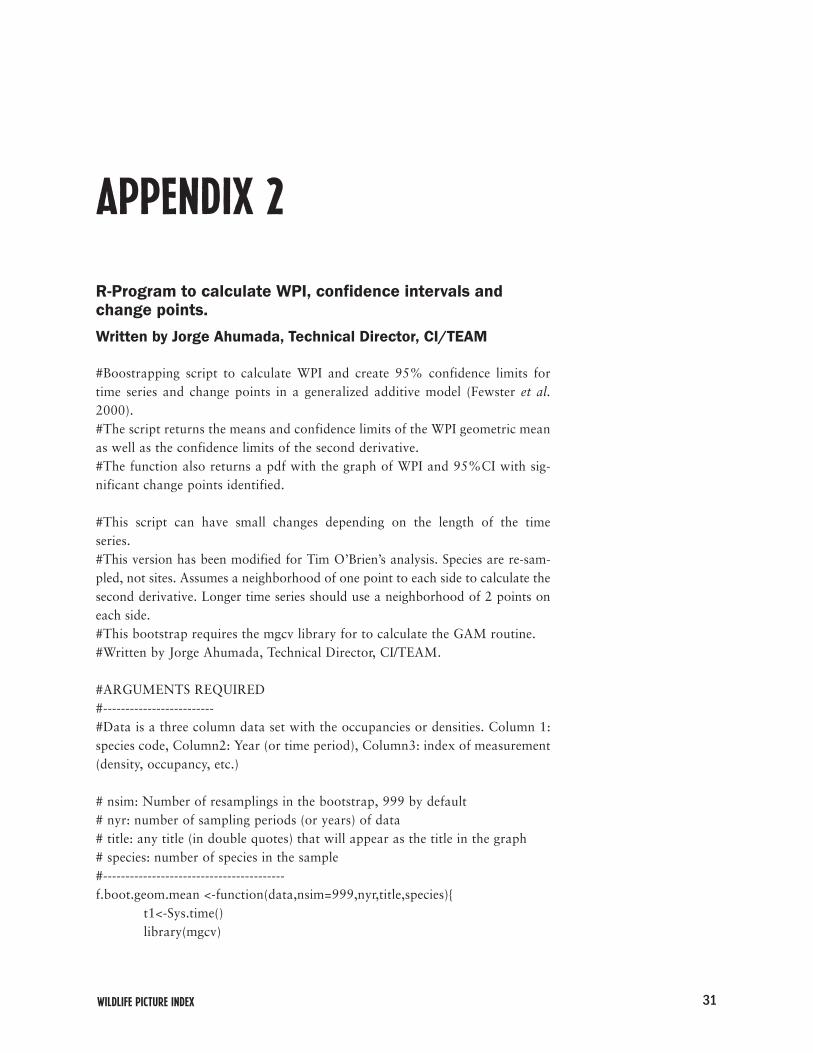
31WILDLIFE PICTURE Index
r-Program to calculate WPi, confidence intervals and change points. Written by Jorge ahumada, Technical Director, Ci/TeaM
#Boostrapping script to calculate WPI and create 95% confidence limits for time series and change points in a generalized additive model (Fewster et al. 2000).#The script returns the means and confidence limits of the WPI geometric mean as well as the confidence limits of the second derivative.#The function also returns a pdf with the graph of WPI and 95%CI with sig-nificant change points identified.
#This script can have small changes depending on the length of the time series.#This version has been modified for Tim O’Brien’s analysis. Species are re-sam-pled, not sites. Assumes a neighborhood of one point to each side to calculate the second derivative. Longer time series should use a neighborhood of 2 points on each side. #This bootstrap requires the mgcv library for to calculate the GAM routine.#Written by Jorge Ahumada, Technical Director, CI/TEAM.
#ARGUMENTS REQUIRED#-------------------------#Data is a three column data set with the occupancies or densities. Column 1: species code, Column2: Year (or time period), Column3: index of measurement (density, occupancy, etc.)
# nsim: Number of resamplings in the bootstrap, 999 by default# nyr: number of sampling periods (or years) of data# title: any title (in double quotes) that will appear as the title in the graph# species: number of species in the sample#----------------------------------------- f.boot.geom.mean <-function(data,nsim=999,nyr,title,species){ t1<-Sys.time() library(mgcv)
APPENDIX 2
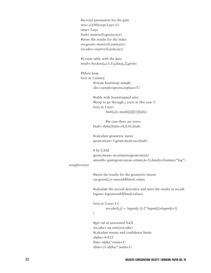
32 Wildlife Conservation Society | WORKING PAPER NO. 39
#several parameters for the gam wts<-c(1000,rep(1,nyr-1)) time<-1:nyr btab<-matrix(0,species,nyr) #store the results for the index res.geom<-matrix(0,nsim,nyr) res.sder<-matrix(0,nsim,nyr) #Create table with the data mtab<-by(data[,c(3,1)],data[,2],print) #Main loop for(i in 1:nsim){ #create bootstrap sample idx<-sample(species,replace=T) #table with bootstrapped sites #loop to go through j years in this case 5. for(j in 1:nyr) btab[,j]<-mtab[[j]][[1]][idx] #in case there are zeros btab<-ifelse(btab==0,0.01,btab) #calculate geometric mean geom.mean<-f.geom.mean.occ(btab) # fit GAM geom.mean<-as.numeric(geom.mean) smooth<-gam(geom.mean~s(time,k=3),family=Gamma(“log”),weights=wts) #store the results for the geometric means res.geom[i,]<-smooth$fitted.values #calculate the second derivative and store the results in res.sdr logsm<-log(smooth$fitted.values) for(j in 2:(nyr-1)) res.sder[i,j] <- logsm[j-1]-2*logsm[j]+logsm[j+1] } #get rid of unwanted NaN res.sder<-na.omit(res.sder) #calculate means and confidence limits alpha<-0.025 llim<-alpha*(nsim+1) ulim<-(1-alpha)*(nsim+1)

33WILDLIFE PICTURE Index
mean.smooth<-apply(res.geom,2,mean) ci.mean<-apply(res.geom,2,sort) ci.mean.lo<-ci.mean[llim,] ci.mean.hi<-ci.mean[ulim,] #calculate the 95% ci of the second derivative ci.der<-apply(res.sder[,2:(nyr-1)],2,sort) lo.ci.der<-c(rep(NA,1),ci.der[llim,],rep(NA,1)) hi.ci.der<-c(rep(NA,1),ci.der[ulim,],rep(NA,1)) range.der<-rbind(lo.ci.der,hi.ci.der) #figure out which symbols to use in the plot change.sign<-apply(range.der,1,x<-function(x){ifelse(x<0,1,2)}) change.sign<-apply(change.sign,1 ,sum) symbols<-ifelse(change.sign==2,25,ifelse(change.sign==4,24,19)) colors<-ifelse(symbols==25,”red”,ifelse(symbols==24,”green”,”black”)) name<-”graphs/results.” name<-paste(name,title,”.pdf”,sep=””) pdf(file=name,w=8,h=6) #plot the whole thing and put in a pdf plot(time,mean.smooth,xlab=”time”,ylab=”geometric mean of relative abundance”, ylim=range(ci.mean.lo,ci.mean.hi,na.rm=T),t=’p’,pch=symbols, cex=1,col=colors) lines(ci.mean.lo,lty=2) lines(ci.mean.hi,lty=2) lines(mean.smooth,pch=””,t=’b’) title(title) dev.off()
t2<-Sys.time() print(difftime(t2,t1,”min”)) #return result matrices list(smooth=mean.smooth,cimean=rbind(ci.mean.lo,ci.mean.hi),ci.change=range.der) }#END OF THE PROGRAM
#Function to calculate the geometric mean f.geom.mean.occ <- function(data){ apply(data,2,function(x) exp(1/length(data[,1])*sum(log(x/data[,1])))) }

34 Wildlife Conservation Society | WORKING PAPER NO. 39
WCS WORKING PAPER SERIESWCS Working Paper no. 1Bleisch, William V. (1993) Management Recommendations for Fanjing Mountain Nature Reserve and Conservation at Guizhou Golden Monkey & Biodiversity.
WCS Working Paper no. 2Hart, John A. and Claude Sikubwabo. (1994) Exploration of the Maiko National Park of Zaire, 1989-1994, History, Environment and the Distribution and Status of Large Mammals.
WCS Working Paper no. 3Rumiz, Damian and Andrew Taber. (1994) Un Relevamiento de Mamíferos y Algunas Aves Grandes de la Reserva de Vida Silvestre Ríos Blanco y Negro, Bolívia: Situación Actual y Recomendaciones.
WCS Working Paper no. 4Komar, Oliver and Nestor Herrera. (1995) Avian Density at El Imposible National Park and San Marcelino Wildlife Refuge, El Salvador.
WCS Working Paper no. 5Jenkins, Jerry. (1995) Notes on the Adirondack Blowdown of July 15th, 1995: Scientific Background, Observations, and Policy Issues.
WCS Working Paper no. 6Ferraro, Paul, Richard Tshombe, Robert Mwinyihali, and John Hart. (1996) Projets Integres de Conservation et de Developpement; un Cadre pour Promouvoir la Conservation et la Gestion des Ressources Naturalles.
WCS Working Paper no. 7Harrison, Daniel J. and Theodore G. Chapin. (1997) An Assessment of Potential Habitat for Eastern Timber Wolves in the Northeastern United States and Connectivity with Occupied Habitat on Southeastern Canada.
WCS Working Paper no. 8Hodgson, Angie. (1997) Wolf Restoration in the Adirondacks? The Question of Local Residents.
WCS Working Paper no. 9Jenkins, Jerry. (1997) Hardwood Regeneration Failure in the Adirondacks: Preliminary Studies of Incidence and Severity.
WCS Working Paper no. 10García Víques, Randall. (1996) Propuesta Técnica de Ordenamiento Territorial con Fines de Conservación de Biodiversidad en Costa Rica: Proyecto GRUAS.
WCS Working Paper no. 11Thorbjarnarson, John and Alvaro Velasco. (1998) Venezuela’s Caiman Harvest Program: A Historical Perspective and Analysis of its Conservation Benefits.
WCS Working Paper no. 12Bolze, Dorene, Cheryl Chetkiewicz, Qui Mingjiang, and Douglas Krakower. (1998) The Availability of Tiger-Based Traditional Chinese Medicine Products and Public Awareness about the Threats to the Tiger in New York City’s Chinese Communities: A Pilot Study.
WCS Working Paper no. 13O’Brien, Timothy, Margaret F. Kinnaird, Sunarto, Asri A. Dwiyahreni, William M. Rombang, and Kiki Anggraini. (1998) Effects of the 1997 Fires on the Forest and Wildlife of the Bukit Barisan Selatan National Park, Sumatra.

35WILDLIFE PICTURE Index
WCS Working Paper no. 14McNeilage, Alistair, Andrew J. Plumptre, Andy Brock-Doyle, and Amy Vedder. (1998) Bwindi Impenetrable National Park, Uganda. Gorilla and Large Mammal Census, 1997.
WCS Working Paper no. 15Ray, Justina C. (2000) Mesocarnivores of Northeastern North America: Status and Conservation Issues.
WCS Working Paper no. 16Kretser, Heidi. (2001) Adirondack Communities and Conservation Program: Linking Communities and Conservation Inside the Blue Line.
WCS Working Paper no. 17Gompper, Matthew E. (2002) The Ecology of Coyotes in Northeastern North America: Current Knowledge and Priorities for Future Research.
WCS Working Paper no. 18Weaver, John L. (2001) The Transboundary Flathead: A Critical Landscape for Carnivores in the Rocky Mountains.
WCS Working Paper no. 19Plumptre, Andrew J., Michel Masozera, Peter J. Fashing, Alastair McNeilage, Corneille Ewango, Beth A. Kaplin, and Innocent Liengola. (2002) Biodiversity Surveys of the Nyungwe Forest Reserve in S.W. Rwanda.
WCS Working Paper no. 20Schoch, N. (2003) The Common Loon in the Adirondack Park: An Overview of Loon Natural History and Current Research.
WCS Working Paper no. 21Karasin, L. (2003) All-Terrain Vehicles in the Adirondacks: Issues and Options.
WCS Working Paper no. 22Clarke, Shelly. (2002) Trade in Asian Dry Seafood, Characterization, Estimation and Implications for Conservation.
WCS Working Paper no. 23Mockin, Miranda H., E.L. Bennett, and D.T. LaBruna. (2005) Wildlife Farming: A Viable Alternative to Hunting in Tropical Forests?
WCS Working Paper no. 24Ray, Justina C., Luke Hunter, and Joanna Zigouris. (2005) Setting Conservation and Research Priorities for Larger African Carnivores.
WCS Working Paper no. 25Redford, Kent H. and Michael Painter. (2006) Natural Alliances Between Conservationists and Indigenous Peoples.
WCS Working Paper no. 26Agrawal, Arun and Kent Redford. (2006) Poverty, Development, and Biodiversity Conservation: Shooting in the Dark?
WCS Working Paper no. 27Sickler, Jessica, John Fraser, Sarah Gruber, Paul Boyle, Tom Webler, and Diana Reiss. (2006) Thinking About Dolphins Thinking.
WCS Working Paper no. 28Castillo, Oscar, Connie Clark, Peter Coppolillo, Heidi Kretser, Roan McNab, Andrew Noss, Helder Quieroz, Yemeserach Tessema, Amy Vedder, Robert Wallace, Joseph Walston, and David Wilkie. (2006) Casting for Conservation Actors: People, Partnerships and Wildlife.
WCS Working Paper no. 29Redford, Kent H. and Eva Fearn, eds. (2007) Protected Areas and Human Displacement: A Conservation Perspective.

36 Wildlife Conservation Society | WORKING PAPER NO. 39
WCS Working Paper no. 30Redford, Kent H., and Eva Fearn, eds. (2007) Ecological Future of Bison in North America: A Report from a Multi-stakeholder, Transboundary Meeting.
WCS Working Paper no. 31Smith, Brian D., Robert G. Shore, and Alvin Lopez. (2007) Status and Conservation of Freshwater Populations of Irrawaddy Dolphins.
WCS Working Paper no. 32Redford, Kent H. and Eva Fearn, eds. (2007) Protected Areas and Human Livelihoods.
WCS Working Paper no. 33Beckmann, J. P., L. Karasin, C. Costello, S. Matthews, and Z. Smith. (2008) Coexisting with Black Bears: Perspectives from Four Case Studies Across North America.
WCS Working Paper no. 34Painter, M., A.R. Alves, C. Bertsch, R. Bodmer, O. Castillo, A. Chicchón, F. Daza, F. Marques, A. Noss, L. Painter, C. Pereira de Deus, P. Puertas, H.L. de Queiroz, E. Suárez, M. Varese, E.M. Venticinque, and R.Wallace. (2008) Landscape Conservation in the Amazon Region: Progress and Lessons. WCS Working Paper no. 35Brodie, Jedediah F. (2008) A Review of American Bison (Bos bison) Demography and Population Dynamics.
WCS Working Paper no. 36Redford, Kent H. and Catherine Grippo, eds. (2008) Protected Areas, Governance, and Scale.
WCS Working Paper no. 37Estes, Richard D. and Rod East. (2009) Status of the Wildebeest (Connochaetes Taurinus) in the Wild 1967-2005.
WCS Working Paper no. 38Olupot, William, Alastair J. McNeilage and Andrew J. Plumptre. (2009) An Analysis of Socioeconomics of Bushmeat Hunting at Major Hunting Sites in Uganda.
WCS Working Paper no. 39O’Brien, Tim. (2010) Wildlife Picture Index: Implementation Manual Version 1.0.
WCS canada conservation reportsWCS Canada Conservation report #1BIG ANIMALS and SMALL PARKS: Implications of Wildlife Distribution and Movements for Expansion of Nahanni National Park Reserve. John L. Weaver. 2006.
WCS Canada Conservation report #2Freshwater Fish in Ontario's Boreal: Status, Conservation and Potential Impacts of Development. David R. Browne. 2007.
WCS Canada Conservation report #3Carnivores in the Southern Canadian Rockies: Core Areas and Connectivity Across the Crowsnest Highway. Apps, Clayton D., John L. Weaver, Paul C. Paquet, Bryce Bateman and Bruce N. McLellan. 2007.
WCS Canada Conservation report #4Conserving Caribou Landscapes in the Nahanni Trans-Border Region Using Fidelity to Seasonal Ranges and Migration Routes. John L. Weaver. 2008.