34
Implementation of a O(nα(n)log (n)) Point Visibility Algorithm on Digital Terrain Models Pascal Junod, [email protected] October 1999

Implementation of a O(nα(n)log(n)) Point
Visibility Algorithm on Digital Terrain Models
Pascal Junod, [email protected]
October 1999

Contents
1 Acknowledgments 5
2 Introduction 6
3 Theoretical Background 73.1 Digital models of a terrain . . . . . . . . . . . . . . . . . . . . 73.2 Visibility problems on terrains . . . . . . . . . . . . . . . . . 73.3 Concept of horizon . . . . . . . . . . . . . . . . . . . . . . . . 93.4 Existing algorithms for point visibility . . . . . . . . . . . . . 9
3.4.1 A brute-force approach . . . . . . . . . . . . . . . . . 93.4.2 An O(nα(n) log n) algorithm . . . . . . . . . . . . . . 10
4 Description of the Algorithm 134.1 Introduction . . . . . . . . . . . . . . . . . . . . . . . . . . . . 134.2 Topological sorting of the edges . . . . . . . . . . . . . . . . . 144.3 A divide-and-conquer approach . . . . . . . . . . . . . . . . . 14
4.3.1 The divide part . . . . . . . . . . . . . . . . . . . . . . 154.3.2 The conquer part . . . . . . . . . . . . . . . . . . . . . 15
5 Implementation and Integration in the RA3DIO project 205.1 Problems and solutions . . . . . . . . . . . . . . . . . . . . . 205.2 The final version of our algorithm . . . . . . . . . . . . . . . . 21
5.2.1 Implementation of the divide phase . . . . . . . . . . . 215.2.2 Implementation of the conquer phase . . . . . . . . . . 22
5.3 The integration in a patch environment . . . . . . . . . . . . 265.4 Description of the classes and methods . . . . . . . . . . . . . 27
5.4.1 The CEventItem class . . . . . . . . . . . . . . . . . . 285.4.2 The CHorizonItem class . . . . . . . . . . . . . . . . . 285.4.3 The CHorizon class . . . . . . . . . . . . . . . . . . . 285.4.4 The PatchPreprocess() method . . . . . . . . . . . . 29
6 Results 306.1 Time complexity . . . . . . . . . . . . . . . . . . . . . . . . . 306.2 Comparison between the three algorithms . . . . . . . . . . . 32
7 Conclusion 33
2

List of Figures
1 The spherical coordinates system . . . . . . . . . . . . . . . . 82 Example of an horizon . . . . . . . . . . . . . . . . . . . . . . 103 The ray-shooting problem . . . . . . . . . . . . . . . . . . . . 114 The upper envelope of a set of segments in the plane . . . . . 135 Definition of the distance partial order . . . . . . . . . . . . . 156 Illustration of the divide phase . . . . . . . . . . . . . . . . . 167 Illustration of the conquer phase . . . . . . . . . . . . . . . . 168 Case of an intersection . . . . . . . . . . . . . . . . . . . . . . 179 Case of the right endpoint of the upper segment . . . . . . . 1810 Case of the right endpoint of the lower segment . . . . . . . . 1811 Case of the left endpoint of a new lower segment . . . . . . . 1912 Case of the left endpoint of a new upper segment . . . . . . . 1913 The two partial horizons are not defined over the same interval 2014 The “hole-edges” solution . . . . . . . . . . . . . . . . . . . . 2115 The jump-problem . . . . . . . . . . . . . . . . . . . . . . . . 2216 The subdivision of the terrain in patches . . . . . . . . . . . . 2617 The processing order in a patches environment . . . . . . . . 2718 Handling of normal horizons and “cut” horizons . . . . . . . . 2819 The “radial distance” . . . . . . . . . . . . . . . . . . . . . . 30
3

to Mimi
4

1 Acknowledgments
First of all, I would thank Stefan Eidenbenz for introducing me into theworld of digital terrains and for having proposed me to do a semester thesisin this field.
I would thank Christoph Stamm, which was my supervisor, for supportingme, for answering all my dummy questions, for motivating me to write somuch lines of code and naturally for trying to understand my bad German.
5

2 Introduction
Describing a terrain through visibility information, such as, for instance,the points of the terrain which are visible from a selected viewpoint, hasa variety of applications. For example, the computation of the number ofobservation points needed to view an entire region, or the computation of op-timal locations for radio transmitters are possible and practical applications.
More recently, the need for interactive tools for managing mobile telecom-munications network systems gives more interest to this field, because thepropagation of the waves with a frequency of about 1 GHz can be well ap-proximated by using line-of-sight models. Using such models combined withwave propagation models, such as the Okumura/Hata propagation for ultrahigh frequencies one, allows very good approximations.
Different approaches to compute point visibility in digital terrains have beenpresented in the scientific literature. In this semester thesis, we have devel-oped and implemented a fast algorithm by using different ideas which wereproposed in the last decade, and by modifying an existing algorithm.
The implementation of the algorithm has been designed to be integrated inthe RA3DIO project (see [7] for further details on this project); RA3DIOis a virtual reality tool developed at the ETHZ that supports the design, theoptimization and the management of mobile telecommunications networks.
This semester thesis is organized as follows: first, we present the theo-retical background needed to understand the algorithm, and the existingsolutions. Then, in a next section, we describe our algorithm, together withthe modifications needed for its integration in the RA3DIO project. In thelast section, we present the practical results, together with propositions ofpossible improvements.
6

3 Theoretical Background
In this section, we introduce some basic notions about Digital Terrain Mod-els, about the definition of the point visibility problem and about the existingsolutions.
3.1 Digital models of a terrain
A natural terrain can be described as a continuous function z = f(x, y), de-fined over a simply connected subset D of the horizontal x− y-plane. Thus,a Mathematical terrain Model (MTM), that we can simply call a terrain,can be defined as a pair M := (D, f).
The notion of digital terrain model characterizes a subclass of the math-ematical terrain models which can be represented in a compact way, usinga finite number of data. We can now define the concept of Digital TerrainModel (DTM) as follows:
Definition 1 (Digital Terrain Model (DTM))Let be Σ a plane subdivision of the domain D into a collection of planeregions R = {R1, R2, ..., Rm}. Let be F a family of continuous functionsz = fi(x, y) for i = 1, 2, ...,m each defined on Ri such that on the commonboundary of two adjacent regions Ri and Rj , fi and fj assumes the samevalue. Then a DTM can be expressed as a pair D := (Σ, F ).
DTMs can be classified into Regular Square Grids (RSGs) and PolyhedralTerrain Models. In a RSG, the domain subdivision is a rectangular grid,while each function fi is a piecewise linear, quadratic or cubic function ob-tained by linear interpolation along the edges of the subdivision. PTMsare characterized by a domain subdivision consisting of a straight-line planegraph and by linear interpolating functions.
RSGs are usually built from a finite set of data points Pi = (xi, yi, zi)defining the terrain, are often used to describe gridded data are internallyrepresented by arrays. The model of terrain used in the RA3DIO projectcan be viewed as a polyhedral one.
3.2 Visibility problems on terrains
We present here the common terminology used in the visibility problems onterrains.
Given a mathematical terrain model M = (D, f), a candidate point isany point P = (x, y, z) belonging to or above the terrain, or more for-mally, such that (x, y) ∈ D and z ≥ f(x, y). We say that two candi-
7

Figure 1: The spherical coordinates system
date points P1 and P2 are mutually visible if and only if, for every pointQ = (x, y, z) = tP1 + (1 − t)P2 with 0 < t < 1 and z > f(x, y). In otherwords, two points are mutually visible when the straight-line segment join-ing these two points lies above the terrain, and it touches it at most at itstwo extremes.
An observation point (or viewpoint) is any arbitrarily chosen candidatepoint, and a visual ray is any ray emanating from a viewpoint. Given aviewpoint V and a spherical coordinates system centered at V , a visual rayr is identified by the pair (θ, α), called a view direction (see Figure 1).
It is possible to classify visibility problems (see [4]) on a terrain on the basisof the dimensionality of their output information into point, line and regionvisibility problems. Point visibility problems compute the set of points,chosen in a candidate set, visible from a predefined observation point; linevisibility problems compute curves on the terrain with special visibility char-acteristics with respect to an observation point, such as the computation ofan horizon line, for example. And finally, region visibility problems consistof the determination of portions of the terrain visible from an observationpoint.
8

We use in this semester thesis a algorithm designed for solving a line vis-ibility problem to compute an horizon line, and then for determining thevisibility of the set of candidate points with the help of its horizon line.
3.3 Concept of horizon
A line visibility problem of practical relevance in geographic applicationsconsists of computing the horizon of an observation point on a terrain.
Definition 2 (Horizon)Given a terrain M = (D, f) and a viewpoint V , the horizon of the terrainwith respect to V is a function α = h(θ), defined for θ ∈ [0, 2π], such that,for every radial direction θ, h(θ) is the maximum value α such that each rayemanating from V with a direction (θ, β), with β > α, does not intersectthe terrain.
Or in other words, this definition corresponds to the intuitive notion thatthe horizon of the terrain provides, for each radial direction, the minimumelevation which must have a visual ray emanating from the viewpoint in thegiven direction to pass above the surface of the terrain.
In a polyhedral terrain, the horizon is a radially sorted list of labeled in-tervals [θ1, θ2]. If an interval [θ1, θ2] has label l, then the visual ray definedby a direction (θ, f(θ)) with θ1 < θ < θ2 hits the terrain at a point belongingto edge l. See Figure 2 for an example of horizon.
3.4 Existing algorithms for point visibility
Point visibility computations can be reduced to determine the mutual visi-bility of two candidates points. We present in this part first a “brute-force”approach, and then a faster approach.
3.4.1 A brute-force approach
To compute the discrete visibility region of a point of view V with respectto the set S of points, we need to determine the mutual visibility of V andthe points belonging to S. To solve this problem, we can apply an algorithmwhich tests the mutual visibility of each pair (V, P ), whereP belongs to S,with a computational cost of O(n2), where n denotes the cardinality of theset of points.
Given a DTM D = (Σ, F ) as defined in the previous section, and two can-didate points P1 and P2 on D, the mutual visibility of P1 and P2 through a“brute-force” approach reduces to compute the intersection of the projection
9

Figure 2: Example of an horizon
on the x− y-plane of segment s ≡ P1P2, denoted s, with the edges of Σ. Ateach intersection point P between s and an edge e of Σ, we test whether s liesabove the edge of D corresponding to e. If s is above the corresponding ter-rain edge at any such intersection point, then P1 and P2 are mutually visible.
In general, this process has a linear time complexity, in the worst case, in thenumber of edges of D, which is O(n), where n is the number of vertices of D.
For a regular square grid, the time complexity reduces to O(√
n), by usingproperties of such a kind of terrain. These two kinds of algorithms, whichare quite simpler to implement, are used to compare their performances withthese of the non-trivial algorithm which we will present.
3.4.2 An O(nα(n) log n) algorithm
The second approach preprocesses the terrain model with respect to theviewpoint V , and builds a data structure on which the problem of comput-ing the visibility of a point P can be solved in logarithmic time. We explainhere how this approach is functioning, and then we will see that we cansimplify this algorithm for our purposes.
10
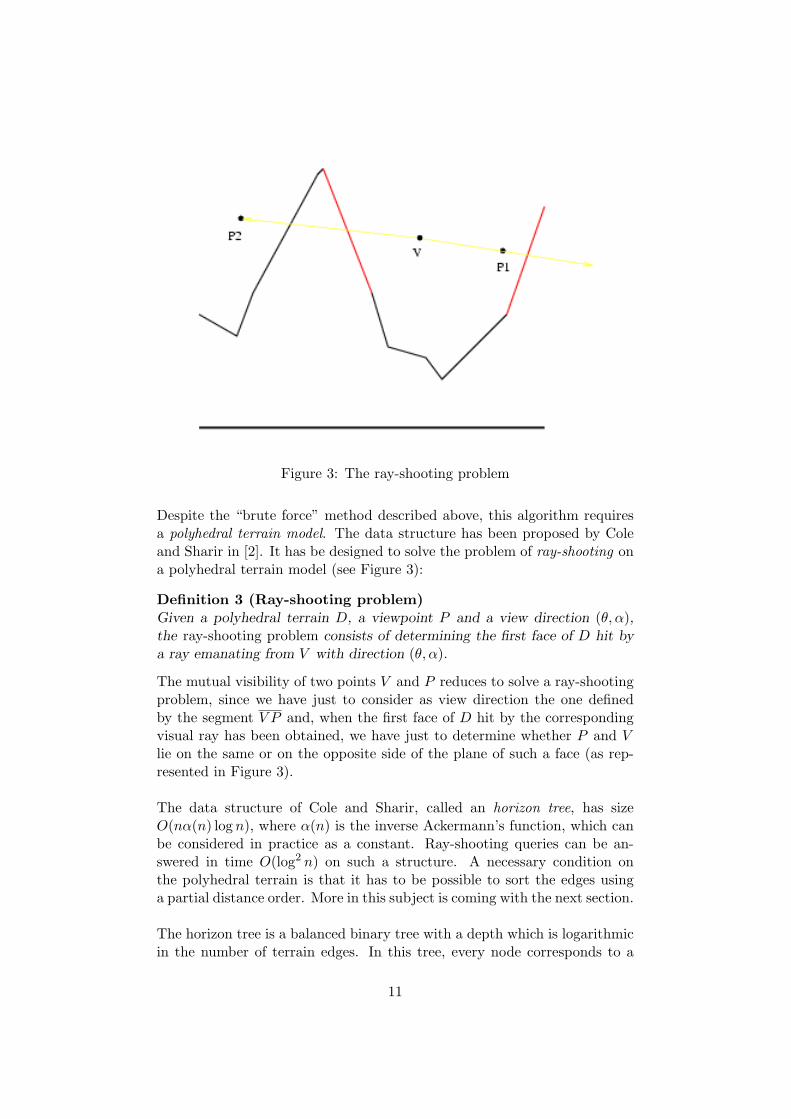
Figure 3: The ray-shooting problem
Despite the “brute force” method described above, this algorithm requiresa polyhedral terrain model. The data structure has been proposed by Coleand Sharir in [2]. It has be designed to solve the problem of ray-shooting ona polyhedral terrain model (see Figure 3):
Definition 3 (Ray-shooting problem)Given a polyhedral terrain D, a viewpoint P and a view direction (θ, α),the ray-shooting problem consists of determining the first face of D hit bya ray emanating from V with direction (θ, α).
The mutual visibility of two points V and P reduces to solve a ray-shootingproblem, since we have just to consider as view direction the one definedby the segment V P and, when the first face of D hit by the correspondingvisual ray has been obtained, we have just to determine whether P and Vlie on the same or on the opposite side of the plane of such a face (as rep-resented in Figure 3).
The data structure of Cole and Sharir, called an horizon tree, has sizeO(nα(n) log n), where α(n) is the inverse Ackermann’s function, which canbe considered in practice as a constant. Ray-shooting queries can be an-swered in time O(log2 n) on such a structure. A necessary condition onthe polyhedral terrain is that it has to be possible to sort the edges usinga partial distance order. More in this subject is coming with the next section.
The horizon tree is a balanced binary tree with a depth which is logarithmicin the number of terrain edges. In this tree, every node corresponds to a
11

subset of edges and stores a partial horizon; the root corresponds to thewhole set of edges of the terrain. Each left child corresponds to the half ofthe edges associated to its parent, that are closest to the viewpoint V , andeach right child corresponds to the remaining half. Every node of the treestores the partial horizon computed on the edges associated with the leftchild of the node.
This horizon tree can be computed in optimal O(nα(n) log n) time, sinceeach partial horizon can be computed by a single application of the algo-rithm of Atallah (see [1]) for determining the horizon of a viewpoint on apolyhedral terrain. A complete description of the algorithm of Atallah isdone in the next section. For further information about the Cole-Sharirdata structure and its use, [4] is a good introduction.
A serious analysis of this method has shown that we can already extractthe needed information (visibility of the candidate points) in the buildingphase of this Cole-Sharir data structure. In other words, we don’t need tosolve a ray-shooting problem for computing the visibility of the candidatepoint. So we don’t need for our purposes the query phase. This fact iseasily understandable, because we don’t need the whole information, likethe face hit by the visual ray, for example. Furthermore, such a structureis appropriate to compute the visibility of points which are not parts of theterrain. This is not a need in our case.
In the next section, we show how to modify this method to extract theneeded information. Furthermore, a complete description of the Atallahalgorithm is done. Last, we present our simplified algorithm.
12

Figure 4: The upper envelope of a set of segments in the plane
4 Description of the Algorithm
In this section, we present our algorithm for computing point visibility on apolyhedral terrain.
4.1 Introduction
As described in the previous section, we use a line visibility algorithm tocompute the horizon with respect to the viewpoint V . During the buildphase of the horizon, it is possible to extract the needed information, i.e. toknow if a point is visible or not.
The computation of the horizon of a viewpoint on a polyhedral terrain re-duces to the computation of the upper envelope of a set of segments in theplane.
Definition 4 (Upper envelope of a set of segments in the plane)Given p segments in the plane, i.e. p linear functions y = fi(x) withi = 1, ..., p, each defined on an interval [ai, bi], the upper envelope of suchsegments is a function y = F (x), defined over the union of the intervals[ai, bi], and such that F (x) = maxi|x∈[ai,bi] fi(x)
Or, in other words, the upper envelope maps any x value in the segmenthaving maximum y value over x, if such a segment exists. Figure 4 shows
13

an example of such an upper envelope of a set of segments.
To reduce the horizon on a polyhedral terrain to the upper envelope ofa set of segments, we can express the edges of the terrain in the sphericalcoordinates system centered at the viewpoint defined in the previous sec-tion. Note that we consider only the two angular coordinates θ and α. Sowe lose information, since two points on the same ray emanating from theviewpoint have the same coordinates. But if the edges are sorted using adistance order, as we will see it later, this information get not lost.
It has been shown in [3] that the complexity of the upper envelope of psegments in the plane is O(pα(p)), and thus, the complexity of the horizonof a polyhedral terrain with n vertices is O(nα(n)). There is different pos-sibilities to compute the envelope of p segments in the plane; either withthe help of a static divide-and-conquer approach leading to a O(pα(p) log p)worst-time case complexity, like the Atallah algorithm ([1]), or with the helpof a dynamic, incremental one, with a complexity of O(p2α(p)). In [4], suchan incremental method is presented, as well as a randomized version, whichhas a time complexity of O(pα(p) log p), too.
4.2 Topological sorting of the edges
As written before, we need to sort the edges using the following partialdistance order
Definition 5 (Distance partial order)Given a plane subdivision Σ and a point O in the plane, an edge e1 of Σ issaid to be before an edge e2 (and e2 behind e1) with respect to O if and onlyif there exists a ray r emanating from O and intersecting both e1 and e2,such that the intersection of r and e1 lies nearer to O than the intersectionof r and e2.
Figure 5 illustrates this definition. We note that this order relation is onlydefined if there is an intersection between the ray and both edges. By usingthe dual graph of the polyhedral terrain, it is possible to sort the set ofedges. This set will be the input of our algorithm.
4.3 A divide-and-conquer approach
The principle of the algorithm is the following: it recursively splits the setof segments into two halves, and pairwise merges the results. Merging twoenvelopes is performed through a sweep-line technique for intersecting twochains of segments.
If the process is done for the farthest edges first and then is coming to
14

Figure 5: Definition of the distance partial order
the nearest, it is possible to know if a point is invisible. As a matter of fact,while merging two horizons, one nearer and one farther, if a vertex of thefarther horizon is under the nearer horizon, then this vertex is invisible, andwe can note this fact. We can remark that we can only know if a point isvisible while the last merge operation, and this if this point is not markedas an invisible one. So, we mark all the points as visible at the begin ofthe horizon computation and following the merging process, we mark theinvisible points.
4.3.1 The divide part
This part is the easily one. At the begin, as written before, the algorithmgets an array of sorted edges, which it will consider as an array of one-piecehorizons. Then, it will merge these horizons two by two to get finally thesearched horizon. This is illustrated in Figure 6.
4.3.2 The conquer part
We present here the “academic” version of this algorithm. The version whichwe have implemented, as well as the changes we have done will be presentedin the next section. To merge two horizons, as in Figure 7, the Atallah algo-rithm uses a sweep-line technique implemented with the help of an event list.The sweep-line algorithm moves an imaginary vertical line r from the left
15

Figure 6: Illustration of the divide phase
Figure 7: Illustration of the conquer phase
16

to the right in such a manner that at each step the resulting upper enveloperestricted to the left half-plane of r has already been computed, while inthe right half-plane, it is still to be determined. The events are representedby the vertices of the two input envelopes, plus the possible intersectionpoints between them. The current status of the sweep-line is represented bythe pair of segments, one each partial envelope, that are intersected by thesweep-line, ordered according to their heights.
There is five possible kinds of events. We list them here, as well as thenecessary update operations needed for the resulting envelope. We use thefollowing colored notation for the illustrations: a blue segment is part of thefarther horizon, while a red one is part of the nearest horizon. The greensegment is the updated part of the resulting envelope. The sweep line is thebrown vertical line, while the last position of this sweep line is the browndashed line.
• If the event is an intersection point of two segments (Figure 8), thenthe current segment in the sweep line status are swapped. The result-ing envelope is updated. In this case, there is no importance in thedistance of the horizons.
Figure 8: Case of an intersection
• If the event is a right endpoint of a segment and if this segment is theactual upper segment (Figure 9), then the interval between the lastevent and the current one is inserted in the resulting envelope.
• If the event is a right endpoint of a segment and if this segment is theactual lower segment (Figure 10), then this segment leaves the status;furthermore, if this segment belongs to the farther horizon as in Figure10, then its right endpoint can be marked as invisible.
• If the event is a left endpoint of a new segment on one of the partialenvelopes, then this segment is inserted in the current status (Figure
17

Figure 9: Case of the right endpoint of the upper segment
Figure 10: Case of the right endpoint of the lower segment
11), in this case as the lower edge. Furthermore, if the new segmentbelongs to the farther partial horizon, as in Figure 11, its left endpointcan be marked as invisible. The intersection between the new pair ofstatus segments is also tested and eventually inserted in the eventqueue.
• If the event is a left endpoint of a new segment on one of the partialenvelopes, then this segment is inserted in the current status, in thiscase as the upper edge (Figure 12). The intersection between the newpair of status segments is tested and eventually inserted in the eventqueue.
18

Figure 11: Case of the left endpoint of a new lower segment
Figure 12: Case of the left endpoint of a new upper segment
19

Figure 13: The two partial horizons are not defined over the same interval
5 Implementation and Integration in the RA3DIO
project
In this section, we present first two problems which were not documented inthe “academic” version, together with the solutions we have chosen to solvethese problems. Then, we give our algorithm in a pseudo-code notation.The integration of this algorithm in a real project has brought some otherdifficulties, which we present next. Finally, we make a brief presentation ofthe implementation, together with some comments when needed.
5.1 Problems and solutions
The algorithm of Atallah, as presented in [4], is designed for “friendly” par-tial horizons, which begin and end both at the same points and continuous.This is naturally not the case in a real-world application. A first problemwas to find an acceptable solution in the cases where a partial horizon isnot defined, as illustrated in Figure 13. The solution we chose is the follow-ing: everywhere where the horizon is not defined, we insert an horizontalhole-edge, with an α set to an impossible value, −2 in our implementa-tion. So the horizons are all defined over the interval [0, 2π], and holes aretreated as they were horizons parts. This solution is illustrated in Figure 14.
Another problem which happens in a real-world application is the possi-
20

Figure 14: The “hole-edges” solution
bility that the partial horizons are not continuous, in the sense that theright endpoint of a segment and the left endpoint of the next segment havenot the same α-value, as illustrated in Figure 15. Or, in other words, wehave to keep our algorithm robust even if there is jumps in the partial hori-zons. The problem is the situation where an edge of the other partial horizonpasses through this kind of jump. In this case, we have sometimes to inserta new part in the resulting envelope and to modify the internal status of thesweep line.
5.2 The final version of our algorithm
We give here the pseudo-code (in a C++-like notation) version of our algo-rithm.
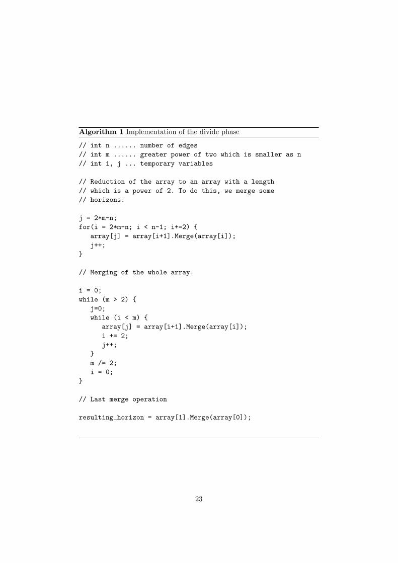
5.2.1 Implementation of the divide phase
For efficiency purposes, we have chosen to implement the recursion in aniterative way. Since we cannot expect that the number of edges is a powerof two, we merge first a part of the array of edges, which are topologicallysorted, to reduce the size to the greatest power of two which is smaller thanthis number of edges. Then, we can use a simple loop to merge the resultinghorizons in a tree-like structure. This is illustrated in Algorithm 1. Werecall that we have to do the merge operations for the farther horizons first
21

Figure 15: The jump-problem
and at last for the nearest ones, so we don’t forgive invisible vertices. Thefarthest edge is stored in the first case of the array, while the nearest one isstored in the last case.
5.2.2 Implementation of the conquer phase
The conquer phase is by far the most complex operation in the algorithm.This procedure first builds the event list, and then processes the events, up-dating the resulting envelope when needed. It is naturally in this procedurethat the invisibility of some vertices is determined. The pseudo-code versionof this procedure is in Algorithm 2 and the end is in Algorithm 3.
22
Algorithm 1 Implementation of the divide phase
// int n ...... number of edges// int m ...... greater power of two which is smaller as n// int i, j ... temporary variables
// Reduction of the array to an array with a length// which is a power of 2. To do this, we merge some// horizons.
j = 2*m-n;for(i = 2*m-n; i < n-1; i+=2) {
array[j] = array[i+1].Merge(array[i]);j++;
}
// Merging of the whole array.
i = 0;while (m > 2) {
j=0;while (i < m) {
array[j] = array[i+1].Merge(array[i]);i += 2;j++;
}m /= 2;i = 0;
}
// Last merge operation
resulting_horizon = array[1].Merge(array[0]);
23

Algorithm 2 Implementation of the conquer phase (1)
// Building of the event list for the farther// partial horizon.
forall(segment [a, b] in farHorizon) {insert a in eventList marked as LEFT_ENDOINT;insert b in eventList marked as RIGHT_ENDPOINT;
}forall(segment [a, b] in nearHorizon) {
insert a in eventList marked as LEFT_ENDOINT;insert b in eventList marked as RIGHT_ENDPOINT;
}status.inf = UNDEFINED;status.sup = UNDEFINED;lastEvent = 0.0;
// Main loop
while(eventList.notEmpty()) {currentEvent = eventList.nextEvent();switch(e.eventType()) {
case INTERSECTION:insert [lastEvent, currentEvent] in
the resulting envelope with labelstatus.sup;
lastEvent = currentEvent;Swap(status.inf, status.sup);break;
case RIGHT_ENDPOINT:if(currentEvent right endpoint
of status.sup) {insert [lastEvent, currentEvent] in
the resulting envelope with labelstatus.sup;
lastEvent = currentEvent;status.sup = status.inf;status.inf = UNDEFINED;
} else {
24

Algorithm 3 Implementation of the conquer phase (2)
if (status.inf belongs to farHorizon) {mark right endpoint of status.inf
as invisible;}status.inf = UNDEFINED;
} // end of elsebreak;
case LEFT_ENDPOINT:snew = segment whose left endpoint is
currentEvent;if (snew over status.sup) {
status.inf = status.sup;status.sup = snew;if (jump_situation) {
insert missing part in the resultingenvelope;
} else {if (status.inf belongs to farHorizon) {
mark left endpoint of status.infas invisible;
}status.inf = snew;
}if (status.sup and status.inf intersect) {
(x, y) = intersection point;insert x in eventList, marked asINTERSECTION;
}break;
} // end of switch statement} // end of while
25

Figure 16: The subdivision of the terrain in patches
5.3 The integration in a patch environment
In the RA3DIO project, the terrain is subdivided in small pieces, which areeasier to load and to display than the whole terrain. Such a small piece ofterrain is called a patch. Each patch is a square and has about 3000 edgesin the actual configuration. We can use the presented algorithm to computethe horizon line and for determining the (in-)visibility of the points, but ifwe have to compute the visibility of points which are not in the same patchas the viewpoint, the task becomes more difficult.
The situation is illustrated in Figure 16. For example, to compute thehorizon line of the patch number 2, we have first to compute the internalhorizon line of the patch, and then to merge this horizon line with the por-tion of the horizon of the patch number 1 delimited by the α value, or, inother words, with the north side of the central patch.
In a more complicated manner, the computation of the visibility of thepoints in the patch number 8 needs the following operations: first we haveto compute the internal horizon line and then to merge this horizon withthe β portion of patch number 5 and with the γ portion of patch number 4.
26

Figure 17: The processing order in a patches environment
Thus, for computing the visibility of the points in a 3x3- or a 5x5-gridof patches, they must be preprocessed in a way, such that the horizons areavailable when needed. This gives us the processing order illustrated in Fig-ure 17. To merge the southern part of the horizon line of patch number5 with the eastern one of patch number 4, we have just to append thesetwo horizons. But for computing the horizon line of patch number 6, theoperation is more complicated, because the patch is “cut” by the x-axis. So,in this kind of situation, we have to treat these horizons in a special way.These two situations are summarized in Figure 18.
5.4 Description of the classes and methods
In this part, we present briefly the three new classes which were inserted inthe RA3DIO project. The algorithm has been implemented in C++. TheLEDA library (see [5] for a description) has been employed for the com-mon data structures. During the development time, [6] has been used as areference book.
27

Figure 18: Handling of normal horizons and “cut” horizons
5.4.1 The CEventItem class
The CEventItem class defines the properties of the events which are usedduring the merge procedure. The main goal of this class is to store informa-tion needed by the algorithm for its (imaginary) sweep line. The methodsare all procedures which permit to read and to set the class variables.
5.4.2 The CHorizonItem class
An horizon is in fact a list of CHorizonItems, which can be viewed as thesegments in an horizon. Again, the methods are all procedures which permitto set and to read the class variables.
5.4.3 The CHorizon class
This class is by far the most complicated and the most interesting one. Itmodels the concept of an horizon line. The CHorizon class is a subtype ofa LEDA double-linked list. It has the following methods:
• CHorizon(CHorizonItem& horizonItem) is a constructor used to buildan horizon object with a single horizonItem object. It is used to
28
transform a set of edges in a list of one-piece horizons, inserting thenecessary holes.
• CHorizon(leda list<CHorizonItem>& array, CTransmitter* tx,CPatch *patch, CHorizon& horizon = CHorizon()) is a construc-tor used to build a new horizon. It computes the internal horizon line,and if needed, merges this new horizon line with the one stored in theinput variable horizon. The implementation of the divide phase isdone in this method.
• CHorizon Merge(CHorizon& horizon, double leftLimit, doublerightLimit, bool last) is the conquer part of the algorithm. Forefficiency reasons, Merge() takes an interval as input and merges thetwo partial horizons only between these two values, which considerablyreduces the number of events in the most number of the cases.
• bool Over(const leda segment sinf, const leda segment ssup,double x) const decides whether an edge is over another, in an hori-zon. Note that the decision is defined when the two edges are holes,too.
5.4.4 The PatchPreprocess() method
void CWaveModelPointVis::PatchPreprocess(CTransmitter* tx,CPatch* patch) is the method called by RA3DIO when the user puts aviewpoint on the terrain. It is called in the good order, as defined in Figure17. The following operations are done: it creates first a directed copy ofthe (undirected) dual graph of the polyhedral terrain, then the topologicalsorting of the triangle edges is done, it computes the visibility of all thepoints, marks the invisible ones and merges the patches horizons, whenneeded. Another method, while displaying the terrain, will test for eachvertex if it is visible or not.
29
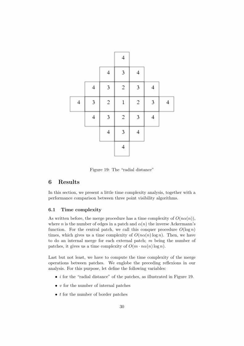
Figure 19: The “radial distance”
6 Results
In this section, we present a little time complexity analysis, together with aperformance comparison between three point visibility algorithms.
6.1 Time complexity
As written before, the merge procedure has a time complexity of O(nα(n)),where n is the number of edges in a patch and α(n) the inverse Ackermann’sfunction. For the central patch, we call this conquer procedure O(log n)times, which gives us a time complexity of O(nα(n) log n). Then, we haveto do an internal merge for each external patch; m being the number ofpatches, it gives us a time complexity of O(m · nα(n) log n).
Last but not least, we have to compute the time complexity of the mergeoperations between patches. We englobe the preceding reflexions in ouranalysis. For this purpose, let define the following variables:
• i for the “radial distance” of the patches, as illustrated in Figure 19.
• v for the number of internal patches
• t for the number of border patches
30

• l for the maximal length of the horizon
• c for the average length of the horizon per border patch
• H for the time needed to compute the horizon
We have following values for these different variables:
i u v t l c H
1 1 1 1 nα(n) 1 1
2 4 1 5 5nα(5n) 5/4 4 · 1 = 4
3 8 5 13 13nα(13n) 13/8 4 · 5/4 + 8 · 5/4 = 15
4 12 13 25 25nα(25n) 25/12 4 · 13/8 + 16 · 13/8 = 3212
5 16 25 41 41nα(41n) 41/16 4 · 25/12 + 24 · 25/12 = 5813
We have the following equalities between these variables:
ui = 4(i− 1)
vi = 1 +i−1∑j=1
uj = 2i2 − 6i + 5
ti = ui + vi = 2i2 − 2i + 1
Hi = uinα(n) log n+4ci−1 +(ui− 4) · 2 · ci−1 = uinα(n) log n+2ci−1(ui− 2)
We can approximate Hi as follows:
Hi = O(i)nα(n) log n + 2O(i− 1)nα(O(i− 1)2n)(4i− 6)
which is finallyO(i)nα(n) log n + 2O(i2)nα(i2n)
To get the final time complexity estimation, we have to sum these Hi’s:
m∑i=2
(nα(n) log n + O(i) · n · α(i2n)
)+ nα(n) log n
which gives us:O(mnα(n) log n + m2nα(m2n))
We can remark that when the number of patches tends to the number ofedges pro patches, then our algorithm is not very interesting. This is not thecase in the reality, the number of patches being relatively small comparedto the number of edges in a patch.
31

6.2 Comparison between the three algorithms
We make now a comparison between the three algorithms presented in thissemester thesis. The two first are easily implementable and are available inthe RA3DIO project. We recall that the first one, which use a “brute-force”strategy, has a complexity of O(m ·n2). The second one, which uses specificproperties of polyhedral terrains, has a time complexity of O(m ·n3/2). Thefollowing table summarize time measures (in seconds) for the computationof point visibility for different numbers of patches. The number of edges perpatch n is equal to about 3000.
# patches O(m · n2) O(m · n√
n) O(mnα(n) log n + m2nα(m2n))1 0.5 0.2 2.89 12.5 6.2 24.5
25 71.6 31.7 52.249 179.8 71.9 108.981 353.9 130.6 196.9
The first remark we can do is that the algorithm with a quadratic complex-ity becomes fast the slowest one, and that it is not practical. Secondly, it isclear that the second algorithm is faster than the third. We can understandthis fact as follows: the implementation of the second one is very simple andthus the constant term is quite small, while our algorithm is quite compli-cated. Therefore, the little number of edges per patch handicaps the relativeperformance of the theoretical faster one.
Now, it is possible to improve its performances by many ways. First of all,the divide-and-conquer strategy could allow a parallelization of the com-putation of the horizon line. Then, it is always possible to improve theperformances by optimizing the code. But it is quite time consuming !
32

7 Conclusion
It is now time to conclude this semester thesis. We have developed andimplemented a (theoretical) fast algorithm for computing point visibility ona polyhedral terrain. This algorithm has been integrated in the RA3DIOproject, which means that a lot of not documented problems have requestedrobust solutions.
However, our algorithm is not faster than a more trivial one, which is betterfor the parameters used in a typical RA3DIO utilization. This fact illus-trates well the differences between a theoretical proposition and a practicalapplication of such a “fast” algorithm.
In a more personal way, I have enjoyed this work a lot, because it hasbrought to me experience in programming in C++, as well in managing arelative big implementation. Furthermore, it is quite interesting to workin the border of the theory and the practice. Finally, I will keep excellentmemories of the house, of the little desk under the roof and of the life in alittle team.
33

References
[1] M. Atallah. Dynamic computational geometry. In Proc. 24th Symposiumon Foundations of Computer Science, pages 92–99. IEEE Computer So-ciety, Baltimora, 1983.
[2] Richard Cole and Micha Sharir. Visibility problems for polyhedral ter-rains. Journal of Symbolic Computation, 7(1):11–30, January 1989.
[3] H. Edelsbrunner. The upper envelope of piecewise linear functions: tightbounds on the number of faces. Discrete and Computational Geometry,4:337–343, 1989.
[4] L. De Floriani and P. Magillo. Visibility algorithms on triangulated ter-rain models. International Journal of Geographic Information Systems,8(1):13–41, 1994.
[5] Leda homepage : http://www.mpi-sb.mpg.de/LEDA.
[6] Stanley B. Lippman and Josee Lajoie. C++ Primer, 3rd Edition. Addison-Wesley, 1998.
[7] The project homepage : http://www.ra3dio.ethz.ch.
34


