b

UCRL-ID-lZl742 .. .

Implementation of a Random Displacement Method (RDM) in the ADPIC

Model Framework

Donald L. Ermak John S. Nasstrom Allan G. Taylor

June 1995

DISCLAIMER

This document was prepared as an account of work sponsored by an agency of the United States Government. Neither the United States Government nor the University of California nor any of their employees, makes any warranty, express or implied, or assumes any legal liability or responsibility for the accuracy, completeness, or usefulness of any information, apparatus, product, or process disclosed, or represents that its use would not infringe privately owned rights. Reference herein to any specific commercial products, process, or service by trade name, trademark, manufacturer, or otherwise, does not necessarily constitute or imply its endorsement, recommendation, or favoring by the United States Government or the University of California. The views and opinions of authors expressed herein do not necessarily state or reflect those of the United States Government or the University of California, and shall not be used for advertising or product endorsement purposes.

This report has been reproduced directly from the best available copy.

Available to DOE and DOE contractors from the Oftice of Scientific and Technical information

P.O. Box 62, Oak Ridge, TN 37831 Prices available from (615) 576-8401, FITS 626-8401

Available to the public from the National Technid Information Service

US. Department of Commerce 5285 Port Royal Rd.,

Springfllld, VA 22161

DISCLAIMER

Portions of this document may be illegible in electronic image products. Images are produced from the best available original document.

Contents

Page

1. Introduction 1 .............................................................................................................

2. Euleian and Lagrangian equations ........................................................................ 1

3. N u m e n d solution ................................................................................................... 2

3.1 Finite difference equations ............................................................................. 2

3.2 Time step 3

4. Validztion of the RDM versus analytic solutions ................................................... 4

5. Acknowledgments .................................................................................................... 9

6. References ................................................................................................................ 9

Appendix I: RDM implementation. ............................................................................ 10

.........................................................................................................

Appendix II: FORTRAN Namefist input parameters ............................................... 14

1. Introduction

The objective of this work was to implement a 3-D Lagrangian stochastic (also called random walk or Monte Carlo) diffusion method in the framework of the operational ADPIC (Atmospheric Diffusion Particle-In-Cell) code (Lange, 1989; Taylor et al., 1993). The Random Displacement Method, RDM, presented here and implemented in the ADPIC code, calculates atmospheric dispersion in a purely Lagrangian, grid-independent manner. Some of the benefits of this approach compared to the previously-used "particle- in-cell, gradient diffusion" method are (a) a sub-grid diffusion approximation is no longer needed, (b) numerical accuracy of the diffusion calculation is improved because particle displacement does not depend on the resolution of the Eulerian grid used to calculate species concentration, and (c) adaptation to other grid structures for the input wind field does not affect the diffusion calculation. In addition, the RDM incorporates a unique and accurate treatment of particle interaction with the surface.

2. Eulerian and Lagrangian equations

The Random Displacement Method (RDM) is based, as is the particle-in-cell, gradient diffusion method, upon the conservation of species principal expressed in the form of the 3-D, incompressible, Eulerian advection-diffusion equation:

where c is the mean air concentration of the species; ii, V , and Fare the mean wind components in the x, y, and z directions, respectively; t is time; and Kk Ky, and K, are the eddy diffusivities for the three coordinate directions (the eddy diffusivity tensor is assumed to be diagonal).

The RDM uses stochastic differential equations that describe the same process as the advection-diffusion equation (l), but in a Lagrangian instead of an Eulerian framework (Boughton et al., 1987; Ermak, 1992; Rodean et al., 1992). The stochastic differential equations for the displacement of an idealized fluid element in the three coordinate directions are

dx = Edt + ( 2 K X ) X d w , ,

dy = Fdt+ (2Ky)KdW,, and

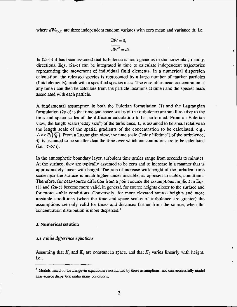
where dw,,, are three independent random variates with zero mean and variance dt, i.e., - dW=o,

dW2 = dt. -

In (2a-b) it has been assumed that turbulence is homogeneous in the horizontal, x and y, directions. Eqs. (2a-c) can be integrated in time to calculate independent trajectories representing the movement of individual fluid elements. In a numerical dispersion calculation, the released species is represented by a large number of marker particles (fluid elements), each with a specified species mass. The ensemble-mean concentration at any time t can then be calculate from the particle locations at time t and the species mass associated with each particle.

A fundamental assumption in both the Eulerian formulation (1) and the Lagrangian formulation (2a-c) is that time and space scales of the turbulence are small relative to the time and space scales of the diffusion calculation to be performed. From an Eulerian view, the length scale ("eddy size") of the turbulence, I., is assumed to be small relative to the length scale of the spatial gradients of the concentration to be calculated, e.g., L << C,/(g). From a Lagrangian view, the time scale ("eddy lifetime") of the turbulence, z, is assumed to be smaller than the time over which concentrations are to be calculated (i.e., z cc t).

In the atmospheric boundary layer, turbulent time scales range from seconds to minutes. At the surface, they are typically assumed to be zero and to increase in a manner that is approximately linear with height. The rate of increase with height of the turbulent time scale near the surface is much higher under unstable, as opposed to stable, conditions. Therefore, for near-source diffusion from a point source the assumptions implicit in Eqs. (1) and (2a-c) become more valid, in general, for source heights closer to the surface and for more stable conditions. Conversely, for more elevated source heights and more unstable conditions (when the time and space scales of turbulence are greater) the assumptions are only valid for times and distances farther from the source, when the concentration distribution is more dispersed.*

3. Numerical solution

3.1 Finite difSerence equations

Assuming that Kx and Ky are constant in space, and that K, varies linearly with height, i.e.,

* Models based on the Langevin equation are not limited by these assumptions, and can successfully model near-source dispersion under many conditions.

2

a numerical solution of Eqs. (2a-c) can be constructed using the difference equations (Ermak, 1992):

Axi = EAti + [2KXiAtilg 6,- ( 4 4

(4b) K Ayi = FAti + [2 KyiAti] tYi

Azj = ZAtj + 2 Atj + 2KzjAtj + 2 Atj2 tZj (: )i [ (2 1% where, for example, in the vertical direction,

dzj = Z(ti,l) - z&), K,i = K, (Z i 9 ti 1,

( %)i = !& r=zj ’

Ati = ti+l - ti , and - 6= = a random number with zero mean (6 = 0) - and variance of one ( t2 = 1).

The second-order term in (k), (&C/dz)2At2, is unique to our RDM. This term includes the effect of the linear variation of K during the finite time step, At, on the displacement variance, and is especially important close to the ground where K, approaches zero in similarity theory parameterizations (Nasstrom (1995) described the K parameterization options available for the RDM). Particle trajectories can be numerically calculated by successively using (4a-e) and incrementing the particle position using, for example,

Details on the implementation of (4-5) are given in Appendix A.

3.2 Time step In the ADPIC code, a gridded wind field is used for the mean wind components, E, ij, and iij in (4a-e). Consequently, the time step used in the numerical solution is

3

restricted to prevent a particle from moving more than a single mean wind grid cell in any time step due to mean wind advection plus diffusion. Furthermore, for accurate time integration of concentration in the concentration grid, the time step is also restricted to prevent any particle from moving through more than a single concentration grid cell in any time step (this results in conservatively small time steps when the concentration distributions span many sampling grid cells).

In the RDM, the time step is determined separately for each particle. The eddy diffusivity and the spatial derivative of the vertical eddy diffusivity are evaluated analytically at the particle position at each time step. The particle time steps for all particles are forced to synchronize at necessary times, such as when meteorological parameters change, source parameters change, wind input data changes, particle concentrations are to be saved, status messages are to be written, or graphics output is to be written.

4. Validation of RDM versus analytic solutions To validate the implementation of the RDM, calculations were performed and compared to three types of exact analytic solutions of the advection-diffusion equation (1). First, a successful no-diffusion, advection-only comparison was made to confirm that a Gaussian concentration distribution is accurately advected through the concentration sampling grid and that the time-integrated concentration is accurately calculated. Second, a series of point source releases at various elevations under uniform mean wind speed and constant K,, Ky, and Kz conditions were simulated. Again, the RDM results were in excellent agreement with the analytic solutions which are time-d endent Gaussian concentration distributions with standard deviations o, ,~ ,~ = (2Kx,y,zt) . Finally, a more complex case of inhomogeneous turbulence was simulated and compared with the analytic solution. Details of this latter comparison and its results follow.

E)

This case study was chosen to test the RDM under inhomogeneous turbulence conditions that included significant interaction of the dispersing plume with the lower boundary. The release scenario involved a continuous source at the ground surface,

with a unit source rate,

The eddy diffusivities and mean wind speed were chosen to be representative of a neutral surface layer, as follows:

ii = 5 m/s,

q ( x ) = 0.15 x 0.92 m, and

Kx = 0.

Ky was calculated using the relationship

The grid used for calculating the concentration from the particle positions was nested in the horizontal with a resolution of 3.125 m in the innermost (fourth) nested grid near the source and 50 m in the outermost grid. The vertical resolution was 5 m. The domain was 2 km in the horizontal and 210 m in the vertical.

The RDM-calculated mean concentrations were compared to concentrations obtained by using the following analytic solution to the advection-diffusion equation taken from Brown et al. (1993):

This solution for the mean concentration (e.g., g/m3) assumes (a) a continuous point source with source strength Q, (e.g., in g/s); (b) the vertical eddy diffusivity is a linear function of height, K, ( z ) = K,z ; (c) a Gaussian horizontal concentration distribution with standard deviation, oy(x); (d) no alongwind diffusion, Le., K, = 0; (e) the mean wind speed, ii , is constant with height; (f) zero vertical mass flux at the ground surface; and (g) the source location is at coordinates x= 0, y = 0, and z = 0.

Figs. 1-3 show results comparing concentrations calculated using the RDM to those calculated by the analytic solution (7). Figs. 1 and 2 show excellent agreement between the contours of concentration from the analytical solution and the RDM, respectively, at a height of 10 m for a horizontal domain extending 1.8 km downwind of the source. The RDM contours in Fig. 2 are not as smooth as those in Fig. 1 due to the different concentration grid resolutions within different nested grids in the RDM computational domain. Fig. 3 also shows excellent agreement in a plot of concentration calculated by the analytic solution (solid line) and by the RDM (individual points) versus height at a downwind distance of 1.5 km along the centerline of the plume. Note the highly non- Gaussian shape of the vertical concentration profile. This exponential behavior of the concentration profile is primarily due to the linear variation with height of the vertical eddy diffusivity near the ground.

5

Concentration ( g / m 3 ) at z=10. m 1

. . . . . . . . . . . . . . . . . . . . . . . . . ( 1 .

0 0.25 0.5 0.75 1 1.25 1.5 1 .I5

0 .75

0.5

0.25

Y ( W O

-0 .25

-0 .5

-0 .75

Figure 1. Contours of mean concentration (g/m3) calculated by the analytic solution given in E%+ (7) with assumptions (6a-fj at a height of 10 m in a horizontal domain of 1.8 x 1.8 km. Contour levels are 3 x (innermost), 1.5 x lW5, 3 x le6, and 1 x 1W6 g/m3 (outermost), as in Fig. 2. The units of the x and y axes are kilometers from the source location. Contours were drawn using a uniform 320 by 320 dimension horizontal array of concenuation values.

6

c

1

0

0

0

0

0

-0

.O

-0

-0

-1

Pld Generatbn Tlme 1 WAN95 19:18:00 UTC

Contour Integrated Type at 10.0 meters 1 01FE894 00:06:00 to 01FEB94 00:12:00 UTC

sigy=0.15'xA0.92, Kx=O.

Continuous, Sfc release

> 1.50e-05 glm3 0.201 577 sq km

> 3.008-06 glm3 0.580571 sq km

> 1.00e-06 glm3 0.724833 sq km

~

0.0 0 2 0.4 0.6 0.8 1 .o 1.2 1.4 1.6

kilometers

0.0 0.2 0.4 0.6 0.8 1 .o

Figure 2. Contours of mean concentration (g/m3) calculated by the RDM with assumptions (6a-f) at a height of 10 m. Contour levels are 3 x lW5 (innermost), 1.5 x 3 x 10-6, and 1 x 10-6 g/m3 (outermost), as in Fig. 1. The units of the x and y axes are kilometers from the source location. Contours were drawn using concentration values from four nested grids with a resolution of 3.125 m in the innermost grid near the souxe and 50 m in the outermost grid. Note the domain used to plot these contours is slightly larger than in Fig. 1, but the scale is the same.

7

Concentration vs. height at x=1.5 km, y=O. km

100

80

60

z (m)

40

20

J 2.5 5 7.5 10 12.5 15 17.5

Mean concentration (g/m3) x 1.E-6

Analytical solution 1-,/ Figure 3. Mean concentration (g/m3) versus height (m) calculated by the RDM (points) and the analytic solution (solid line) given by Eq. (7) with assumptions (6a-f) at a downwind distance, x, of 1.5 km at the centerline (y = 0) of the plume. RDM concentrations represent grid-cell volume averages and analytic concentration values were volume-averaged in a similar manner for comparison.

8

6. References Boughton, B.A., J.M. Delaurentis, and W.E. Dunn (1987) A stochastic model of particle

dispersion in the atmosphere, Boundary-Layer Meteor., 40,147- 163. Brown, M.J., S.P. Arya, and W.H. Snyder (1993) Vertical dispersion from surface and

elevated releases: an investigation of a non-Gaussian plume model, 3. Appl. Meteor.,

Em&, D.L. (1 992) Dense-Gas Dispersion Advection-Diffusion Model. Proceedings JANNAF Safety and Environmental Protection Subcommittee meeting, Aug. 10- 14, 1992, Chemical Propulsion Information Agency, CPIA Pub. 588, pp. 215-224. Also, Lawrence Livermore National Laboratory, Livermore, CA, publication UCRL-JC- 109697.

Lange, R. (1989) Transferability of a Three-Dimensional Air Quality Model between Two Different Sites in Complex Terrain, J. Appl. Meteorol., 28,7, pp. 665-679

Nasstrom, J.S. (1995) Turbulence parameterizations for the RDM version of ADPIC, UCRL-ID- 120965, Lawrence Livermore National Lab., Livermore, California.

Rodean, H.C., R. Lange, J.S. Nasstrom, and V.P. Gavrilov (1992) Comparison of two stochastic models of scalar diffusion in turbulent flow. Preprint, Tenth Symposium on Turbulence and Diffusion, 29 Sept.-2 Oct. 1992, Portland, OR. Published by the American Meteorological Society, Boston, MA.

Taylor et al. (eds.), (1993) User's Guide to the MATHEW/ADPIC Models, UCRL-MA- 103581 Rev. 2.0, LLNL, Livermore, CA, .

32,490-505.

J

5. Acknowledgments We would like to thank H.C. Rodean, E. Nalund, R. Lange, and L.A. Lawson for their help with earlier versions of the random displacement method. This work was performed under the auspices of the U.S. Department of Energy by Lawrence Livermore National Laboratory under contract number W-7405-Eng-48.

Appendix I: RDM implementation

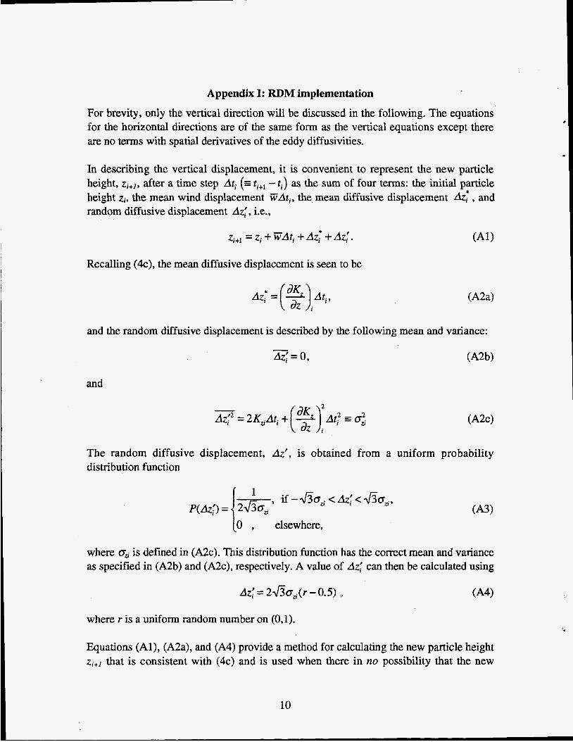
For brevity, only the vertical direction will be discussed in the following. The equations for the horizontal directions are of the same form as the vertical equations except there are no terms with spatial derivatives of the eddy diffusivities.

In describing the vertical displacement, it is convenient to represent the new particle height, z ~ + ~ , after a time step Ati ( E ti+l - ti) as the sum of four terms: the initial particle height zi, the mean wind displacement ZAti, the mean diffusive displacement Az: , and random diffusive displacement Az,’ , i.e.,

Recalling (k), the mean diffusive displacement is seen to be

= ( %)Ati ’

and the random diffusive displacement is described by the following mean and variance:

and

The random diffusive displacement, Az‘, is obtained from a uniform probability distribution function

elsewhere,

where a, is defined in (A2c). This distribution function has the correct mean and variance as specified in (A2b) and (A~c) , respectively. A value of Azl can then be calculated using

Az,’ = 2&,(r - 0.5)

where r is a uniform random number on (0,l).

Equations (Al), (A2a), and (A4) provide a method for calculating the new particle height zi+l that is consistent with (4c) and is used when there in no possibility that the new

10

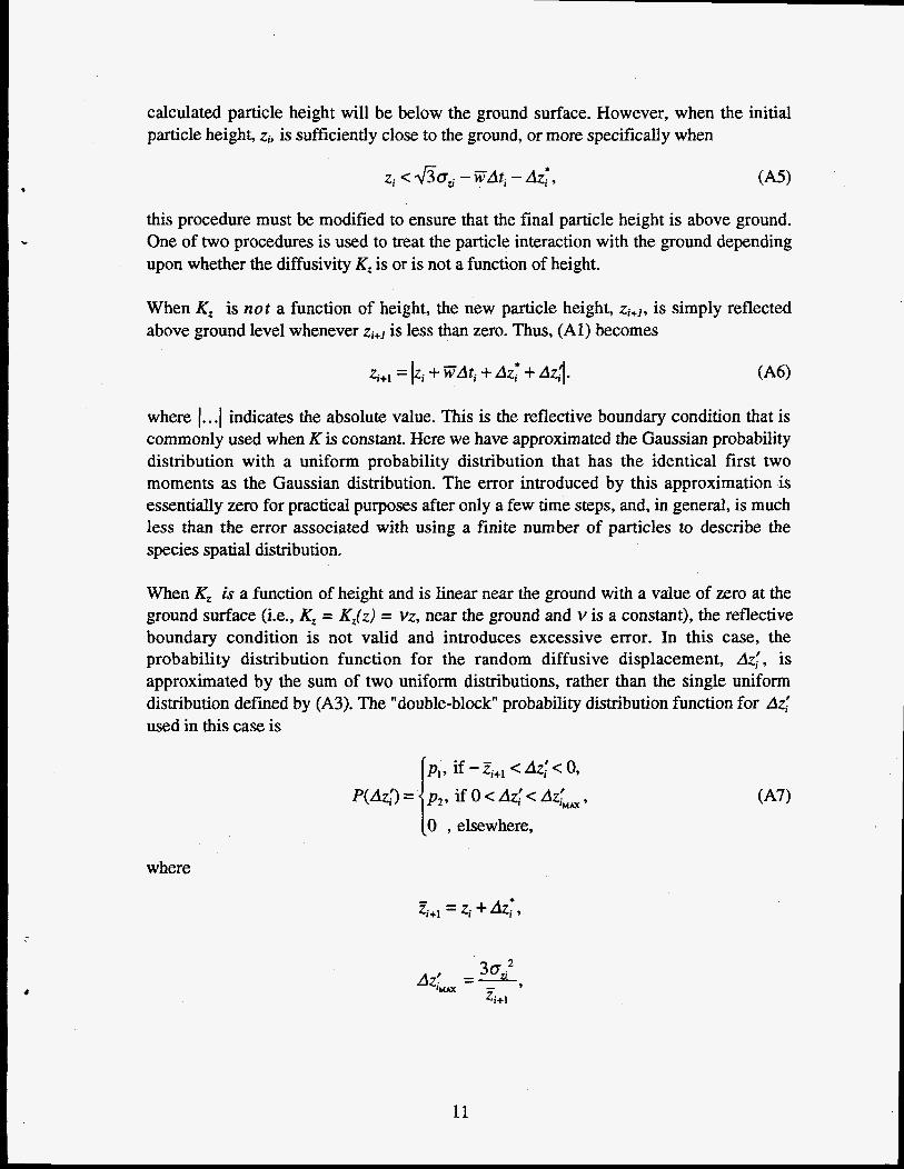
calculated particle height will be below the ground surface. However, when the initial particle height, zi, is sufficiently close to the ground, or more specifically when

this procedure must be modified to ensure that the final particle height is above ground. One of two procedures is used to treat the particle interaction with the ground depending upon whether the diffusivity K, is or is not a function of height.

When K, is not a function of height, the new particle height, z ~ + ~ , is simply reflected above ground level whenever zi+l is less than zero. Thus, (Al) becomes

where I...I indicates the absolute value. This is the reflective boundary condition that is commonly used when K is constant. Here we have approximated the Gaussian probability distribution with a uniform probability distribution that has the identical first two moments as the Gaussian distribution. The error introduced by this approximation is essentially zero for practical purposes after only a few time steps, and, in general, is much less than the error associated with using a finite number of particles to describe the species spatial distribution.

When K, is a function of height and is linear near the ground with a value of zero at the ground surface (i.e., K, = K,(z) = vz, near the ground and v is a constant), the reflective boundary condition is not valid and introduces excessive error. In this case, the probability distribution function for the random diffusive displacement, Az,!, is approximated by the sum of two uniform distributions, rather than the single uniform distribution defined by (A3). The “double-block” probability distribution function for Az,’ used in this case is

p l , if -Zi+l < Az,’< 0,

0 , elsewhere, p2, if 0 < Az,’ < AZ;, ,

where

11

The random diffusive displacement, Azl , can then be calculated as follows:

where ri is a uniform random number on (0,l).

This approach to calculating the total diffusive displacement (Azi* + Az,') when the diffusivity is a function of height and linear near the ground has two unique features. First, it yields the exact values for the first and second moments of the total diffusive displacement and, second, it provides a value for the new particle position, z ~ + ~ , in the absence of the mean wind Z, that is always greater than zero. Consequently, reflection at the ground surface is not needed to correct an unacceptable total diffusive displacement that puts the particle below the ground surface.

Finally, the new particle position, z ; + ~ , is then calculated by adding in the old particle position, z;, and the mean wind displacement, VAt;, using an equation of the same form as (A6), namely

z ; , ~ =lzi+ VAti+Az,* +Azd ,

where the mean diffusive displacement, Az;, is calculated from (A2a), as before, and the random diffusive displacement, Az,', is calculated from (AS) rather than (A4). The reflection condition implied by the absolute value sign in (A9) is applied to correct minor error, if any, in the mean wind displacement, i7Ati, that places the particle below the ground surface.

The above discussion of the RDM calculation of the vertical displacement and its treatment of the interaction with the ground surface basically applies when the terrain is flat. In general, a particle can end up below the ground surface as the result of minor errors in both the vertical and horizontal displacements as the code attempts to advect and diffuse the particle over and/or around the "step" representation of terrain in ADPIC.

12

f

The general procedure within ADPIC to ensure that particles remain above the ground surface is as follows: (1) If the terrain elevation of the new particle (x,y) location is less than or equal to the terrain elevation before the displacement, then the particle is simply reflected vertically. Otherwise, the particle height is shifted up one grid level at a time (up to a specified maximum number of shifts) in an attempt to place the particle above terrain; (2) If step (1) fails to place the particle above terrain, then the code returns the particle to its initial displacement height below the terrain and attempts to move the particle horizontally around the terrain; and (3) If step (2) fails to place the particle above terrain, then the particle is returned to its original location and no displacement of the particle occurs.

13

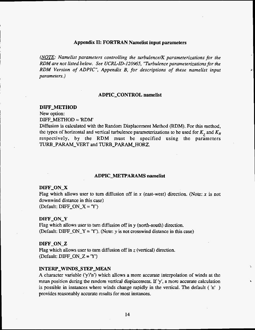
Appendix II: FORTRAN Namelist input parameters

(NOTE: Namelist parameters controlling the turbulence/K parameterizations for the RDM are not listed below. See UCRL-ID-I2096.5, "Turbulence parameterizations for the

parameters.)

r

RDM Version of ADPIC", Appendix B, for descriptions of these namelist input 5

ADPIC-CONTROL namelist

DIFF-METHOD New option: DIFF-METHOD = 'RDM' Diffusion is calculated with the Random Displacement Method (RDM). For this method, the types of horizontal and vertical turbulence parameterizations to be used for Kz and KH respectively, by the RDM must be specified using the parameters TURB-PARAM-VERT and TURB-PARAM-HORZ.

ADPIC-METPARAMS namelist

DIFF-ON-X Flag which allows user to turn diffusion off in x (east-west) direction. (Note: x is not downwind distance in this case) (Default: DIFF-ON-X = 'Y')

DIFF-ONY Flag which allows user to turn diffusion off in y (north-south) direction. (Default: DIFF-ONY = 'Y'). (Note: y is not crosswind distance in this case)

DIF'F-ON-Z Flag which allows user to turn diffusion off in z (vertical) direction. (Default: DIFF-ON-Z = 'Y')

INTERP-WINDS-STEP-MEAN A character variable ('y'h') which allows a more accurate interpolation of winds at the mean position during the random vertical displacement. If 'y', a more accurate calculation is possible in instances where winds change rapidly in the vertical. The default ( 'n' ) provides reasonably accurate results for most instances.

14

TIMESTEP-GLOBAL-FRACT A parameter which can be used to decrease the global timestep. Values represent a decimal fraction multiplier of the timestep determined internally based on global inputloutput events. Allowed values are 0. to l., (default is 1.)

MAX-GLOBAL-DELTA-T A parameter which can be used to limit the global timestep to a specific value. A positive number representing a timestep (secs) is input if this feature is to be active. (No default)

TIMESTEP-LOCAL-MAX A parameter (secs)which can be used to provide an upper limit for the local (particle- specific) timestep used to calculate particle movement. This parameter is likely used only in sensitivity studies of the RDM calculation scheme. (Default: 'infinity')

TIMESTEP-LOCAL-MIN A parameter (secs)which can be used to provide a lower limit for the local (particle- specific) timestep. This parameter is likely used only in sensitivity studies of the RDM calculation scheme. (Default: 0.0)

TIMESTEP-LOCAL-FRACT A parameter (decimal fraction) which multiplies the internally calculated local (particle- specific) timestep, scaling it either upward or downward. If timestep-local-min and/or timestep-local-max are set, those limits have precedence over a timestep determined by scaling from this variable (timestep-local-fract). (Default: 1.0)

NESTS-DELTA-T-CALC The RDM calculation scheme allows the local timestep to be determined by the local sampling cell size. If a particle lies inside the innermost nest, nest level 4, the particle's local timestep is restricted so that the mean movement will be less than the smallest (most constricting) nested cell dimension. Maintaining this limit is most important for the integrated air concentration sampling option. If representative integrated air concentrations are not required, the nest level can be decreased, allowing longer local timesteps (and a faster calculation). Possible values are 0, 1, 2, 3, and 4, where 0 represents the case where the largest (main) grid cell dimension alone is used to determine the local timestep. (Default value: 4, meaning the innermost nest level)

A note on t ime stevs: Global versus local There are two types of time steps used in RDM diffusion method in ADPIC. The global time step is the time interval between consecutive inputloutput events which may affect all particles, e.g., times at which a MATVEL file needs to be read, a CONC*.BIF file

15

needs to be written, a time at which a time-varying met or source parameter becomes valid, times for particle plots to be generated, or times for status messages to be written. The local time step is set independently for each particle based on the eddy diffusivity and mean wind at its location, and is used to calculate the mean wind advection and diffusion for each particle. The local time step is less than or equal to the global time step. To provide accurate and stable mean wind advection calculation using the gridded mean wind field, as well as accurate time-integrated concentration calculations in the concentration grid, this local time step is restricted so particles move no more than one mean wind or concentration grid cell (whichever is smaller) per time step. Successive local time steps are used for a particle until its age matches the time at the end of the current global time step. After all particles have advanced to the time corresponding to the global time step, the appropriate inpudoutput operations are done.

16