HAL Id: hal-01412037 https://hal.inria.fr/hal-01412037 Submitted on 7 Dec 2016 HAL is a multi-disciplinary open access archive for the deposit and dissemination of sci- entific research documents, whether they are pub- lished or not. The documents may come from teaching and research institutions in France or abroad, or from public or private research centers. L’archive ouverte pluridisciplinaire HAL, est destinée au dépôt et à la diffusion de documents scientifiques de niveau recherche, publiés ou non, émanant des établissements d’enseignement et de recherche français ou étrangers, des laboratoires publics ou privés. Implementation of Bourbaki’s Elements of Mathematics in Coq: Part Three Structures José Grimm To cite this version: José Grimm. Implementation of Bourbaki’s Elements of Mathematics in Coq: Part Three Structures. [Research Report] RR-8997, Inria Sophia Antipolis. 2016, pp.115. hal-01412037
Transcript
HAL Id: hal-01412037https://hal.inria.fr/hal-01412037
Submitted on 7 Dec 2016
HAL is a multi-disciplinary open accessarchive for the deposit and dissemination of sci-entific research documents, whether they are pub-lished or not. The documents may come fromteaching and research institutions in France orabroad, or from public or private research centers.
L’archive ouverte pluridisciplinaire HAL, estdestinée au dépôt et à la diffusion de documentsscientifiques de niveau recherche, publiés ou non,émanant des établissements d’enseignement et derecherche français ou étrangers, des laboratoirespublics ou privés.
Implementation of Bourbaki’s Elements of Mathematicsin Coq: Part Three Structures
José Grimm
To cite this version:José Grimm. Implementation of Bourbaki’s Elements of Mathematics in Coq: Part Three Structures.[Research Report] RR-8997, Inria Sophia Antipolis. 2016, pp.115. �hal-01412037�
Implementation ofBourbaki’s Elements ofMathematics in Coq:Part ThreeStructuresJosé Grimm
RESEARCH CENTRESOPHIA ANTIPOLIS – MÉDITERRANÉE
2004 route des Lucioles - BP 93
06902 Sophia Antipolis Cedex
Implementation of Bourbaki’s Elements ofMathematics in Coq:
Part ThreeStructures
José Grimm∗
Project-Team Marelle
Research Report n° 8997 — December 2016 — 115 pages
Abstract: This document is a follow-up to two research reports explaining the implementationin the Coq proof assistant of the Theory of Sets of Bourbaki. It explains Book I, Chapter III,Section 7 (Inverse limits and direct limits) and the start of Book I, Chapter IV (structures). Thecode is available on the Web, under http://www-sop.inria.fr/marelle/gaia.
Implémentation de la théorie des ensembles de Bourbaki dans Coqpartie 3
Structures
Résumé : Ce document est la suite de deux rapports de recherche expliquant l’implémentationdans l’Assistant de Preuve Coq de la Théorie des Ensembles de Bourbaki. Il décrit le livre I,chapitre III, section 7 (limites inductives et projectives) et le débur du Livre I, chapitre IV(structues). Le code est disponible sur le site Web http://www-sop.inria.fr/marelle/gaia.
In this document, we explain the implementation in COQ of Chapter IV of the Theoryof Sets, entitled “Structures” as described in [2]. This Chapter (minus the appendix) is in-cluded in [4], translated in English in [3]. The implementation of Chapter II and Chapter IIIis described in [7] and [8] respectively. Section 7 of Chapter III (“Inverse limits and direct lim-its”) forms the last chapter of this document, see page 43. Chapter I (“Description of FormalMathematics”) is discussed in [7].
Chapter IV starts with « The purpose of this chapter is to describe once and for all a certainnumber of formative constructions and proofs (cf. Chapter I, §1, no. 3 and §2, no. 2) whicharise very frequently in mathematics. »
In fact, the idea is to study mathematical structures (ordered sets, groups, topologic spacesetc), functions between structures (morphisms, isomorphisms), and deductions of struc-tures (induced structures, products, quotients, tensor products, etc). However, the exposi-tion is abstract, there is no link to other books, and the ideas presented here are not usedelsewhere (neither by Bourbaki, nor by anybody else; people prefer to use a “theory of cat-egories”, that has the same purpose). There are some small examples, but the notion of“group” is already too complicated to be given in detail; the way groups are defined in theBook of Algebra [5] gives no indication of how a group structure could be defined (see detailsbelow).
Chapter IV contains no theorem at all, but some criteria CST1 through CST23. An ex-ample of a criterion is: « C14. Let A be a relation in T and let T ′ be the theory obtained byadjoining A to the axioms of T . If B is a theorem in T ′ then A =⇒ B is a theorem in T . »Some of the criteria of the chapter have a similar form: if, in the theory obtained by addingto T some axioms, some relation holds, then some other relation holds in T . Chapter I, §1,no. 3 explains (among other things) what is a valid object in the theory; in particular, thereare terms (aka sets) and relations; a letter is a term. The object (∀x)R is valid and a relationwhenever x is replaced by a letter and R by a relation. In C14 A is not considered as a letterbut as a name. Recall that a theorem is a statement with a proof (in the sense of Chapter I, §2,no. 2). For instance x = x is the first theorem proved by Bourbaki. It follows that (∀x)(x = x)is a theorem.
Bourbaki uses a first order logic: quantification is only over sets. The expression (∀A)(A =⇒A) it not a formative construction, whatever A (after the quantifier, there must be a letter,which is a set, and cannot be on the LHS of the implication sign). Hence, Bourbaki needssome criteria. For instance, by CF5, if A is a relation, so is A =⇒ A, and C8 says: « If A is arelation in T , then A =⇒ A is a theorem in T . » In our implementation of Bourbaki, we allow
RR n° 8997
4 José Grimm
quantification over of propositions; this make CF5 unnecessary (the COQ type-checker doesthe job), and C8 becomes a theorem.
An expresion (term or relation) may have free variables that can be replaced by terms;this does not change the type of the expression. Note that (∀x)(x = x) has no free variables.One can say: let x be an integer, assume x non-zero, etc. In such a case x is considered aconstant of the theory (as long as it is in the scope of the let), and not a free variable. Onemay replace, in a theorem, any free variable by a term: the result is a theorem. For instance,from x = x, on deduces ;=;.
For us, a theorem will be a statement without free variables with a proof in COQ; we con-sider only one theory. The section mechanism is one way to deal with this problem.
1 Section a.2 Variable x:nat.3 Section b.4 Hypothesis A: odd x.5 Lemma B: odd (x.+2). by rewrite /= A. Qed.6 Check B.7 End b.8 Check B.9 End a.
10 Check B.
On line 5, we are in a theory with a variable x and an axiom A. We then prove B. The firstCheck prints odd x.+2. On line 8, we are in a theory with a variable x and no axiom. Thesecond Check prints odd x -> odd x.+2. Two lines later, we are in the initial theory, andthe last Check prints forall x : nat, odd x -> odd x.+2.
Chapter IV considers a theory T stronger than the Theory of Sets (the theory itself, orsome extension of it). Whenever x and y are two sets, then x ∈ y is a relation, as well asx ⊂ y . The relation x = y is equivalent to x ⊂ y and y ⊂ x. One can construct {x, y}, x ∪ y ,(x, y), x × y , P(x), x y , F (x; y), etc. Recall that a function f is a triple (a,b,c) where a is thesource, b the target and c the graph; it belongs to the set of functions F (a;b). The functionf 7→ c is the canonical isomorphism F (a;b) → ba ; the target is the set of all functional graphswith domain a, the range being a subset of b. Bourbaki writes somewhere « we shall oftenuse the word “function” in place of “functional graph”. » This may be confusing because afunction has a target and a functional graph has none. For this reason, we shall signal theseabuses of language. For Bourbaki, a “mapping of A into B” is a function whose source isequal to A and whose target is equal to B. The subtle difference is that “mapping” is neverused alone (there are however some exceptions, so that we shall use “mapping” as a synonymof “function”). For Bourbaki, x 7→ x +2(x ∈ N, x +2 ∈ N) is a function (source and target beingN). A more common notation is f : N → N, x 7→ x +2. The source and target may be indicatedin a different way, or perhaps omitted. For us, the COQ object ‘fun x => x.+2’ will be afunction (it is not a Bourbaki object, as its type is nat→nat). If x + 2 denotes the doubleordinal successor, then x 7→ x+2 will be considered a function; this is not a Bourbaki functionin that it has no source and no target (there is no set containing all ordinals); this is in factnot a Bourbaki object at all. Three strategies are used: (a) the object is considered as a termwith some free variables, x, y , etc, denoted by Täxä or Täx, yä, etc, instantiation is denoted byTä1ä or Tä2,3ä, etc. In such a notation, there may be other free variables; (b) there a notation,P(x), x + y , x>y , x∗, etc. The notation may be overloaded (as in x + y) or generic (in whatfollows x>y is the generic law of a group); (c) the object is named by a letter (or a sequence
Inria
Bourbaki: Theory of sets in Coq, Part 3 5
of letters), the value being an index. For instance, Bourbaki says: « Put ℵα = Card(ωα); ℵα issaid to be the aleph of index α. » Hereω is not the name of the function, so thatω=ω0 makessense.
In Chapter IV there is a footnote that says « We use the notion of integer in the same man-ner as in Chapter I, that is to say, in the metamathematical sense of marks arranged in a cer-tain order; this use has nothing to do with the mathematical theory of integers which was de-veloped in Chapter III. » There is a section that explains when Räx1, . . . , xn , s1, . . . , spä is a trans-portable relation for the typification Täx1, . . . , xn , s1, . . . , spä. In the special case n = 2, p = 1,this explains when Räx1, x2, s1ä is a transportable relation for the typification Täx1, x2, s1ä.There is a definition for “echelon construction scheme S on n terms”, and of ⟨x1, . . . , xn⟩S .The first criterion is then
CST1. If fi is a mapping of Ei into E′i , and if f ′
i is a mapping of E′i into E′′
i (1 ≤ i ≤ n), thenfor every echelon construction scheme S on n terms we have
⟨ f ′1 ◦ f1, f ′
2 ◦ f2, . . . , f ′n ◦ fn⟩S = ⟨ f ′
1 f ′2, . . . , f ′
n⟩S ◦⟨ f1, f2, . . . , fn⟩S .
The objective is to convert this criterion into a theorem. Take n = 2. The criterion be-comes: If f1 is a mapping of E1 into E′
1, if f2 is a mapping of E2 into E′2, if f ′
1 is a mapping ofE′
1 into E′′1 , if f ′
2 is a mapping of E′2 into E′′
2 , then for every echelon construction scheme S on2 terms we have ⟨ f ′
1 ◦ f1, f ′2 ◦ f2⟩S = ⟨ f ′
1, f ′2⟩S ◦⟨ f1, f2⟩S . This could be converted into a theorem,
if only we could quantify over S (this is impossible, as S is not in the theory T ). Moreover,to say that S is a scheme on 2 terms cannot be expressed in T , and the expression ⟨ f1, f2⟩S
cannot be constructed in T . Take for S the sequence (0,1), (0,2), (1,0), (3,0), (2,0), (4,5). Inthis example ⟨ f1, f2⟩S can be effectively constructed. Moreover, there are sets A6 and A′
6 suchthat, if f1 and f2 are as above, then ⟨ f1, f2⟩S is a mapping of A6 into A′
6. For this particular S,the criterion becomes a theorem by quantifying over the ten sets.
The amusing point is that, since T is stronger than the theory of sets, it is possible touse its integers, in the sense indicated above. It is possible to consider S as object in thistheory. Now, if n = 2, the criterion becomes a theorem (proof by induction on the lengthof S), where ⟨ f1, f2⟩S is defined by induction on the length of S. Finally, we consider lists ofobjects in T , and the criterion becomes: whatever the integer n, whatever f, f′, E, E′, E′′ listsof length n, satisfying some property, if f′ ◦ f has the obvious meaning, then for every echelonconstruction scheme S on n terms we have ⟨f′ ◦ f⟩S = ⟨f′⟩S ◦⟨f⟩S . This is a statement in T withno free variables that happens to be a theorem (bold face letters are sometimes used in thissense in the Appendix of the Chapter).
The first example of a structure given by Bourbaki is: « take T to be the theory of sets,and consider the species of structures which has no auxiliary base set, one principal baseset A, the typical characterization s ∈P(A×A), and the axiom s ◦ s = s and s ∩ s−1 = ∆A (∆A
being the diagonal of A×A), which is a transportable relation with respect to the typifications ∈P(A×A), as is easily verified. It is clear that this species of structures is just the theory ofordered sets (Chapter III, §1, no. 3). »
Let’s try to understand the example. In the case of a vector space E over a field K, thereis a significative distinction between E and K; the former is called the principal base set, thelatter is called the auxiliary base set. Here we have only one set, the principal base set. Theexpression s ∈P(A×A) says that s is a set of pairs (x, y) with x ∈ A and y ∈ A. The notations◦s denotes the composition of graphs (a variant of the composition of functions introducedabove), and s−1 is the inverse graph. The relation s ∩ s−1 = ∆A is equivalent to: if x ∈ A then(x, x) ∈ s and if (x, y) ∈ s and (y, x) ∈ s then x = y . So s ◦ s = s and s ∩ s−1 =∆A means that therelation (x, y) ∈ s is an order relation. We shall see later what it means for the relation to be
RR n° 8997
6 José Grimm
transportable and why this is important.
In the appendix of [2] (not translated into English), one can find the example of a group; itwill be discussed in details below. The typical characterization has the form s ∈P((E×E)×E),and the axiom is a bit complicated. Let’s admit the Axiom of Unique Choice (AUC) in theform: if P(x, y) is a relation that depends on x (maybe on y and some other variables), suchthat (under some assumptions on y and the other variables) there is a unique x satisfying P,then we can consider “the” x that satisfies P. For instance, if P does not depend on y we maydenote it by x0, otherwise, we may denote it by xP(y), or some other notations. Example: ifP denotes “x and y are integers and y = 2x,” then the x will be denoted by y/2. This makessense when y is an even integer. Bourbaki uses τx (P) for its Axiom of Choice, this is definedwhatever P. How should we interpret y/2 when y is not an even integer? in a typed theorylike COQ, if y 7→ y/2 is of type nat→nat, then the expression becomes ill-typed when y isnot an integer. Here typification comes into play: y of type nat is replaced by the typifica-tion y ∈ N. In COQ, you can use dependent types; this means that y/2 can be a function oftwo arguments, an integer and a proof that it is even. In some cases this is the right choice.However, using such a mechanism for defining the multiplicative inverse of an element ofthe field (that exists only for non-zero elements) is much too complicated; using an optiontype (i.e., saying that y/2 is in the disjoint union of N and some singleton) is sometimes pos-sible, sometimes complicated. In SSREFLECT the half of y is defined by (y − 1)/2 when y isodd. The specification of a unit ring says: if x · y = y · x = 1, then x is a unit; if x is a unit thenx · x−1 = x−1 · x = 1. The specification of a field says that every non-zero element is a unit,and 0−1 = 0. One could define y/2 to be some default value x0; however, this should meet thetypification (if the typification is x ∈ E, this requires E to be non-empty; in SSREFLECT, a ringhas at least two elements since 0 6= 1 is assumed. Another solution would be to define y/2 tobe y (this works whenever y and y/2 have the same typification).
The axiom of the group structure implies that s is a functional graph. Hence there existsan operation a>b, defined whenever a and b are in E such that s is the set of all ((a,b), a>b)for a and b in E (note that s is uniquely defined by > and E). Moreover the law is associative;there is a unit, every element has an inverse. Using AUC, one may denote the unit by e, theinverse by x∗, and prove that the axiom is equivalent to the usual axiom of a group.
What is a group? the short answer is E and s, the long answer is E, x>y , e, x∗. The seconditem is the function x, y 7→ x>y ; it could be replaced by >, when it is clear that > is a binaryoperator; it could be replaced by top, if x>y is a notation for top(x, y). The last item is thefunction x 7→ x∗; in this case omitting the variable is rare. Note that > is not an object ofthe theory of sets of Bourbaki, and not uniquely defined by the group (only a>b for a andb in E is uniquely defined). So a group could be defined by E, >E, e, ∗E (introducing thegraphs of the functions; these are objects of the theory). Alternatively, it could be E and atriple (>E,e,∗E). In the case of a group >E is exactly s. The question is now: how to expressrelations of the form x>x∗ = e, given that the group contains >E and ∗E. One solution wouldbe to split the axiom into a conjunction A∧B, where A implies that >E, ∗E, etc, are functionalgraphs, defined on E×E, E, etc. It justifies the use of > and ∗ in the B-part of the axiom. Inpractice, people say: a group is a set E, with a binary operation x>y and a unary operationx∗ satisfying B.
Consider now the definition of a group ([5, page 30]): A set with an associative law ofcomposition, possessing an identity element, and under which every element is invertible, iscalled a group. The definition is interesting in that nothing is named. This definition refersto another one, page 15: « let E be a unital magma, > its law of composition, e its identityelement and x and x ′ two elements of E. x ′ is called an inverse of x if x ′>x = x>x ′ = e.
Inria
Bourbaki: Theory of sets in Coq, Part 3 7
An element x of E is called invertible if it has an inverse. A monoid all of whose elementsare invertible is called a group. » The definition explains also what is a left inverse, a rightinverse, and is followed by a remark explaining that the inverse is unique.
We once tried to implement algebraic structures in COQ, but it was complicated and un-usable (see previous discussion on > and >E). However, > is a COQ object, especially if wereplace “if a and b belong to E, then a>b belongs to E” by “if a and b are of type E, then a>bis of type E”. Moreover ∀x, x>x∗ = e is also a COQ object (there is no need to assume x ∈ E,this simplifies the axiom). Finally, one can pack, in the same object, the functions and theaxiom. Here is an example.
Record mixin_of (V : Type) : Type := Mixin {zero : V;opp : V -> V;add : V -> V -> V;_ : associative add;_ : commutative add;_ : left_id zero add;_ : left_inverse zero opp add
}.
As you can see, the definition is straightforward. There is a complicated mechanism, de-scribed in [6], that explains how to implement concrete commutative groups (by the way,the previous structure is called Zmodule in the file ssralg of SSREFLECT). A more complicatedobject is the following.
Record mixin_of (T : Type) : Type := BaseMixin {mul : T -> T -> T;one : T;inv : T -> T;_ : associative mul;_ : left_id one mul;_ : involutive inv;_ : {morph inv : x y / mul x y >-> mul y x}
Structure type : Type := Pack {base : base_type;_ : left_inverse (one (mixin base)) (inv (mixin base)) (mul (mixin base))
}.
This is the definition of a finite group in SSREFLECT. It is preceded by the following comment
We split the group axiomatisation in two. We define a class of "base groups", which arebasically monoids with an involutive antimorphism, from which we derive the class of groupsproper. This allows use to reuse much of the group notation and algebraic axioms for groupsubsets, by defining a base group class on them. We use class/mixins here rather than telescopesto be able to interoperate with the type coercions. Another potential benefit (not exploited here)would be to define a class for infinite groups, which could share all of the algebraic laws.
RR n° 8997
8 José Grimm
An important part of the definition of a group, ring, etc, is the interface: the internalstructure is completely hidden, and there are many useful definitions. A typical example isthe order of an element x.
1 Definition group_set A := (1 \in A) && (A * A \subset A).2 Notation Local groupT := ...3 Definition generated A := \bigcap_(G : groupT | A \subset G) G.4 Definition cycle x := generated [set x].5 Definition order x := #|cycle x|.6 Lemma invg_expg x : x^-1 = x ^+ #[x].-1.
By lines 4 and 5, the order of x is the cardinal of the set generated by {x}; this is a naturalnumber as T is a finite set. Line 3 says that the subgroup generated by A is the intersection ofall subgroups G of T, such A ⊂ G; that this is a subgroup follows by induction on the numberof elements in the intersection (which is finite, because P(T) is finite). Line 2 is part of manylines of the code that helps COQ to expand correctly all notations; it defines groupT as thetype of all subgroups, the type of all A (elements of P(T)) satisfying the property of line 1. IfA and B are in P(T) and A?B is the set of all x ∗ y for x ∈ A and b ∈ B, then ? makes P(T) agroup. So, on line 1, COQ sees to groups, T and P(T) and correctly interprets the unit and thelaw. The lemma says that the inverse of x is xn , where n is one less than the order of x, andxn = x ∗ . . .∗x.
1.1 Additional code
We consider here an implementation of a list x1, x2, . . . , xn . The first idea would be a func-tion graph with domain [1,n]. It is sometimes more interesting to start indices with zero. Sof (0) = x1, f (1) = x2, etc. This means xi = f (i −1). The domain of f becomes now In , the set ofintegers < n. Our implementation relies on the fact that In = n. This simplifies the definitionfrom: a functional graph for which there exists an integer n such that the domain is In to: afunctional graph whose domain is an integer. The length of the list is the number of elementsof the domain, the cardinal of In , hence n; this is another simplification.
Definition slistp f := fgraph f /\ natp (domain f).Definition slength f := domain f.Definition slistpl f n := slistp f /\ slength f = n.Definition slist_E f E := slistp f /\ sub (range f) E.Definition Vl l x := Vg l (cpred x).
We state here some properties. If i is a cardinal, then f (i ) = xi+1 (the condition holdsin particular if i < n). If the list has range in E, if 1 ≤ i ≤ n, then xi ∈ E. If f and g are thefunctions associated to the lists x1, x2, . . . , xn and y1, y2, . . . , yn of the same length n, if xi = yi
whenever 1 ≤ i ≤ n, then f = g .
Lemma slist_domain X: slistp X -> domain X = Nint (slength X).Lemma slength_nat X: slistp X -> natp (slength X).Lemma slist_domainP X: slistp X ->
forall i, (inc i (domain X) <-> i <c (slength X)).Lemma Vl_correct l i: cardinalp i -> Vg l i = Vl l (csucc i).Lemma slist_extent f g :
slistp f -> slistp g -> slength f = slength g ->
Inria
Bourbaki: Theory of sets in Coq, Part 3 9
(forall i, \1c <=c i -> i <=c slength f ->(Vl f i = Vl g i))
-> f =g .Lemma Vl_p1 f E x : slist_E f E -> \1c <=c x -> x <=c (slength f) ->
inc (Vl f x) E.
We consider now a technique called “induction on a stratified collection”. The collectionis defined by a property W and a rank ρ. It is not necessary that there exists a set containingall objects satisfying W, but it is assumed that if W(x) holds then ρ(x) is an ordinal, and that,for every ordinal α there is a set Wα containing those x such that W(x) holds and ρ(x) < α.This implies that there is a set W′
α such containing those x such that W(x) holds, and ρ(x) =α. Let H(x, f ) be a functional term. One can define a unique functional term f such thatf (x) = H(x, fx ), whenever x satisfies W, where fx is the (unique surjective) function definedon Wρ(x) such that fx (a) = f (a), whatever a. The idea is to define by transfinite induction afunction fα on W′
α that depends on the fβ for β< α. We recall here the assumptions and themain result.
Hypothesis OS_idx: forall x, W x -> ordinalp (idx x).Hypothesis Wi_coll: forall i, ordinalp i ->
exists E, forall x, inc x E <-> (W x /\ idx x <o i).
Lemma stratified_fct_pr x (f := stratified_fct):W x -> f x = H x (Lg (stratified_set (idx x)) f).
Recall that ‘functions X Y’ is the set of all functions X → Y, and ‘bijections X Y’is the set of all bijections X → Y. If X is a set, f a function, then f ⟨X⟩ is the set of all f (x)for x ∈ X. This induces a function P(X) → P(Y) called “canonical extension of f to sets ofsubsets”, denoted here by \Pof (analogous to \Po, the powerset), or P( f ). The properties weshall use here are the following: if f is a bijection so is P( f ) and P( f −1) =P( f )−1; P( f ◦g ) =P( f )◦P(g ), P(IE) = IP(E) if IE is the identity function of E.
Given a family of functions fi : Ei → Fi one can consider the product, the function∏
Ei →∏Fi that maps a sequence xi to a sequence yi with yi = fi (xi ). In what follows, we consider
two functions f : E → F, g : E′ → F′, the product will be denoted by f \ftimes g. We have( f × g )(x, y) = ( f (x), f (y)). If both functions are bijections, so is the product and ( f × g )−1 =f −1 × g−1, ( f × g )◦ ( f ′× g ′) = ( f ◦ f ′)× (g ◦ g ′); IE × IF = IE×F.
We need two additional lemmas: if 1 ≤ i ≤ k, and k is an integer, then i −1 is an integer,i = (i −1)+1 and i −1 < k. Our induction principle (version 6) says if p(0) holds, if p(n+1) istrue whenever p holds for all integers ≤ n, then p holds everywhere. We replace it by: if p(n)is true whenever p holds for all integers < n, then p holds everywhere.
Lemma Nat_induction6’ (P : property):(forall n, natp n -> (forall k, k <c n -> P k) -> P n) ->forall n, natp n -> P n.
Lemma cpred_pr6’ k i: natp k -> \1c <=c i -> i <=c k ->[/\ natp (cpred i), i = csucc (cpred i) & cpred i <c k ].
1.2 Example: the structure of a group
The definition of a group structure in the appendix of [2] uses an unusual form of asso-ciativity. For this reason, we start with some preliminaries.
RR n° 8997
10 José Grimm
1.2.1 Preparation
Recall that a graph s is a set of pairs, so is a subset of a cartesian product A×B. If A and Bare the smallest possible, then A is called the domain and B the range (the domain is the set ofall a such that for some b, (a,b) ∈ s, the range is defined similarly). The graph is functional if bis unique. This induces a mapping A → B. We say that a law s on E is a functional graph, withdomain E×E, and whose range is a subset of E. The induced mapping will be denoted a>b.Recall that ‘J a b’ is the pair (a,b), ‘P x’ and ‘Q x’ are the first and second component of thepair x, denoted pr1x and pr2x, that ‘Vg g x’ and ‘Vf f x’ are the value of x by a functionalgraph g or a function f (see [7] and [8] for more notations and definitions).
Definition Law s E := [/\ sub s ((E \times E) \times E),fgraph s & domain s = (E \times E)].
Definition VL s a b := Vg s (J a b).
Lemma Law_in s E a b: Law s E -> inc a E -> inc b E ->inc (J (J a b) (VL s a b)) s.
Lemma Law_range s E a b: Law s E -> inc a E -> inc b E ->inc (VL s a b) E.
Lemma Law_val s E a b c: Law s E -> inc (J (J a b) c) s ->c = (VL s a b).
We define here the identity on E and the canonical mapping (E×E)×E → E×(E×E). Theseobjects are functional graphs, with a domain, target, evaluation function. Note that only thereflections lemmas are used in what follows.
Definition GE_I E := Zo (E\times E) (fun z => P z = Q z).Definition GE_J E :=
Zo (((E\times E) \times E)\times (E\times (E\times E)))(fun x => [/\ P (P (P x)) = P (Q x),
Lemma GE_I_incP E x: inc x (GE_I E) <-> [/\ pairp x, P x = Q x & inc (P x) E].Lemma GE_I_fgraph E : fgraph (GE_I E).Lemma GE_I_domain E : domain (GE_I E) = E.Lemma GE_I_range E : range (GE_I E) = E.Lemma GE_I_Ev E x: inc x E -> Vg (GE_I E) x = x.
Lemma GE_J_P E x: inc x (GE_J E) <-> exists a b c,[/\ inc a E, inc b E, inc c E & x = (J (J (J a b) c) (J a (J b c)))].
Lemma GE_J_fgraph E : fgraph (GE_J E).Lemma GE_J_domain E : domain (GE_J E) = (E\times E) \times E.Lemma GE_J_range E : range (GE_J E) = (E\times (E\times E)).Lemma GE_J_Ev E a b c: inc a E -> inc b E -> inc c E ->
Vg (GE_J E) (J (J a b) c) = (J a (J b c)).
We then define a complicated operation, denoted A⊗B. The interesting case is when Aor B is the identity of E.
Definition Sprod A B :=Zo (((domain A) \times (domain B)) \times (range A \times (range B)))
Lemma Sprod_fgraph A B: fgraph A -> fgraph B -> fgraph (Sprod A B).Lemma Sprod_domain A B: sgraph A -> sgraph B ->
(domain (Sprod A B)) = ((domain A) \times (domain B)).Lemma Sprod_range A B: sgraph A -> sgraph B ->
(range (Sprod A B)) = ((range A) \times (range B)).
Recall that B◦A is the set of all (a,b) such that there is c such that (a,c) ∈ A and (c,b) ∈ B. Inthe case where A is a functional graph, there is a function vA such that (a, vA(a)) ∈ A whenevera is in the domain of A. If A and B are composable (the domain of B is a subset of the domainof A), and if B is a functional graph, then vB◦A(a) = vB(vA(a)) whenever a is in the domain ofA. This leads to an alternate definition of composition (note that there is a third definition,for functions). Composition is associative (this is always the case for the definition givenhere, is true under conditions for the two other definitions).
Let’s consider A = s ◦ (s ⊗ IE). This makes sense when s ⊂ ((E×E)×E)). There is a simpleformula for x ∈ A, considering the complexity of the definition of ⊗. If s is a law, this is theset of all (((a,b),c), (a>b)>c), for a, b, and c in E. Consider now B = s ◦ (IE ⊗ s). The result issimilar. The formula B◦ JE is similar too.
Lemma Sprod_case1 s E x (f := s \cg (Sprod s (GE_I E))):sub s ((E \times E) \times E) ->(inc x f <-> exists a b c d t,
[/\ x = J (J (J a b) c) d,inc (J (J t c) d) s & inc (J (J a b) t) s]).
Lemma Sprod_case_l1 s E x (f := s \cg (Sprod s (GE_I E))):Law s E ->(inc x f <-> exists a b c, [/\ inc a E, inc b E, inc c E &
x = J (J (J a b) c) (VL s (VL s a b) c) ]).Lemma Sprod_case2 s E : Law s E ->
s \cg (Sprod s (GE_I E)) = fun_image ((E\times E) \times E)(fun z=> J z (VL s (VL s (P (P z)) (Q (P z))) (Q z))).
Lemma Sprod_case3 s E x (f := s \cg (Sprod (GE_I E) s)):sub s ((E \times E) \times E) ->(inc x f <-> exists a b c d t,
[/\ x = J (J a (J b c)) d,inc (J (J a t) d) s & inc (J (J b c) t) s]).
Lemma Sprod_case4 s E x (f := (s \cg (Sprod (GE_I E) s)) \cg (GE_J E)):sub s ((E \times E) \times E) ->(inc x f <-> exists a b c d t,
[/\ x = J (J (J a b) c) d,inc (J (J a t) d) s & inc (J (J b c) t) s]).
Lemma Sprod_case_l2 s E x (f := (s \cg (Sprod (GE_I E) s)) \cg (GE_J E)):Law s E ->(inc x f <-> exists a b c, [/\ inc a E, inc b E, inc c E &
x = J (J (J a b) c) (VL s a (VL s b c)) ]).
RR n° 8997
12 José Grimm
Associativity is now s ◦ (s ⊗ IE) = s ◦ (IE ⊗ s)◦ JE.
Lemma Bourbaki_assoc s E : Law s E ->( (s \cg (Sprod s (GE_I E))) = ((s \cg (Sprod (GE_I E) s)) \cg (GE_J E))<-> forall a b c, inc a E -> inc b E -> inc c E ->
VL s a (VL s b c) = VL s (VL s a b) c).
1.2.2 The group axiom
We shall describe and comment here the group axiom. It has the form R1 ∧R2 ∧R3 ∧R4,and depends on two parameters E and s.
We assume moreover
(1.1) s ∈P(E×E×E).
This is called the typification, it says that an element of s is a triple of elements of E. AxiomR1 is
∀a ∈ E,∀b ∈ E,∃c, (a,b,c) ∈ s,
∀x ∈ s,∀y ∈ s,pr1x = pr1 y =⇒ x = y.(1.2)
We say that > is a law of composition if a>b belongs to E, whenever a and b belong to E.We can consider > as a function f : E×E → E, or a functional graph g . Note that f is a triplewith source E×E, target E, and graph g . Bourbaki often identifies f and g .
Section GroupExample.
Definition GT E s := inc s (\Po ((E\times E) \times E)).
Definition is_law E f := forall x y, inc x E -> inc y E -> inc (f x y) E.Definition GL E s :=
(forall a b, inc a E -> inc b E -> exists c, inc (J (J a b) c) s)/\ (forall a b, inc a s -> inc b s -> P a = P b -> a = b).
Definition Op E f := Lg (E\times E) (fun z => f (P z) (Q z)).Definition Opfun E f := Lf (fun z => (f (P z) (Q z))) (E \times E) E.
Lemma GEl_prop1 E f: is_law E f -> function_prop (Opfun E f) (E\times E) E.Lemma GEl_prop2 E f: Op E f = graph (Opfun E f).Lemma GEl_prop3 E f: is_law E f -> GT E (Op E f).Lemma GEl_prop4 E f: is_law E f -> GL E (Op E f).
Bourbaki says: the relation (1.2) is transportable for the typification s1 ∈P(x1 × x1). Thisis obviously a mistake: it should be s1 ∈ P(x1 × x1 × x1), with s1 replaced by s and x1 by E.In this case, transportable means: whenever F is a set, g a bijection E → F, g its extension,s′ = g (s), and s ∈P(E×E×E), then R is transportable if R(E, s) is equivalent to R(F, s′).
For simplicity, we do not write down g , just say that s′ = g (s), is the set of all (g (a), g (b), g (c))where (a,b,c) ∈ s.
Definition transport s g :=fun_image s (fun x => J (J (Vf g (P (P x))) (Vf g (Q (P x)))) (Vf g (Q x))).
Inria
Bourbaki: Theory of sets in Coq, Part 3 13
Lemma transport_p1 E F s g: GT E s -> bijection_prop g E F ->GT F (transport s g).
Lemma transport_p2 E s: GT E s -> (transport s (identity E)) = s.Lemma transport_p3 E F G s g h: GT E s ->
bijection_prop g E F -> bijection_prop h F G->transport (transport s g) h = transport s (h \co g).
The typification is transportable. Relation (1.2) is transportable.
efinition transportable R:=forall E F s g, bijection_prop g E F -> GT E s ->(R E s <-> R F (transport s g)).
If s satisfies (1.1) and (1.2) then s is a law in the sense introduced above. If > is the oper-ation associated to the law, then > is a law, and its graph is s. Consider a bijection g : E → F.We know that s′ is a law, hence induces an operation ⊥ on F. We have g (a)⊥g (b) = g (a>b).
Lemma GE_prop1 E s a: GT E s -> inc a s ->[/\ pairp a, pairp (P a), inc (P (P a)) E, inc (Q (P a)) E & inc (Q a) E].
Lemma GE_prop2 E s: GT E s -> GL E s -> Law s E.Lemma GE_prop2_stable E s : GT E s -> GL E s ->
forall a b, inc a E -> inc b E -> inc (VL s a b) E.Lemma GE_prop3 E s (f := VL s) : GT E s -> GL E s ->
is_law E f /\ (Op E f) = s.
Lemma transport_op E F g s: bijection_prop g E F -> GT E s -> GL E s ->forall a b, inc a E -> inc b E ->Vf g (VL s a b) = VL (transport s g) (Vf g a) (Vf g b).
Bourbaki says that the second part of the axiom is s ◦ (s × IE) = s ◦ (IE × s)◦ J. This makesno sense. The correct relation is
(1.3) s ◦ (s ⊗ IE) = s ◦ (IE ⊗ s)◦ JE.
Its equivalent (modulo the first part of the axiom) to
(1.4) ∀a,b,c ∈ E a>(b>c) = (a>b)>c.
The conjunction of the two axioms is transportable. Proof. For any typification T of s, if R1
is transportable, if g is a bijection E → F, and s′ the transport of s, then R1∧R2 is transportableif, assuming T(s), R1(E, s), T(s′), R1(F, s′), then R2(E, s) is equivalent to R2(F, s′). In this contextR2 is equivalent to (1.4) and the result is obvious.
Definition GA E s :=s \cg (Sprod s (GE_I E)) = (s \cg (Sprod (GE_I E) s)) \cg (GE_J E).
Lemma GE_prop4 E s (f := VL s): GT E s -> GL E s ->(GA E s <-> forall a b c,inc a E -> inc b E -> inc c E -> f a (f b c) = f (f a b) c).
Lemma transportable_GA: transportable (fun E s => GL E s /\ GA E s).
RR n° 8997
14 José Grimm
Assume now that we have a unit. The Bourbaki definition (first line) uses s1(a,b) = c; weprefer (a,b,c) ∈ s (second line). The unit is unique; by AUC we may name it. We have e ∈ Eand a>e = e>a = a.
(∃z)(z ∈ x1 and (∀z ′)((z ′ ∈ x1) =⇒ (s1(z, z ′) = z ′and s1(z ′, z) = z ′))).
∃e ∈ E,∀x ∈ E,(e, z, z) ∈ s and (z,e, z) ∈ s.(1.5)
e ∈ E and ∀a ∈ E, a>e = e>a = a.
Definition GU Z s:=exists2 z, inc z E &
forall z’, inc z’ E -> inc (J (J z z’) z’) s /\ inc (J (J z’ z) z’) s.
Definition unit E s e:= forall z, inc z E -> VL s e z = z /\ VL s z e = z.Definition un E s := select (unit E s) E.
Lemma GE_prop5 E s : GT E s -> GL E s -> GU E s ->exists2 z, inc z E & unit E s z.
Lemma GE_prop6 E s z z’:inc z E -> unit E s z -> inc z’ E -> unit E s z’ -> z = z’.
Lemma GE_prop7 E s : GT E s -> GL E s -> GU E s ->inc (un E s) E /\ unit E s (un E s).
Bourbaki says: R1∧R2∧R3 is transportable. The reason is that « R3 is transportable for thetypification “T and z ∈ x1 and z ′ ∈ x1”.» This statement is a bit strange. Why is it true? Sincez and z ′ are bound variables in R3, it is transportable (by CT8) for the typification T in thetheory obtained from the current theory by adjoining the axiom x1 6= ;. However, adjoiningx1 =; contradicts R1 ∧R2 ∧R3. He deduces that R1 ∧R2 ∧R3 is transportable.
The trick is that, if E has a unit e, then g (e ′) is the unit of F, hence R3 holds for F. Bourbakisays that the unit it is relatively transportable of type x1 for the typification T0. Its definitionof a unit is
τz (z ∈ x1 and (∀z ′)((z ′ ∈ x1) =⇒ (s0(z, z ′) = z ′ and s0(z ′, z) = z ′))).
Lemma GE_prop7_rev E s: GT E s -> GL E s ->forall x, inc x E -> unit E s x -> GU E s.
Lemma transport_unit E F g s x:bijection_prop g E F -> GT E s -> GL E s ->(inc x E /\ unit E s x) ->(inc (Vf g x) F /\ unit F (transport s g) (Vf g x)).
Lemma transport_un E F g s:bijection_prop g E F -> GT E s -> GL E s -> GU E s ->un F (transport s g) = Vf g (un E s).
Lemma transportable_GU:transportable (fun E s => (GL E s /\ GA E s) /\ GU E s).
We consider now the final axiom.
(1.6) ∀z, z ′ ∈ E,∃u ∈ E,(z,u, z ′) ∈ s and ∃v ∈ E,(v, z, z ′) ∈ s.
It is equivalent to: for every x and y , there is a and b such that x>a = y and b>x = y . Takingfor y the unit, one gets that every element has a left inverse (as well as a right inverse). If a is
Inria
Bourbaki: Theory of sets in Coq, Part 3 15
a left inverse and b a right inverse then a = b. So, the left inverse is unique. By AUC, we maydenote it x∗. This is also the right inverse.
Definition GI E s: forall z z’, inc z E -> inc z’ E ->(exists2 z’’, inc z’’ E & inc (J (J z z’’) z’) s)/\ (exists2 z’’’, inc z’’’ E & inc (J (J z’’’ z’) z’) s).
Definition left_inverse E s (x x’: Set) := inc x’ E /\ VL s x’ x = un E s.Definition right_inverse E s (x x’: Set) := inc x’ E /\ VL s x x’ = un E s.Definition inverse E s x := select (fun x’ => VL s x’ x = un E s) E.
Lemma GE_prop8l E s: GT E s -> GL E s -> GU E s -> GI E s ->forall x, inc x E -> exists a, left_inverse E s x a.
Lemma GE_prop9 E s : GT E s -> GL E s -> GU E s -> GA E s -> GI E s ->forall x a b, inc x E ->left_inverse E s x a -> right_inverse E s x b -> a = b.
Lemma GE_prop10l E s: GT E s -> GL E s -> GU E s -> GA E s -> GI E s ->forall x a b, inc x E ->
left_inverse E s x a -> left_inverse E s x b -> a = b.
Lemma GE_prop11l E s: GT E s -> GL E s -> GU E s -> GA E s -> GI E s ->forall x, inc x E -> left_inverse E s x (inverse E s x).
Lemma GE_prop11r E s: GT E s -> GL E s -> GU E s -> GA E s -> GI E s ->forall x, inc x E -> right_inverse E s x (inverse E s x).
Lemma GE_prop12l E s: GT E s -> GL E s -> GU E s -> GA E s -> GI E s ->forall x y, inc x E -> inc y E -> VL s x (VL s (inverse E s x) y) = y.
If every element has a left and a right inverse, then axiom R4 holds. If y is a left inverse(or the inverse) of x, then g (y) is a left inverse (or the inverse) of g (x). It follows that theconjunction of the four axioms is transportable. Bourbaki says that the inverse is relativelytransportable of type x1 for the typification “T0 and u ∈ x1”. His definition of the inverse of uis
τz (z ∈ x1 and s0(z,u) = e and s0(u, z) = e).
Lemma GE_prop13a E s: GT E s -> GL E s -> GU E s -> GA E s ->(forall x , inc x E ->
exists y, left_inverse E s x y /\ right_inverse E s x y) ->bijection_prop g E F -> GT E s -> GL E s -> GU E s ->inc x E -> left_inverse E s x y ->left_inverse F (transport s g) (Vf g x) (Vf g y).
Lemma transport_inv E F g s x y:bijection_prop g E F -> GT E s -> GL E s -> GU E s ->inc x E -> left_inverse E s x y ->left_inverse F (transport s g) (Vf g x) (Vf g y).
Lemma transport_inverse E F g s x:bijection_prop g E F -> GT E s -> GL E s -> GA E s -> GU E s -> GI E s ->inc x E -> Vf g (inverse E s x) = inverse F (transport s g) (Vf g x).
Lemma transportable_GI:transportable (fun E s => ((GL E s /\ GA E s) /\ GU E s) /\ GI E s).
Section GroupExample.
RR n° 8997
16 José Grimm
:
1.2.3 Properties
A group is defined by its typification and its axiom, here R1 ∧ R2 ∧ R3 ∧ R4. There arealternative definitions. For instance, in R4, it suffices to take for z ′ the unit. Since the leftinverse is the right inverse, one can write it as: whenever a ∈ E, there is b ∈ E such that a>b =b>a = e.
The relation Rs
(∀z), ((z ∈ v) =⇒ (z−1 ∈ v and (∀z ′)((z ′ ∈ v =⇒ (s0(z, z ′) ∈ v))))
is relatively transportable for the typification T0 and v ∈ P(x1). Proof. Same notations asabove. Assume v ⊂ E; then v ′ is the set of all g (x) for x ∈ v . Denote by x∗ the inverse in E, byx−1 the inverse in F. Take x ′ ∈ v ′, so that x ′ = g (x) for some x ∈ v . Note that x ∈ E, and g (x) iswell defined. The relation Rs says x∗ ∈ v , so that g (x∗) ∈ v ′. But g (x∗) = x ′−1. Assume y ′ ∈ v ′,so that y ′ = g (y) with y ∈ v . Now, x>y ∈ v so x ′⊥y ′ = g (x>y) ∈ v ′. The conclusion follows.The relation Rs is interpreted as v is a subgroup. The subgroup generated by w is relativelytransportable of type P(x1) for the typification T0 and w ∈P(x1). The relation
(∃z ′)(∃z ′′)(z ′ ∈ x1 and z ′′ ∈ x1 and z = s0(z ′, s0(s′′, s0(z ′−1, z ′′−1))))
is read: z is a commutator. It is transportable for the typification T0 and z ∈ x1. So: thecommutator subgroup is relatively transportable of type P(x1).
Note: it should be easy to formalize the notion of: R(z) is relatively transportable of typeA for a typification T and T′(z); then prove the previous statements in COQ.
1.3 Trees
Recall that (1.1) says x ∈ P(E ×E ×E). Write it in the form s ∈ S(E). If g is a bijectionE → F, we consider its extension g S : S(E) → S(F). In what follows, S will be implemented byan echelon. However, there is more than one echelon such that S(E) =P(E×E×E), and it isnot clear whether these echelons give the same g S . For this reason we shall consider anotherformalism: that of a tree. In the case of a vector set E over a field K, there are two sets, E andK. These are called the base sets, and numbered x1, x2.
There are three possibilities for a tree: There is a base case Tb (for instance if x = Tb(0)then S(x) = E); there is the case of a product, for instance, if y = Tx (Tx (x, x), x) then S(y) =(E×E)×E; there is the case of the power set, for instance S(Tp (y)) =P((E×E)×E).
We show here an example of tree, in COQ, and show two functions on trees, depth andsize.
Inductive Tree :=| Tbase: nat -> Tree| Tpowerset : Tree -> Tree| Tproduct : Tree -> Tree -> Tree.
Let’s try to implement a tree as a Bourbaki set. The result will be called a tree: a treeis either a pair (0,n), a pair (1,T) or a triple (2,T,T′) where T and T′ are trees. This is not astructure, in the Bourbaki sense, although the notion of morphisms and isomorphisms aredefined and share the same properties as morphisms and isomorphisms of other structures.
Definition Tb x := J \0c x.Definition Tp x := J \1c x.Definition Tx x y := J \2c (J x y).
Can we have T = (1,T)? In an earlier version of Bourbaki, pairs were defined by an axiom,so the answer is: maybe. If we use the Kuratowski definition, then the answer is still maybe,but, if the foundation axiom holds then answer is no, if the anti-foundation axiom holds, thenthe answer is yes, and T is unique. If the answer is yes, we cannot define the depth of a tree,since the depth d of this tree would satisfy d = d +1. Instead of 0, 1, 2, we could use othermarkers, in order to solve this difficulty; however, there is no guarantee that the tree will befinite. On the other hand, if we assume the existence of a depth function, one can proceedby induction (more technically by stratified induction, see above). We have studied in [8] theset of formulas, and we use here the same techniques.
The idea is to consider the set of trees of depth ≤ n, defined by induction.
Definition tset_base := fun_image Nat Tb.
Definition Tset_next E :=fun_image E Tp\cup fun_image (E \times E) (fun p => J \2c p)\cup E.
Lemma tset_baseP x: inc x tset_base <-> exists2 n, natp n & x = Tb n.Lemma tset_basei n: natp n -> inc (Tb n) tset_base.Lemma tset_nextP E x: inc x (tset_next E) <->
[\/ exists2 y, inc y E & x = Tp y,exists y z, [/\ inc y E, inc z E & x = Tx y z]
| inc x E].
We define by induction Tn+1 = f (Tn), then T =⋃n∈N Tn . We say that an element x of T
is a tree. We have either x ∈T0, or there is an integer n such that x ∈Tn+1 and x 6∈Tn .
Definition tset_index := induction_term (fun _ x => tset_next x) tset_base.Definition tset := unionf Nat tset_index.Definition treep x := inc x tset.
tset_index (csucc n) = tset_next (tset_index n).Lemma tsetP x: treep x <-> exists2 n, natp n & inc x (tset_index n).Lemma tset_base_hi x: inc x tset_base -> treep x.Lemma tset_min x: treep x ->
inc x tset_base \/exists n, [/\ natp n, inc x (tset_index (csucc n)) & ~inc x (tset_index n)].
Let’s define the depth d(x) of x as the least n such that x ∈Tn . Since Tn ⊂Tn+1, we havex ∈Tn whenever n ≥ d(x) is at least the depth, and conversely. This implies that, if d(x) = 0,then x ∈ T0, if d(x) = n + 1, then x = (1, x ′) or x = (2, (x ′, x ′′)), where x ′ and x ′′ are trees ofdepth ≤ n. Conversely, if n is an integer, (0,n) is a tree of depth 0, if x is a tree then (1, x) istree of depth d(x)+1, if x ′ is a tree, then (2,(x, x ′)) is a tree of depth 1+max(d(x),d(x ′)). Wededuce a principle of induction similar to Tree_ind.
Definition tdepth x := intersection (Zo Nat (fun n => inc x (tset_index n))).
Lemma tdepth1 x (n:= tdepth x): treep x ->[/\ natp n, inc x (tset_index n) &forall m, natp m -> inc x (tset_index m) -> n <=c m].
Lemma NS_tdepth x: treep x -> natp (tdepth x).Lemma tdepth2 x m: treep x -> natp m -> (tdepth x) <=c m ->
inc x (tset_index m).Lemma tdepth3 x m: natp m -> inc x (tset_index m) -> (tdepth x) <=c m.Lemma tdepth4 x: treep x -> tdepth x = \0c -> inc x tset_base.
Lemma tdepth_prop x n: treep x -> natp n -> tdepth x = (csucc n) ->(exists y, [/\ treep y, tdepth y <=c n & x = Tp y]) \/(exists y z, [/\ treep y, treep z, tdepth y <=c n, tdepth z <=c n &
x = Tx y z]).
Lemma tdepth_prop_inv:[/\ forall n, natp n -> treep (Tb n) /\ tdepth (Tb n) = \0c,forall t, treep t -> treep (Tp t) /\ tdepth (Tp t) = csucc (tdepth t) &forall t t’, treep t -> treep t’ -> treep (Tx t t’) /\
Lemma TS_base n: natp n ->treep (Tb n).Lemma TS_powerset t: treep t -> treep (Tp t).Lemma TS_product t t’: treep t -> treep t’ -> treep (Tx t t’).
Lemma tree_ind (p: property):(forall n, natp n -> p (Tb n)) ->(forall x, treep x -> p x -> p (Tp x)) ->(forall x x’, treep x -> treep x’ -> p x -> p x’ -> p(Tx x x’)) ->(forall x, treep x -> p x).
Recall the definition by stratified induction. It depends on a property W (being a tree)a function ρ (the depth), an operator H, specified below. We first must show that ρ(x) is anordinal, whenever W(x) holds; this is trivial. We then must show that there is a set Wα (forevery ordinal α), such that x ∈ Wα if and only if x is a tree of depth < α. If α= 0, then Wα mustbe empty; if α is infinite then Wα = T since all trees have a finite depth. If n is finite, thenWn+1 =Tn .
Inria
Bourbaki: Theory of sets in Coq, Part 3 19
Definition tree_stratified i E :=forall x, inc x E <-> treep x /\ tdepth x <o i.
Definition tstratified i :=Yo (i = \0c) emptyset
(Yo (omega0 <=o i) tset (tset_index (cpred i))).
Lemma tree_rec_def_aux1: forall x, treep x -> ordinalp(tdepth x).Lemma tree_rec_def_aux2a: tree_stratified \0c emptyset.Lemma tree_rec_def_aux2b i: omega0 <=o i -> tree_stratified i tset.Lemma tree_rec_def_aux2c i: i <o omega0 -> i <> \0c ->
tree_stratified i (tset_index (cpred i)).Lemma tree_rec_def_aux2: forall i, ordinalp i -> exists E, tree_stratified i E.Lemma tstratified_val i: ordinalp i ->
stratified_set treep tdepth i = tstratified i.
The previous lemmas allow us to define a function f such that f (x) = H(x, fx ), where fx
is the restriction of f to Wρ(x). The following definitions and lemmas are stated in a contextwhere h1, h2 and h3 are three functional terms. We can then construct a function f such thatf (Tb(n)) = h1(n), f (Tp (x)) = h2( f (x)) and f (Tx (x y)) = h3( f (x), f (y)). If the function hi taketheir values in a set F, then f (x) ∈ F.
Definition tree_rec_prop x f :=Yo (P x = \0c) (h1 (Q x))
(Yo (P x = \1c) (h2 (Vg f (Q x))) (h3 (Vg f (P (Q x))) (Vg f (Q (Q x))))).
Lemma tree_recdef_p x: treep x -> tree_rec x =tree_rec_prop x (Lg (tstratified (tdepth x)) tree_rec).
Lemma tree_recdef_pb’ n: natp n -> tree_rec (Tb n) = h1 n.Lemma tree_recdef_pb x : inc x ttset_base -> tree_rec x = h1 (Q x).Lemma tree_recdef_pp x: treep x -> tree_rec (Tp x) = h2 (tree_rec x).Lemma tree_recdef_px x y: treep x -> treep y ->
tree_rec (Tx x y) = h3 (tree_rec x) (tree_rec y).
Lemma tree_rectdef_stable E:(forall n, natp n -> inc (h1 n) E) ->(forall x, inc x E -> inc (h2 x) E) ->(forall x x’, inc x E -> inc x’ E -> inc (h3 x x’) E) ->(forall x, treep x -> inc (tree_rec x) E).
Let’s consider an example: definition of the depth by induction. We show that this is thesame as the previous definition.
Definition Tree_depth_alt :=tree_rec (fun _ => \0c) csucc (fun a b => csucc (cmax a b)).
The principle of induction of COQ allows us to define a function of any type; but in Bour-baki, we are limited to sets (in particular, we cannot define a function that associates a Treeto a tree). What we can do is define a boolean, and convert it to a proposition. If zero meansfalse and one means true, then the min function corresponds to boolean or. We first state alemma that says that our function f takes only 0 and 1 as values. We then get: the tree (0,n)is positive if and only if n is non-zero, the tree (1, x) is positive if and only if x is positive, and(2,(x, x ′)) is positive if and only if x and x ′ are positive.
Definition tree_to_pos :=tree_rec (fun n => Yo (n = \0c) \0c \1c) id (fun a b => (cmin a b)).
Definition tree_is_pos x := tree_to_pos x = \1c.
Lemma tree_rec_bool h1 (f := tree_rec_ h1 id (fun a b => (cmin a b))):(forall x, natp x -> h1 x <=c \1c) -> (forall x, treep x -> f x <=c \1c).
Lemma tree_to_pos_p1:[/\ (forall x, natp x -> tree_to_pos (Tb (csucc x)) = \1c),(tree_to_pos (Tb \0c) = \0c),(forall x, treep x -> tree_to_pos (Tp x) = tree_to_pos x) &(forall x x’, treep x -> treep x’ ->
Lemma Tree_to_tree_prop e (t := Tree_to_tree e):[/\ treep t,
Inria
Bourbaki: Theory of sets in Coq, Part 3 21
tdepth t = nat_to_B (Tdepth e),tree_size t = nat_to_B (Tsize e)&tree_is_pos t <-> Tpositive e].
Lemma Tree_to_tree_injective: injective Tree_to_tree.Lemma Tree_to_tree_surjective x: treep x -> exists e, x = Tree_to_tree e.
RR n° 8997
22 José Grimm
Inria
Bourbaki: Theory of sets in Coq, Part 3 23
Chapter 2
Structures and isomorphisms
In the example of the introduction we had one set E, one structure s, and an axiom. Weconsidered a second set F, a bijection g , then deduced s′. We showed that the axiom wastransportable: this means that if the axiom holds for E and s, if holds for F and s′. We have alsoseen that if v is a subgroup, so is v ′. The way s′, v ′, etc, are constructed depends only on thetypification of s, v , etc. For instance, v ′ is the set of all g (x) for x ∈ v . Since v is a subset of thesource of g , this is well defined and is a subset of the target of g , namely F. The idea behindthe typification is to provide a systematic way to transport objects. In the case of vector spaceE over K, there are two laws, with typification s1 ∈P((E×E)×E) and s2 ∈P((K ×E)×E); sothat (s1, s2) ∈P((E×E)×E)×P((K×E)×E). This has the form (s1, s2) ∈ S(E,K).
What we want to do is to formalise the quantity S(E,K). This is called “echelon construc-tion of scheme S on E and K”, where S is called an “echelon construction scheme”; for sim-plicity, we just say echelon for S. The relation is equivalent to “s1 ∈ S1(E,K) and s2 ∈ S2(E,K)”.Such a relation is called a typification of the letters s1 and s2. There is a small problem here:Bourbaki assumes that S1 and S2 are echelons on two terms (this makes sense, as they areapplied to two terms). However S1(E,K) is independent of K, so is morally an echelon on oneterm. It is however possible to modify S1 such that it has the correct size, without changingthe value. The problem is now: if we transport our terms with the modified echelon, do weget the same value or not?
For this reason, we shall give two implementations; in the first variant an echelon will bea tree and there will be uniqueness. The second implementation a linearized version of thetree, i.e., a list with some properties.
We proceed as follows: take A1 = E, A2 = A1 ×A1, A3 = A2 ×A1, A4 =P(A3), A5 = K, A6 =A5×A1, A7 = A6×A1, A8 =P(A7), A9 = A4×A8. Now S(E,K) is the last set in the list, namely A9.In order to define S as a function of two arguments, we replace E by x1, and K by x2. We canreduce the length of this character string: first remove every equal sign and what is on theleft (this is redundant information); second, in the case of a product, just keep the indices; inthe case of a powerset, keep the index, followed by 0, otherwise keep the index, preceded byzero (this works as no index is zero). We get 0,1,1,1,2,1,...,4,8, a list of 18 integers. Add someparentheses; we get
We get a list of 9 pairs of integers. This is an example of an echelon, in the Bourbaki sense.
We shall consider below the case of (0,1), (0,2), (1,0), (3,0), (2,0), (4, 5), denoted S3, andshow that this gives S3(E,F) =P(P(E))×P(F). Bourbaki considers also (0,2), (0,1), (1,0), (2,0),
RR n° 8997
24 José Grimm
(4,0), (5, 3), denoted S4, says S4(E,F) = S3(E,F) and deduces « Distinct schemes may thereforegive rise to the same echelon on the same terms. » There is a simpler example: if we add (4,5)(the last term of S3) to the right of S4 we get a longer scheme with the same behavior. Thisnew scheme is not minimal (some sets are useless). The scheme (0,1), (1,1), (1,1), (2,3) is notminimal, as it could be replaced by (0,1), (1,1), (2,2). In the example above both schemes areminimal, yet are different and behave the same.
What we get now is a list of triples. If the triple is (i , a,b), we must have a ≤ i and b ≤ i(except when a = 0, case where 1 ≤ b ≤ 2 is required in order to apply it to n terms). In thefirst chapter, we manipulated lots of triples, of the form ((a,b),c). Here they are of the form(i , (a,b)). With this interpretation, the set of these elements is a functional graph, whosedomain is a subset of N, and whose range is a subset of N×N.
2.1 Echelons
« An echelon construction scheme is a sequence c1,c2, . . . ,cm of ordered pairs of naturalintegers ci = (ai ,bi ) satisfying the following conditions: (a) if bi = 0, then 1 ≤ ai ≤ i −1, (b)if ai 6= 0 and bi 6= 0, then 1 ≤ ai ≤ i − 1 and 1 ≤ bi ≤ i − 1. If n is the largest of the integersbi which appear in the pairs (0,bi ) then c1,c2, . . . ,cm is said to be an echelon constructionscheme on n terms. »
As mentioned above, an echelon will be a functional graph, with some properties. Theinteger m is called the length of the list, and n the size of the list. Because our indices start atzero, the condition 1 ≤ ai ≤ i −1 becomes 1 ≤ ai ≤ i ; we say that ai is good (with respect to i );this relation implies 0 ≤ ai −1 < i . It particular, it is false when i = 0. Thus a1 = 0 and b1 > 0,and the size is well defined (provided that m non-zero). Our definition of the size works inany case (the size of the empty list being zero; it is non-zero otherwise).
Definition ech_good x i := \1c <=c x /\ x <=c i.Definition echelon c :=
slist_E c (Nat \times Nat) /\forall i, i <c (slength c) ->
let a:= P (Vg c i) inlet b:= Q (Vg c i) in(b = \0c -bo > ech_good a i) /\(b <> \0c -> a <> \0c -> ech_good a i /\ ech_good b i).
Definition esize c :=\csup(range (Lg (domain c) (fun i=> Yo (P (Vg c i) = \0c) (Q (Vg c i)) \0c))).
Lemma echelon_p1 c: echelon c ->\0c <c slength c ->exists b, [/\ natp b, \0c <c b, Vl c \1c = J \0c b].
Lemma echelon_p1’ c: echelon c ->\0c <c slength c ->exists b, [/\ natp b, \0c <c b & Vg c \0c = J \0c b].
Lemma esize_empty c : echelon c ->slength c = \0c -> esize c = \0c.
Inria
Bourbaki: Theory of sets in Coq, Part 3 25
Lemma esize_prop1 c (n:= esize c) (m:=slength c):echelon c -> \0c <c m ->[/\ natp n, \0c <c n, exists2 j, j <c m & Vg c j = J \0c n &forall j, j <c m -> P (Vg c j) = \0c -> Q (Vg c j) <=c n].
Lemma esize_prop2 c n (m:=slength c):echelon c ->(exists2 j, j <c m & Vg c j = J \0c n) ->(forall j, j <c m -> P (Vg c j) = \0c -> Q (Vg c j) <=c n) ->esize c = n.
Lemma NS_esize c: echelon c ->natp (esize c).
In the Appendix to Chapter IV, in a footnote, Bourbaki explains how to build a schemefrom other schemes, so that s′(E) =P(s(E)) or s′(E) = s1(E)× s2(E). We consider a third case,it produces an echelon of length one from an integer.
Definition Ech_base n := Lg \1c (fun z => (J \0c n)).
Lemma Ech_base_prop n (c:= Ech_base n):natp n -> \0c <c n ->[/\ echelon c, Vg c \0c = J \0c n, \0c <c slength c & esize c = n].
The second operation is easy; if s is of length m, it suffices to add (m,0) at the end.
Definition Ech_powerset c:=c +s1 J (slength c) (J (slength c) \0c).
Lemma Ech_powerset_prop c (m := slength c)(c’:= Ech_powerset c):echelon c -> \0c <c m ->[/\ echelon c’, slength c’ = csucc m, esize c’ = esize c,
Vg c’ m = J m \0c & forall k, k <c m -> Vg c’ k = Vg c k].
The third operation is more complex. If m1 and m2 are the sizes of s1 and s2, we constructa list of size s1 + s2 +1 formed of s1, a modified version of s2 and a final term. If m1 and m2
are zero, this final term is (0,0), and the construction is invalid. If m1 is non-zero, m2 is zero,we get an object that evaluates as s1(E)× s2(E).
Definition ech_shift n v:=Yo (P v = \0c) v (Yo (Q v = \0c) (J (P v +c n) \0c)
(J (P v +c n) (Q v +c n))).Definition ech_product1 f g n m i:=
Yo (i <c n) (Vg f i)(Yo (i = n +c m) (J n (n +c m)) (ech_shift n (Vg g (i -c n)))).
Definition Ech_product f g :=let n := (slength f) in let m := (slength g) inLg (csucc (n +c m))(ech_product1 f g n m).
Lemma ech_product_prop1 f g n m i (v:= ech_product1 f g n m):natp n -> natp m ->[/\ i <c n -> v i = (Vg f i), v(n +c m) = (J n (n +c m)) &
i <c m -> v (n +c i) = ech_shift n (Vg g i)].
Lemma Ech_product_prop f g (n := slength f) (m:= slength g)
RR n° 8997
26 José Grimm
(h := Ech_product f g):echelon f ->echelon g ->\0c <c n ->[/\ echelon h,
slength h = csucc (n +c m),esize h = cmax (esize f) (esize g) &[/\ forall i, i <c n -> Vg h i = (Vg f i),
Vg h (n +c m) = (J n (n +c m)) ,forall i, i <c m -> Vg h (n +c i) = ech_shift n (Vg g i) &forall i, n <=c i -> i <c n +c m ->
Vg h i = ech_shift n (Vg g (i -c n))]].
What we would like to do now is: define a function that maps an echelon to a tree, andconversely. This second operation is easy to do.
Definition tree_to_echelon x := tree_rec(fun n => Ech_base (csucc n))(fun t => Ech_powerset t)(fun t t’ => Ech_product t t’) x.
Lemma tree_to_echelon_E (f:=tree_to_echelon) :[/\ forall n, natp n -> f (Tb n) = Ech_base (csucc n),
forall t, treep t -> f (Tp t) = Ech_powerset (f t) &forall t t’, treep t -> treep t’ ->
f (Tx t t’) = Ech_product (f t) (f t’)].
Lemma tree_to_echelon_E (f:=tree_to_echelon) :[/\ forall n, natp n -> f (Tb n) = Ech_base (csucc n),
forall x, treep x -> f (Tp x) = Ech_powerset (f x) &forall x y, treep x -> treep y ->
f (Tx x y) = Ech_product (f x) (f y)].
Lemma tree_to_echelon_prop2 t:tree_to_echelon (Tree_to_tree t) = Tree_to_echelon t.
Lemma tree_to_echelon_ok t (c := tree_to_echelon t): treep t ->[/\ echelon c, \0c <c slength c & esize c = csucc (tree_size t)].
The converse operation is a bit trickier. It requires a new induction principle. As previ-ously, we consider three functions h1, h2 and h3. We combine them into a single function p,that takes 3 arguments; f , a, b, and is defined by: if a = 0, then h1(b), if b = 0 then h2( f (a)),otherwise h3( f (a), f (b)). It satisfies the following property: if f1 and f2 agree for values < i ,and ci is equal to (a,b), then p( f1, a,b) = p( f2, a,b).
Definition Erecdef_combine h1 h2 h3 :=
Inria
Bourbaki: Theory of sets in Coq, Part 3 27
fun f a b => Yo (a = \0c) (h1 b)(Yo (b = \0c) (h2 (Vl f a)) (h3 (Vl f a) (Vl f b))).
Definition echelon_recdef_prop c (p: Set -> Set -> Set -> Set):=forall g1 g2 i,i <c slength c ->(forall j, j <c i -> Vg g1 j = Vg g2 j) ->p g1 (P (Vg c i)) (Q (Vg c i)) = p g2 (P (Vg c i)) (Q (Vg c i)).
Lemma erecdef_prop1 c:echelon c -> echelon_recdef_prop c (erecdef_combine h1 h2 h3).
The idea is to define by transfinite induction a function f on the set of all integers, thenrestrict its graph to Im , where m is the domain of the echelon. The resulting list is the uniqueone that satisfies the relation. We then state: if ci = (a,b) then in case a = 0, we have 1 ≤ b ≤ nand fi = h1(b); in case b = 0, we have 1 ≤ a ≤ i and fi = h2( f (a)), otherwise both a and b arebetween 1 and i and fi = h3( f (a), f (b)).
echelon c ->[/\ fgraph f, domain f = m &forall i, i <c m -> Vg f i = p f (P (Vg c i)) (Q (Vg c i))].
Lemma erecdef_unique c f (m := slength c) (p := erecdef_combine h1 h2 h3):echelon c ->slistpl f m ->(forall i, i <c m -> Vg f i = p f (P (Vg c i)) (Q (Vg c i))) ->f = echelon_recdef c.
Lemma ecrecdef_unique1 c f (m := slength c):echelon c ->slistpl f m ->(forall i, i <c m ->
let a:= P (Vg c i) in let b := Q (Vg c i) in[/\ a = \0c -> Vg f i = h1 b,
b = \0c -> Vg f i = h2 (Vl f a)& a <> \0c -> b <> \0c -> Vg f i = h3 (Vl f a) (Vl f b)]) ->
echelon c -> forall i, i <c m ->let a:= P (Vg c i) in let b := Q (Vg c i) in[/\ a = \0c -> [/\ \1c <=c b, b <=c n & Vg f i = (h1 b)],
b = \0c -> [/\ \1c <=c a, a <=c i & Vg f i = h2 (Vl f a) ]& a <> \0c -> b <> \0c -> [/\ \1c <=c a, a <=c i, \1c <=c b, b <=c i &
Vg f i = h3 (Vl f a) (Vl f b)]].
Define g (c) as f (i ) where i is the length of c. If c ′ =P(c) then g (c ′) = h2(g (c)), if c ′′ = c×c ′,then g (c ′′) = h3(g (c), g (c ′)). The first property is easy; the second is a bit more complicatedbecause the product of two echelon is non-trivial.
Lemma erecdef_restr c n:
RR n° 8997
28 José Grimm
echelon c -> n <=c slength c ->echelon_recdef (restr c n) = restr (echelon_recdef c) n.
Lemma echelon_recdef_extent2 c c’ i:echelon c -> echelon c’ -> i <=c slength c -> i <=c slength c’ ->i <> \0c ->(forall k, k<c i -> Vg c k = Vg c’ k) ->Vl (echelon_recdef c) i = Vl (echelon_recdef c’) i.
Definition echelon_recdef_last c := Vl (echelon_recdef c) (slength c).
Lemma erecdef_base n (c := Ech_base n):natp n -> \0c <c n -> echelon_recdef_last c = h1 n.
Lemma erecdef_powerset c (c’ := Ech_powerset c):echelon c -> \0c <c slength c ->echelon_recdef_last c’ = h2 ( echelon_recdef_last c).
Lemma erecdef_product c c’ (c’’ := Ech_product c c’):echelon c -> echelon c’ -> \0c <c slength c -> \0c <c slength c’ ->echelon_recdef_last c’’ = h3 (echelon_recdef_last c) (echelon_recdef_last c’).
Example. Take h1(x) = Tb(x−1), h2 = Tp and h3 = Tx . It is easy to show, by induction, thatthe result is a list of trees.
forall i, i <c m -> treep (Vg f i) &forall i, i <c m ->
let a:= P (Vg c i) in let b := Q (Vg c i) in[/\ a = \0c -> [/\ \1c <=c b, b <=c n & Vg f i = Tb (cpred b)],
b = \0c -> [/\ \1c <=c a, a <=c i & Vg f i = Tp (Vl f a)]& a <> \0c -> b <> \0c -> [/\ \1c <=c a, a <=c i, \1c <=c b, b <=c i
& Vg f i = Tx (Vl f a) (Vl f b)]]].
We now rewrite this result using Trees.
Lemma ET_val1 c i (f := echelon_to_trees c):echelon c -> i <c (slength c) -> P (Vg c i) = \0c ->exists n, Q (Vg c i) = csucc (nat_to_B n) /\Vg f i = Tree_to_tree (Tbase n).
Lemma ET_val2 c i (f := echelon_to_trees c):echelon c -> i <c (slength c) -> Q (Vg c i) = \0c ->exists2 E, Tree_to_tree E = (Vl f (P (Vg c i))) &
Tree_to_tree (Tpowerset E) = Vg f i.Lemma ET_val3 c i (f := echelon_to_trees c)
(a := (P (Vg c i))) (b := Q (Vg c i)):echelon c -> i <c (slength c) -> a <> \0c -> b <> \0c ->exists E F, [ /\ Tree_to_Tree E = Vl f a,
Tree_to_Tree F = Vl f b&Tree_to_Tree (Tproduct E F) = Vg f i ].
We are now ready to continue with the Bourbaki text.
Inria
Bourbaki: Theory of sets in Coq, Part 3 29
« Given an echelon construction scheme S = (c1,c2, . . . ,cm) on n terms, and given n termsE1,E2, . . . ,En in a theory T which is stronger than the theory of sets, an echelon constructionof scheme S on E1, . . . ,En is defined to be a sequence A1, A2, . . . , Am of m terms in the theoryT , defined step by step by the following conditions:
(a) if ci = (0,bi ), then Ai is the term Ebi ,
(b) if ci = (ai ,0), then Ai is the term P(Aai ),
(c) if ci = (ai ,bi ) where ai 6= 0 and bi 6= 0, then Ai is the term Aai ×Abi .
The last term Am of the echelon construction of scheme S on E1, . . . ,En is called the echelonof scheme S on the base sets E1, . . . ,En ; in the general arguments that follow, it will be denotedby the notation S(E1, . . . ,En). »
We shall denote by S(E) the list of the Ai , so that S(E) = S(E)m . The lemmas that followare trivial.
Definition echelon_value c E :=echelon_recdef (fun b => (Vl E b)) powerset product c.
Definition echelon_of_base c E :=Vl (echelon_value c E) (slength c).
Lemma echelon_of_baseE c E:echelon_of_base c E =echelon_recdef_last (fun b => (Vl E b)) powerset product c.
Lemma echelon_value_prop c E i (m := slength c)(f := echelon_value c E)(n:= esize c):
echelon c -> i <c m ->let a:= P (Vg c i) in let b := Q (Vg c i) in[/\ a = \0c -> [/\ \1c <=c b, b <=c n & Vg f i = (Vl E b)],
b = \0c -> [/\ \1c <=c a, a <=c i & Vg f i = \Po (Vl f a) ]& a <> \0c -> b <> \0c -> [/\ \1c <=c a, a <=c i, \1c <=c b, b <=c i &
Vg f i = (Vl f a) \times (Vl f b)]].
We can evaluate a tree in the same way as an echelon. If T is a tree, converted to anechelon S, then, whatever E, T(E) = S(E).
Definition tree_value E x := tree_rec(fun n => Vg E n)(fun t => \Po t)(fun t t’ => t \times t’) x.
Fixpoint Tree_value E e:=match e with
| Tbase n => Vg E (nat_to_B n)| Tpowerset e’ => \Po (Tree_value E e’)| Tproduct e’ e’’ =>
(Tree_value E e’) \times (Tree_value E e’’)end.
Lemma tree_value_prop E:[/\ (forall n, natp n -> tree_value E (Tb n) = Vg E n),
RR n° 8997
30 José Grimm
(forall x, treep x -> tree_value E (Tp x) = \Po (tree_value E x))&(forall x y, treep x -> treep y ->
tree_value E (Tx x y) = (tree_value E x) \times (tree_value E y))].Lemma Tree_value_compat E e:
tree_value E (Tree_to_tree e) = Tree_value E e.Lemma tree_value_extent T E E’: treep T ->
(forall i, i<=c (tree_size T) -> Vg E i = Vg E’ i) ->tree_value E T = tree_value E’ T.
Lemma echelon_of_base_of_tree t E: treep t ->echelon_of_base (tree_to_echelon t) E = tree_value E t.
Tree evaluation is injective. This means that if we have two trees, T and T′, such that, forevery E, T(E) = T′(E) holds, then T = T′. In what follows, we consider a property P, and theassumption HP that, whenever E satisfies P, then T(E) = T′(E). We can make strong assump-tions on P, for, if Q is such that Q =⇒ P, then HQ implies HP. We may for instance assumethat E is a list of length m with n < m and n′ < m, where n and n′ are the sizes of T and T′. Ifthe condition fails, at least one of T(E) and T′(E) is not correctly defined (note that E3 is de-fined even if E =;, but whether or not this is equal to E4 is left unspecified). We may assumethat E has length 1+max(n,n′), for we can always restrict the list to a smaller one. We mayassume that the elements of E are 1 and 3. This means that only a finite number of lists haveto be checked.
The proof is by induction. There are six cases to consider, since T can be Tb(n), Tp (x),Tx (x, x ′), likewise for T′ which could be Tb(m), Tp (y), Tx (y, y ′). The evaluation has the formEn , P(X), X×X′, Em , P(Y), Y×Y′. Assume En = Em ; in order to get n = m, it suffices to allowtwo distinct values for E. Assume P(X) = P(Y); then X = Y, since X ∈ P(X), thus X ∈ P(Y),so X ⊂ Y, we conclude by extensionality. Assume X × X′ = Y × Y′. It could be that X′ andY′ are empty. We exclude this case by assuming Ei non-empty, so that T(E) is non-empty,whatever T. In this case X = Y and X′ = Y′. We now must show that En =P(X) is absurd. Herewe take En = 3 (our proof relies in the fact that 0 = ;, 1 = {0}, 2 = {0,1} and 3 = {0,1,2}; butobviously a set with three elements cannot be a power set, since the cardinal of a power setis a power of two). Note that P(X) 6= Y×Y′. If pairs are defined via an axiom (as was the casein earlier versions of Bourbaki), this statement is hard to prove (maybe false with our limitedchoice of sets for E). However, defining pairs as doubletons ensures that the empty set is nota pair; it belongs to the power set, but not to the product. Finally, we have to exclude the caseEn = Y×Y′. It suffices to take En = 1 (recall that 1 is the powers et of 0).
Lemma tree_val_ne n E : (forall i, i <c n -> nonempty (Vg E i)) ->forall t, treep t -> tree_size t <c n -> nonempty(tree_value E t).
Lemma powerset_injective: injective powerset.Lemma product_injective A B C D:
nonempty (C \times D) -> A\times B = C\times D -> A = C /\ B = D.Lemma not_a_powerset3 x: \3c <> powerset x.Lemma powerset_not_product x y z: powerset x <> y \times z.Lemma not_a_product1 x y: \1c <> x \times y.
The proof is a bit long (160 lines) but is straight forward.
Definition slist_good n m E :=[/\ slistp E, slength E = csucc(cmax n m) &forall i, i <c slength E -> (Vg E i) = \1c \/ (Vg E i) = \3c ].
Inria
Bourbaki: Theory of sets in Coq, Part 3 31
Lemma tree_value_injective t1 t2:treep t1 -> treep t2 ->(forall E, slist_good (tree_size t1) (tree_size t2) E ->
tree_value E t1 = tree_value E t2) ->t1 = t2.
Let S be an echelon converted to a tree list T1 . . .Tm . Then Ai = Ti (E) for every index i . Inparticular S(E), the last element of the list is Tm(E). If S′ is another echelon such that the lasttree T′
k is equal to Tm , then S(E) = S′(E).
Lemma tree_value_commmutes E c (f := echelon_value c E)(t :=echelon_to_trees c)(g := Lg (domain c) (fun i => (tree_value E (Vg t i)))):
echelon c -> f = g.
Definition echelon_to_tree c := Vl (echelon_to_trees c) (slength c).
Bourbaki considers the scheme (0,1), (0,2), (1,0), (3,0), (2,0), (4,5), and a similar one. Thisrequires to introduce the integer 6 (the length of the list) and some properties (omitted here).
We define now the lists a,b, and a,b,c,d ,e, f of length 2 and 6, then show that we havetwo echelons, of size 2.
Definition slist1 a:= Lg \1c (fun z => a).Definition slist2 a b := Lg \2c (fun z => Yo (z = \0c) a b).Definition slist6 a b c d e f:=
Lg \6c (fun z => Yo (z = \0c) a (Yo (z = \1c) b(Yo (z = \2c) c (Yo (z = \3c) d (Yo (z = \4c) e f))))).
Lemma slist1_prop a (s := slist1 a):slistpl s \1c /\ Vg s \0c = a.
Lemma slist2_prop a b (c:= slist2 a b):[/\ slistpl c \2c, Vg c \0c = a & Vg c \1c = b].
Lemma slist6_prop a b c d e f (E:= slist6 a b c d e f):[/\ slistpl E \6c, Vg E \0c = a, Vg E \1c = b &[/\ Vg E \2c = c, Vg E \3c = d , Vg E \4c = e & Vg E \5c = f ]].
Lemma scheme_ex1_ok1 (E := scheme_ex1):[/\ echelon E, slength E = \6c, esize E = \2c& [/\ Vg E \0c = J \0c \1c, Vg E \1c = J \0c \2c, Vg E \2c = J \1c \0c,
Vg E \3c = J \3c \0c& (Vg E \4c =J \2c \0c /\ Vg E \5c =J \4c \5c) ]].
Lemma scheme_ex2_ok1 (E := scheme_ex2):[/\ echelon E, slength E = \6c, esize E = \2c& [/\ Vg E \0c = J \0c \2c, Vg E \1c = J \0c \1c, Vg E \2c = J \1c \0c,
Vg E \3c = J \2c \0c& (Vg E \4c =J \4c \0c /\ Vg E \5c =J \5c \3c) ]].
We can convert the echelon into a tree, and compute the value, step by step. We showthe full result in the first case. The same can be done for the second example. The lists aredifferent, but the last tree is the same. This means that, whatever the list l , S1(l ) = S2(l ).
Evaluating S1 on the list U, V is similar. We get (P(P(E))×P(F)
Definition scheme_val1 U V:=slist6 U V (\Po U) (\Po(\Po U)) (\Po V)((\Po(\Po U)) \times (\Po V)).
Lemma echelon_ex1_value U V:echelon_value scheme_ex1 (slist2 U V) = scheme_val1 U V.
Lemma echelon_of_base_ex1 U V:echelon_of_base scheme_ex1 (slist2 U V) =((\Po(\Po U)) \times (\Po V)).
2.2 Canonical Extensions of Mappings
« Let S = (c1,c2, . . . ,cm) be an echelon construction scheme on n term. Let E1, . . . ,En ,E′1, . . .E′
n
be sets (terms in T ) and let f1, . . . fn be terms in T such that the relations “ fi is a mapping ofEi onto E′
i ” are theorems in T for 1 ≤ i ≤ n. Let A1, . . . , Am (resp. A′1, . . . , A′
m) be the echelonconstruction of scheme S on E1, . . . ,En (resp. E′
1, . . . ,E′n). We define step by step a sequence
of m terms g1, . . . , gm such that gi is a mapping of Ai into A′i (for 1 ≤ i ≤ m) by the following
conditions:
(a) if ci = (0,bi ), so that Ai = Ebi and A′i = E′
bi, then gi is the mapping fbi ,
Inria
Bourbaki: Theory of sets in Coq, Part 3 33
(b) if ci = (ai ,0), so that Ai =P(Aai ) and A′i =P(A′
ai) then Ai is the canonical extension gai
of gai to the set of subsets (Chapter II, §5, no. 1),
(c) if ci = (ai ,bi ) where ai 6= 0 and bi 6= 0, so that Ai = Aai ×Abi and A′i = A′
ai×A′
bi, then Ai is
the canonical extension gai × gbi of gai and gbi to Aai ×Abi (Chapter II, §3, no. 9).
The last term gm of this sequence is called the canonical extension, with scheme S, of themappings f1, . . . , fn , and will be denoted by ⟨ f1, . . . , fn⟩S . »
The definition is as above.
Definition echelon_extension c f :=echelon_recdef (Vl f) extension_to_parts ext_to_prod c.
Definition echelon_can_extension c f :=Vl (echelon_extension c f) (slength c).
Lemma echelon_can_extensionE c f:echelon_can_extension c f =echelon_recdef_last (Vl f) extension_to_parts ext_to_prod c.
Definition echelon_extension_aux f g a b :=Yo (a= \0c) (Vl f b)
(Yo (b = \0c) (extension_to_parts (Vl g a))(ext_to_prod (Vl g a) (Vl g b))).
Definition echelon_extension c f :=echelon_recdef c f echelon_extension_aux.
Definition echelon_can_extension c f :=Vl (echelon_extension c f) (slength c).
Lemma Eextension_prop1 c f: echelon c ->echelon_recdef_prop c f echelon_extension_aux.
Lemma Eextension_prop2 c f (m := slength c)(g := echelon_extension c f) :echelon c ->[/\ fgraph g, domain g = m &
forall i, i <c m -> Vg g i =echelon_extension_aux f g (P (Vg c i)) (Q (Vg c i))].
Lemma Eextension_prop c f i (m := slength c)(g := echelon_extension c f)(n:= esize c):
echelon c -> i <c m ->let a:= P (Vg c i) in let b := Q (Vg c i) in[/\ a = \0c -> [/\ \1c <=c b, b <=c n & Vg g i = (Vl f b)],
b = \0c -> [/\ \1c <=c a, a <=c i &Vg g i = \Pof (Vl g a) ]
& a <> \0c -> b <> \0c -> [/\ \1c <=c a, a <=c i, \1c <=c b, b <=c i &Vg g i = (Vl g a) \ftimes (Vl g b)]].
We can define the canonical extension of a tree in a similar but easier way. One has: if cis a scheme, f a family of functions, or whatever, if T is the tree of c, then ⟨ f ⟩c = T( f ). Moreprecisely, if c is of length m, and if the trees associated are T1, . . . ,Tm , then gi = Ti ( f ) for everyi . The important function is c( f ), namely gm , the important tree is T = Tm , and we have: if c ′
is another scheme, with tree T′, then if T = T′, then ⟨ f ⟩c = ⟨ f ⟩c ′. Recall that, in order to prove
T = T′, it suffices to check c(E) = c ′(E) for a finite family of sets E.
Definition tree_extension f x := tree_rec
RR n° 8997
34 José Grimm
(fun n => Vg f n)(fun t => extension_to_parts t)(fun t t’ => ext_to_prod t t’) x.
Lemma tree_extension_prop f:[/\ (forall n, natp n -> tree_extension f (Tb n) = Vg f n),
(forall x, treep x -> tree_extension f (Tp x) =\Pof (tree_extension f x))&
(forall x y, treep x -> treep y ->tree_extension f (Tx x y) =
(tree_extension f x) \ftimes (tree_extension f y))].Lemma tree_extension_commutes f c
(t :=echelon_to_trees c)(g := Lg (domain c) (fun i => (tree_extension f (Vg t i)))):
echelon c -> (echelon_extension c f) = g.Lemma tree_extension_commmute_bis E c1 c2:
Lemma can_extension_of_tree t E: treep t ->echelon_can_extension (tree_to_echelon t) E = tree_extension E t.
Let’s now prove some theorems (including CST1, CST2 and CST3). First, we show that, iffi ∈ F (Ei ;E′
i ), then gi ∈ F (Ai ; A′i ), where the Ai are defined as above. If every fi is injective,
surjective, bijective, identity, so is gi .
Lemma Eextension_prop_fct c E E’ f(A := echelon_value c E)(A’ := echelon_value c E’)(g := echelon_extension c f):echelon c ->(forall i, i <c (esize c) -> inc (Vg f i) (functions (Vg E i) (Vg E’ i))) ->forall i, i <c (slength c) -> inc (Vg g i) (functions (Vg A i) (Vg A’ i)).
Lemma Eextension_prop_inj c f (g := echelon_extension c f):echelon c ->(forall i, i <c (esize c) -> injection (Vg f i)) ->(forall i, i <c (slength c) -> injection (Vg g i)).
Lemma Eextension_prop_surj c f (g := echelon_extension c f):echelon c ->(forall i, i <c (esize c) -> surjection (Vg f i)) ->(forall i, i <c (slength c) -> surjection (Vg g i)).
Lemma Eextension_prop_bij_inv c f (g := echelon_extension c f)(lif := Lg (esize c) (fun z => inverse_fun (Vg f z)))(lig := echelon_extension c lif):echelon c ->(forall i, i <c (esize c) -> bijection (Vg f i)) ->forall i, i <c (slength c) ->
bijection (Vg g i) /\ inverse_fun (Vg g i) = Vg lig i.Lemma Eextension_prop_bijset c E E’ f
(A := echelon_value c E)(A’ := echelon_value c E’)(g := echelon_extension c f):echelon c ->(forall i, i <c (esize c) -> inc (Vg f i) (bijections (Vg E i) (Vg E’ i))) ->forall i, i <c (slength c) -> inc (Vg g i) (bijections (Vg A i) (Vg A’ i)).
Inria
Bourbaki: Theory of sets in Coq, Part 3 35
Lemma Eextension_prop_bijsetL c E E’ f:echelon c ->\0c <c slength c ->(forall i, i <c esize c -> inc (Vg f i) (bijections (Vg E i) (Vg E’ i))) ->inc (echelon_can_extension c f)
(bijections (echelon_of_base c E) (echelon_of_base c E’)).Lemma Eextension_prop_id c f (g := echelon_extension c f)
(is_identity := fun z => z = identity (source z)):echelon c ->(forall i, i <c esize c -> is_identity (Vg f i)) ->forall i, i <c slength c -> is_identity (Vg g i).
Lemma Eextension_prop_idL c f E:echelon c ->(forall i, i <c esize c -> (Vg f i) = identity (Vg E i)) ->\0c <c slength c ->(echelon_can_extension c f) = identity (echelon_of_base c E).
Consider a third family E′′i , a sequence f ′
i such that f ′i ∈ F (E′
i ,E′′i ), and construct g ′
i ∈F (A′
i ; A′′i ). Since f ′
i ◦ fi ∈F (Ei ,E′′i ) one can also define g ′′
i . It happens that g ′′i = g ′
i ◦gi . Finally,assume fi surjective, let f ′
i be the inverse of fi . In this case, g ′′i is the identity function, so that
g ′i is the inverse of gi .
Lemma Eextension_prop_comp c f f’ E E’ E’’ (m := slength c)(n:= esize c)(f’’ := Lg n (fun z => (Vg f’ z) \co (Vg f z)))(g := echelon_extension c f)(g’ := echelon_extension c f’)(g’’:= echelon_extension c f’’):echelon c ->(forall i, i <c n -> inc (Vg f i) (functions (Vg E i) (Vg E’ i))) ->(forall i, i <c n -> inc (Vg f’ i) (functions (Vg E’ i) (Vg E’’ i))) ->forall i, i <c m -> Vg g’’ i = (Vg g’ i) \co (Vg g i).
Lemma Eextension_prop_composable c f f’(g := echelon_extension c f)(g’ := echelon_extension c f’):echelon c ->(forall i, i <c esize c -> (Vg f’ i) \coP (Vg f i)) ->forall i,i <c (slength c) -> (Vg g’ i) \coP (Vg g i).
2.3 Transportable relations
« Let T be a theory which is stronger than the theory of sets, let x1, . . . , xn , s1 . . . , sp bedistinct letters which are distinct from the constants of T , and let A1 . . . , Am be terms in T inwhich none of the letters xi (1 ≤ i ≤ n) and s j (1 ≤ j ≤ p) appears. Let S1, . . .Sp be echelonconstruction schemes on n +m terms. Then the relation Täx1, . . . , xn , s1, . . . , spä:
(2.1) “s1 ∈ S1(·) and s2 ∈ S2(·) and . . . and sp ∈ Sp (·)”
is called a typification of the letters s1, . . . , sp .»
« Let Räx1, . . . , xn , s1, . . . , spä be a relation in T which contains certain of the letters xi ,s j (and possibly certain other letters as well). Then R is said to be transportable (in T ) withrespect to the typification T, the xi (1 ≤ i ≤ n) being considered as principal base sets and the Ah
RR n° 8997
36 José Grimm
(1 ≤ h ≤ m) as auxiliary base sets if the following condition is satisfied: let y1, . . . , yn , f1, . . . , fn
be distinct letters which are distinct from the xi (1 ≤ i ≤ n), the s j (1 ≤ j ≤ p), the constants ofT , and all the letters which appear in R or in the terms Ah (1 ≤ h ≤ m) and let Idh (1 ≤ h ≤ m)denote the identity mapping of Ah onto itself. Then the relation
(2.2) “Täx1, . . . , xn , s1, . . . , spä and f1 ∈B(x1, y1) and . . . and fn ∈B(xn , yn)”
There is an analogous but simpler definition in the case where there is no auxiliary set.»
For simplicity, we omitted the arguments, in the definition of T, they are, whatever theindex, the list x1, . . . , xn , A1, . . . , Am . We have written f ∈B(x, y) instead of “ f is a bijection ofx onto y”.
Example: « if n = p = 2 and the typification T is “s1 ∈ x1 and s2 ∈ x1” the relation s1 = s2
is transportable; the relation x1 = x2 is not transportable.» There is no auxiliary set in thisexample (m = 0). We have S1(x1, x2) = x1 and S2(x1, x2) = x1. From this, we deduce T1 = T2 =Tb(0) where T1 and T2 are the trees associated to S1 and S2.
In this example, transportability means: “s1 ∈ x1 and s2 ∈ x2 and f1 is a bijection of x1
onto y1 and f2 is a bijection of x2 onto y2” implies R(x1, x2, s1, s2) ⇐⇒ R(y1, y2, s′1, s′2). Takefor R the relation x1 = x2. We get x1 = x2 ⇐⇒ y1 = y2. This is a relation with a lot of freevariables, in order to check its validity, we have to quantify over everything. We eliminate s1
and s2 by saying that x1 and x2 are non-empty, we eliminate f1 and f2 by sating that x1 isequipotent to y1 and x2 is equipotent to y2. For instance, we can take singleton. If x1 = {a1},x2 = {az }, etc, we get a1 = a2 ⇐⇒ b1 = b2, and there are no more conditions; so the relationis false.
Take for R the relation s1 = s2 and modify our typification to be “s1 ∈ x1 and s2 ∈ x2” (thismakes x2 useful). We get s1 = s2 ⇐⇒ s′1 = s′2. We now use the fact that s1 depends only on T1,not the unknown S1, and T1 = Tb(0). This means s′1 = f1(s1), similarly s′2 = f2(s2). Now we gets1 = s2 ⇐⇒ f1(s1) = f2(s2). Take the same sets as above, x1 = {a1}, etc. Then we get s1 = a1,etc, thus a1 = a2 ⇐⇒ b1 = b2. Again the relation is not transportable.
However, from s2 ∈ x2 we get s′2 = f1(s2) and the relation becomes s1 = s2 ⇐⇒ f1(s1) =f1(s2). This holds by injectivity of f1, and the relation is transportable.
This example explains how to formalise the notion of transportability: we have to quan-tify over everything: the xi , si , fi , yi , the Ai , the sizes n, p, etc. Note that A has a differentstatus than x: it may depend on a parameter t , in particular, since R may depend on t , it maydepend on A. As the example shows, the size of Si should be ≤ n +m (it makes no sense toarbitrarily increase the size in order to meet n +m.
We first must define the list x1, . . . , xn , A1, . . . , Am , let’s denote it X, that appears in T. Thisis the concatenation of the lists x and A. We define F, the list f1, . . . , fn , Id1, . . . , Idm , and showthat ⟨F⟩S is a bijection S(X) → S(Y), where Y is like X, with yi instead of xi , provided that fi
is a bijection xi → yi , and S is a non-trivial echelon of sise ≤ n +m. In case n = 0, ⟨F⟩S is theidentity function.
Inria
Bourbaki: Theory of sets in Coq, Part 3 37
Definition slist_append x y :=let n := slength x in let m := slength y inLg (n +c m) (fun z => Yo (z <c n) (Vg x z) (Vg y (z -c n))).
Definition Typ_with_id f A :=slist_append f (Lg (domain A) (fun z => identity (Vg A z))).
Lemma slist_append_list x y: slistp x -> slistp y ->slistp (slist_append x y) /\slength (slist_append x y) = slength x +c slength y.
Lemma slist_append_val1 x y i: slistp x -> slistp y ->i<c slength x -> Vg (slist_append x y) i = Vg x i.
Lemma slist_append_val2 x y i: slistp x -> slistp y ->i<c slength y -> Vg (slist_append x y) ((slength x) +c i) = Vg y i.
Lemma Typ_with_id_prop n S f x y A :slistpl x n -> slistpl y n -> slistpl f n ->slistp A -> echelon S -> slength S <> \0c -> esize S <=c n +c slength A ->(forall i, i <c n -> inc (Vg f i) (bijections (Vg x i) (Vg y i))) ->inc (echelon_can_extension S (Typ_with_id f A))(bijections (echelon_of_base S (slist_append x A))
(echelon_of_base S (slist_append y A)) ).Lemma Typ_with_id_prop2 n S f x A:
slistpl x n -> slistpl f n ->slistp A -> echelon S -> slength S <> \0c -> esize S <=c n +c slength A ->n = \0c ->
echelon_can_extension S (Typ_with_id f A) =identity (echelon_of_base S (slist_append x A)).
Let S be the list S1, . . . ,Sp . We consider H(n, A,S) to be: n is an integer A and S are lists,for each i , Si is an echelon of size ≤ n +m (where m is the length of A). Now, a typification(n, A,S, x, s) is a bunch of objects such that H(n, A,S) holds, x is a list of length n, s a list ofsize p, moreover (2.1) holds.
Note: assume that S is empty; so that neither S(X) not ⟨F⟩S makes sense; in this case weuse the empty set instead of S(X). This means that s ∈ S(X) will be false, and ⟨F⟩S will not beused. Note also: in what follows, Bourbaki considers only the case p = 1. For this reason, weshall give two pairs of definitions: the general case (with a suffix g), and the case p = 1, whereS and s are not lists.
Definition Typ_auxg n A S :=[/\ natp n, slistp A, slistp S &
forall i, inc i (domain S) ->echelon (Vg S i) /\ esize (Vg S i) <=c n +c slength A].
Definition Typ_schemeg x A S i:=Yo (slength (Vg S i) = \0c) emptyset (echelon_of_base (Vg S i) (slist_append x A)).
Definition Typificationg n A S x s :=[/\ Typ_auxg n A S, slistpl x n, slistpl s (slength S) &forall i, i <c slength s -> inc (Vg s i) (Typ_schemeg x A S i)].
Definition Typ_aux n A S :=[/\ natp n, slistp A, echelon S & esize S <=c n +c slength A].
Definition Typ_scheme x A S:=
RR n° 8997
38 José Grimm
Yo (slength S = \0c) emptyset (echelon_of_base S (slist_append x A)).
Definition Typification n A S x s :=[/\ Typ_aux n A S, slistpl x n & inc s (Typ_scheme x A S)].
Definition Typ_hypg n x A S s y f :=[/\ Typificationg n A S x s, slistpl y n, slistpl f n &forall i, i <c n -> inc (Vg f i) (bijections (Vg x i) (Vg y i))].
Definition Typ_concg (x:Set) A S s y f R :=let s’ := Lg (domain S)(fun i => Vf (echelon_can_extension (Vg S i) (Typ_with_id f A)) (Vg s i))
in R x s <-> R y s’.Definition Transportableg n A S R:=
forall x s y f, Typ_hypg n x A S s y f -> Typ_concg x A S s y f R.
Definition Typ_hyp n x A S s y f :=[/\ Typification n A S x s, slistpl y n, slistpl f n &forall i, i <c n -> inc (Vg f i) (bijections (Vg x i) (Vg y i))].
Definition Typ_conc (x:Set) A S s y f R :=let s’ := Vf (echelon_can_extension S (Typ_with_id f A)) sin R x s <-> R y s’.
Definition Transportable n A S R:=forall x s y f, Typ_hyp n x A S s y f -> Typ_conc x A S s y f R.
The typification is transportable. We have now (a) if p = 1, then the two transportabilityconditions are equivalent. (b) T(y, s′) holds, meaning that the typification is transportable.
Lemma transportable_casep1 n A S R (R’ := fun x s => R x (Vg s \0c)):Transportable n A S R <->Transportableg n A (Lg \1c (fun z => S)) R’.
Lemma transportable_aux1 n x A S s y f( s’ := Lg (domain S)(fun i => Vf (echelon_can_extension (Vg S i) (Typ_with_id f A)) (Vg s i))):
Typ_hypg n x A S s y f ->Typificationg n A S y s’.
Lemma transportable_typificationg n A S:Typ_auxg n A S -> Transportableg n A S (Typificationg n A S).
Lemma transportable_typification n A S:Typ_aux n A S -> Transportable n A S (Typification n A S).
Special case n = 0 (no principal base set). Every relation is trxansportable (because s′i =si , whatever i ). In wat follows, at least one principal base set is required, since otherwiseeverything becomes trivial.
Special case p = 0. « By abuse of language, in the theory of sets T0, the giving of n districtletters x1, . . . , xn (with no typical characterization and no axiom) is considered as a speciesof structure Σ0, called the structure of a set on the n principle base sets x1, . . . , xn .» The nextsection explains some of the terms. The condition (2.3) simplifies to R(x) ⇐⇒ R(y) (in thecode that follows, R has two arguments, the second being the list of the si , thus is empty).Note that (2.3) says that there is a bijection xi → yi ; we rewrite this as card(xi ) = card(yi ).
Special case where R is independent of s (see example above with x1 = x2). Since s is notarbitrary, we assume R(x, s) ⇐⇒ R(x, s′) whenever s and s′ satisfy T(x, s) and T(x, s′). Therelation becomes transportable when, whenever we have two families such that card(xi ) =card(yi ), whenever T(x, s) and T(y, s′), hold, then R(x, s) and R(y, s′) are equivalent.
Inria
Bourbaki: Theory of sets in Coq, Part 3 39
Lemma slist_append_empty x: slistp x -> slist_append x emptyset = x.Lemma Typ_with_id_empty x: slistp x -> Typ_with_id x emptyset = x.
Definition equipotent_fam n x y :=forall i, i<c n -> cardinal (Vg x i) = cardinal (Vg y i).
Lemma transportable_spec1 n A S R:n = \0c -> Typ_auxg n A S -> Transportableg n A S R.
Lemma transportable_spec_p0 n A S R:slength S = \0c -> Typ_auxg n A S ->(Transportableg n A S R <->
(forall x y, slistpl x n -> slistpl y n -> equipotent_fam n x y ->(R x emptyset <-> R y emptyset))).
Lemma transportable_spec3 n A S R:(forall x s s’, Typificationg n A S x s -> Typificationg n A S x s’ ->
(R x s <-> R x s’)) ->Typ_auxg n A S ->(Transportableg n A S R <->
(forall x y, slistpl x n -> slistpl y n -> equipotent_fam n x y ->(forall u v, Typificationg n A S x u -> Typificationg n A S y v ->
(R x u <-> R y v)))).
Example. We first say that (0,n) is an echelon of size n. We have S(E) = En and ⟨ f ⟩S = fn .
Definition slist1 a:= Lg \1c (fun z => a).Lemma slistp_0: slistpl emptyset \0c.Lemma slist1_prop a (s := slist1 a):
slistpl s \1c /\ Vg s \0c = a.Lemma echelon_trivial n (S:= slist1 (J \0c n)): natp n -> n <> \0c ->
echelon S /\ esize S = n.Lemma echelon_trivial_value n (S:= slist1 (J \0c n)) E:
natp n -> n <> \0c ->echelon_of_base S E = (Vl E n).
Lemma echelon_trivial_extension n (S:= slist1 (J \0c n)) E:natp n -> n <> \0c ->echelon_can_extension S E = (Vl E n).
We show that the relations considered above are transportable or not.
Lemma Ex_transportable1:Transportableg \2c emptyset Ex_scheme1 (fun _ s => Vg s \0c = Vg s \1c).
Lemma Ex_transportable2:~ Transportableg \2c emptyset Ex_scheme1 (fun x _ => Vg x \0c = Vg x \1c).
Lemma Ex_transportable3:~ Transportableg \2c emptyset Ex_scheme2 (fun _ s => Vg s \0c = Vg s \1c).
RR n° 8997
40 José Grimm
2.4 Species of structures
« Let T be a theory which is stronger than the theory of sets. A species of structures in T
is a text Σ formed of the following assemblies:
(1) a certain number of letters x1, . . . , xn , s, distinct from each other and from the constantsof T ; x1, . . . , xn are calle the principal base sets of the species of structure Σ;
(2) a certain number of terms A1, . . . , Am in T in which none of the letters x1, . . . , xn , s ap-pears, and which are called the auxiliary base sets ofΣ; Σ possibly contains no auxiliarybase sets (but it must contain has at least one principal base set);
(3) a typification Täx1, . . . , xn , sä:
s ∈ S(x1, . . . , xn , A1, . . . Am),
where S is an echelon construction scheme on n+m terms; Täx1, . . . , xn , sä is called thetypical characterization of the species of structure Σ.
(4) a relation Räx1, . . . , xn , sä which is transportable (in T ) with respect to the typificationT, the xi being the principle base sets and the Ah the auxiliary base set; R is called theaxiom of the species of structures Σ.
The theory TΣ which has the same axiom schemes as T and whose explicit axioms are thoseof T , together with the axiom “T and R”, is called the theory of species of structuresΣ. The con-stants of TΣ are therefore the constants of T and the letters that appear in T or R. One callstheory of species Σ the theory TΣ having the same axiom schemes as T and whose ecxplicitaxioms are that of T and the axiom “T and R”; the constants of TΣ are hence the constantsof T and the letters that appear in T or in R.»
« Let T ′ be a theory which is stronger than T , and let E1, . . . ,En ,U be terms of T ′. Inthe theory cT′, U is said to be a structure of species Σ on the principal base sets E1, . . . ,Em withA1, . . . , Am as auxiliary base sets, if the relation
TäE1 . . . ,En ,Uä and RäE1, . . . ,En ,Uä
is a theorem in T ′. When this is so, then for every theorem Bäx1, . . . , xn , sä in the theory TΣ therelation BäE1 . . . ,En ,Uä is a theorem in T ′. In TΣ the constant s is called the generic structureof species Σ.
In the theory T ′, the principal base sets E1, . . . ,En are said to be endowed with the struc-ture U. Clearly, U ∈ S(E1, . . . ,En , A1, . . . , Am). The set of elements V of S(E1, . . . ,En , A1, . . . , Am)which satisfy the relation RäE1, . . . ,En ,Vä is therefore the set of structures of species Si g ma onE1, . . . ,En , (and it may be empty).»
For us, a species of structureΣwill be: n, A, S, R, where n is an integer, A a list of length m,and S an echelon of length ≤ n +m, R is transportable. With this definition, T(x, s) becomesequivalent to: x is a length of size n and s ∈ S(x). Note that x and s are not part of Σ.
Definition species_of_structure n A S R:=[/\ Typ_aux n A S, n <> \0c, slength S <> \0c & Transportable n A S R].
Lemma species_of_structure_typification n A S R x s :species_of_structure n A S R ->(Typification n A S x s <->
(slistpl x n /\ inc s (echelon_of_base S (slist_append x A)))).
Inria
Bourbaki: Theory of sets in Coq, Part 3 41
We define here a structure of species Σ and the set of all these structures.
Definition structure_of_species n A S R E U:=species_of_structure n A S R /\ Typification n A S E U.
Definition set_of_structure_of_species A S R E :=Zo (echelon_of_base S (slist_append E A)) (R E).
Example. We consider 3 trees, and convert them to echelons. Each tree has size 0, so thateach echelon has size 1.
Lemma Echelon_value_ex1 E (A := Vg E \0c):echelon_of_base Echelon_ex1 E = \Po (A \times A) /\echelon_can_extension Echelon_ex1 E = \Pof (A \fimes A).
Lemma Echelon_value_ex2 E (A := Vg E \0c):echelon_of_base Echelon_ex2 E = \Po ((A \times A) \times A) /\echelon_can_extension Echelon_ex2 E = \Pof ((A \ftimes A) \ftimes A).
Lemma Echelon_value_ex3 E (A := Vg E \0c):echelon_of_base Echelon_ex3 E = \Po (\Po A) /\echelon_can_extension Echelon_ex3 E = \Pof (\Pof A).
Needs to be formalized; Work in progress.
RR n° 8997
42 José Grimm
Inria
Bourbaki: Theory of sets in Coq, Part 3 43
Chapter 3
Inverse limits and direct limits
In this chapter we implement §7 of chapter III (Ordered Sets, Cardinals, Integers) of BookI (Theory of Sets) of the work of Bourbaki [3]. We consider a family of sets (Ei )i∈I and a familyof functions Ei → E j ; in case we have a function f : Ei → E j and a function g : E j → Ek ,then g ◦ f is the function Ei → Ek . The function f exists when i ≤ j , so that we require ≤ to betransitive. We also assume that the function Ei → Ei is the identity function of Ei , this impliesthat ≤ is reflexive on I, thus is a preorder on I. One can take the product or the quotient, andobtain what is called the “inverse” or “direct” limit. We shall use here the alternate names“projective limit” and “inductive limit” (unless when quoting Bourbaki).
3.1 Inverse limits
« Let I be a preordered set and let (Eα)α∈I be a family of sets indexed by I. For each pair(α,β) of elements of I such that α≤ β, let fαβ be a mapping of Eβ into Eα. Suppose that the fαβsatisfy the following conditions:
(LPI) The relations α≤ β≤ γ imply fαγ = fαβ ◦ fβγ.(LPII) For each α ∈ I, fαα is the identity mapping of Eα.
By abuse of language, the pair ((Eα), ( fαβ)) (usually denoted by (Eα, fαβ)) is called an inversesystem of sets, relative to the index set I. »
It is implicit in (LPI) that the three indices belong to I. So, if r is the graph of ≤ on I, byassumption, r is a preorder on I, and it makes sense to consider the family fi j with domain r .This means that ((Ei )i∈I, ( fi j )i j∈r ) is a pair of sets. For simplicity, we shall add to this pair thedomains of E and f (i.e., I and r ). So, a (projective or inductive) system will be a quadruple,together with the conditions (LPI), (LPII), the fact that fi j is a function, and that r is a preorderon I. Packing the sets and the relation in a single object S will make lemmas shorter, but S isno more a set: we loose extensionality (two systems with the same data are not always equal),and we cannot consider families of systems (see Exercise 1 for instance).
Record projective_system: Type := ProjectiveSystem {psE : Set;psI : Set;psr : Set;psf : Set;ps_preorder_r: preorder psr;ps_substrate_r: substrate psr = psI;
forall i, inc i psr ->function_prop (Vg psf i) (Vg psE (Q i)) (Vg psE (P i));
ps_compose_f: forall i j k, gle psr i j -> gle psr j k ->Vg psf (J i j) \co Vg psf (J j k) = Vg psf (J i k);
ps_identity_f: forall i, inc i psI -> Vg psf (J i i) = identity (Vg psE i)}.
We define the notion of “having the same data”; this is an equivalence relation, and twosystems having the same data can be considered equal. Creating a system is not trivial; ingeneral we shall not show the value of every field; for this reason, after each definition weshall give a statement of the form: the system so defined is a system on E, I, r and f . We alsodefine the notion of “having the same index” (this obviously means the same r , it implies thesame I).
Definition projective_system_on S E I r f :=[/\ psE S = E, psr S = I, psr S = r & psf S = f].
Definition prl_same_data S S’ :=[/\ psE S = psE S’, psr S = psr S’ & psf S = psf S’].
Definition prl_same_index S S’ := psr S = psr S’.
Lemma prl_same_dataS S S’:prl_same_data S S’ -> prl_same_data S’ S.
Lemma prl_same_dataT S S’ S’’ :prl_same_data S S’ -> prl_same_data S’ S’’ -> prl_same_data S S’’.
Lemma prl_same_index_same_I S S’:prl_same_index S S’ -> psI S = psI S’.
We start with trivialities.
Lemma prl_prop0 S i j: gle (psr S) i j -> inc i (psI S) /\ inc j (psI S).Lemma prl_prop1 S i: inc i (psI S) -> inc (J i i) (psr S).
Lemma prl_prop2 S i j k: gle (psr S) i j -> gle (psr S) j k ->Vg (psf S) (J i j) \coP Vg (psf S) (J j k).
Lemma prl_prop3 S y i j k (f:= psf S):gle (psr S) i j -> gle (psr S) j k -> inc y (Vg (psE S) k) ->Vf (Vg f (J i j)) (Vf (Vg f (J j k)) y) = Vf (Vg f (J i k)) y.
Lemma prl_prop4 S i j: gle (psr S) i j ->function_prop (Vg (psf S) (J i j)) (Vg (psE S) j) (Vg (psE S) i).
Lemma prl_prop5 S i x: inc i (psI S) -> inc x (Vg (psE S) i) ->Vf (Vg (psf S) (J i i)) x = x.
« Let G = ∏α∈I Eα be the product of the family of sets (Eα)α∈I, and let E denote the subset
of G consisting in all x which satisfy each of the relations
(3.1) prαx = fαβ(prβx)
for each pair of indices (α,β) such that α ≤ β. E is said to be the inverse limit of the family(Eα)α∈I with respect to the family of mappings ( fαβ), and we write E = lim←−−(Eα, fαβ) or simply
Inria
Bourbaki: Theory of sets in Coq, Part 3 45
E = lim←−−Eα [...] The restriction fα of the projection prα to E is called the canonical mapping ofE into Eα, and we have the relation
(3.2) fα = fαβ ◦ fβ
whenever α≤ β. »
A priori, pri is the function defined on the product G, with values in Ei that extracts thecomponent of index i . This means that pri x (note that parentheses are omitted) is xi . So theconditions (3.1) and (3.2) just say xi = fi j (x j ). If I is empty, then lim←−−E has a single element,the empty sequence.
Definition projective_limit S:=Zo (productb (psE S)) (fun x => forall i j, gle (psr S) i j
-> (Vg x i) = Vf (Vg (psf S) (J i j)) (Vg x j)).
Definition prl_can_fun S i :=Lf (fun x => Vg x i) (projective_limit S) (Vg (psE S) i).
Lemma prl_limitP S x:inc x (projective_limit S) <->[/\ fgraph x, domain x = psI S,
forall i, inc i (psI S) -> inc (Vg x i) (Vg (psE S) i)&forall i j, gle (psr S) i j -> Vg x i = Vf (Vg (psf S) (J i j)) (Vg x j)].
Lemma prl_proj_ax S i: inc i (psI S) ->lf_axiom (fun x => Vg x i) (projective_limit S) (Vg (psE S) i).
Lemma prl_proj_ev S i x: inc i (psI S) -> inc x (projective_limit S) ->Vf (prl_can_fun S i) x = Vg x i.
Lemma prl_can_fun_fp S i: inc i (psI S) ->function_prop (prl_can_fun S i) (projective_limit S) (Vg (psE S) i).
Lemma prl_can_fun_prop S i j (f := psf S)(fi := prl_can_fun S i) (fj := prl_can_fun S j):
gle (psr S) i j ->(Vg f (J i j) \coP fj) /\ fi = (Vg f (J i j)) \co fj.
Lemma projective_limit_Iv S S’:prl_same_data S S’ -> projective_limit S = projective_limit S’.
Lemma prl_can_fun_Iv S S’ i: prl_same_data S S’ ->prl_can_fun S i = prl_can_fun S’ i.
Lemma prl_trivial S: psI S = emptyset ->projective_limit S = singleton emptyset.
Example 1. Assume that r is the diagonal of I, so that i ≤ j means i = j . Here (LPII) saysthat all the functions are the identity. In this case, lim←−−S is the product of the Ei .
Section Example1.Variables E I: Set.Hypotheses (fgE:fgraph E) (dE: domain E = I).
Example 2. Assume that I is right directed, (Ei ) is the constant family with value F, sothat the product is IF, and fi j is the identity of F. Then lim←−−S is the diagonal of FI (the set ofconstant sequences). Proof: whatever i and j there is k such that i ≤ k and j ≤ k. We getxi = xk and x j = xk so that xi = x j .
Of course, I right directed has to be interpreted as: the preorder r is right directed. Weprefer a mixed statement of the form: whenever x and y belong to I, there is z ∈ I such thatx ≤ z and y ≤ z.
Definition right_directed_on r I :=forall x y, inc x I -> inc y I ->
exists z, [/\ inc z I, gle r x z & gle r y z].
Section Example2.Variables I r F: Set.Hypotheses (or:preorder r) (sr: substrate r = I)(rdr:right_directed_on r I).Definition prl_exa2_system: projective_system.Lemma prl_exa2_prop:
projective_system_on prl_exa2_system(cst_graph I F) I r (cst_graph r (identity F)).
Lemma prl_exa2_prop2: projective_limit prl_exa2_system = diagonal_graphp F I.End Example2.
Example 3. Let Ei = I = N and fi j (x) = x + ( j − i ). This gives a projective system. Let x bein the projective limit. Then xi = x j + ( j − i ). In particular, if i = 0, we get x0 = x j + j . We get acontradiction if j = x0 +1. So the limit is empty. (For a less trivial example, see exercise 4.)
Section Example3.Let r := Nat_order.Let f := fun i j => Lf (fun x => x +c (j -c i)) Nat Nat.Let ffam := Lg r (fun p => f (P p) (Q p)).Let Efam:= Lg Nat (fun i => Nat).
Lemma prl_exa3_prop1:[/\ preorder r, substrate r = Nat &
forall i j, gle r i j <-> [/\ natp i, natp j & i <=c j]].Lemma prl_exa3_prop2 p: inc p r ->
[/\ natp (P p), natp (Q p) & gle r (P p) (Q p)].Lemma prl_exa3_prop3 i j: gle r i j -> lf_axiom (csum2^~ (j -c i)) Nat Nat.Lemma prl_exa3_prop4 i j: gle r i j -> function_prop (f i j) Nat Nat.Definition prl_exa3_system: projective_system.
Lemma prl_exa3_prop5: projective_system_on prl_exa3_system Efam Nat r ffam.Lemma prl_exa3_prop6 x: inc x (projective_limit prl_exa3_system) ->
(natp (Vg x \0c) /\ forall i, natp i -> Vg x \0c = (Vg x i) +c i).Lemma prl_exa3_prop7: projective_limit prl_exa3_system = emptyset.
Restrictions. Let J be a subset of I. The set of all (i , j ) such that i ∈ J, j ∈ J and i ≤ j ,ordered by ≤, is the preorder induced by r on J; denote it r ′. Let E′ and f ′ be the restrictionsof E and f to I and r , respectively. Then (E′, J,r ′, f ′) is a projective system, it is said to beobtained by restricting the index set to J. Note that prl_restr take as argument the proofthat J ⊂ I, from which S and J are deduced.
Note: if we have two systems with the same data (in particular the same I), two proofsthat J ⊂ I, then the restrictions have the same data.
Inria
Bourbaki: Theory of sets in Coq, Part 3 47
Definition prl_restr S J (H: sub J (psI S)) : projective_system.Definition projective_limit_restr S J (H: sub J (psI S)):=
projective_limit (prl_restr H).
Lemma prl_restr_prop S J (H: sub J (psI S)):projective_system_on (prl_restr H)
Lemma prl_restr_Iv2 S S’ J (h1: sub J (psI S))(h2: sub J (psI S’)):prl_same_data S S’ ->prl_same_data (prl_restr h1) (prl_restr h2).
« For each x ∈ E the element
(3.3) g (x) = ( fα(x))α∈J
belongs to E′ by virtue of (3.2). The mapping g : E → E′ so defined is called canonical. »
Here E is lim←−−S, E′ is lim←−−S′, the projective limit of the restricted system. Note that g (x) isthe functional graph, defined on J that maps i to fi (x). Since fi is the restriction of pri , wehave fi (x) = pri x, and, as mentioned above, fi (x) = xi . So g (x) is just the restriction of x to J.
Definition prl_restr_canonical S J (H: sub J (psI S)):=Lf (restr^~J) (projective_limit S) (projective_limit_restr H).
Lemma prl_restr_canonical_ax S J (H: sub J (psI S)) :lf_axiom (restr^~J) (projective_limit S) (projective_limit_restr H).
Lemma prl_restr_canonical_fp S J (H: sub J (psI S)):function_prop (prl_restr_canonical H) (projective_limit S)
(projective_limit_restr H).
Lemma prl_restr_canonical_fun_ev S J (H: sub J (psI S)) x:inc x (projective_limit S) -> Vf (prl_restr_canonical H) x = restr x J.
Lemma prl_restr_canonical_fun_ev2 S J (H: sub J (psI S)) x j:inc x (projective_limit S) -> inc j J ->Vg (Vf (prl_restr_canonical H) x) j = Vg x j.
« If J′ is a subset of J, and E′′ the inverse limit of the family (Eα)α∈J′ , and if g ′ : E′ → E′′ andg ′′ : E → E′′ are the canonical mappings, then by definition we have
(3.4) g ′′ = g ′ ◦ g . »
In the code that follows, we use K and K′ instead of J and J′. Assume K′ ⊂ K ⊂ I. We define S′
to be S restricted to K, and S′′ to be S′ restricted to K′ (note that H2, a proof of K′ ⊂ K, is also aproof of K ⊂ I(S′), where I(S′) is the index set of S′). We can also consider S′′ as the restrictionof S to K′ (since K′′ ⊂ I). These two systems have the same index set, thus the same order,thus the same data.
Lemma projective_limit_restr_double_Iv S K K’(H1:sub K (psI S)) (H2: sub K’ K):prl_same_data (prl_restr (H2: sub K’ (psI (prl_restr H1))))
(prl_restr (sub_trans H2 H1)).
Lemma projective_limit_restr_double S K K’
RR n° 8997
48 José Grimm
(H1:sub K (psI S)) (H2: sub K’ K):projective_limit_restr (H2: sub K’ (psI (prl_restr H1))) =projective_limit_restr (sub_trans H2 H1).
Lemma prl_restr_canonical_comp S K K’(H1:sub K (psI S)) (H2: sub K’ K)(g := prl_restr_canonical H1)(g’ := prl_restr_canonical (H2: sub K’ (psI (prl_restr H1))))(g’’ := prl_restr_canonical (sub_trans H2 H1)):
g’ \coP g /\ g’ \co g = g’’.
3.2 Inverse systems of mappings
Proposition 1. « Let I be an ordered set, let (Eα, fαβ) be an inverse system of sets relativeto I, let E = lim←−−Eα be its inverse limit, and for each α ∈ I let
fα : E → Eα
be the canonical mapping. For each α ∈ I, let uα be a mapping of a set F into Eα such that
(3.5) fαβ ◦uβ = uα whenever α≤ β.
Then (a) there exists a unique mapping u of F into E such that
(3.6) uα = fα ◦u for all α ∈ I;
(b) the mapping u is injective if and only if, for each pair of distinct elements y , z of F, thereexists α ∈ I such that uα(y) 6= uα(z). »
Definition prl_map_compat S u F:=[/\ fgraph u, domain u = psI S,forall i, inc i (domain u) -> function_prop (Vg u i) F (Vg (psE S) i) &forall i j, gle (psr S) i j -> Vg (psf S) (J i j) \co (Vg u j) = Vg u i].
Definition prl_map_property S u F g:=function_prop g F (projective_limit S) /\forall i, inc i (domain u) -> (Vg u i) = (prl_can_fun S i) \co g.
Definition prl_map_val S u :=fun y => Lg (psI S) (fun i => Vf (Vg u i) y).
Definition projective_map S u F :=Lf (prl_map_val S u) F (projective_limit S).
Equation (3.6) says that if x = u(y), then xi = ui (y), so that u(y) is i 7→ ui (y). This givesuniqueness and a definition of u.
Lemma prl_map_property_res1 S u F g i x:prl_map_compat S u F -> prl_map_property S u F g ->inc i (psI S) -> inc x F -> Vf (Vg u i) x = Vg (Vf g x) i.
Lemma prl_map_unique S u F g g’:prl_map_compat S u F ->prl_map_property S u F g -> prl_map_property S u F g’ ->
Inria
Bourbaki: Theory of sets in Coq, Part 3 49
g = g’.Lemma prl_map_ax S u F :
prl_map_compat S u F ->lf_axiom (prl_map_val S u) F (projective_limit S).
Lemma projective_map_ev S u F x i:prl_map_compat S u F -> inc x F -> inc i (psI S) ->Vg (Vf (projective_map S u F) x) i = Vf (Vg u i) x.
Lemma prl_map_prop S u F :prl_map_compat S u F ->prl_map_property S u F (projective_map S u F).
Lemma prl_map_inj S u F :prl_map_compat S u F ->(injection (projective_map S u F) <->(forall y z, inc y F -> inc z F -> y <> z
-> exists2 i, inc i (psI S) & (Vf (Vg u i) y <> Vf (Vg u i) z))).
Corollary 1. « Let (Eα, fαβ) and (Fα, gαβ) be two inverse systems of sets relative to the sameindex set I; let E = lim←−−Eα, F = lim←−−Fα, and let fα (resp. gα) be the canonical mapping of E intoEα (resp. of F into Fα) for each α ∈ I. For each α ∈ I, let uα be a mapping of Eα into Fα suchthat
(3.7) uα ◦ fαβ = gαβ ◦uβ whenever α≤ β.
Then there exists a unique mapping u : E → F such that
(3.8) uα ◦ fα = gα ◦u whenever α ∈ I. »
Bourbaki uses the following two commutative diagrams instead of formulas
E ju j //
fi j
��
F j
gi j
��Ei ui
// Fi
Eu //
fi
��
F
gi
��Ei ui
// Fi
A family satisfying the assumptions is called a projective systems of mappings; the map-ping u is called the projective limit of the family, and denoted by lim←−−uα. The idea is to applyProposition 1 to vi = ui ◦ fi and the second system.
Definition prl_map2_compat S S’ u:=[/\ fgraph u, domain u = psI S,forall i, inc i (psI S) ->
function_prop (Vg u i) (Vg (psE S) i) (Vg (psE S’) i) &forall i j, gle (psr S) i j -> (Vg u i) \co (Vg (psf S) (J i j)) =
(Vg (psf S’) (J i j)) \co (Vg u j)].
Definition prl_map2_property S S’ u g:=function_prop g (projective_limit S) (projective_limit S’)/\ forall i, inc i (psI S) ->(Vg u i) \co (prl_can_fun S i) = (prl_can_fun S’) i \co g.
Definition prl_map2_aux S u :=Lg (psI S) (fun i => (Vg u i) \co (prl_can_fun S i)).
Definition projective_limit_fun S S’ u :=projective_map S’ (prl_map2_aux S u) (projective_limit S).
RR n° 8997
50 José Grimm
Corollary 2 says that if we have three systems, S, S′ and S′′, then
lim←−−(vα ◦uα) = (lim←−−vα)◦ (lim←−−uα).
Lemma prl_projective_limit_fun_IV2 S1 S2 x S1’ S2’ x’:prl_same_data S1 S1’ -> prl_same_data S2 S2’ -> x = x’ ->projective_limit_fun S1 S2 x = projective_limit_fun S1’ S2’ x’.
Lemma prl_map2_prop1 S S’ u:prl_same_index S S’ -> prl_map2_compat S S’ u ->prl_map_compat S’ (prl_map2_aux S u) (projective_limit S).
Lemma prl_map2_prop2 S u i t:inc i (psI S) -> inc t (projective_limit S) ->function (Vg u i) -> source (Vg u i) = Vg (psE S) i ->Vf (Vg (prl_map2_aux S u) i) t = Vf (Vg u i) (Vg t i).
Lemma prl_map2_unique S S’ u g g’:prl_same_index S S’ -> prl_map2_compat S S’ u->prl_map2_property S S’ u g -> prl_map2_property S S’ u g’ -> g = g’.
Lemma prl_map2_prop S S’ u (g := projective_limit_fun S S’ u):prl_same_index S S’ -> prl_map2_compat S S’ u ->prl_map2_property S S’ u g.
Lemma prl_map2_compat_aux S S’ u x i j:prl_same_index S S’ -> prl_map2_compat S S’ u ->inc x (projective_limit S) -> gle (psr S) i j ->Vf (Vg u i) (Vg x i) = Vf (Vg (psf S’) (J i j)) (Vf (Vg u j) (Vg x j)).
Lemma prl_map_val_aux2 S S’ u (Ha :prl_same_index S S’)(Hu: prl_map2_compat S S’ u)(f := projective_limit_fun S S’ u) i x:
inc i (psI S) -> inc x (projective_limit S) ->(Vf (Vg u i) (Vg x i)) = (Vg (Vf f x) i).
Lemma prl_map2_compose S S’ S’’ u v (F := projective_limit_fun)(w:= Lg (psI S) (fun i => (Vg v i) \co (Vg u i))) :prl_same_index S S’ -> prl_same_index S’ S’’ ->prl_map2_compat S S’ u -> prl_map2_compat S’ S’’ v ->prl_map2_compat S S’’ w /\F S S’’ w = F S’ S’’ v \co F S S’ u.
Lemma prl_map2_prop3 S S’ u (Ha :prl_same_index S S’)(Hu: prl_map2_compat S S’ u)(f := projective_limit_fun S S’ u):
function_prop f (projective_limit S) (projective_limit S’) /\forall i x,inc i (psI S) -> inc x (projective_limit S) ->(Vf (Vg u i) (Vg x i)) = (Vg (Vf f x) i).
Product of systems. Consider two systems S and S′ on the same index set I. Recall thatif f and g are functions E → E′ and F → F′, then that f × g is the function E×E′ → F×F′ thatmaps (x, x ′) to ( f (x), g (x ′)). This allows us to define the product of S and S′.
Definition prl_product_E S S’:=
Inria
Bourbaki: Theory of sets in Coq, Part 3 51
Lg (psI S) (fun i => (Vg (psE S) i) \times (Vg (psE S’) i)).Definition prl_product_f S S’ :=
Lg (psr S) (fun i => (Vg (psf S) i) \ftimes (Vg (psf S’) i)).
Definition prl_system_product S S’ (sd: prl_same_index S S’): projective_system.Lemma prl_system_product_prop S S’ (sd: prl_same_index S S’):
projective_system_on (prl_system_product sd)(prl_product_E S S’) (psI S) (psr S) (prl_product_f S S’).
Consider the canonical mappings, and their product fi × f ′i . These functions are compat-
ible with the projections, so that lim←−−( fi × f ′i ) is a function lim←−−S × lim←−−S′ → lim←−−(S ×S′). It is not
hard to see that it is a bijection.
Definition prl_product_can_fun S S’ :=Lg (psI S) (fun i => (prl_can_fun S i)
\ftimes (prl_can_fun S’ i)).
Lemma prl_product_can_fun_compat S S’ (sd: prl_same_index S S’):prl_map_compat (prl_system_product sd) (prl_product_can_fun S S’)((projective_limit S) \times (projective_limit S’)).
Lemma prl_product_can_fun_bij S S’ (sd: prl_same_index S S’)(E:= projective_limit S) (E’ := projective_limit S’)(f:= projective_map (prl_system_product sd) (prl_product_can_fun S S’)
(E \times E’)):bijection_prop f
(E \times E’) (projective_limit (prl_system_product sd)).
Restricting the sets. « Let (Eα, fαβ) be an inverse system of sets, and for each α ∈ I, let Mα
be a subset of Eα. If fαβ⟨Mβ⟩ ⊂ Mα whenever α≤ β, the Mα are said to form an inverse systemof subsets of the Eα. Let gαβ be the mapping of Mβ into Mα (where α≤ β) whose graph is thesame as that of the restriction of fαβ to Mβ. Then it is clear that (Mα, gαβ) is an inverse systemof sets and that
(3.9) lim←−−Mα = (lim←−−Eα)∩∏α∈I
Mα. »
Definition prl_subfam_hyp S M:=[/\ fgraph M, domain M = psI S,forall i, inc i (psI S) -> sub (Vg M i) (Vg (psE S) i) &forall i j, gle (psr S) i j ->
sub (Vfs (Vg (psf S) (J i j)) (Vg M j)) (Vg M i) ].
Definition prl_subfam_fct S M :=Lg (psr S) (fun z => restriction2 (Vg (psf S) z) (Vg M (Q z)) (Vg M (P z))).
Lemma prl_subfam_prop1 S M (g := prl_subfam_fct S M):prl_subfam_hyp S M ->[/\forall z, inc z (psr S) ->
restriction2_axioms (Vg (psf S) z) (Vg M (Q z)) (Vg M (P z)),forall i j x, gle (psr S) i j -> inc x (Vg M j) ->
Vf (Vg g (J i j)) x = Vf (Vg (psf S) (J i j)) x,forall i, inc i (psr S)-> function_prop (Vg g i) (Vg M (Q i)) (Vg M (P i)),
RR n° 8997
52 José Grimm
forall i j k, gle (psr S) i j -> gle (psr S) j k ->Vg g (J i j) \co Vg g (J j k) = Vg g (J i k) &
forall i, inc i (psI S) -> Vg g (J i i) = identity (Vg M i)].
Definition projective_system_subsetsS M (H:prl_subfam_hyp S M) : projective_system.
Lemma prl_subsets_prop S M (H:prl_subfam_hyp S M) :projective_system_on (projective_system_subsets H)
M (psI S) (psr S) (prl_subfam_fct S M).
Lemma prl_subsets_prop_Iv S M(H:prl_subfam_hyp S M) (H’:prl_subfam_hyp S M) :
prl_same_data (projective_system_subsets H) (projective_system_subsets H’).Lemma prl_subsets_prop_I2v S S’ M
(H:prl_subfam_hyp S M) (H’:prl_subfam_hyp S’ M) :prl_same_data S S’ ->prl_same_data (projective_system_subsets H) (projective_system_subsets H’).
Lemma prl_subsets_prop2 S M (H:prl_subfam_hyp S M):projective_limit(projective_system_subsets H) =projective_limit S \cap (productb M).
Proposition 2. « Let (Eα, fαβ) and (E′α, f ′
αβ) be two inverse systems of sets relative to I, and
let uα be a mapping of Eα into E′α for each α ∈ I, such that the uα form an inverse system of
mappings. Let u = lim←−−uα. Then for each x ′ = (x ′α) ∈ E′ = lim←−−E′
α, the−1u α(x ′
α) form an inverse
system of subsets of the Eα, and−1u (x ′) = lim←−−
−1u α(x ′
α). » Note that−1u i (xi ) is the set of all z ∈ Ei
such that ui (z) = xi .
Definition prl_invim_set u x :=Lg (domain u) (fun i => (Vfi1 (Vg u i) (Vg x i))).
Lemma prl_inv_hyp S S’ u x:prl_same_index S S’ -> prl_map2_compat S S’ u ->inc x (projective_limit S’) ->prl_subfam_hyp S (prl_invim_set u x).
Lemma prl_inv_hyp_prop S S’ u x(Hsb: prl_same_index S S’) (Hc: prl_map2_compat S S’ u)(Hx: inc x (projective_limit S’)):(Vfi1 (projective_limit_fun S S’ u) x) =projective_limit (projective_system_subsets (prl_inv_hyp Hsb Hc Hx)).
Corollary. If every ui is injective (resp. bijective) so is u. For injectivity, assume u(a) =u(b), and consider x ′ = u(a). Then b is in the projective limit, each bi is in u−1
i (u(a)i ), ui (bi ) =ui (ai ) so that bi = ai . Assume every ui bijective; then u−1
i (x ′i ) is a singleton {xi }, if x is the
family of xi , then u(x) = x ′. [For surjectivity, see Exercise 4].
Lemma prl_inv_hyp_prop1 S S’ u:prl_same_index S S’ -> prl_map2_compat S S’ u ->(forall i, inc i (psI S) -> injection (Vg u i)) ->injection (projective_limit_fun S S’ u).
Inria
Bourbaki: Theory of sets in Coq, Part 3 53
Lemma prl_inv_hyp_prop2 S S’ u:prl_same_index S S’ -> prl_map2_compat S S’ u ->(forall i, inc i (psI S) -> bijection (Vg u i)) ->bijection (projective_limit_fun S S’ u).
Direct image. With the same notations as above, consider the sets Mi = ui ⟨Ei ⟩ (this isthe image of ui ). This family of sets form a projective family of subsets of Mi . If u is theprojective limit of ui , then the image of u is a subset of the projective limit of the Mi . We havenot always equality: for instance, assume ui surjective, so that Mi = E′
i and lim←−−Mi = lim←−−E′i . It
may happen that u is not surjective.
Definition prl_dirim_set u :=Lg (domain u) (fun i => Imf (Vg u i)).
Lemma prl_direct_hyp S S’ u:prl_same_index S S’ -> prl_map2_compat S S’ u ->prl_subfam_hyp S’ (prl_dirim_set u).
Lemma prl_dirim_prop S S’ u(Hsb: prl_same_index S S’) (Hc: prl_map2_compat S S’ u):sub (Imf (projective_limit_fun S S’ u))(projective_limit (projective_system_subsets (prl_direct_hyp Hsb Hc))).
Proposition 3. « Let I be a preordered set, let (Eα, fαβ) be an inverse system of sets relativeto I and let E = lim←−−Eα. Let J be a cofinal subset of I such that J is right directed, and let E′ bethe inverse limit of the inverse system of sets obtained from (Eα, fαβ) by restricting the indexset to J. Then the canonical mapping g of E into E′ (no. 1, formula (3.3)) is bijective. »
We also assume that, whenever x ∈ I, there is y ∈ J such that x ≤ y . Note that “cofinal”implies J ⊂ d where d is the domain of r (i.e. I).
Bourbaki claims that if f ′i is the canonical mapping E′ → Ei , then g is the unique mapping
E → E′ such that fi = f ′i ◦ g . He uses the criterion of Proposition 1 for injectivity. We proceed
directly: given x and y in E, show x = y given that x and y have the same restrictions. Notethat x and y are functional graphs with domain I, so it suffices to show xi = yi . Since J iscofinal, there is j ∈ J such that i ≤ j ; this implies xi = fi j (x j ); the result follows since x j = y j .In order to prove that g is surjective, consider x ∈ E′. This is a functional graph on J and wehave to extend it. If i ∈ I, there is j ∈ J such that i ≤ j . We want xi = fi j (x j ). The trick is thatthe RHS is independent of j .
In the special case where I has a greatest element ω, one can take J = {ω}. In this case, E′
is equal to the product∏
i∈J Ei , hence isomorphic to Eω. We give a direct proof. The isomor-phism is fω.
Lemma right_directed_ind_prop r J:preorder r -> sub J (substrate r) -> right_directed_on r J ->right_directed_on (induced_order r J) J.
Lemma prl_rest_can_cofinal_bf S J (H: sub J (psI S)):cofinal (psr S) J -> right_directed_on (psr S) J ->bijection (prl_restr_canonical H).
projective_limit S =projective_limit(projective_system_subsets (prl_proj_image_prop3 S)).
Remark 2. « Let I be a (right) directed ordered set, let (Eα, fαβ) be an inverse system ofsets relative to I, and for each α ∈ I, let uα : F → Eα be a mapping such that the family (uα)satisfies the formula (3.5). Consider the inverse system (Fα, iαβ) indexed by I, where Fα = Ffor all α ∈ I and iαβ is the identity mapping of F. Then (no. 1, Example 2) F is canonicallyidentified with lim←−−Fα. If we consider uα as a mapping of Fα into Eα, then uα is an inversesystem of mappings, and the mapping u : F → E defined by (3.6) is identified with the inverselimit of this system of mappings. Hence by abuse of language, we write u = lim←−−uα. »
The context is the following, and we instantiated the result of example 2. Recall that lim←−−Fαis the set of all objects of the form cx , the constant graph that maps every i ∈ I to x, for x ∈ F.(This can be identified with F, in case I is non-empty).
Section Remark2.Variable S : projective_system.Variables u F: Set.Hypothesis compat: prl_map_compat S u F.Hypothesis rdr:right_directed_on (psr S) (psI S).
Definition prl_r2_sf := prl_exa2_system F (ps_preorder_r S) (ps_substrate_r S).
That ui is a projective system of mappings is obvious. What we get is: two functionswith the same target E, and two sources F, F′, where F′ is the diagonal of FI. If x ∈ F then
Inria
Bourbaki: Theory of sets in Coq, Part 3 55
u(x) = u′(cx ). Note: if I is empty, then the projective limit has a single element, the empty set.We cannot identify F and F′ (since F′ has a single element), but u(x) =; whatever x.
Lemma prl_r2_sf_prop3: prl_map2_compat prl_r2_sf S u.
Lemma prl_r2_sf_prop4 (lf:= (projective_limit prl_r2_sf))(ls:= (projective_limit S))(u1 := projective_map S u F)(u2 := projective_limit_fun prl_r2_sf S u):
[/\ function_prop u2 lf ls, function_prop u1 F ls &forall x, inc x F -> Vf u1 x = Vf u2 (cst_graph (psI S) x)].
End Remark2.
Remark 3. « Let I be an ordered set, and let (Eα, fαβ) be an inverse system of sets relative toI. For each finite subset J of I, let FJ be the inverse limit of the (finite) inverse system obtainedfrom (Eα, fαβ) by restricting the index set to J. If J and K are any two finite subsets of I suchthat J ⊂ K let gJK denote the canonical mapping (3.3) of FK into FJ. Then the relation (3.4)shows that (FJ, gJK) is an inverse system of sets relative to the directed set (with respect to therelation ⊂) F(I) of finite subsets of I. Now for each J ∈ F(I) let hJ : E → FJ be the canonicalmapping (3.3). By virtue of (3.4) and with the abuse of language mentioned in Remark 2, hJ
is an inverse system of mappings. Put h = lim←−−hJ : E → F = lim←−−FJ and let us show that h is abijection (called canonical) . . . »
The following lemma will also be used in Exercise 4.
Lemma finite_subsets_order A (I:= Zo (powerset A) finite_set)(r:= sub_order I):
[/\ order_on r I,forall x y, inc x I -> inc y I -> inc (x \cup y) I,forall x y, inc x I -> inc y I -> gle r x (x \cup y),forall i, inc i A -> inc (singleton i) I &right_directed r].
We first introduce the set F, show that it is right directed. Note that, if i ∈ I, then i ∈ {i }and {i } ∈ F; so that
⋃F= I; moreover, if i ≤ j , there is J ∈ F, such that i ∈ J and j ∈ J (one can
The technique is the same as in Exercise 1 (see details below); instead of L we have F.Instead of Jλ we have the identity on F (this makes some lemmas simpler).
RR n° 8997
56 José Grimm
We introduce a system SJ, via the axiom of choice. In case J ∈ F, this gives a subsystem,otherwise S. We deduce FJ, gJ and gKJ. We show that (FJ, gJK) is a projective system.
Definition prl_r3_systemi J :=match (ixm (inc J prl_r3_nI)) with
Lemma prl_r3_res0 i (H: inc i prl_r3_nI):prl_r3_Fl i = (projective_limit (prl_restr (prl_r3_prop4 H))).
Lemma rem3prop5a j: inc j prl_r3_nI -> j = psI (prl_r3_systemi j).Lemma prl_r3_prop5b i (H: sub i (psI S)):
inc i prl_r3_nI -> prl_same_data (prl_restr H) (prl_r3_systemi i).Lemma prl_r3_res1 i: inc i prl_r3_nI ->
function_prop (prl_r3_gi i) (projective_limit S) (prl_r3_Fl i).Lemma prl_r3_prop5 i j: gle prl_r3_nr i j -> sub i (psI (prl_r3_systemi j)).Lemma prl_r3_prop6 i j (lij: gle prl_r3_nr i j) :
prl_same_data (prl_restr (prl_r3_prop5 lij)) (prl_r3_systemi i).Lemma prl_r3_prop6a i j (lij: gle prl_r3_nr i j) :
(projective_limit_restr (prl_r3_prop5 lij)) = (prl_r3_Fl i).Lemma prl_r3_prop7 i j: gle prl_r3_nr i j ->
lf_axiom (restr^~ i) (prl_r3_Fl j) (prl_r3_Fl i).Lemma prl_r3_res2 i j: gle prl_r3_nr i j ->
function_prop (prl_r3_gij (J i j)) (prl_r3_Fl j) (prl_r3_Fl i).Lemma prl_r3_res3 i: inc i prl_r3_nI -> prl_r3_gij (J i i) = identity (prl_r3_Fl i).Lemma prl_r3_pr4 i j k: gle prl_r3_nr i j -> gle prl_r3_nr j k ->
prl_r3_gij (J i j) \co prl_r3_gij (J j k) = prl_r3_gij (J i k).
Assume that we have two preordered sets, I and L, and a projective family S on I × L.
Bourbaki denotes the sets by Eλα and the functions by f λµαβ
where lower indices are in I, upperindices are in L (note the vertical alignments of the indices); the order is the product, so that
(3.11) f λναγ = f λµαβ
◦ f µνβγ
whenever α≤ β≤ γ and λ≤µ≤ ν.
Fix λ ∈ L. Define gλαβ
= f λλαβ so that the previous relation becomes
(3.12) gλαγ = gλαβ ◦ gλβγ whenever α≤ β≤ γ.
This allows us to define Sλ a projective system on Eλα indexed by I; let Fλ be its projective
limit. Fix λ and µ; let hλµα = f λµαα. This is (again by (3.11)) a projective system of mappings, letdenote its limit by hλµ. We have
(3.13) hλν = hλµ ◦hµν whenever λ≤µ≤ ν,
so that we can define a projective system S′ on L. The objective is to prove that lim←−−S andlim←−−S′ are canonically isomorphic. The techniques are the same as in Exercise 1.
Proposition 4. If (Eλα, f λµαβ
) is an inverse system of sets relative to a product I×L of pre-ordered sets, then (up to a canonical bijection) we have
(3.14) lim←−−α,λ
Eλα = lim←−−λ
(lim←−−α
Eλα).
We shall define later on the double direct limit; so we start with some common lemmas.They are prefixed by ‘pidl’. The two sets I and L are I1 and I2, ordered by r1 and r2. Note: ifthe two sets are right directed, so is the product; the converse holds provided that no factoris empty.
Lemma pidl_or: preorder_on (prod_of_relation r1 r2) (I1 \times I2).Lemma pidl_gleP i j: gle (prod_of_relation r1 r2) i j <->
[/\ pairp i, pairp j, gle r1 (P i) (P j) & gle r2 (Q i) (Q j)].Lemma pidl_gleP1 i j k l: gle (prod_of_relation r1 r2) (J i j) (J k l) <->
gle r1 i k /\ gle r2 j l.Lemma pidl_i1_L a b: gle r2 a b -> inc a I2.Lemma pidl_i2_L a b: gle r2 a b -> inc b I2.Fact pidl_i3_L x: inc x r2 -> gle r2 (P x) (Q x).
We recall that if I and L are two sets, ≤I and ≤L are two order (resp. preorder) relations onI and L, then the relation “pr1a ≤I pr1b and pr2a ≤L pr2b" between two elements a and b ofI×L is an order (resp. preorder) relation on I×L. We consider a system S whose preorder isthis relation (so that the index set will be I×L).
(sr1: substrate r1 = I1)(sr2: substrate r2 = I2).Variable S: projective_system.Hypothesis Sr: psr S = (prod_of_relation r1 r2).Lemma prl_dl_I: psI S = I1 \times I2.
We define now the families E, g for fixed lambda, and the system Sλ. The system is de-fined only if λ ∈ L. For this reason, we define (via the axiom of choice) a system whatever λ,choosing S as default value. This allows us to define Fλ.
Definition prl_dl_Elam_fam lam := Lg I1 (fun i => Vg (psE S) (J i lam)).Definition prl_dl_glam_fam lam :=
Lg r1 (fun ij => Vg (psf S) (J (J (P ij) lam) (J (Q ij) lam))).
Lemma prl_dl_hlm_compose l m n(Hlm : gle r2 l m) (Hmn: gle r2 m n):(prl_dl_hlm Hlm) \co (prl_dl_hlm Hmn) =(prl_dl_hlm (proj33 or2 _ _ _ Hlm Hmn)).
We now define hl m , via the axiom of choice. If x ∈ r2, then pr1x ≤ pr2x, and we canconsider hx = hpr1x≤pr2x . Assume l ≤ m, and let x be the pair (l ,m). Obviously, pr1x = land pr2x = m but this does not imply hl m = hx , so this equality is not trivial. Also hi i is theidentity function, but we have to work a bit. Finally, defining S′ is trivial.
Finally, we identify the two projective limits, via Chapter II, §5, no 5, Proposition 7. Theproposition says that a product on a set A, partitioned in Ai is isomorphic to a double prod-uct, the inner product being over all Ai , the outer product over the index set of the partition.It does not apply, but we can think of the partition induced on the product by fixing oneindex. We may however use the same techniques.
Take x ∈ lim←−−S, λ ∈ L; fλ(x) will be the functional graph i 7→ xiλ, with domain I. The func-tional graph λ 7→ fλ(x) with domain I belongs to lim←−−S′.
Definition prl_dl_slice x l := Lg I1 (fun i => Vg x (J i l)).Definition prl_dl_slice2 x := Lg I2 (prl_dl_slice x).Definition prl_dl_can_iso := Lf prl_dl_slice2
αβ) be another inverse system of sets relative to I×L and for each
(α,λ) ∈ I×L let uλα be a mapping of Eλα into E′λ
α such that the uλα for an an inverse system of
mappings. Then
(3.15) lim←−−α,λ
uλα = lim←−−
λ
(lim←−−α
uλα).
Bourbaki says that « the verification is similar to that of Proposition 4. » We consider asection, with the same assumptions as above. We consider two systems S and S′ and a familyu, satisfying (3.7). We assume that S and S′ have the same index set I×L.
Variables S S’: projective_system.Variable u: Set.
Hypothesis Sr: psr S = prod_of_relation r1 r2.Hypothesis Sr’: psr S’ = prod_of_relation r1 r2.Hypothesis compat_u: prl_map2_compat S S’ u.
Lemma psr_dl2_SrSr: prl_same_index S S’.
We define here Sλ, S′λ and uλ. The systems are defined as above, and uλ is a slice of u.Relations (3.7) hold whenever λ ∈ L. This allows to define vλ = lim←−−uλ, and the family (vλ)λ∈L.
This family satisfies (3.7) for the systems lim←−−Sλ and lim←−−S′λ.
Definition prl_dl2_ulam_fam lam := Lg I1 (fun i => Vg u (J i lam)).Definition prl_dl2_Slambda := (prl_dl_system_S_lambda or1 or2 sr1 sr2 Sr).Definition prl_dl2_Slambda’:= (prl_dl_system_S_lambda or1 or2 sr1 sr2 Sr’).
We can now define the RHS of (3.15), the arrow at the bottom of the following diagram. Itis equal to the LHS (the arrow at the top of the diagram), modulo the canonical bijections ofProposition 4 (the vertical arrows).
)λ∈L be a family of inverse systems of sets, relative to I. If∏λ∈L f λ
αβdenotes the extensions to products (Chapter II, §5, No. 7, Definition 2) of the family of map-pings ( f λ
αβ)λ∈L, then (
∏λ∈L Eλα,
∏λ∈L f λ
αβ) is an inverse system of sets relative to I , and (up to a
canonical bijection) we have
(3.16) lim←−−α
∏λ∈L
Eλα =∏λ∈L
(lim←−−α
Eλα).
The assumption is that we have a projective system S(l ) for every set l , and that, whenl ∈ L, the order is r , so that the substrate is I. We order L by the trivial order, then define thesystem S.
Section DoubleInverseLimit3.
Variables I L r: Set.Variable fS: Set -> projective_system.
Hypothesis (or: preorder r)(sr: substrate r = I).Hypothesis fSr: forall l, inc l L -> psr (fS l) = r.
Definition prl_dl3_or := prod_of_relation r (diagonal L).
Lemma prl_dl3_fSI l: inc l L -> psI (fS l) = I.Lemma prl_dl3_orL: preorder (diagonal L).Lemma prl_dl3_srL: substrate (diagonal L) = L.Lemma prl_dl3_osr: preorder_on (prl_dl3_or) (I \times L).
Obviously, we can apply Proposition 4. It says that there is a canonical isomorphismbetween S and S′, for some S′, which is a system on E. If we look at the definition, we see thatthis is the family Fλ introduced above, i.e. lim←−−
α
Eλα. Moreover, the only functions of S′ are the
identity functions (since L is trivially ordered) so that lim←−−S′ =∏E.
Lemma prl_dl3_systemS_sr: psr prl_dl3_systemS = prod_of_relation r (diagonal L).Let iso:= (prl_dl_can_iso or prl_dl3_orL sr prl_dl3_srL prl_dl3_systemS_sr).Let S’:= (prl_dl_systemS’ or prl_dl3_orL sr prl_dl3_srL prl_dl3_systemS_sr).Let E := Lg L(prl_dl_F_lambda or prl_dl3_orL sr prl_dl3_srL prl_dl3_systemS_sr).
bijection_prop iso (projective_limit prl_dl3_systemS) (productb E).
Consider now the LHS, the projective limit of S. This is a subset of∏
I×L, identified with∏I∏
L, by considering a double family as a family of families. We introduce the function andshow that it is injective.
Definition prl_dl3_Efam i :=Lg L (fun l => Vg (psE (fS l)) i).
Definition prl_dl3_Ep i := productb (prl_dl3_Efam i).
Definition prl_dl3_mod x :=Lg I (fun i => (Lg L (fun l => Vg x (J i l)))).
Lemma prl_dl3_mod_p1 x: inc x (projective_limit prl_dl3_systemS) ->inc (prl_dl3_mod x) (productb (Lg I prl_dl3_Ep)).
Lemma prl_dl3_mod_inj x y:inc x (projective_limit prl_dl3_systemS) ->inc y (projective_limit prl_dl3_systemS) ->(prl_dl3_mod x) = (prl_dl3_mod y) -> x = y.
We pretend that the target of the function is the projective system over I of the sets∏
L Eλα;the functions are the extensions to products of the f λ
αβ. We study these extensions. Then
prove the result.
Definition prl_dl3_ffam :=Lg r (fun ij => (ext_map_prod L (fun l => Vg (psE (fS l)) (Q ij))
(fun l => Vg (psE (fS l)) (P ij))(fun l => (graph (Vg (psf (fS l)) ij))))).
Inria
Bourbaki: Theory of sets in Coq, Part 3 63
Lemma prl_dl3_ffam_ax ij: inc ij r ->ext_map_prod_axioms L (fun l : Set => Vg (psE (fS l)) (Q ij))
(fun l => Vg (psE (fS l)) (P ij))(fun l => graph (Vg (psf (fS l)) ij)).
Lemma prl_dl3_ffam_fun ij: inc ij r ->function_prop (Vg prl_dl3_ffam ij)(prl_dl3_Ep (Q ij)) (prl_dl3_Ep (P ij)).
Lemma prl_dl3_ffam_id i: inc i I ->Vg prl_dl3_ffam (J i i) = identity (prl_dl3_Ep i).
Lemma prl_dl3_ffam_comp i j k: gle r i j -> gle r j k ->Vg prl_dl3_ffam (J i j) \co Vg prl_dl3_ffam (J j k) =Vg prl_dl3_ffam (J i k).
3.4 Conditions for an inverse limit to be non-empty
Proposition 5. Assume that I is directed and has a countable cofinal subset. Assume thatevery fi j is surjective. Then every fi is surjective. In particular, if no Ei is empty, then lim←−−Ei
is nonempty.
Assume fi j : E j → Ei is surjective. Then Ei is empty if and only if E j is empty. So, either allEi are empty, or all are non-empty. In the first case, every fi (whose target is empty) is thussurjective. So we shall consider the second case.
Since fi = fi j ◦ f j , if f j is surjective so is fi , whenever i ≤ j . Assume that I has a greatestelement, say j . It suffices to show that f j is surjective. Let x j ∈ E j . Define xi = fi j (x j ), and letx be i ∈ I 7→ xi . Since x is in the projective limit, we have f j (x) = x j , and the conclusion holds.Assume that there is a finite cofinal set; by induction the finite set has an upper bound, whichmust be the greatest element.
Section ProjectiveLimitNonEmpty1.
Variable S: projective_system.Hypothesis rdr:right_directed_pre (psr S).Hypothesis sjf: forall i, inc i (psr S) -> surjection (Vg (psf S) i).
Definition prl_ne1_some_nonempty :=(exists2 i, inc i (psI S) & nonempty(Vg (psE S) i)).
Lemma prl_ne1_allE_ne: prl_ne1_some_nonempty ->forall i, inc i (psI S) -> nonempty(Vg (psE S) i).
Lemma prl_ne1_res1: ~prl_ne1_some_nonempty ->forall i, inc i (psI S) -> surjection (prl_can_fun S i).
RR n° 8997
64 José Grimm
Lemma prl_ne1_surj_rec i j (f := prl_can_fun S):gle (psr S) i j -> surjection (f j) -> surjection (f i).
Lemma prl_ne1_res2:(exists2 j, inc j (psI S) & forall i, inc i (psI S) -> gle (psr S) i j) ->forall i, inc i (psI S) -> surjection (prl_can_fun S i).
Lemma prl_ne1_res3 A: cofinal (psr S) A -> finite_set A ->forall i, inc i (psI S) -> surjection (prl_can_fun S i).
We assume now that there is a countable cofinal set A. The case A finite (or empty) is notconsidered by Bourbaki, but is dealt with above. Enumerate A as a0, a1, . . .. Take for bn+1 anupper bound of an and bn . By induction, there exists an increasing function b : N → I, whoserange is cofinal. Bourbaki says « we need only prove the Proposition for the case I = N » (thisis not really true, but the idea is there). Let’s show that fk is surjective when k ∈ I. Thereis n such that k ≤ b(n); it suffices to show that fb(n) is surjective. Bourbaki says « It is clearthat it suffices to prove that f0 is surjective » (this really means: we need only consider b( j )for j ≥ n. Take y ∈ Eb(n); define a sequence yi by induction via yi = fb(n+i ),b(n+i+1)(yi+1) andy0 = y . This is possible, since b is increasing and the function that appears there is surjective.By induction yi = fb(n+i ),b(n+ j )(y j ) holds if i ≤ j . If i ∈ I there exists j such that i ≤ b(n + j ).We define xi = fi ,b(n+ j )(y j ). If j ≤ k, we get xi = fi ,b(n+k)(yk ) by the previous remark, so thatxi is independent of the choice of j . This trivially says that the sequence of the xi belongs tolim←−−S, and its value by fb(n) is y .
Lemma prl_ne1_res4 A: cardinal A = aleph0 -> cofinal (psr S) A ->exists f, [/\ function f, source f = Nat,
forall i, natp i -> gle (psr S) (Vf f i) (Vf f (csucc i)) &forall i, inc i (psI S) -> exists2 n, natp n & gle (psr S) i (Vf f n) ].
Lemma prl_ne1_res5: (exists2 A, countable_set A & cofinal(psr S) A ) ->forall i, inc i (psI S) -> surjection (prl_can_fun S i). (* 97 *)
End ProjectiveLimitNonEmpty1.
Theorem 1. Consider a projective system S on a right directed set I such that there is Ssatisfying properties (i), (ii), (ii) and (iv), described below. Then (a)
(3.17) fi ⟨E⟩ =⋂i≤ j
fi j ⟨E j ⟩ (i ∈ I)
and (b) if no Ei is empty, then E is nonempty. If (iii) is replaced by the weaker condition (iii)’,then (b) remains true.
In this statement, E is the projective limit of S and fi the canonical projection E 7→ Ei .Equation (3.17) can be written as Im fi =⋂
i≤ j Im fi j . Assume Ek =; for some index k. In thiscase E is empty, as well as the RHS of (3.17). There exists j such i ≤ j and k ≤ j . Since Ek isempty, so is E j as well as fi j ⟨E j ⟩ and the intersection. This means that (a) holds trivially, aswell as (b).
forall i, inc i (psI S) -> Imf (prl_can_fun S i) = prl_ne2_res_RHS i.
Lemma prl_ne2_intP i j:inc j (Zo (psI S) (gle (psr S) i)) <-> (gle (psr S) i j).
Lemma prl_ne2_int_i i: inc i (psI S) -> inc i (Zo (psI S) (gle (psr S) i)).Lemma prl_ne2_prop_trivial:
(exists2 i, inc i (psI S) & Vg (psE S) i = emptyset) ->prl_ne2_res_a.
The assumption is that there exists a functional graph S on I, such that Si is formedof subsets of Ei , and every intersection of sets belonging to Si also belongs to Si . This iscondition (i). The case of the empty intersection is a bit tricky: it has to be interpreted asEi ∈Si .
forall i, inc i (psI S) -> sub (Vg FS_fam i) (powerset (Vg (psE S) i)).Hypothesis FS_whole:
forall i, inc i (psI S) -> inc (Vg (psE S) i)(Vg FS_fam i).Hypothesis FS_inter:
forall i A, inc i (psI S) -> sub A (Vg FS_fam i) -> nonempty A ->inc (intersection A)(Vg FS_fam i).
The second condition (ii) is: if a set of subsets F ⊂Si is such that every finite intersec-tion of sets belonging to F is non-empty, then
⋂M∈FM is non-empty. The variant (ii)’ says if
G ⊂Si is left directed (with respect to inclusion) and does not contain the empty set, then⋂M∈GM is non-empty [note that G has to be nonempty.] Note: assume (ii) true, and G left
directed, if A a finite subset of G, by induction there is z ∈G such that z ⊂ ⋂A. This shows
(ii)’. Conversely, assume (ii)’ true and let F be a set satisfying the hypothesis of (ii). Let G bethe set of finite non-empty intersections of F. This is a subset of F (take singletons) and doesnot contain the empty set; it is also stable by intersection.
Definition prl_ne1_condii i:=forall F, sub F (Vg FS_fam i) -> nonempty F ->
(forall A, sub A F -> finite_set A -> nonempty A ->nonempty (intersection A)) ->
Lemma prl_ne2_prop1 i: inc i (psI S) ->(prl_ne1_condii i <-> prl_ne1_condii’ i).
RR n° 8997
66 José Grimm
Condition (iii) says: if i ≤ j and xi ∈ Ei we have f −1i j (xi ) ∈S j . The weaker condition (iii)’
is: for each i ∈ I and each non-empty set Mi ∈Si there exists xi ∈ Mi such that f −1i j (xi ) ∈Si
for each j ≥ i . Recall that f −1i j (xi ) is the set of all x j (in E j ) such that fi j (x j ) = xi .
Definition pr1_ne2_hyp3_aux x a b:=inc (Vfi1 (Vg (psf S) (J a b)) x) (Vg FS_fam b).
Definition pr1_ne2_hyp3_plain:= forall a b x,gle (psr S) a b -> inc x (Vg (psE S) a) -> pr1_ne2_hyp3_aux x a b.
Definition pr1_ne2_hyp3_weak:= forall a M,inc a (psI S) -> inc M (Vg FS_fam a) -> nonempty M ->exists2 x, inc x M & forall b, gle (psr S) a b -> pr1_ne2_hyp3_aux x a b.
Condition (iv) is: if i ≤ j and M j ∈S j , then fi j ⟨M j ⟩ ∈Si .
Hypothesis FS_prop_iv:forall i j M, gle (psr S) i j -> inc M (Vg FS_fam j) ->
inc (Vfs (Vg (psf S) (J i j)) M) (Vg FS_fam i).
Hypothesis prl_ne2_ne: forall i, inc i (psI S) -> nonempty (Vg (psE S) i).
Bourbaki proves (b) as follows. Assume every Ei non-empty. Fix i , let Xi = fi j ⟨E j ⟩. SinceE j is nonempty, it is non-empty. By (iv) it belongs to Si . The family is left directed, for ifi ≤ j ≤ k then Xk ⊂ X j , and given two indices j and j ′, there is an upper bound k. By (ii)’ theintersection Ki is non-empty.
Now (a) implies (b) is as follows. First, there is nothing to prove if I is empty. So, let’s takean index i . By (a), Ki = fi (E), so that Ki non-empty says E non-empty.
Lemma prl_ne2_im_of_id i: inc i (psI S) ->(Imf (Vg (psf S) (J i i))) = Vg (psE S) i.
Lemma prl_ne2_res4b i: inc i (psI S) -> prl_ne1_condii’ i ->nonempty (prl_ne2_res_RHS i).
Lemma prl_ne2_nonempty_bis:(forall i, inc i (psI S) -> prl_ne1_condii’ i) ->prl_ne2_res_a ->nonempty (projective_limit S).
We consider Σ, the set of families A= (Aα)α∈I which satisfy the following conditions
(3.18) Aα 6= ;, and Aα ∈Sα for all α ∈ I;
(3.19) fαβ⟨Aβ⟩ ⊂ Aα whenever α≤ β.
The proof is divided in four steps. We first notice that Σ is non-empty (recall that Ei isnon-empty). We order it by: A ≤ A′ whenever A′
i ⊂ Ai for every index i ∈ I. Step 1 shows thatΣ is an inductive set for this ordering. Let L be a nonempty totally ordered subset of Σ. Letxi =⋂
z∈L zi . By (ii)’, (xi )i∈I is in Σ, and is an upper bound of L.
Inria
Bourbaki: Theory of sets in Coq, Part 3 67
Definition prl_ne2_sigma :=Zo (productb FS_fam) (fun A =>
(forall i, inc i (psI S) -> nonempty (Vg A i)) /\(forall i j, gle (psr S) i j ->
sub (Vfs (Vg (psf S) (J i j)) (Vg A j)) (Vg A i))).
Definition prl_ne2_sigma_le A A’ :=forall i, inc i (psI S) -> sub (Vg A’ i) (Vg A i).
Lemma prl_ne2_sigma_inductive:(forall i, inc i (psI S) -> prl_ne1_condii i) ->inductive prl_ne2_sigma_order.
Step 2: Ai = fi j ⟨A j ⟩ whenever i ≤ j and A is maximal in Σ. Introduce Bi = ⋂j≥i fi j ⟨A j ⟩.
By (iv), fi j ⟨A j ⟩ ∈Si . This is a non-empty set, so by (ii)’, the intersection is non-empty; notethat the set of fi j ⟨A j ⟩ is left directed (for inclusion, fixed i , and j varying in I). This because ifi ≤ j ≤ k then fi k⟨Ak⟩ = fi j ⟨ f j k⟨Ak⟩⟩ ⊂ fi j ⟨A j ⟩; so, if i ≤ j and i ≤ j ′ and k is an upper boundof j and j ′, fi k⟨Ak⟩ is a subset of fi j ⟨A j ⟩ and fi j ′⟨A j ′⟩. Now
fi j ⟨B j ⟩ ⊂⋂
k≥ jfi j ⟨ f j k⟨Ak⟩⟩ =
⋂k≥ j
fi k⟨Ak⟩ =⋂l≥i
fi l ⟨Al ⟩ = Bi .
We deduce B ∈Σ. From Bi ⊂ Ai (consider j = i in the definition of Bi ) we get that B ≥ A, henceB = A since A is maximal. Put Ai = Bi in Bi ⊂ fi j ⟨A j ⟩. Since the converse inclusion holds wehave equality.
Lemma prl_ne2_sigma_maximal_prop1 A:(forall i, inc i (psI S) -> prl_ne1_condii’ i) ->maximal prl_ne2_sigma_order A ->(forall i j, gle (psr S) i j -> (Vg A i)
= Vfs (Vg (psf S) (J i j)) (Vg A j)).
Step 3. Let A be as above. We pretend that each Ai is s singleton. We start by choosing xi ∈Ai . Let C j = f −1
i j (xi ). We shall assume (iii)’, in other words, we can chose xi such that C j ⊂S j .We set B j = A j ∩C j when i ≤ j and B j = A j otherwise. Then B j ∈S j by (i). By the previousresult, xi ∈ fi j ⟨A j ⟩, so xi = fi j (x j ) for some x j , and B j is non-empty. We have f j k⟨Bk⟩ ⊂ B j . Incase i ≤ j is false, we have f j k⟨Bk⟩ ⊂ f j k⟨Ak⟩ and B j = A j , hence the conclusion. Otherwisei ≤ j ≤ k, and the property is easy. By maximality, B = A since A is maximal. This says:Ai = Ai ∩Ci Now, C j = f −1
i j (xi ) = {xi }.
Lemma prl_ne2_sigma_maximal_prop2 A:(forall i, inc i (psI S) -> prl_ne1_condii’ i) ->pr1_ne2_hyp3_weak ->maximal prl_ne2_sigma_order A ->(forall i, inc i (psI S) -> singletonp (Vg A i)).
Step 4. Proof of the theorem. We have to show that if (iii) holds, then (a) and (b) are true,and when (iii)’ holds then (b) holds. Note that (b) says that the projective limit is non-empty;we have shown above that (a) implies (b); we give here a direct proof. By step 1 and Zorn’slemma,Σhas a maximal element, a family (Ai )i ; by step 3, Ai = {xi }, and by step 2 xi = fi j (x j ).This says that the family (xi ) belongs to E.
RR n° 8997
68 José Grimm
Lemma prl_ne2_sigma_maximal_prop3 A (xi := fun i => union (Vg A i)):(forall i, inc i (psI S) -> prl_ne1_condii’ i) ->pr1_ne2_hyp3_weak ->maximal prl_ne2_sigma_order A ->(forall i, inc i (psI S) -> (Vg A i) = singleton (xi i))/\ inc (Lg (psI S) xi) (projective_limit S).
Lemma prl_ne2_sigma_maximal_ne A:(forall i, inc i (psI S) -> prl_ne1_condii’ i) ->pr1_ne2_hyp3_weak ->maximal prl_ne2_sigma_order A ->nonempty (projective_limit S).
Lemma prl_ne2_nonempty:(forall i, inc i (psI S) -> prl_ne1_condii’ i) ->pr1_ne2_hyp3_weak ->nonempty (projective_limit S).
We now prove (a). Fix i . Let X j = fi j ⟨E j ⟩. We have fi ⟨E⟩ ⊂ X j when i ≤ j (by definition ofthe projective limit). Let K be the intersection of the X j . Then fi ⟨E⟩ ⊂ K. It remains to showthat K ⊂ fi ⟨E⟩. So take xi ∈ K. Define B j = f −1
i j (xi ). Bourbaki says: « Finally the proof of (4)shows that if K 6= ; and if we choose an xα in this set such that Bβ ∈Sβ whenever β≥ α, thereexists y ∈ E such that fα(y) = xα, which proves our assertion. » We have shown above that ifno Ei is empty, then K is non-empty. In this case (iii)’ says that we can choose xi such thatB j ∈S j . We shall however assume (iii), it says B j ∈S j , whatever j . We shall prove that, underthis condition, xi is in the range of fi . So: (iii) says that every element of K is in fi ⟨E⟩, and(iii)’ says that at least one element of K is in fi ⟨E⟩. We extend the family B by setting B j = E j
for indices that do not satisfy i ≤ j . By definition of xi , B j is non-empty. Clearly, it is in Σ.Since Σ is inductive (Step 1) there exists a maximal element A with B ≤ A. Since (iii)’ holds,we know that Ai = {ti } and t = (ti )i ∈ E. We have fi (t ) = ti . However Ai ⊂ Bi says ti ∈ Bi ; sincefi i is the identity function Bi = {xi }, so that ti = xi . (total size of the definitions + proof: 600lines).
Lemma prl_ne2_sigma_maximal_ne A:(forall i, inc i (psI S) -> prl_ne1_condii’ i) ->pr1_ne2_hyp3_weak ->maximal prl_ne2_sigma_order A ->nonempty (projective_limit S).
Lemma prl_ne2_nonempty:(forall i, inc i (psI S) -> prl_ne1_condii’ i) ->pr1_ne2_hyp3_weak ->nonempty (projective_limit S).
Lemma prl_ne2_prop:(forall i, inc i (psI S) -> prl_ne1_condii’ i) ->pr1_ne2_hyp3_plain ->prl_ne2_res_a.
End ProjectiveLimitNonEmpty2.
3.5 Direct limits
« Let I be a (right) directed preordered set and let (Eα)α∈I be a family of sets indexed byI. For each pair (α,β) of elements of I such that α ≤ β, let fβα be a mapping of Eα into Eβ.
Inria
Bourbaki: Theory of sets in Coq, Part 3 69
Suppose that the fβα satisfy the following conditions:
(LII) The relations α≤ β≤ γ imply fγα = fγβ ◦ fβα.(LIII) For each α ∈ I, fαα is the identity mapping of Eα.
By abuse of language, the pair ((Eα), ( fβα)) (which is usually written (Eα, fβα)) is called a directsystem of sets, relative to the index set I. »
We shall use the term “inductive” system instead of “direct” system, unless quoting Bour-baki. We shall use a record, as in the case of a projective system. We shall identify f j i
with f(i , j ). This means that, for every p ∈ r (where r is the preorder of I), fp is a functionEpr1(p) → Epr2(p).
forall p, inc p isr ->function_prop (Vg isf p) (Vg isE (P p)) (Vg isE (Q p));
is_compose_f: forall i j k, gle isr i j -> gle isr j k ->Vg isf (J j k) \co Vg isf (J i j) = Vg isf (J i k);
is_identity_f: forall i, inc i isI -> Vg isf (J i i) = identity (Vg isE i)}.
Definition inductive_system_on S E I r f :=[/\ isE S = E, isI S = I, isr S = r & isf S = f].
Definition inl_same_data S S’ :=[/\ isE S = isE S’, isr S = isr S’ & isf S = isf S’].
We start with trivial properties, the same as for projective systems.
Lemma inl_same_dataS S S’:inl_same_data S S’ -> inl_same_data S’ S.
Lemma inl_same_dataT S S’ S’’ :inl_same_data S S’ -> inl_same_data S’ S’’ -> inl_same_data S S’’.
Lemma inl_same_index_same_I S S’:inl_same_index S S’ -> isI S = isI S’.
Lemma inl_prop0 S i j: gle (isr S) i j -> inc i (isI S) /\ inc j (isI S).Lemma inl_prop1 S i: inc i (isI S) -> inc (J i i) (isr S).Lemma inl_prop2 S i j k: gle (isr S) i j -> gle (isr S) j k ->
Vg (isf S) (J j k) \coP Vg (isf S) (J i j).Lemma inl_prop3 S y i j k (f:= isf S):
gle (isr S) i j -> gle (isr S) j k -> inc y (Vg (isE S) i) ->Vf (Vg f (J j k)) (Vf (Vg f (J i j)) y) = Vf (Vg f (J i k)) y.
Lemma inl_prop4 S i j: gle (isr S) i j ->function_prop (Vg (isf S) (J i j)) (Vg (isE S) i) (Vg (isE S) j).
RR n° 8997
70 José Grimm
Lemma inl_prop5 S i x: inc i (isI S) -> inc x (Vg (isE S) i) ->Vf (Vg (isf S) (J i i)) x = x.
« Let G be the set which is the sum of the family of sets (Eα)α∈I (Chapter II, §4, no. 8); byabuse of language, we shall identify the Eα with their canonical images in G, and for eachx ∈ G we shall denote by λ(x) the unique index α ∈ I such that x ∈ Eα. » Recall that G is theunion of the Ei × {i }. The canonical image of Ei is the set of all (x, i ) for x ∈ Ei , and λ(x) is justthe second projection of x. « Let Räx, yä denote the following relation between two elementsx, y of G: “there exists an element γ ∈ I such that γ ≥ α = λ(x) and γ ≥ α = λ(y) for whichfγα(x) = fγβ(y).” »
So we introduce the following definitions
Definition inl_sum S := disjointU (isE S).Definition inl_equiv_rel S x y:=
Definition inl_equiv S := graph_on(inl_equiv_rel S) (inl_sum S) .
The relation R is an equivalence relation. We shall denote by CS(t ) the class of t for thisrelation. Assume i ≤ j , x ∈ Ei , and let y = f j i (x) ∈ E j . Then CS(x, i ) =CS(y, j ). (Note that R isthe least equivalence satisfying this property).
Lemma inl_equiv_reflexive S a: inc a (inl_sum S) -> inl_equiv_rel S a a.Lemma inl_equiv_esr S: equivalence_on (inl_equiv S) (inl_sum S).
Lemma inl_class_eq S x y:inc x (inl_sum S) -> inc y (inl_sum S) ->(class (inl_equiv S) x = class (inl_equiv S) y
<-> inl_equiv_rel S x y).
Lemma inl_class_eq_bis S i j x y:inc i (isI S) -> inc j (isI S) ->inc x (Vg (isE S) i) -> inc y (Vg (isE S) j) ->(class (inl_equiv S) (J x i) = class (inl_equiv S) (J y j)<-> inl_equiv_rel S (J x i) (J y j)).
Lemma inl_class_of_fij S i j x:gle (isr S) i j -> inc x (Vg (isE S) i) ->class (inl_equiv S) (J (Vf (Vg (isf S) (J i j)) x) j) =class (inl_equiv S) (J x i)/
Lemma inl_equivalence_prop S R:equivalence R ->(forall i j x,
gle (isr S) i j -> inc x (Vg (isE S) i) ->related R (J x i) (J (Vf (Vg (isf S) (J i j)) x) j)) ->
forall a b, related (inl_equiv S) a b -> related R a b.
« The quotient set E = G/R is called the direct limit of the family (Eα)α∈I with respect to thefamily of mappings ( fβα), and is written E = lim−−→(Eα, fβα) or simply E = lim−−→Eα. » We shall usethe notation lim−−→S for the inductive limit of the inductive system S. We shall denote by R(t )
Inria
Bourbaki: Theory of sets in Coq, Part 3 71
a representative of the class t in the quotient. This is a pair (x, i ) such that i ∈ I, x ∈ Ei andt = CS(x, i ). Clearly, the inductive limit is non-empty if and only if there is an index i suchthat Ei is non-empty.
Definition inductive_limit S := quotient (inl_equiv S).
Lemma inductive_limitP S x:inc x (inductive_limit S) <-> classp (inl_equiv S) x.
Lemma inl_class_in_lim S i x:inc i (isI S) -> inc x (Vg (isE S) i) ->inc (class (inl_equiv S) (J x i)) (inductive_limit S).
Lemma inductive_limit_hi S x (i := (Q (rep x))) (y := P (rep x)):inc x (inductive_limit S) ->[/\ inc i (isI S), inc y (Vg (isE S) i) & x = class (inl_equiv S) (J y i)].
Lemma inl_limit_nonempty S:(exists2 i, inc i (isI S) & nonempty (Vg (isE S) i)) <->nonempty (inductive_limit S).
« We denote by fα the restriction to Eα of the canonical mapping f of G into E = G/R; fαis called the canonical mapping of Eα into E. We have the relation
(3.20) fβ ◦ fβα = fα when α≤ β. »
If i ∈ I and x ∈ Ei , Bourbaki identifies x in Ei and (x, i ) in G and defines fi (x) to bef ((x, i )). So fi (x) = CS(x, i ). Equation (3.20) just says that some functions can be composedand CS(x, i ) =CS( f j i (x), j ).
Definition inl_can_fun S i :=Lf (fun x => class (inl_equiv S) (J x i)) (Vg (isE S) i) (inductive_limit S).
Lemma inl_can_fun_ax S i :inc i (isI S) ->lf_axiom (fun x => class (inl_equiv S) (J x i)) (Vg (isE S) i)
(inductive_limit S).
Lemma inl_can_fun_ev S i x: inc i (isI S) -> inc x (Vg (isE S) i) ->Vf (inl_can_fun S i) x = class (inl_equiv S) (J x i).
Lemma inl_can_fun_fp S i: inc i (isI S) ->function_prop (inl_can_fun S i) (Vg (isE S) i) (inductive_limit S).
Lemma inl_can_fun_prop S i j (f := isf S)(fi := inl_can_fun S i) (fj := inl_can_fun S j):
gle (isr S) i j ->(fj \coP Vg f (J i j) /\ fi = fj \co (Vg f (J i j))).
We show that some quantities depend only on the data of S.
Lemma inl_equiv_Iv S S’:inl_same_data S S’ -> inl_equiv S = inl_equiv S’.
Lemma inductive_limit_Iv S S’:inl_same_data S S’ -> inductive_limit S = inductive_limit S’.
Lemma inl_can_fun_Iv S S’ i:inl_same_data S S’ ->inl_can_fun S i = inl_can_fun S’ i.
RR n° 8997
72 José Grimm
Example 1. We consider a directed set I and a family of subsets Vi of A, indexed by I, suchthat i ≤ j implies V j ⊂ Vi . We define Ei to be the set of functions Vi → B. The function f j i
will be the restriction (it associates to a function g : Vi → B the function g ′ : V j → B definedby g ′(x) = g (x)). This is clearly an inductive system.
Section InjExample1.Variable A B I V r: Set.
Hypotheses (or: preorder r)(sr: substrate r = I) (rdr: right_directed_on r I).Hypothesis Vprop:
[/\ fgraph V, domain V = I, (forall i, inc i I -> sub (Vg V i) A) &forall i j, gle r i j -> sub (Vg V j) (Vg V i)].
Definition Injex1_E := Lg I (fun i => functions (Vg V i) B).
Definition Injex1_ff p :=Lf (fun f => restriction f (Vg V (Q p)))
(Vg Injex1_E (P p)) (Vg Injex1_E (Q p)).
Lemma Injex1_ff_ax p : inc p r ->lf_axiom (fun f => restriction f (Vg V (Q p)))
(Vg Injex1_E (P p)) (Vg Injex1_E (Q p)).
Lemma Injex1_ff_p p: inc p r ->function_prop (Injex1_ff p) (Vg Injex1_E (P p)) (Vg Injex1_E (Q p)).
inductive_system_on Injex1_system Injex1_E I r (Lg r Injex1_ff).End InjExample1.
Example 2. Suppose all the Ei equal to F, and take for fi j the identity. We get an inductivesystem S; let E be the limit. The relation CS(x, i ) = CS(y, j ) simplifies to x = y (since there isk such that i ≤ k and j ≤ k). Let f (x) = pr1R(x) ; this induces an injection lim−−→S → F. It issurjective when I is non-empty. Bourbaki identifies lim−−→S and F.
Section InjExample2.Variable F I r: Set.
Hypotheses (or: preorder r)(sr: substrate r = I) (rdr: right_directed_on r I).
Definition Injex2_system: inductive_system.
Lemma Inj_ex2_val: inductive_system_on Injex2_system(cst_graph I F) I r (cst_graph r (identity F)).
Lemma Inj_ex2_can_prop x y (E := (inl_sum Injex2_system)):related (inl_equiv Injex2_system) x y <->[/\ inc x E, inc y E & P x = P y].
Lemma Inj_ex2_can_fun (E := (inductive_limit Injex2_system)):nonempty I ->bijection_prop (Lf (fun z => (P (rep z))) E F) E F.
End InjExample2.
Inria
Bourbaki: Theory of sets in Coq, Part 3 73
Lemma 1. Let S be an inductive system, E the limit, fi the canonical function. « (i) Let(x(i ))1≤i≤n be a finite system of elements of E. Then there exists α ∈ I and a finite system(x(i )α )1≤i≤n of elements of Eα such that x(i ) = fα(x(i )
α ) for 1 ≤ i ≤ n. (ii) Let (y (i )α )1≤i≤n be a finite
system of elements of some Eα. If fα(y (i )α ) = fα(y ( j )
α ) for each pair of indices (i , j ), then there
exists β≥ α such that fβα(y (i )α ) = fβα(y ( j )
α ) for every pair (i , j ). »
Note: we replace 1 ≤ i ≤ n by I ∈ F, where F is a finite set. In case n = 0, point (ii) becomestrivial and (i) holds when I is non-empty. Bourbaki uses the lemma only in the case n = 2; wenever use it. The key relation is: every non-empty finite subset of I has an upper bound.
Proof of (i). We consider a family (Xi )i∈K of elements of E. Let R(Xi ) = (xi ,bi ), where bi ∈ Iand xi ∈ Ebi . Let Yi = fabi (xi ). Then Xi = fa(Yi ), provided that bi ≤ a. It suffices to choose alarge enough.
Lemma finite_preorder_directed_bounded r I E:preorder r -> substrate r = I -> right_directed_on r I ->nonempty E -> finite_set E -> sub E I ->exists2 x, inc x I & forall y, inc y E -> gle r y x.
Lemma inl_Lemma5_1i S X (K:= domain X)(Y := fun a => Lg K (fun i => Vf (Vg (isf S) (J (Q (rep (Vg X i))) a))
(P (rep (Vg X i))))):fgraph X -> finite_set K -> nonempty K ->(forall i, inc i K -> inc (Vg X i) (inductive_limit S)) ->exists2 a, inc a (isI S) &
[/\ fgraph (Y a), domain (Y a) = K &forall i, inc i K -> Vg X i = Vf (inl_can_fun S a) (Vg (Y a) i) ].
Definition constant_fun_on f X := forall i j,inc i X -> inc j X -> Vf f i = Vf f j.
Lemma inl_Lemma5_1ii S i X:inc i (isI S) -> sub X (Vg (isE S) i) -> finite_set X ->constant_fun_on (inl_can_fun S i) X ->exists2 j, gle (isr S) i j & constant_fun_on (Vg (isf S) (J i j)) X.
3.6 Direct systems of mappings
Proposition 6. (This is the equivalent of Proposition 1 for inductive systems). We con-sider an inductive system S, the inductive limit E, the canonical mapping fi . For each i ∈ Iwe assume there exists a function ui : Ei → F such that
(3.21) u j ◦ f j i = ui whenever i ≤ j .
Then (a) there exists a unique mapping u of E into F such that
(3.22) ui = u ◦ fi for all i ∈ I.
(b) u is surjective if and only if F is the union of the sets ui (Ei ).(c) u is injective if and only if for each i ∈ I, the relations x ∈ Ei , y ∈ Ei , ui (x) = ui (y) implythat there exists j ≥ i such that f j i (x) = f j i (y).
RR n° 8997
74 José Grimm
Assume x ∈ Ei , y ∈ E j , CS(x, i ) = CS(y, j ); there is k such that i ≤ k, j ≤ k, fki (x) = fk j (y)so that ui (x) = uk ( fki (x)) and u j (x) = uk ( fk j (y)). Thus ui (x) = u j (y). So the unique solutionis obviously u(t ) = upr2(R(t ))(pr1(R(t ))). Bourbaki uses Lemma 1 for (c), but a direct proof issimpler. Note that (c) is F =⋃
I∈I ui ⟨Ei ⟩.Bourbaki has a complicated argument to show existence: he starts by defining a mapping
v : G → F that agrees with ui on Ei for each i ∈ I. This is possible as the union is disjoint(Chapter II, §4, no. 7, Proposition 8). In fact, if x ∈ Ei then v(x, i ) = ui (x). This function iscompatible with the equivalence relation R (Chapter II, §6, no. 5) [if (x, i ) and (y, j ) are relatedby the equivalence, then v(x, i ) = v(y, j ), see above]. So, there is a unique mapping u suchthat v = u ◦ f (where f is the canonical mapping G → G/R). If s is a section G/R → G of f ,then u = v ◦ s.
Definition inl_map_compat S u F:=[/\ fgraph u, domain u = isI S,forall i, inc i (isI S) -> function_prop (Vg u i) (Vg (isE S) i) F &forall i j, gle (isr S) i j -> (Vg u j) \co Vg (isf S) (J i j) = Vg u j].
Definition inl_map_property S u F g:=function_prop g (inductive_limit S) F /\forall i, inc i (isI S) -> (Vg u i) = g \co (inl_can_fun S i).
Definition inl_map_val u := fun y => Vf (Vg u (Q (rep y))) (P (rep y)).Definition inductive_map S u F:=
Lf (inl_map_val u) (inductive_limit S) F.
Lemma inl_map_compat0 S u F i j x:inl_map_compat S u F -> gle (isr S) i j -> inc x (Vg (isE S) i) ->(Vf (Vg u i)) x = Vf (Vg u j) (Vf (Vg (isf S) (J i j)) x).
Lemma inl_map_property_res1 S u F g i x:inl_map_compat S u F -> inl_map_property S u F g ->inc i (isI S) -> inc x (Vg (isE S) i) ->Vf g (class (inl_equiv S) (J x i)) = Vf (Vg u i) x.
Lemma inl_map_unique S u F g g’:inl_map_compat S u F ->inl_map_property S u F g -> inl_map_property S u F g’ -> g = g’.
Lemma inl_map_prop S u F:inl_map_compat S u F ->inl_map_property S u F (inductive_map S u F).
Lemma inl_inductive_map_ev S u F i x:inl_map_compat S u F -> inc i (isI S) -> inc x (Vg (isE S) i) ->Vf (inductive_map S u F) (class (inl_equiv S) (J x i)) = Vf (Vg u i) x.
Lemma inl_map_surjective S u F:inl_map_compat S u F ->(surjection (inductive_map S u F) <->
F = unionf (isI S) (fun i => Imf (Vg u i))).
Lemma inl_map_injective S u F:inl_map_compat S u F ->(injection (inductive_map S u F) <->forall i x y, inc i (isI S) ->
Inria
Bourbaki: Theory of sets in Coq, Part 3 75
inc x (Vg (isE S) i) -> inc y (Vg (isE S) i) ->Vf (Vg u i) x = Vf (Vg u i) y ->
exists2 j, gle (isr S) i j &Vf (Vg (isf S) (J i j)) x = Vf (Vg (isf S) (J i j)) y).
Remark. If every fi j is injective, so is fi . In this case, one can identify Ei with fi ⟨Ei ⟩, soconsider E as the union of the Ei .
Lemma inl_can_fun_inj S:(forall p, inc p (isr S) -> injection (Vg (isf S) p)) ->(forall i, inc i (isI S) -> injection (inl_can_fun S i)).
Converse. Consider a directed set I, an increasing family of sets Fi indexed by I (i ≤ jimplies Fi ⊂ F j ). Take for fi j the canonical injections Fi → F j . This gives an inductive systemS. Let F = lim−−→Fi .
Lemma ci_fp A B: sub A B -> function_prop (canonical_injection A B) A B.
Lemma ci_compose A B C (fAB := canonical_injection A B)(fBC := canonical_injection B C)(fAC := canonical_injection A C):
sub A B -> sub B C -> fBC \co fAB = fAC.
Lemma ci_image A B: sub A B ->Imf (canonical_injection A B) = A.
Section InlRemark.
Variables (I r F:Set).
Hypotheses (or: preorder r)(sr: substrate r = I) (rdr: right_directed_on r I).Hypotheses (fgF: fgraph F) (df: domain F = I).Hypothesis Fmon: forall i j, gle r i j -> sub (Vg F i) (Vg F j).
Definition inl_remark_f :=Lg r (fun p => (canonical_injection (Vg F (P p)) (Vg F (Q p)))).
Corollary 1. [Compare with corollary 1 of Proposition 1]. « Let (Eα, fβα) and (Fα, gβα) betwo direct systems of sets relative to the same index set I; let E = lim−−→Eα, F = lim−−→Fα, and foreach α ∈ I let fα (resp. gα) be the canonical mapping of Eα (resp. Fα) into E (resp. F). For eachα ∈ I let uα be a mapping of Eα into Fα such that
(3.23) gβα ◦uα = uβ ◦ fβα whenever α≤ β.
Then there exists a unique mapping u : E → F such that
(3.24) gα ◦uα = u ◦ fα whenever α ∈ I.
A family of functions that satisfies the conditions of Corollary 1 is called a direct system ofmappings of (Eα, fβα) into (Fα, gβα) and the mapping defined by Corollary 1 is called the directlimit of the family (uα) and is written u = lim−−→uα when there is no risk af ambiguity. » Theassociated commutative diagrams are
Eiui //
f j i
��
Fi
g j i
��E j u j
// F j
Eiui //
fi
��
Fi
gi
��E u
// F
The idea is to apply Proposition 6 to the functions gi ◦ui .
Definition inl_map2_compat S S’ u :=[/\ fgraph u, domain u = isI S,forall i, inc i (isI S) ->
function_prop (Vg u i) (Vg (isE S) i) (Vg (isE S’) i) &forall i j, gle (isr S) i j ->
Vg (isf S’) (J i j) \co Vg u i = Vg u j \co Vg (isf S) (J i j) ].
Definition inl_map2_property S S’ u g :=function_prop g (inductive_limit S) (inductive_limit S’)/\ forall i, inc i (isI S) ->
(inl_can_fun S’ i) \co (Vg u i) = g \co (inl_can_fun S) i.
Definition inl_map2_aux S u :=Lg (psI S) (fun i => (inl_can_fun S i) \co (Vg u i)).
Lemma inl_map2_compat_prop0 S S’ u x i j:inl_same_index S S’ -> inl_map2_compat S S’ u ->inc x (Vg (isE S) i) -> gle (isr S) i j ->Vf (Vg (isf S’) (J i j)) (Vf (Vg u i) x) =Vf (Vg u j) (Vf (Vg (isf S) (J i j)) x).
Lemma inl_map2_compat_prop1 S S’ u x i j:inl_same_index S S’ -> inl_map2_compat S S’ u ->inc x (Vg (isE S) i) -> gle (isr S) i j ->class (inl_equiv S’) (J (Vf (Vg u i) x) i) =class (inl_equiv S’) (J (Vf (Vg u j) (Vf (Vg (isf S) (J i j)) x)) j).
Lemma inl_map2_prop1 S S’ u:inl_same_index S S’ -> inl_map2_compat S S’ u ->inl_map_compat S (inl_map2_aux S’ u) (inductive_limit S’).
Inria
Bourbaki: Theory of sets in Coq, Part 3 77
We can now define u.
Definition inductive_limit_fun S S’ u :=inductive_map S (inl_map2_aux S’ u) (inductive_limit S’).
Lemma inl_map2_prop S S’ u (g := inductive_limit_fun S S’ u):inl_same_index S S’ -> inl_map2_compat S S’ u ->inl_map2_property S S’ u g.
Lemma inl_map2_prop2 S u i t:inc i (isI S) -> inc t (source (Vg u i)) ->function (Vg u i) -> target (Vg u i) = Vg (isE S) i ->Vf (Vg (inl_map2_aux S u) i) t = class (inl_equiv S) (J (Vf (Vg u i) t) i).
Lemma inl_map2_unique S S’ u g g’:inl_same_index S S’ -> inl_map2_compat S S’ u->inl_map2_property S S’ u g -> inl_map2_property S S’ u g’ -> g = g’.
Lemma inl_inductive_limit_fun_IV2 S1 S2 x S1’ S2’ x’:inl_same_data S1 S1’ -> inl_same_data S2 S2’ -> x = x’ ->inductive_limit_fun S1 S2 x = inductive_limit_fun S1’ S2’ x’.
Lemma inl_map_val_aux2 S S’ u i x (f := inductive_limit_fun S S’ u) :inl_same_index S S’ -> inl_map2_compat S S’ u ->inc i (isI S) -> inc x (Vg (isE S) i) ->Vf f (class (inl_equiv S) (J x i)) =class (inl_equiv S’) (J (Vf (Vg u i) x) i).
Lemma inl_map2_prop3 S S’ u (f := inductive_limit_fun S S’ u):inl_same_index S S’ -> inl_map2_compat S S’ u ->function_prop f (inductive_limit S) (inductive_limit S’) /\forall i x,inc i (isI S) -> inc x (Vg (isE S) i) ->Vf f (class (inl_equiv S) (J x i)) =class (inl_equiv S’) (J (Vf (Vg u i) x) i).
Corollary 2. Consider three systems S, S′, S′′ and functions ui : Ei → E′i , vi : E′
i → E′′i .
Then vi ◦ui is an inductive system of mappings and
Lemma inl_map2_compose S S’ S’’ u v (F := inductive_limit_fun)(w:= Lg (isI S) (fun i => (Vg v i) \co (Vg u i))) :inl_same_index S S’ -> inl_same_index S’ S’’ ->inl_map2_compat S S’ u -> inl_map2_compat S’ S’’ v ->inl_map2_compat S S’’ w /\F S S’’ w = F S’ S’’ v \co F S S’ u.
Proposition 7. Same assumptions as in Corollary 1. If each ui is injective (resp. surjec-tive), so is lim−−→ui .
Bourbaki proves injectivity via Proposition 6 and Lemma 1. The direct proof is as follows.Assume u(x) = u(y). Let’s assume that x = CS(x ′, i ), so that u(x) = CS′((ui (x ′), i ). Similarly,u(y) = CS′(u j (y ′), j ). So, there is k such that i ≤ k, j ≤ k and f ′
ki (ui (x ′)) = f ′k j (u j (y ′)). This
RR n° 8997
78 José Grimm
can be rewritten as uk ( fki (x ′)) = uk ( fki (y ′)). By injectivity of uk , (x ′, i ) and (y ′, j ) belong tothe same class. Surjectivity: if y ∈ lim−−→S′, then there is y ′ and i such that y = CS′(y ′, i ). Sincey ′ ∈ E′
i and ui is surjective, there is x ′ such that ui (x ′) = y ′. Then u(CS(x ′, i )) = y . This issimpler than the argument of Bourbaki.
Lemma inl_limit_fun_inj S S’ u:inl_same_index S S’ -> inl_map2_compat S S’ u ->(forall i, inc i (isI S) -> injection (Vg u i)) ->injection (inductive_limit_fun S S’ u).
Lemma inl_limit_fun_surj S S’ u:inl_same_index S S’ -> inl_map2_compat S S’ u ->(forall i, inc i (isI S) -> surjection (Vg u i)) ->surjection (inductive_limit_fun S S’ u).
An inductive system of subsets of the Ei is a family Mi indexed by I such that Mi ⊂ Ei andf j i ⟨Mi ⟩ ⊂ M j . Let g j i be the restriction of f j i as a function Mi → M j . Then (Mi , gi j ) is aninductive system.
Definition inl_subfam_hyp S M:=[/\ fgraph M, domain M = isI S,forall i, inc i (isI S) -> sub (Vg M i) (Vg (isE S) i) &forall i j, gle (isr S) i j ->
sub (Vfs (Vg (isf S) (J i j)) (Vg M i)) (Vg M j) ].
Definition inl_subfam_fct S M :=Lg (isr S) (fun z => restriction2 (Vg (isf S) z) (Vg M (P z)) (Vg M (Q z))).
Lemma inl_subfam_prop1 S M (g := inl_subfam_fct S M):inl_subfam_hyp S M ->[/\forall z, inc z (isr S) ->
restriction2_axioms (Vg (isf S) z) (Vg M (P z)) (Vg M (Q z)),forall i j x, gle (isr S) i j -> inc x (Vg M i) ->
Vf (Vg g (J i j)) x = Vf (Vg (isf S) (J i j)) x,forall i, inc i (isr S)-> function_prop (Vg g i) (Vg M (P i)) (Vg M (Q i)),forall i j k, gle (isr S) i j -> gle (isr S) j k ->
Vg g (J j k) \co Vg g (J i j) = Vg g (J i k) &forall i, inc i (isI S) -> Vg g (J i i) = identity (Vg M i)].
Definition inductive_system_subsetsS M (H:inl_subfam_hyp S M) : inductive_system.
Lemma inl_subsets_prop S M (H:inl_subfam_hyp S M) :inductive_system_on (inductive_system_subsets H)
M (isI S) (isr S) (inl_subfam_fct S M).
Lemma inl_subsets_prop_Iv S M(H H’:inl_subfam_hyp S M) :
Lemma inl_subsets_prop_I2v S S’ M(H:inl_subfam_hyp S M) (H’:inl_subfam_hyp S’ M) :
inl_same_data S S’ ->inl_same_data (inductive_system_subsets H) (inductive_system_subsets H’).
Inria
Bourbaki: Theory of sets in Coq, Part 3 79
One can apply Proposition 7, taking for ui the canonical injection ji : Mi ,→ Ei . This givesan injection lim−−→ ji : lim−−→Mi → lim−−→Ei . It maps CM(x, i ) to CS(x, i ), for every x ∈ Mi . So, lim−−→Mi
can be identified to a subset of lim−−→Ei .
Lemma inl_subfam_compat S M(H:inl_subfam_hyp S M) (S’ := (inductive_system_subsets H))(ji := fun i => canonical_injection (Vg M i) (Vg (isE S) i)):
inl_map2_compat S’ S (Lg (isI S) ji).
Lemma inl_subfam_prop3 S M(H:inl_subfam_hyp S M) (S’ := (inductive_system_subsets H))(ji := fun i => canonical_injection (Vg M i) (Vg (isE S) i))(u := (inductive_limit_fun S’ S (Lg (isI S) ji))):
forall i x, inc i (isI S) -> inc x (Vg M i) ->Vf u (class (inl_equiv S’) (J x i)) = class (inl_equiv S) (J x i).
Lemma inl_subfam_prop4 S M(H:inl_subfam_hyp S M) (S’ := (inductive_system_subsets H))(ji := fun i => canonical_injection (Vg M i) (Vg (isE S) i)):injection_prop (inductive_limit_fun S’ S (Lg (isI S) ji))
(inductive_limit S’) (inductive_limit S).
Corollary. « Let (Eα, fβα) and (E′α, f ′
βα) be two direct systems of sets, let (uα) be a direct
system of mappings, uα : Eα→ E′α, and let u = lim−−→uα.
(i) Let (Mα) be a direct system of subsets of the Eα. Then (uα(Mα)) is a direct system of subsetsof the E′
α and we have
(3.26) lim−−→uα(Mα) = u(lim−−→Mα).
(ii) Let (a′α)α∈I be a family such that a′
α ∈ E′α for each α ∈ I and f ′
βα(a′α) = a′
βwhenever α ≤ β.
Then the sets−1u α(a′
α) form a direct system of subsets of the Eα and we have
(3.27) lim−−→−1u α(a′
α) = −1u (a′)
where a′ is the unique element of lim−−→E′α which is the canonical image of a′
α for each α ∈ I. »
We open a section, introducing S, S′ and u, then two sections, one for (i), and one for (ii).
Section InductiveLimitCorollary.
Variables S S’: inductive_system.Variable u: Set.Hypothesis sii:inl_same_index S S’.Hypothesis m2c: inl_map2_compat S S’ u.
For (i), Bourbaki introduces the function vi : Mi → ui ⟨Mi ⟩ that coincides with ui on Mi . Ifj ′i is the canonical injection of ui ⟨Mi ⟩ into E′
i , then ui = vi ◦ ji . We have ui ⟨Mi ⟩ = vi ⟨Mi ⟩, vi issurjective, so that, by Proposition 7, lim−−→vi is surjective. The reality is a bit more complicated.
Define M′i = ui ⟨Mi ⟩. This is obviously an inductive systems of subsets of E′
i .
Section InductiveLimitCorollary1.
Variable M: Set.
RR n° 8997
80 José Grimm
Hypothesis Mhyp: inl_subfam_hyp S M.
Definition inl_p7c1_M’ :=Lg (isI S) (fun i => Vfs (Vg u i) (Vg M i)).
Lemma inl_sub_fam_im1: inl_subfam_hyp S’ inl_prop7_cor_M’.
We define now SM and S′M the two inductive systems associated to Mi and M′
i . So lim−−→Mi =lim−−→SM and lim−−→ui ⟨Mi ⟩ = lim−−→S′
M. Let ji and j ′i be the canonical inclusions Mi ,→ Ei and M′i ,→
E′i . In (3.26), Bourbaki identifies the source and image of lim−−→ ji and lim−−→ j ′i ; the correct formula
islim−−→ j ′i ⟨lim−−→S′
M⟩ = lim−−→ui ⟨lim−−→ ji ⟨lim−−→SM⟩⟩.Let A be the image of lim−−→ ji and A′ the image of lim−−→ j ′i . The formula becomes u⟨A⟩ = A′. Notethat A is a subset of the source of u, so that the formula makes sense.
Assume t ∈ u⟨A⟩. There is i ∈ I and x ∈ Mi such that t = u(CS(x, i )) = CS′(ui (x), i ). Bydefinition ui (x) ∈ M′
i so that t ∈ A′. Conversely if t ∈ A′ then t =CS′(y, i ) where y ∈ M′i so that
y = ui (x) for some x ∈ Mi . So t = u(CS(x, i )). We conclude by noting that the argument of ubelongs to A.
Lemma inl_prop7_cor_i:Imf inl_p7c1_ji_lim’ = Vfs (inductive_limit_fun S S’ u) (Imf inl_p7c1_ji_lim).
End InductiveLimitCorollary1.
Part (ii). We first show that if M′i ⊂ E′
i is such that f ′j i ⟨M′
i ⟩ ⊂ M′j , then the family u−1
i (M′i )
is a direct family of subsets. We then consider M′i = {a′
i } and assume f ′j i (a′
i ) = a′j . Then
whenever i and j belong to I, we have CS′(a′i , i ) =CS′(a j , j ). This relation holds in particular
when j is the representative of I (note: i ∈ I says that I is non-empty). We write Ni = u−1i (a′
i ),and let ji be the canonical injection Ni ⊂ Ei . We define S′′ to be the inductive system as-sociated to Ni , and lim−−→ ji the inductive limit of the canonical injections, this is an injectionlim−−→S′′ → lim−−→S.
Definition inl_inv_image_compat Mi:=
Inria
Bourbaki: Theory of sets in Coq, Part 3 81
[/\ fgraph Mi,domain Mi = isI S’,forall i, inc i (isI S’) -> sub (Vg Mi i) (Vg (isE S’) i) &forall p, inc p (isr S’) ->
sub (Vfs (Vg (isf S’) p)(Vg Mi (P p))) (Vg Mi (Q p))].Lemma inl_sub_fam_im2 Mi
(Mi’ := Lg (isI S) (fun i => Vfi (Vg u i) (Vg Mi i))):inl_inv_image_compat Mi ->inl_subfam_hyp S Mi’.
Definition inl_inv_image_compat1 ai:=[/\ fgraph ai,domain ai = isI S’,forall i, inc i (isI S’) -> inc (Vg ai i) (Vg (isE S’) i) &forall p, inc p (isr S’) -> Vf (Vg (isf S’) p)(Vg ai (P p)) = (Vg ai (Q p))].
Let’s prove the result:lim−−→ ji ⟨lim−−→S′′⟩ = u−1(a)
Note that the RHS of this equation is a subset of the source of u, so a subset of lim−−→S; wepretend that it is the image of lim−−→ ji (recall that Bourbaki identifies the source lim−−→S′′ with theimage).
Consider first t ∈ u−1(a). This means u(t ) = a, where t ∈ lim−−→S, so that t = CS(xi , i ) forsome i ∈ I and xi ∈ Ei . By definition of u, we have u(t ) = CS′(u(xi ), i ). On the other hand, ais (by definition) CS′(ak ,k) for some k ∈ I (as shown above, this is independent of k and wemay chose k = i ). So CS′(u(xi ), i ) =CS′(ai , i ) and there exists j , such that i ≤ j and f ′
j i (ai ) =f ′
j i (ui (xi )). This simplifies to a′j = ui ( f j i (xi )), and says that y = f j i (xi ) belongs to N j . Now
t =Cs(xi , i ) =Cs(y, j ) = lim−−→ ji (CS′′(y, i )), so that t is in the image of lim−−→ ji . Converse. Assumethat t is in the image, so t = CS′′(xi , i ) for some xi ∈ Ni . In particular xi ∈ Ei and ui (xi ) = ai .By definition of S′′, t =CS(xi , i ), hence t ∈ lim−−→S. As above u(t ) =CS′(ui (xi ), i ) =CS′(ai , i ) = a.
Imf inl_p7c2_ip = Vfi1 (inductive_limit_fun S S’ u) a.
End InductiveLimitCorollary2.End InductiveLimitCorollary.
Remark. Assume that ui is a family of functions satisfying (3.21), with target E′ insteadof F. According to example 2, define E′
i = E′ and take for f j i the identity function. This givesan inductive system S′, and lim−−→S′ can be identified with E′. If ui is considered as a mappingEi → E′
i , then (ui ) is a direct system of mappings, and the function u defined by (3.22) can beidentified with lim−−→ui .
Section InlRemark2.
Variables (S: inductive_system) (u E’: Set).Hypothesis mcu: inl_map_compat S u E’.
Lemma inl_rem2_prop1: inl_map2_compat S inl_rem2_S’ u.
Lemma inl_rem2_prop2 (u1 := inductive_map S u E’)(u2:= inductive_limit_fun S inl_rem2_S’ u)(can := Lf (fun z => (P (rep z))) (inductive_limit inl_rem2_S’) E’):
nonempty (isI S) ->can \coP u2 /\ u1 = can \co u2.
End InlRemark2.
Consider a system S and a subset J of I, assumed to be right directed (every pair in J isbounded above by an element of J); this implies that the preorder r ′ induced on J is rightdirected. If we restrict the sets and functions of S to J and r ′ we get an inductive system,it is said to be obtained by restricting the index set to J. Let fi be the canonical mapping;then the ( f j ) j∈J form an inductive system of mappings. Let g = lim−−→ fi . This function is calledcanonical.
Definition sub_right_directed J r :=sub J (substrate r) /\ (right_directed_on r J).
Definition inl_restr S J (H:sub_right_directed J(isr S)) : inductive_system.
Lemma inl_restr_prop S J (H:sub_right_directed J(isr S)) :inductive_system_on (inl_restr H)
Lemma inl_restr_cf_compat2 S J (H:sub_right_directed J(isr S)):function_prop (inl_restr_cf H)
Inria
Bourbaki: Theory of sets in Coq, Part 3 83
(inductive_limit (inl_restr H)) (inductive_limit S).Lemma inl_restr_cf_ev S J (H:sub_right_directed J (isr S)) i x:
inc i J -> inc x (Vg (isE S) i) ->Vf (inl_restr_cf H) (class (inl_equiv (inl_restr H)) (Pair.J x i)) =
class (inl_equiv S) (Pair.J x i).
Assume now that J ⊂ I is right directed, let S′ be the system obtained from S by restrictingindices to J, and g the canonical functional. Assume now that J′ is a right directed subset ofthe index set of S′, and define S′′ and g ′ accordingly. Since J′ is a directed subset of I we candefine S′′′ and g ′′ and we have
(3.28) g ′′ = g ◦ g ′.
Lemma sub_right_directed_trans J J’ r:preorder r ->sub_right_directed J r ->sub_right_directed J’ (induced_order r J) ->sub_right_directed J’ r.
Proposition 8. « Let I be a directed set, let (Eα, fβα) be a direct system of sets relative toI, and let lim−−→Eα be its direct limit. Let J be a cofinal subset of I, and let E′ be the direct limitof the direct system of sets obtained from (Eα, fβα) by restricting the index set to J. Then thecanonical mapping g of E′ into E is bijective. »
Note: if i and j belong to J they are bounded above in I by some k, so that there an upperbound k ′ ∈ J of i and j . Injectivity: we use Proposition 6; assume fi (x) = fi (y), so that forsome k, fki (x) = fki (y). Since J is cofinal, we may assume k ∈ J, and conclude. Surjectivity:we could use Proposition 6, but the direct proof is shorter. Let t = CS(x, i ), where i ∈ I, andj ∈ J such that i ≤ j . If y = f j i (x), then t =CS(y, j ) = g (CS′(y, j )).
[Compare with section “double inverse limit”]. Assume that we have two directed sets, Iand L and an inductive family S on I×L. Bourbaki denotes the sets by Eλα and the functions
by f µλβα
where lower indices are in I, upper indices are in L; the order is the product, so that1
(3.29) f νλγα = f νµγβ
◦ f µλβα
whenever α≤ β≤ γ and λ≤µ≤ ν.
1The English version of Bourbaki has f µνγβ
which is a typo.
RR n° 8997
84 José Grimm
The inductive limit will be denoted by E or lim−−→α,λ
Eλα. Fix λ ∈ L. Define gλβα
= f λλβα so that the
previous relation becomes
(3.30) gλγα = gλγβ ◦ gλβα whenever α≤ β≤ γ.
This allows us to define Sλ an inductive system on Eλα indexed by I, let Fλ be the inductive
limit, and gλα be canonical mapping. Fix λ and µ; let2 hµλα = f µλαα. This is (again by (3.29)) aninductive system of mappings, let’s denote its limit by hµλ. We have
(3.31) hνλ = hνµ ◦hµλ whenever λ≤µ≤ ν,
so that we can define an inductive system S′ on L. The objective is to prove that lim←−−S andlim←−−S′ are canonically isomorphic.
Variables S S’: inductive_system.Variable u: Set.Hypothesis Sr: isr S = prod_of_relation r1 r2.Hypothesis Sr’: isr S’ = prod_of_relation r1 r2.Hypothesis compat_u: inl_map2_compat S S’ u.
βα) be two direct systems of sets, both relative to
the same directed set I. Let E = lim−−→Eα, E′ = lim−−→E′α, and let fα : Eα→ E, f ′
α : E′α→ E′ denote the
canonical mappings, for each α ∈ I. Then (Eα×E′α, fβα× f ′
βα) is a direct system of sets, ( fα× f ′
α)
is a direct system of mappings and lim−−→( fα× f ′α) is a bijection
(3.34) lim−−→(Eα×E′α) → (lim−−→Eα)× (lim−−→E′
α). »
The first claim is obvious.
Definition inl_product_E S S’:=Lg (isI S) (fun i => (Vg (isE S) i) \times (Vg (isE S’) i)).
Definition inl_product_f S S’ :=Lg (isr S) (fun i => (Vg (isf S) i) \ftimes (Vg (isf S’) i)).
Definition inl_system_product S S’ (sd: inl_same_index S S’): inductive_system.
Lemma inl_system_product_prop S S’ (sd: inl_same_index S S’):inductive_system_on (inl_system_product sd)(inl_product_E S S’) (isI S) (isr S) (inl_product_f S S’).
The second property is obvious as well. Injectivity. We use Proposition 6. So considertwo elements, with the same value. This means that there is an index i , elements x, y in Ei ,elements x ′, y ′ in E′
i such tat fi (x) = fi (y) and f ′i (x ′) = f ′
i (y ′). The first relation is CS(x, i ) =CS(y, i ) and says fki (x) = fki (y). The second relation is similar (with, perhaps a different k),but we can obviously take the same. Surjectivity. Consider an element of the product. This isa pair of classes, CS(x, i ) and CS′(x ′, i ′). We may assume i = i ′. Now CS((x, x ′), i ) is the desiredresult.
Definition inl_product_can_fun S S’ :=Lg (isI S) (fun i => (inl_can_fun S i) \ftimes (inl_can_fun S’ i)).
Lemma inl_product_can_fun_compat S S’ (sd: inl_same_index S S’):inl_map_compat (inl_system_product sd) (inl_product_can_fun S S’)((inductive_limit S) \times (inductive_limit S’)).
Lemma inl_product_can_fun_bij S S’ (sd: inl_same_index S S’)(E:= inductive_limit S) (E’ := inductive_limit S’)(f:= inductive_map (inl_system_product sd) (inl_product_can_fun S S’)
(E \times E’)):bijection_prop f
(inductive_limit (inl_system_product sd)) (E \times E’).
Corollary. « Let (Fα, gβα) and (F′α, g ′
βα) be two direct systems of sets relative to I, and for
each α ∈ I let uα : Eα → Fα, u′α : E′
α → F′α be mappings such that (uα) and (u′
α) are two directsystems of mappings. Then (uα×u′
α) is a direct system of mappings, and (up to a canonicalbijection) we have
(3.35) lim−−→(uα×u′α) = (lim−−→uα)× (lim−−→u′
α). »
Inria
Bourbaki: Theory of sets in Coq, Part 3 89
The result is straightforward. What we prove is that the following diagram is commuta-tive, where the vertical arrows are the bijections defined in Proposition 10.
(lim−−→Ei )× (lim−−→E′i )
(lim−→ui )×(lim−→u′i )// (lim−−→Fi )× (lim−−→F′
i )
lim−−→(Ei ×E′i )
OO
lim−→(ui×u′i )
// lim−−→(Fi ×F′i )
OO
Section InjectiveProductMap.
Variables (SE SE’ SF SF’: inductive_system).Variables u u’: Set.Hypotheses (si1:inl_same_index SE SE’)
(si2:inl_same_index SE SF)(si3:inl_same_index SF SF’).
Hypotheses (cu:inl_map2_compat SE SF u) (cu’:inl_map2_compat SE’ SF’ u’).
(E \times E’))(idFF := inductive_map (inl_system_product si3) (inl_product_can_fun SF SF’)
(F \times F’)):[/\ bijection_prop idEE EE (E \times E’),bijection_prop idFF FF (F \times F’),function_prop (lu \ftimes lu’) (E \times E’) (F \times F’),function_prop luu EE FF &(lu \ftimes lu’) \co idEE = idFF \co luu].
End InjectiveProductMap.
3.8 Exercises
The 1956 edition of Bourbaki [1] defines inductive and projective limits as no. 11 and 12of §1, instead of §7, as applications of no. 10 (directed sets). Moreover conditions (LIII) and
RR n° 8997
90 José Grimm
(LPII) are missing. Exercises 24 and 29 explain that adding these constrains yields canonicallyisomorphic objects.
Let’s consider a projective system E, I, r , f , but without the condition that fi i is the iden-tity function, and define lim←−−E as the subset of
∏Ei formed of all sequences (xi )i∈I such that
xi = fi j (xi ) whenever i ≤ j .
Variables E I r f: Set.Hypothesis
(preorder_r: preorder r)(substrate_r: substrate r = I)(fgraph_E: fgraph E)(domain_E: domain E = I)(fgraph_f: fgraph f)(domain_f: domain f = r)(function_f:
forall i, inc i r ->function_prop (Vg f i) (Vg E (Q i)) (Vg E (P i)))
(compose_f: forall i j k, gle r i j -> gle r j k ->Vg f (J i j) \co Vg f (J j k) = Vg f (J i k)).
Definition noid_projlim :=Zo (productb E) (fun x => forall i j, gle r i j
-> (Vg x i) = Vf (Vg f (J i j)) (Vg x j)).
Let’s introduce E′i = fi i ⟨Ei ⟩ (the image of fi i ). If i ≤ j then fi i ◦ fi j = fi j ◦ f j j = fi j . This
relation says that the E′i form a projective system S′ of subsets of the Ei , and equation (3.9)
reads lim←−−S′ = lim←−−E ∩∏E′
i . If x ∈ lim←−−E then xi = fi i (xi ) whenever i ∈ I, hence lim←−−E ⊂ ∏E′
i .So lim←−−E = lim←−−S′, and we shall prove this relation (without establish (3.9) in a context where(LPII) is missing. Notre that, if xi ∈ E′
i , relation fi i ◦ fi i = fi i says fi i (xi ) = xi , so that S′ satisfies(LPII).
Definition noid_E := Lg I (fun i => Imf (Vg f (J i i))).Definition noid_f := Lg r (fun z => restriction2 (Vg f z)
(Vg noid_E (Q z)) (Vg noid_E (P z))).
Lemma noid_prop0 i: inc i I -> sub (Vg noid_E i) (Vg E i).Lemma noid_prop1 (M:= noid_E) (g := noid_f):
[/\forall z, inc z r ->
restriction2_axioms (Vg f z) (Vg M (Q z)) (Vg M (P z)),forall i j x, gle r i j -> inc x (Vg M j) ->
Vf (Vg g (J i j)) x = Vf (Vg f (J i j)) x,forall i, inc i r -> function_prop (Vg g i) (Vg M (Q i)) (Vg M (P i)),forall i j k, gle r i j -> gle r j k ->
Vg g (J i j) \co Vg g (J j k) = Vg g (J i k) &forall i, inc i I -> Vg g (J i i) = identity (Vg M i)].
Definition noid_proj_system: projective_system.Lemma noid_prop2: projective_system_on noid_proj_system noid_E I r noid_f.Lemma noid_prop3 : projective_limit(noid_proj_system) = noid_projlim.ProjectiveLimitNoId.
Consider now the case of an inductive limit. The assumptions are the same as above(we assume however that I is right directed). The set E′
i is defined as above, while gi j is therestriction (the other way around).
Inria
Bourbaki: Theory of sets in Coq, Part 3 91
Section InductiveLimitNoId.Variables E I r f: Set.Hypothesis
(preorder_r: preorder r)(substrate_r: substrate r = I)(directed_r: right_directed_on r I)(fgraph_E: fgraph E)(domain_E: domain E = I)(fgraph_f: fgraph f)(domain_f: domain f = r)(function_f:
forall p, inc p r ->function_prop (Vg f p) (Vg E (P p)) (Vg E (Q p)))
(compose_f: forall i j k, gle r i j -> gle r j k ->Vg f (J j k) \co Vg f (J i j) = Vg f (J i k)).
Definition noid_E’ := Lg I (fun i => Imf (Vg f (J i i))).Definition noid_g := Lg r (fun z => restriction2 (Vg f z)
(Vg noid_E’ (P z)) (Vg noid_E’ (Q z))).
The following lemmas are proved as above. In particular we can define an inductive sys-tem S based on the sets E′
i .
Lemma noid_prop5a i: inc i I -> sub (Vg noid_E’ i) (Vg E i).Lemma noid_prop5b z: inc z r ->
restriction2_axioms (Vg f z) (Vg noid_E’ (P z)) (Vg noid_E’ (Q z)).Lemma noid_prop5c i j x: gle r i j -> inc x (Vg noid_E’ i) ->
Vf (Vg noid_g (J i j)) x = Vf (Vg f (J i j)) x.Lemma noid_prop5d i: inc i r ->
function_prop (Vg noid_g i) (Vg noid_E’ (P i)) (Vg noid_E’ (Q i)).Lemma noid_prop5e i: inc i I -> Vg noid_g (J i i) = identity (Vg noid_E’ i).Lemma noid_prop5f i j k: gle r i j -> gle r j k ->
Vg noid_g (J j k) \co Vg noid_g (J i j) = Vg noid_g (J i k).Lemma noid_prop5g y i j k:
gle r i j -> gle r j k -> inc y (Vg E i) ->Vf (Vg f (J j k)) (Vf (Vg f (J i j)) y) = Vf (Vg f (J i k)) y.
Definition noid_ind_system: inductive_system.Lemma noid_prop6: inductive_system_on noid_ind_system noid_E’ I r noid_g.
Let’s define an equivalence relation on the disjoint union of the Ei . If x ∈ Ei , then CE(x, i )will denote the class of x for this relation; if x ∈ E′
i then CS(x, i ) denotes the class of S. Assumex ∈ E′
i , y ∈ E′j ; then CS(x, i ) = CS(y, j ) is equivalent to CE(x, i ) = CE(y, j ) (both equalities say
that there is an upper bound k of i and j such that fki (x) = fk j (y), where f can be replacedby g ). This equation means that we can define an injection φ : CS(x, i ) 7→ CE(x, i ) Assumex ∈ Ei , and let x ′ = fi i (x). Then CE(x, i ) = CE(x ′, i ). This says that CE(x, i ) is in the image ofφ.
Definition noid_inl_sum := disjointU E.Definition noid_inl_equiv_rel x y:=
exists k, [/\ gle r (Q x) k, gle r (Q y) k &Vf (Vg f (J (Q x) k)) (P x) = Vf (Vg f (J (Q y) k)) (P y) ].
Lemma noid_inl_sumP x: inc x noid_inl_sum <->[/\ pairp x, inc (Q x) I & inc (P x) (Vg E (Q x))].
Lemma noid_inl_equiv_reflexive a: inc a noid_inl_sum -> noid_inl_equiv_rel a a.Lemma noid_inl_equiv_esr: equivalence_on noid_inl_equiv noid_inl_sum.
Lemma noid_inl_class_eq x y:inc x noid_inl_sum -> inc y noid_inl_sum ->(class noid_inl_equiv x = class noid_inl_equiv y
<-> noid_inl_equiv_rel x y).
Lemma noid_inl_class_ii i x (y := Vf (Vg f (J i i)) x):inc i I -> inc x (Vg E i) ->[/\ inc y (Vg noid_E’ i),
inc (J x i) noid_inl_sum, inc (J y i) noid_inl_sum &class noid_inl_equiv (J x i) = class noid_inl_equiv (J y i)].
Lemma noid_inl_class_compat i j x y (R := (inl_equiv noid_ind_system) ):inc i I -> inc j I -> inc x (Vg noid_E’ i) -> inc y (Vg noid_E’ j) ->(class R (J x i) = class R (J y j) <->class noid_inl_equiv (J x i) = class noid_inl_equiv (J y j)).
We now formally define φ and show that it is a bijection, which is rather trivial.
Definition noid_can x := class noid_inl_equiv (J (P (rep x)) (Q (rep x))).Lemma noid_inl_prop7 (A := inductive_limit noid_ind_system) (B:= noid_limit):
bijection_prop (Lf noid_can A B) A B.End InductiveLimitNoId.
Exercise 1. « Let I be a directed set, let (Jλ)λ∈L be a family of subsets of I, indexed by a di-rected set L, such that (i) for each λ ∈ L, Jλ is directed with respect to the induced ordering;(ii) the relation λ ≤ µ implies Jλ ⊂ Jµ; (iii) I is the union of the family (Jλ). Let (Eα, fαβ) be aninverse system of sets relative to I, let E be its inverse limit, and for each λ ∈ L let Fλ be theinverse limit of the system obtained from (Eα, fαβ) by restricting the index set to Jλ. For λ≤µ,let gλµ be the canonical mapping of Fµ into Fλ. Show that (Fλ, gλν) is an inverse system ofsets relative to L, and define a canonical bijection of F = lim←−−Fλ onto E. »
It happens that all conditions are not necessary; for instance, we only need preorders,and L has to be directed. We denote by i ≤I j the order relation on I, and by i ≤L j the relationon L. So the context will be the following:
Variables I rI L rL Jf: Set.Variable S: projective_system.
(HJm: forall i j, gle rL i j -> sub (Vg Jf i) (Vg Jf j)).
We start with some trivial properties. The last lemma says under which condition theorder induced on Ji by ≤I would make it a directed set.
Inria
Bourbaki: Theory of sets in Coq, Part 3 93
Lemma ex1_prop1 i: inc i L -> sub (Vg Jf i) I.Lemma ex1_prop2 i j: gle rL i j -> inc i L /\ inc j L.Lemma ex1_prop3: I = psI S.Lemma ex1_prop4 i: inc i L -> sub (Vg Jf i) (psI S).
Lemma ex1_preorder i (ri:= induced_order rI (Vg Jf i)): (* 7 *)( forall k, inc k L -> forall i j, inc i (Vg Jf k) -> inc j (Vg Jf k) ->
exists t, [/\ inc t (Vg Jf k), gle rI i t & gle rI j t]) ->inc i L ->
We define now the projective system Si obtained by restricting indices to Ji , the projectivelimit Fi , the canonical function gi : E → Fi , and the functions gi j : F j → Fi . Assume i ∈ L sothat Ji ⊂ I; in this case we can define Si ; in the general case, we use a version of the axiomof choice that says: it is decidable whether or not i ∈ L, and we can do case analysis in thedefinition.
Definition ex1_systemi i:=match (ixm (inc i L)) with
The proof of the following lemmas is the following: unfold the definitions, exposing thematch, then do a case analysis on (ixm (inc j L)); in the true case, the result is obvious,in the false case we have a contradiction with i ∈ L.
Lemma ex1_res0 i (H: inc i L):ex1_Fl i = (projective_limit (prl_restr (ex1_prop4 H))).
Lemma ex1_prop5a j: inc j L -> (Vg Jf j) = psI (ex1_systemi j).Lemma ex1_prop5b i (H: sub (Vg Jf i) (psI S)):
inc i L -> prl_same_data (prl_restr H) (ex1_systemi i).
A non-trivial property is ex1_prop6: if i ≤L j , then Si has the same data as the systemobtained by restricting the indices of S j to Ji (we have to apply ex1_prop5b twice, then theproperty of double restriction). We deduce that gi j is a function MJ → Mi , which is the iden-tity when i = j . A bit more complicated is that gi j ◦ g j k = gi j . By ex1_res, the functions gi j
and g j k can be composed; so that it suffices to prove gi j (g j k (x)) = gi j (x). it suffices to unfoldg , and use ex1_prop7.
Lemma ex1_prop5 i j: gle rL i j -> sub (Vg Jf i) (psI (ex1_systemi j)).Lemma ex1_prop6 i j (lij: gle rL i j) :
prl_same_data (prl_restr (ex1_prop5 lij)) (ex1_systemi i). (* 7 *)Lemma ex1_prop6a i j (lij: gle rL i j) :
(projective_limit_restr (ex1_prop5 lij)) = (ex1_Fl i).Lemma ex1_prop7 i j: gle rL i j ->
lf_axiom (restr^~ (Vg Jf i)) (ex1_Fl j) (ex1_Fl i). (* 2 *)Lemma ex1_res2 i j: gle rL i j ->
function_prop (ex1_gij (J i j)) (ex1_Fl j) (ex1_Fl i)).
RR n° 8997
94 José Grimm
Lemma ex1_res3 i: inc i L -> ex1_gij (J i i) = identity (ex1_Fl i). (* 2 *)Lemma ex1_pr4 i j k: gle rL i j -> gle rL j k ->
ex1_gij (J i j) \co ex1_gij (J j k) = ex1_gij (J i k). (* 16 *)
We can now define the projective system with the functions gi j , let’s call it S′, and theprojective limit E′. If x is in the product of the Ei , and i ∈ L we denote by (x)i the restrictionof x to Ji , and by (x) the functional graph x 7→ xi . Moreover, we denote by φ the functionx 7→ (x). If x ∈ E, then (x)i ∈ Mi , and φ(x) ∈ E′ (this is rather simple).
Definition ex1_F: projective_system. (* 15 *)Lemma ex1_F_prop: projective_system_on ex1_F (Lg L ex1_Fl) L rL (Lg rL ex1_gij).
Definition ex1_restr_fun z:= Lg L (fun i => restr z (Vg Jf i)).Definition ex1_F_can := Lf ex1_restr_fun
(projective_limit S) (projective_limit ex1_F).
Lemma ex1_F_can_ax1 i z: inc i L -> inc z (projective_limit S) ->inc (restr z (Vg Jf i)) (ex1_Fl i). (* 2 *)
Showing that φ is injective is easy, because (x)i (k) = x(k) whenever k ∈ Ji (where t (k) isthe value of t at k). In order to show thatφ is surjective, we consider y and look for x such that(x)i = y(i ), so x(k) = y(i )(k); for every k in I there exists i such that k ∈ Ji , but it is not unique.Claim 1: if i ≤L i ′′, then y(i ) is the restriction of y(i ′′) to Ji (obvious by definition). Claim 2: ifk ∈ Ji and k ∈ Ji ′ , then y(i )(k) = y(i ′′)(k). In fact, there is i ′′ ∈ L such that i ≤L k ′′ and i ′ ≤L k ′′.By claim 1, y(i )(k) and y(i ′)(k) are equal to y(i ′′)(k). We can define (via the axiom of choice)a function i (k) such that k ∈ Ji (k), and a function x by x(k) = y(i (k))(k). Claim 3: if k ∈ Ji , thenx(k) = y(i )(k) (obvious). Claim 4: y(i ) belongs to the projective limit obtained from S, byrestricting indices to Ji , obvious by definition; this means y(i ) ∈ ∏
k∈JiEk and fab(y(i )(b)) =
y(i )(a) whenever a ≤I b. Claim 5: x ∈ ∏Ek (by claim 4). Claim 6, φ(x) = y . Obviously, both
terms are functional graphs defined on L; it suffices to show φ(x)(i ) = y(i ). Both quantitiesare functional graphs with domain Ji , it suffices to show φ(x)(i )(k) = y(i )(k). By definition ofφ, the LHS is x(k); the result holds by claim 3. Finally x ∈ E. This means: fab(x(b)) = x(a),whenever a ≤I b. This is fab(y(i (b))(b)) = y(i (a))(a). Take i such that i (a) ≤L i and i (a) ≤L i ,and use claim 2 twice. We get fab(y(i )(b)) = y(i )(a), which holds by claim 4.
Lemma ex1_F_can_bf: bijection ex1_F_can. (* 75 *)
Exercise 2. « Let (Eα, fαβ) be an inverse system of sets relative to a directed index set, letE = lim←−−Eα and let fα : E → Eα be the canonical mapping for each α. Show that, if all the fαβare injective, then fα is injective. »
Proof. Consider x and y in E such that fi (x) = fi (y); this means xi = yi . In order to showx = y , it suffices to show x j = y j for every j . Assume the order right directed, so that forsome k, we have i ≤ k and j ≤ k. Since x and y are in the limit, the assumption becomesfi k (xk ) = fi k (yk ) and the conclusion becomes f j k (xk ) = fkk (yk ). By injectivity xk = yk , theconclusion follows.
Inria
Bourbaki: Theory of sets in Coq, Part 3 95
Lemma Exercise7_2 S:right_directed (psr S) ->(forall i j, gle (psr S) i j -> injection (Vg (psf S) (J i j))) ->forall i, inc i (psI S) -> injection (prl_can_fun S i). (* 20 *)
Exercise 3. « Let (Eα, fαβ) and (Fα, gαβ) be two inverse systems of sets relative to the sameindex set I. For each α ∈ I, let uα be a mapping of Eα into Fα, such that the uα form an inversesystem of mappings. Let Gα ⊂ Eα×Fα be the graph of uα. Show that (Gα) is an inverse systemof subsets of Eα×Fα and that its inverse limit may be canonically identified with the graph ofu = lim←−−uα. »
Note that the main Bourbaki text does not define the product of the two systems, but wehave considered it. Proving that (Gi ) is a projective system of subsets is straightforward.
Variables S S’: projective_system.Variable (u:Set).Hypothesis same_I: (prl_same_index S S’).Hypothesis (Hu: prl_map2_compat S S’ u).
Lemma ex3_prl_subfm_hyp (S’’ := prl_system_product same_I):prl_subfam_hyp S’’ (Lg (psI S) (fun i => graph (Vg u i))). (* 37 *)
Definition ex3limit_graphs := projective_system_subsets ex3_prl_subfm_hyp.Definition ex3_gl_val x :=
Lg (psI S) (fun i => (J (Vg (P x) i) (Vg (Q x) i))).
Lemma ex3_gl_val_bf (E := (projective_limit ex3limit_graphs))(f:= Lf ex3_gl_val ex3_graphs_limit E):
bijection_prop f ex3_graphs_limit E. (* 62 *)
Exercise 4. « Let I be a non-empty directed set with no greatest element, and let F be the setof all sequences x = (α1,α2, . . . ,α2n−1,α2n) of an even number ≥ 2 of elements of I with thefollowing properties: (i) α2i−1 < α2i for 1 ≤ i ≤ n; (ii) α2i−1 6≤ α2 j−1 for 1 ≤ j < i ≤ n. The set Fis not empty. Put r (x) = α2n−1, s(x) = α2n . The integer n is called the length of x.
(a) For each α ∈ I, let Eα be the set of all x ∈ F such that r (x) = α. Then Eα is non-empty.For α≤ β in I, we define a mapping fαβ of Eβ into the set of all finite sequences of elements ofI, as follows: if
x = (α1,α2, . . . ,α2n−1,α2n) ∈ Eβ,
let j be the least index such that α≤ α2 j−1; then
fαβ(x) = (α1,α2, . . . ,α2 j−2,α,α2 j ).
Show that fαβ(Eβ) = Eα, and that (Eα, fαβ) is an inverse system of sets relative to I.
RR n° 8997
96 José Grimm
(b) Show that if xα ∈ Eα and xβ ∈ Eβ are such that there exists an index γ for which γ ≥ α
and γ ≥ β, and an element xγ ∈ Eγ for which xα = fαγ(xγ) and xβ = fβγ(xγ), then, providedalso that xα and xβ have the same length, we have s(xα) = s(xβ).
(c) Deduce from (b) that, if E = lim←−−Eα is not empty and if y = (xα) ∈ E, then the set ofelements s(xα) is countable and cofinal in I.
(d) Let I be the set of all finite subsets of an uncountable set A, ordered by inclusion.Show that I has no countable cofinal subset, and hence deduce from (c) and example of aninverse system of sets (Eα, fαβ) in which the Eα are non-empty and the fαβ are surjective, butfor which E = lim←−−Eα =;.
(e) Deduce from (d) an example of an inverse system of mappings uα : Eα→ E′α such that
each uα is surjective but lim←−−uα is not surjective (let each E′α consist of a single element). »
Answer. We first introduce some properties (H) of I and its order r . Then we show thatthere is an example satisfying a stronger conditions (H′). We then prove (a), (b) and (c) in acontext where (H) holds, then prove (d), (e). Note that (H) holds if I is the set of finite subsetsof an infinite set, ordered by inclusion (if x ∈ I, it is a strict subset of A, so that there is t in Anot in I). Assume B cofinal. Then
⋃B = A (if x ∈ A, then {x} is bounded above by an element
y of B, so x ∈ y). Since elements of B are finite, A and B have the same cardinal (in fact, weshow a weaker statement: if B is countable, so is A). As an example, we can take A =P(N).
Definition ex4_prop_IR I r:=[/\ nonempty I, order r,substrate r = I, right_directed r &forall x, inc x I -> ~(greatest r x)].
Definition ex4d_orderI A := Zo (powerset A) finite_set.Definition ex4d_orderr A := sub_order (ex4d_orderI A).Definition uncountable_set x := ~ (countable_set x).
Lemma uncountable_set_infinite x: uncountable_set x -> infinite_set x.
Lemma ex4d_orderIr_prop2 A z: uncountable_set A ->cofinal (ex4d_orderr A) z -> countable_set z -> False. (* 16 *)
Lemma ex4d_orderIr_prop3 (A:= powerset Nat):ex4_prop_IR (ex4d_orderI A)(ex4d_orderr A) /\forall z, cofinal (ex4d_orderr A) z -> ~ countable_set z. (* 6 *)
If x ∈ I, there is y not smaller than x; if x ≤ z and y ≤ z we cannot have x = z; so x < z.There are x0 and x1 such that x0 < x1, this will say that F is non-empty.
Section Exercise4.Variable I r: Set.Hypothesis ex4H:ex4_prop_IR I r.
Lemma ex4_or_prop0 i j: gle r i j -> inc i I /\ inc j I.Lemma ex4_no_greater x: inc x I -> exists y, glt r x y. (* 7 *)Lemma ex4_or_prop1: exists x y, glt r x y.
Instead of the Bourbaki definition of F, we shall use a variant; an element will be a list ofpairs, say (ai ,bi ), where indices start with zero. So, r (x) = an−1 and s(x) = bn−1. Moreover
Inria
Bourbaki: Theory of sets in Coq, Part 3 97
α2i−1 = ai and α2i = bi . The conditions become: ai < bi for i < n and ai 6≤ a j for j < i < n,where n is the length of the list. Note that F is the set of all z, such that (a) z is a functionalgraph, its domain is a subset of N, its range is a subset of I× I, and (b) the domain of z is anon-zero integer n and some other property holds (recall that n is equal to the set of integers< n, so is a subset of N).
Definition ex4_seq_prop1 s n:=forall i, i <c n -> glt r (P (Vg s i)) (Q (Vg s i)).
Definition ex4_seq_prop2 s n:=forall i j, j <c i -> i <c n -> ~(gle r (P (Vg s i)) (P (Vg s j))).
Definition ex4_seqp s n :=[/\ natp n, fgraph s, domain s = n,
ex4_seq_prop1 s n & ex4_seq_prop2 s n].
Definition ex4_F :=Zo (sub_fgraphs Nat (coarse I)) (fun z => exists2 n, n <> \0c & ex4_seqp z n).
Definition ex4_last x := cpred (domain x).Definition ex4_fct_r x := P (Vg x (ex4_last x)).Definition ex4_fct_s x := Q (Vg x (ex4_last x))
Lemma ex4_inF_hi x (n := domain x): inc x ex4_F ->[/\ n <> \0c, ex4_seqp x n & forall i, i<c n -> pairp (Vg x i)]. (* 5 *)
Lemma ex4_length_prop1 x (n := ex4_last x): inc x ex4_F ->natp n /\ domain x = csucc n.
Lemma ex4_inF x n : n <> \0c -> ex4_seqp x n ->(forall i, i<c n -> pairp (Vg x i)) ->inc x ex4_F. (* 7 *)
Lemma ex4_fct_r_in_I x: inc x ex4_F ->[/\ inc (ex4_fct_r x) I, inc (ex4_fct_s x) I &
glt r (ex4_fct_r x) (ex4_fct_s x)]. (* 4 *)Lemma ex4_F_special i: inc i I ->
exists2 x, inc x ex4_F & ex4_fct_r x = i. (* 12 *)Lemma ex4_F_nonempty: nonempty ex4_F.
We now define Eα and fαβ. This function is obtained by truncating its argument to the jfirst terms (operation that obvious yields an element of F) then modifying the value of r . Thisyields an element of F provided that the new value is ≤ r (x) (in order to preserve r < s) butnot ≤ to the other ai .
Definition ex4_setEi i := Zo ex4_F (fun z => ex4_fct_r z = i).Lemma ex4_setEi_nonempty i: inc i I -> nonempty(ex4_setEi i).
Definition ex4_modify_r x i:=Lg (domain x) (fun z => Yo (z = ex4_last x) (J i (Q (Vg x z))) (Vg x z)).
Lemma ex4_F_stable_restr x m: inc x ex4_F -> m <=c domain x -> m <> \0c ->inc (restr x m) ex4_F. (* 12 *)
Lemma ex4_F_stable_modify_r x i:inc x ex4_F -> gle r i (ex4_fct_r x) ->(forall k, k <c cpred (ex4_length x) -> ~ gle r i (Vg x (cdouble k))) ->inc (ex4_modify_r x i) ex4_F. (* 25 *)
RR n° 8997
98 José Grimm
Lemma ex4_modify_r_r x i:inc x ex4_F -> ex4_fct_r (ex4_modify_r x i) = i. (* 4 *)
If i is the new value to insert, we take for j the first index such that i ≤ a j . It exists wheni ≤ r (x). This is the correct way.
Definition ex4_indexj x a:=intersection (Zo (domain x) (fun j => gle r a (P (Vg x j)))).
Definition ex4_function_fv a x :=ex4_modify_r (restr x (csucc (ex4_indexj x a))) a.
Lemma ex4_indexj_correct x a (j := ex4_indexj x a):inc x ex4_F -> gle r a (ex4_fct_r x) ->[/\ j <c (domain x), gle r a (P (Vg x j)) &
forall k, k <c (domain x) -> gle r a (P (Vg x k)) -> j <=c k]. (* 12 *)Lemma ex4_indexj_idem x:
inc x ex4_F -> ex4_indexj x (ex4_fct_r x) = ex4_last x. (* 9 *)Lemma ex4_function_f_prop1 x a (y := ex4_function_fv a x):
inc x ex4_F -> gle r a (ex4_fct_r x) ->inc y ex4_F /\ (ex4_fct_r y) = a. (* 17 *)
Lemma ex4_function_f_ax a b: gle r a b -> (* 2 *)lf_axiom (ex4_function_fv a) (ex4_setEi b) (ex4_setEi a).
We now define fαβ. In the special case α= βwe have j = n−1. This means that the restric-tion is a no-op. Moreover the modification is trivial as well. So fi i is the identity function. Inorder to prove (LPI), we consider i ≤ j ≤ k, and x with r (x) = k, truncate to length b, modifywith j , truncate to length c, modify with i ; we can also directly truncate to truncate to lengtha, and modify with i . It is rather easy to show a = c, hence the conclusion. In order to showthat fαβ is surjective, we take y ∈ Eα and c such that β < c. Extend y so that xi = yi for i < nand xn = (β,c). Then fαβ(y) = x.
Assume a ≤ c, b ≤ c, z ∈ Fc , x = fab(z) and y = fbc (z). This means that x and y areobtained by restricting z to size j and j ′ and modifying r . If x and y have the same length,then j = j ′. As s is not modified, we have s(x) = s(y). This shows (b).
Inria
Bourbaki: Theory of sets in Coq, Part 3 99
Take x ∈ lim←−−E, and S the set of all s(xi ) for i ∈ I. If i ∈ I, we have i = r (xi ) < s(xi ). So, Sis cofinal in I. Let Sn be the set of all elements t of S such that t = s(xi ) and xi has length n.By (b), Sn has at most one element; so is finite, thus countable. Thus, S, being a countableunion of countable sets is countable. This shows (c).
Lemma ex4_propb a b c x y z: gle r a c -> gle r b c -> inc z (ex4_setEi c) ->x = Vf (ex4_function_f (J a c)) z -> y = Vf (ex4_function_f (J b c)) z ->domain x = domain y ->ex4_fct_s x = ex4_fct_s y. (* 13 *)
Lemma ex4_propc x (s := fun_image I (fun z => ex4_fct_s (Vg x z))):inc x (projective_limit ex4_system) ->countable_set s /\ cofinal r s. (* 40 *)
Lemma ex4_propc1: nonempty (projective_limit ex4_system) ->exists2 s, countable_set s & cofinal r s.
End Exercise4.
Point (d) becomes trivial. Let S′ the system described in Example 2, where F = {0}. Theprojective limit is the diagonal of a given set; it is non-empty. For ui we take the constantfunction zero. Now lim←−−ui is a function whose source is empty and target is non-empty. Itcannot be surjective. This terminates the proof.
Lemma ex4d (S:= (ex4_system (proj1 ex4d_orderIr_prop3))):[/\ (forall i, inc i (psI S) -> nonempty (Vg (psE S) i)),
Lemma ex4e (S := (ex4_system (proj1 ex4d_orderIr_prop3)))(S’ := (prl_exa2_system \1c (ps_preorder_r S) (ps_substrate_r S)))(u:= (Lg (psI S) (fun z => (Lf (fun i => \0c) (Vg (psE S) z) \1c)))):
[/\ prl_same_index S S’, prl_map2_compat S S’ u,(forall i, inc i (psI S) -> surjection (Vg u i)) &~(surjection (projective_limit_fun S S’ u))]. (* 61 *)
Exercise 5. « Let I be a directed set and let (Eα)α∈I be a family of lattices such that each Eα,endowed with the opposite ordering is Noetherian (§6, no. 5). For each pair (α,β) of indicesin I such that α ≤ β let fαβ : Eβ → Eα be an increasing mapping, and suppose that (Eα, fαβ) isan inverse system of sets relative to I. For each α ∈ I let Gα be a non-empty subset of Eα suchthat (i) no two distinct elements of Gα are comparable, (ii) fαβ(Gβ) = Gα whenever α≤ β, (iii)for each α≤ β and each xα ∈ Gα, f −1
αβ(xα) has a greatest element Mαβ(xα) in Eβ, (iv) whenever
α≤ β, if hβ ∈ Eβ is such that exists yβ ∈ Gβ such that yβ ≤ hβ, then for each xα ∈ Gα such thatxα ≤ fαβ(hβ) there exists xβ ∈ Gβ such that xβ ≤ hβ and xα = fαβ(xβ). Under these conditionsthe inverse limit of the inverse system of subsets (Gα) is not empty. The proof runs as follows:
(a) Let J be a finite subset of I. A family (xα)α∈J, where xα ∈ Gα for all α ∈ J, is said to becoherent if it satisfies the following two conditions: (i) if α ∈ J, β ∈ J, α ≤ β, then xα = fαβ(xβ);(ii) for each upper bound γ of J in I there exists xγ ∈ Gγ such that xα = fαγ(xγ) for all α ∈ J.Show that for each upper bound γ of J in I, the set
⋂α∈J f −1
αγ (xα) has a greatest element equal
to infα∈J(Mαγ(xα)); furthermore the intersection of Gγ and⋂α∈J f −1
αγ (xα) is the set (non-empty
RR n° 8997
100 José Grimm
by hypothesis) of all yγ ∈ Gγ such that
yγ ≤ infα∈J
(Mαγ(xα))
(use condition (i)).
(b) Let J be any subset of I. A family xJ = (xα)α∈J where xα ∈ Gα for all α ∈ J, is said to becoherent if every finite subfamily of xJ is coherent. If J 6= I and if β ∈ I−J, show that there existsxβ ∈ Gβ such that the family xJ∪{β} = (xα)α∈J∪{β} is coherent. (Using (a) and condition (iv), showthat for every finite subset F of J, if γ is an upper bound of F∪ {β}, then fβγ(Gγ∩⋂
α∈F f −1αγ (xα))
is the (non-empty) set of all yβ ∈ Gβ which are ≤ fβγ(infα∈F(Mαγ(xα))). Using the fact that Eβendowed with the opposite ordering is Noetherian, show next that there exists a finite subsetF0 of J and an upper bound γ0 of F0∪{β} such that for each finite subset F of J and each upperbound γ of F∪ {β} we have
fβγ(infα∈F
(Mαγ(xα)) ≥ fβγ0 ( infα∈F0
(Mαγ0 (xα)).
Prove then that every element xβ ∈ Fβ which is ≤ fβγ0 (infα∈F0 (Mαγ0 (xα)) satisfies the requiredconditions.
(c) Finally, complete the proof by showing that there exists a coherent family whose indexset is the whole of I. (Order the set of coherent families xJ by the relation “xJ is a subfamily ofxK”, and apply (b) and Zorn’s lemma.) »
We consider a context, formed of a projective system S, two sets representing the familyof lattices (Li ), and the family of sets (Gi ). Both families are indexed by I, the index set of S. Inwhat follows, we shall denote by ≤i the order relation of Li ; the substrate is Ei and wheneverx and y belong to Ei , the quantities max(x, y) and min(x, y) are defined as the maximum andminimum of x and y for ≤i . We shall also assume that every non-empty subset of Ei has aminimal element. If i ≤ j (where ≤ is the ordering of S), then fi j is a function E j → Ei ; weassume it increasing for the order relations ≤ j and ≤i .
Section Exercise5.
Variable S: projective_system.Variable Er Gf: Set.
Hypothesis rdr: right_directed_prop (psr S).Hypothesis fgEr: fgraph Er.Hypothesis dEr: domain Er = psI S.Hypothesis lEr: forall i, inc i (psI S) -> lattice (Vg Er i).Hypothesis sEr: forall i, inc i (psI S) -> substrate (Vg Er i) = Vg (psE S) i.Hypothesis sen: forall i X, inc i (psI S) -> sub X (Vg (psE S) i) ->
nonempty X -> exists a, minimal (induced_order (Vg Er i) X) a.Hypothesis fm: forall p, inc p (psr S) ->
increasing_fun (Vg (psf S) p) (Vg Er (Q p)) (Vg Er (P p)).
We introduce 8 assumptions G1, G2, G3, G4, G5, G6, G7, and G8. Assumptions G1, G2,G4 and G6 say that the family (Gi ) can be considered as a projective system S′ of subsets ofthe Ei , the objective is to show lim←−−S′ 6= ;. Assumption G3 says that no Gi is empty (whichis obviously necessary). Assumption G5 says that no two elements of Gi are comparable (for≤ i ). Assumption G7 is condition (iii) and assumption G8 is condition (iv).
Hypothesis ex5_G1: fgraph Gf.
Inria
Bourbaki: Theory of sets in Coq, Part 3 101
Hypothesis ex5_G2: domain Gf = psI S.Hypothesis ex5_G3: forall i, inc i (psI S) -> nonempty (Vg Gf i).Hypothesis ex5_G4: forall i, inc i (psI S) -> sub (Vg Gf i) (Vg (psE S) i).Hypothesis ex5_G5: forall i x y,
inc i (psI S) -> inc x (Vg Gf i) -> inc y (Vg Gf i) -> x <> y ->~ (ocomparable (Vg Er i) x y).
Hypothesis ex5_G6: forall i j, gle (psr S) i j ->Vfs (ex5_f i j) (Vg Gf j) = Vg Gf i.
Hypothesis ex5_G7:forall i j x, gle (psr S) i j -> inc x (Vg Gf i) ->has_greatest (induced_order (Vg Er j) (Vfi1 (ex5_f i j) x)).
Hypothesis ex5_G8: forall i j h x, gle (psr S) i j -> inc h (Vg (psE S) j) ->(exists2 y, inc y (Vg Gf j) & gle (Vg Er j) y h) ->inc x (Vg Gf i) -> gle (Vg Er i) x (Vf (ex5_f i j) h) ->exists x’, [/\ inc x’ (Vg Gf j), gle (Vg Er j) x’ h &
Let Xi j (x) = f −1i j (x) be the set of all t such that fi j (t ) = x. If i ≤ j this is a subset of E j .
Assumption G7 says that, if x ∈ Gi , X has a greatest element Mi j (x).
Definition ex5_X i j x := Vfi1 (ex5_f i j) x.Definition ex5_M i j x :=
the_greatest (induced_order (Vg Er j) (ex5_X i j x)).
Lemma ex5_Gij_prop1 i j x: gle (psr S) i j -> inc x (Vg Gf j) -> (* 4 *)inc (Vf (ex5_f i j) x) (Vg Gf i).
Lemma ex5_Gij_prop2 i j y: gle (psr S) i j -> inc y (Vg Gf i) -> (* 4 *)exists2 x, inc x (Vg Gf j) & y = Vf (ex5_f i j) x.
Lemma ex5_Xij_pr i j x: gle (psr S) i j ->forall t, inc t (ex5_X i j x) <->
(inc t (Vg (psE S) j) /\ x = Vf (ex5_f i j) t).Lemma ex5_Xij_pr2 i j x:
gle (psr S) i j -> sub (ex5_X i j x) (Vg (psE S) j).Lemma ex5_Mij_pr1 i j x (M:= ex5_M i j x):
gle (psr S) i j -> inc x (Vg Gf i) ->inc M (ex5_X i j x) /\forall t, inc t (ex5_X i j x) -> gle (Vg Er j) t M. (* 7 *)
Lemma ex5_Mij_pr2 i j x (M:= ex5_M i j x): (* 3 *)gle (psr S) i j -> inc x (Vg Gf i) ->Vf (ex5_f i j) M = x /\forall t, inc t (Vg (psE S) j) -> Vf (ex6_f i j) t = x -> gle (Vg Er j) t M.
We introduceYJk (x) =⋂
i∈JXi k (xi ) =⋂
i∈Jf −1
i k (xi ).
We assume that k is an upper bound of J in I. We have YJk (x) ⊂ Ek . If J is non-empty thenYJk (x) is the set of all t ∈ Ek such that xi = fi k (t ) whenever i ∈ J.
Definition ex5_Y J k x := intersectionf J (fun i => ex5_X i k (Vg x i)).Definition ex5_inY J k x t :=
RR n° 8997
102 José Grimm
forall i, inc i J -> Vg x i = Vf (ex5_f i k) t.Definition ex5_upper_bd J k :=
inc k (psI S) /\ (forall i, inc i J -> gle (psr S) i k).
Lemma ex5_Y_prop1 J k x: ex5_upper_bd J k ->sub (ex5_Y J k x) (Vg (psE S) k). (* 5 *)
Lemma ex5_Y_prop2 J k x: nonempty J -> ex5_upper_bd J k -> (* 5 *)forall t, inc t (ex5_Y J k x) <-> (inc t (Vg (psE S) k) /\ ex5_inY J k x t).
We introduce nowmJk (x) = inf
i∈J(Mi k (xi )).
Assume that J is a non-empty finite subset of I, k an upper bound of J and x ∈∏J Gi , in other
terms, x is a functional graph, with domain J, and i ∈ J implies xi ∈ Gi . So i ∈ J implies i ≤ kand Mi k (xi ) ∈ Ek . Since the number of terms in the inf is finite and Ek is a lattice, it followsthat m is effectively
Definition ex5_mij_J J k x := (fun_image J (fun i => ex5_M i k (Vg x i))).Definition ex5m J k x:= infimum (Vg Er k) (ex5_mij_J J k x).Definition ex5_fneI J := [/\ sub J (psI S), finite_set J & nonempty J].Definition ex5_prodG J x := [/\ fgraph x, domain x = J &
Lemma ex5m_prop1: sub (ex5_mij_J J k x) (substrate (Vg Er k)). (* 4 *)Lemma ex5m_prop2: has_infimum (Vg Er k) (ex5_mij_J J k x). (* 4 *)Lemma ex5m_prop3 y:
(gle (Vg Er k) y (ex5m J k x) <->(forall i, inc i J -> gle (Vg Er k) y (ex5_M i k (Vg x i)))). (* 7 *)
Lemma ex5m_prop4: inc (ex5m J k x) (Vg (psE S) k). (* 2 *)Lemma ex5m_prop3_bis i: inc i J ->
gle (Vg Er k) (ex5m J k x) (ex5_M i k (Vg x i)). (* 3 *)End Exercise5_prop_m.
We say that x is J-coherent if (C1): J is a non-empty finite subset of I; (C2): x ∈∏i∈J G j (in
particular, this says that J is the domain of x); (C3): xi = fi j (x j ) whenever i ≤ j in J; and C4:for every upper bound k of J, Gk ∩YJk (x) is non-empty.
Definition ex5_coherent1 J x :=[/\ ex5_fneI J, ex5_prodG J x,forall i j, inc i J -> inc j J -> gle (psr S) i j ->
Vg x i = Vf (ex5_f i j) (Vg x j) &forall k, ex5_upper_bd J k -> nonempty ((Vg Gf k) \cap (ex5_Y J k x))].
Let x be J-coherent, k an upper bound of J. We pretend that mJk (x) = maxYJk (x). Obvi-ously y ∈ Y implies y ≤k m, so that it suffices to show m ∈ Y. Take i ∈ J. By definition of m,we have m ≤k Mi j (xi ), so that fi k (m) ≤i fi k (Mi j (xi )) = xi . By assumption Y is non-empty, sothat there is x ′ ∈ Y; hence x ′ ≤k m and xi = fi k (x ′) ≤i fi k (m). By antisymmetry, fi k (m) = xi .We then show
(3.36) YFk (x)∩Gk = {t ∈ Gk , t ≤k mFk (x)}.
Inria
Bourbaki: Theory of sets in Coq, Part 3 103
Obviously, the LHS is a subset of the RHS. So, assume t ≤k m. If i ∈ J then m ≤k Mi k (xk ), sothat fi k (t ) ≤i fi k (Mi k (xk )) = xi . Now, fi k (t ) ∈ Gi since t ∈ Gk . Apply property G5 to fi k (t ) ≤i
xi ; we get fi k (t ) = xi . Since this holds for every i we have t ∈ Y.
Lemma ex5_res1a J k x:ex5_coherent1 J x -> ex5_upper_bd J k ->greatest (induced_order (Vg Er k) (ex5_Y J k x)) (ex5m J k x). (* 25 *)
Lemma ex5_res1b J k x:ex5_coherent1 J x -> ex5_upper_bd J k ->(Vg Gf k) \cap (ex5_Y J k x) =Zo (Vg Gf k) (fun y => gle (Vg Er k) y (ex5m J k x)). (* 22 *)
We say that x is coherent if x ∈∏J Gi and, whenever K is a finite non-empty subset of the
domain of x, the restriction of x to K is K-coherent.
The objective here is to show that, if j 6∈ J, there is an extension of x to J∪ { j } that makesit coherent. We first consider the case J =;. The problem simplifies to: there is t ∈ G j , suchthat, whenever j ≤ k, there is t ′ ∈ Gk such that f j k (t ′) = t . This follows from f j k⟨Gk⟩ = G j 6= ;.
Definition finite_ne_sub K J := [/\ finite_set K, nonempty K & sub K J].Definition ex5_coherent2 x :=
[/\ ex5_coh2 (domain x) x, sub (domain x) (psI S) &forall K, finite_ne_sub K (domain x) -> ex5_coherent1 K (restr x K) ].
Definition ex5_extend x j a := (x +s1 (J j a)).Definition ex5_extend_prop x j x’:= ex5_coherent2 (ex5_extend x j x’).
Lemma ex5_res2 x j:ex5_coherent2 x -> inc j (psI S) -> domain x = emptyset ->exists x’, ex5_extend_prop x j x’. (* 29 *)
The general case being non-trivial, we consider a section where x and j are fixed, J is thenon-empty domain of x, x is coherent, j ∈ I− J.
We denote by H(F,k) the property that F is a non-empty finite subset of J, k an upperbound of F and j ≤ k. We have
(3.37) f j k⟨Gk ∩Y⟩ = {y ∈ G j , y ≤ j f j k (m)} 6= ; (Y = YFk (x),m = maxY).
Write the equation as f j k⟨A⟩ = B, and note that A satisfies (3.36), it is the non-empty set of allt ∈ Gk such that t ≤k m. Assume y ∈ B. Apply condition G8 with hβ = m (for yβ we can takeany element of A). From y ≤ j f j k (m) we get: there is t ∈ A such that y = f j k (t ). Conversely, ify = f j k (t ) and t ≤k m, we get f j k (t ) ≤ j f j k (m) and y ∈ B.
Definition ex5_b_prop F k :=[/\ finite_ne_sub F J’, ex5_upper_bd F k & gle (psr S) j k].
RR n° 8997
104 José Grimm
Lemma ex5_res3 F k (f := (ex5_f j k)) (* 22 *)(T:= Vfs f ((Vg Gf k) \cap (ex5_IY F k (restr x F)))):
ex5_b_prop F k ->nonempty T /\T = Zo (Vg Gf j) (fun t => gle (Vg Er j) t (Vf f (ex5m F k (restr x F)))).
Let V(F,k) = f j k (mFk (x)). We pretend that V has a minimum, under the condition thatH(F,k) holds. Proof. Let A be the set of all V; since mFk (x) ∈ Ek we have A ⊂ E j . Next, A is non-empty (there is some i ∈ J, and, since I is right directed, there is k such that i ≤ k and j ≤ k, sothat H({ j },k) holds). So, by assumption A has a minimal element y . Take any element y ′ ∈ A.There is y ′′ ∈ A such that y ′′ ≤ j y and y ′′ ≤ j y ′ (proof below). By minimality, y ′′ = y , so y ≤ j y ′.So y is the least element of A.
Claim 1: V(F′,k) ≤ V(F,k) when F is a subset of F′ and H(F′,k) holds. Since f j k is increas-ing, it follows from mF′k (x) ≤k mFk (x), and this holds since m is the greatest element of Y.Claim 2: V(F,k ′) ≤ V(F,k) when k ≤ k ′. We use here (LPI): if i ∈ J or i = j , then i ≤ k ≤ k ′ sothat fi k ′ = fi k ◦ fkk ′ . As f j k is increasing, it suffices to show fkk ′(mFk ′(x)) ≤k mFk (x). Writem = mFk ′(x) for simplicity. As mFk (x) is the greatest element of some Y, if suffices to showfkk ′(m) ∈ Y, hence, whenever i ∈ F, fi k ( fkk ′(m)) = xi . Now fi k ′(m)) = xi holds because m isin some Y. Claim 3: y ′′ exists. Assume y = V(F,k), y ′ = V(F′,k ′), take F′′ = F∪F′, and for k ′′ anupper bound of k and k ′. Define y ′′ = V(F′′,k ′′). That H(F′′,k ′′) holds is clear so y ′′ ∈ A. Wehave V(F′′,k ′′) ≤ V(F,k ′′) ≤ V(F,k) and V(F′′,k ′′) ≤ V(F′,k ′′) ≤ V(F′,k ′).
Lemma ex5_res4: exists F0 k0,ex5_b_prop F0 k0 /\forall F k, ex5_b_prop F k ->gle (Vg Er j) (Vf (ex5_f j k0) (ex5m F0 k0 (restr x F0)))
(Vf (ex5_f j k) (ex5m F k (restr x F))). (* 123 *)
Take (F0,k0) minimizing V under the constraint H. By equation (3.37), if H(F,k) holds,then f j k⟨Gk ∩Y⟩ = {y ∈ G j , y ≤ V}. Moreover, this set is non-empty; so that we can take anelement x ′ ∈ G j such that x ′ ≤ V0. Whenever H(F,k) holds, we have x ′ ≤ V; so that there existsu ∈ Gk , x ′ = f j k (u) and u ∈ YFk (x). Example: assume i ≤ j , where i ∈ J. Then H({i }, j ) holds.As j = k we have x ′ = u ∈ Y. This says fi j (x ′) = xi . Assume on the contrary j ≤ i , so thatH({i }, i ) holds. Now x ′ = f j i (u) and u ∈ Y says xi = fi i (x) = u. So xi = fi j (x ′).
Extend now x to J′ = J∪ { j } by defining x j = x ′. The previous discussion says: wheneveri ≤ k are two indices in J′ we have xi = fi k (xk ), since this holds when the indices are in J.We have to show that for every finite non-empty subset K of J′, the extension is K-coherent.Conditions (C1) and (C2) are easy. Condition C3 holds as well.
Let’s show (C4), and consider an upper bounder k of K. Assume first K = { j }. The resultfollows from assumption G6. Assume j 6∈ K. The result follows as x is K-coherent. So, assumeK = K′∪ { j }, where K′ is non-empty. So H(K′,k) holds, and there is u such that u ∈ Gk , x ′ =f j k (u) and u ∈ YK′k (x).
Obviously G forms a projective system of subsets of S, and lim←−−G is nonempty if there is acoherent system x with domain I (recall that x ∈ ∏
I Gi and xi = fi j (x j ) holds). Consider theset of all functional graphs whose domain is a subset of I and whose range is a subset of
⋃i Gi .
Inria
Bourbaki: Theory of sets in Coq, Part 3 105
This allows us to define the set T of all coherent graphs, and order it by inclusion. Let X be atotally ordered subset of T, and x =⋃
X. Each t ∈ X is a functional graph, so that x is a graph.Assume a ∈ x, b ∈ x, a and b have the same first projections. Assume a ∈ ta , b ∈ tb . Since X istotally ordered, we have ta ⊂ tb or tb ⊂ ta . In the first case, a and b are in the functional graphtb , so that a = b. The same holds in the second case; so that x is a functional graph. Assumea ∈ t , t ∈ X, and let i be the first component of a. We have x(i ) = t (i ). Note that every i inthe domain of x has this form. In particular x(i ) ∈ Gi . This shows x ∈ ∏
Gi . Consider now anon-empty finite subset K of the domain of x. By finite induction there is t ∈ X such that K isa subset of the domain of t (assume K = {a,b}, a is in the domain of ta , b is in the domain oftb ; one of ta and tb is the greatest for inclusion, let’s says it is ta ; then K is a subset of ta). Therestriction of x to K is K-coherent since this is the restriction of t to K. It follows x ∈ X. By acorollary of Zorn’s lemma, T has a maximal element x. The previous result shows that x canbe extended when the domain is not I. So x has domain I and this concludes the proof.
Exercise 6. « Let I be a directed set, and let (Jλ)λ∈L be a family of subsets of I satisfying theconditions of Exercise 1. Let (Eα, fβα) be a direct system of sets indexed by I, let E = lim−−→Eα,and for each λ ∈ L let Fλ be the direct limit of the direct system obtained from (Eα, fβα) byrestricting the index set to Jλ. Whenever λ ≤ µ, let gµλ be the canonical mapping of Fλ intoFµ (no. 6). Show that (Fλ, gµλ) is a direct system of sets relative to L and define a canonicalbijection of E onto F = lim−−→Fλ. »
Assumptions are as in Exercise 1, except that we need Ji to be right directed for j ∈ L.
Section Exercise6.
Variables I rI L rL Jf: Set.Variable S: inductive_system.
Hypothesis rS: (isr S = rI).Hypotheses (HIs: substrate rI = I).Hypotheses (HLp :preorder rL)
Hypothesis (HJg: fgraph Jf)(HJd: domain Jf = L)(HJI: unionb Jf = I)(HJm: forall i j, gle rL i j -> sub (Vg Jf i) (Vg Jf j))(HJrd: forall j, inc j L -> right_directed_on rI (Vg Jf j)).
Some trivial properties. In particular, if i ∈ L, then Ji ⊂ I; moreover, Ji is right directed, sothat we can define Si ; we generalize the definition by using the axiom of choice. We defineFi = lim−−→Si . We give a lemma that explicits the fields of Si , in case i ∈ L. Assume i ≤L j ; fromJi ⊂ J j we deduce that Ji is a right directed subset of the substrate of the order of S j . Thesystem formed from S j by restricting the index set to Ji has the same data as Si .
Lemma ex6_prop1 i: inc i L -> sub (Vg Jf i) I.Lemma ex6_prop2 i j: gle rL i j -> inc i L /\ inc j L.
RR n° 8997
106 José Grimm
Lemma ex6_prop3: I = isI S.Lemma ex6_prop4 i: inc i L -> sub_right_directed (Vg Jf i) (isr S). (* 2 *)
Definition ex6_systemi i:=match (ixm (inc i L)) with
end.Definition ex6_Fl i := inductive_limit (ex6_systemi i).
Lemma ex6_res0 i (H: inc i L):ex6_Fl i = inductive_limit (inl_restr (ex6_prop4 H)).
Lemma ex6_prop5a i (H:inc i L):inl_same_data (ex6_systemi i) (inl_restr (ex6_prop4 H)).
Lemma ex6_prop5b i (Si := (ex6_systemi i)): inc i L ->[/\ isE Si = restr (isE S) (Vg Jf i),isI Si = Vg Jf i,isr Si = induced_order (isr S) (Vg Jf i)&isf Si = restr (isf S) (induced_order (isr S) (Vg Jf i))].
Lemma ex6_prop5c i j: gle rL i j ->sub_right_directed (Vg Jf i) (isr (ex6_systemi j)). (* 10 *)
Lemma ex6_prop5d i j (H:gle rL i j):inl_same_data (ex6_systemi i) (inl_restr (ex6_prop5c H)). (* 6 *)
Lemma ex6_prop6a i (H:inc i L):inl_equiv (ex6_systemi i) = inl_equiv (inl_restr (ex6_prop4 H)).
Lemma ex6_prop6b i j (H:gle rL i j):inl_equiv (ex6_systemi i) = inl_equiv (inl_restr (ex6_prop5c H)).
Lemma ex6_res1 i j (H: gle rL i j):ex6_Fl i = (inductive_limit (inl_restr (ex6_prop5b H))).
We define here g j i as some inductive map. Assume i ≤L j , so that i and j belong to L.Then g j i is the canonical function Si → S j . It is the identity function when i = j . Moreover,it satisfies (LII) so that one can define an inductive system with the Fi and gi j , let’s call it S′.
Definition ex6_gij ij :=inductive_map (ex6_systemi (P ij))
Lemma ex6_gij_prop1 i j (H:gle rL i j):ex6_gij (J i j) = inl_restr_cf (ex6_prop5c H).
Lemma ex6_res2 i j: gle rL i j ->function_prop (ex6_gij (J i j)) (ex6_Fl i) (ex6_Fl j). (* 2 *)
Lemma ex6_res3 i: inc i L -> ex6_gij (J i i) = identity (ex6_Fl i).Lemma ex6_res4 i j k: gle rL i j -> gle rL j k ->
ex6_gij (J j k) \co ex6_gij (J i j) = ex6_gij (J i k).
Definition ex6_F: inductive_system.Lemma ex6_F_prop: inductive_system_on ex6_F (Lg L ex6_Fl) L rL (Lg rL ex6_gij).
Let’s define a canonical injection f : lim−−→S′ → lim−−→S. If x ∈ lim−−→S′, there exists j ∈ J, i ∈ J j
and y ∈ Ei such that x = CS′(CS j (y, i ), j ). Write this as x = W(y, i , j ). Note that the value of
Inria
Bourbaki: Theory of sets in Coq, Part 3 107
W does not change if j is replaced by j ′ when j ≤L j ′. So we can define f (x) = CS(y, i ). Thisbelongs to lim−−→S since i ∈ I. Assume f (x) = f (x ′) so CS(y, i ) =CS(y ′, i ′). There is i ′′ such thatfi ′′i (y) = fi ′′i ′(y ′). This implies CSk (y, i ) = CSk (y ′, i ′), whenever k is big enough (there is j ′′
such that i ′′ ∈ J j ′′ ; we need i ′′ ≤L k). One deduces W(y, i ,k) = W(y ′, i ′,k). If moreover i ′ ≤L kand i ′ ≤L k, one deduces x = x ′ so that f is injective.
Consider now an element of lim−−→S, say y = CS(z, i ). Since i ∈ I, there is j such that i ∈ J j ;take x = W(z, i , j ). Obviously x ∈ lim−−→S′. We pretend f (x) = y . Recall that x = W(z ′, i ′, j ′) andf (x) = CS(z ′, i ′), so our objective becomes CS(z, i ) =CS(z ′, i ′), where i ′, j ′, z ′, are defined bythe axiom of choice. Write x1 = CS j (y, i ) so that x = CS′(x1, j ). We also have x = CS′(x ′
1, j ′).This says that there is j ′′ such that j ≤L j ′′, j ′ ≤L j ′′ and g j ′′ j ′(x1) = g j ′′ j ′(x ′
1). By definitionof g , and rewriting x1, x ′
1, this is CS(z, i ) =CS(z ′, i ′), where S should be replaced by S j ′′ ; but,given the definition of S j , we may omit the index and conclude.
Definition ex6_fct x :=let i := (Q (rep (P (rep x)))) in let y := P (rep (P (rep x))) inclass (inl_equiv S) (J y i).
Definition ex6_F_val y i j :=class (inl_equiv ex6_F) (J (class (inl_equiv (ex6_systemi j)) (J y i)) j).
Definition ex6_fct x :=let i := (Q (rep (P (rep x)))) in let y := P (rep (P (rep x))) inclass (inl_equiv S) (J y i).
Lemma ex6_F_prop1 x (* 4 *)(j := Q (rep x)) (i := (Q (rep (P (rep x))))) (y := P (rep (P (rep x)))):inc x (inductive_limit ex6_F) ->[/\ inc j L, inc i (Vg Jf j), inc y (Vg (isE S) i) & x = ex6_F_val y i j].
Lemma ex6_F_prop2 y i j j’: (* 15 *)inc i (Vg Jf j) -> inc y (Vg (isE S) i) -> gle rL j j’ ->ex6_F_val y i j = ex6_F_val y i j’.
Exercise 7. « Let I be a directed set and let (Eα, fβα) be a direct system of sets relative to I.For each α ∈ I, let fα : Eα → E = lim−−→Eα be the canonical mapping. In each Eα, let Rα be theequivalence relation fα(x) = fα(y). Show that, wheneverα≤ β, the mapping fβα is compatiblewith the equivalence relations Rα and Rβ. Let E′
α = Eα/Rα, and let f ′βα
be the mapping of E′α
into E′β
induced by fβα on passing to the quotients. Show that f ′βα
is injective and that (E′α, f ′
βα)
is a direct system of sets, and define a canonical bijection of E onto lim−−→E′α. »
Obviously Ri is an equivalence relation on Ei . Write x ≡i y when x and y are relatedby Ri . This is the same as CS(x, i ) = CS(y, i ). It clearly implies f j i (x) ≡ j f j i (y). This is thecompatibility property.
RR n° 8997
108 José Grimm
Section Exercise7.Variable S : inductive_system.
Definition ex7_eqv i := equivalence_associated (inl_can_fun S i).
Lemma ex7_eqv_prop2 i: inc i (isI S) -> forall x y, (* 7 *)related (ex7_eqv i) x y <->[/\ inc x (Vg (isE S) i), inc y (Vg (isE S) i) &class (inl_equiv S) (J x i) = class (inl_equiv S) (J y i)].
Lemma ex7_eqv_prop3 i j: gle (isr S) i j ->compatible_with_equivs (Vg (isf S) (J i j)) (ex7_eqv i)(ex7_eqv j). (* 12 *)
We define here E′i the quotient and f ′
j i , the functions on the quotients. We denote by
Ci (x) the class of Ri , so that f ′j i (x) = C j ( f j i (R(x)), where R(x) is a representative of x (an
element of Ei whose class is x). If i = j we have f ′j i (x) = Ci (R(x)) so that f ′
i j is the identity
function. If f ′j i (x) = f ′
j i (y) then C j ( f j i (R(x))) = C j ( f j i (R(y))). This gives CS( f j i (R(x)), j ) =CS( f j i (R(y)), j ), then CS(R(x), i ) = CS(R(y), i ) and Ci (R(x)) = Ci (R(y)). This says x = yand f ′
j i is injective.
Definition ex7_Ei i := quotient (ex7_eqv i).Definition ex7_fij ij:=
Exercise 8. « Let (Eα, fβα) and (Fα, gβα) be two direct systems of sets, both indexed by thesame directed set I. For each α ∈ I, let uα be a mapping of Eα into Fα such that the uα forma direct system of mappings. Let Gα ⊂ Eα×Fα be the graph of uα. Show that (Gα) is a directsystem of subsets of Eα×Fα and that its direct limit may be canonically identified with thegraph of u = lim−−→uα .»
The first claim is easy (same proof as Exercise 3). Assume that t is an element of the graphof u. So that is i ∈ I, x ′ ∈ Ei such that x =CS(x ′, i ), y =CS′(ui (x ′), i ) and t = (x, y). This meansthat (x ′,ui (x ′)) ∈ Gi .
Section Exercise8.
Variables S S’: inductive_system.Variable (u:Set).Hypothesis same_I: (inl_same_index S S’).Hypothesis (Hu: inl_map2_compat S S’ u).
Lemma ex8_inl_subfm_hyp (S’’ := inl_system_product same_I):inl_subfam_hyp S’’ (Lg (isI S) (fun i => graph (Vg u i))). (* 35 *)
Definition ex8limit_graphs := inductive_system_subsets ex8_inl_subfm_hyp.Definition ex8_graphs_limit := graph (inductive_limit_fun S S’ u).Definition ex8_gl_val t :=
let i := (Q (rep (P t))) in let x := (P (rep (P t))) inclass (inl_equiv ex8limit_graphs) (J (J x (Vf (Vg u i) x)) i).
Lemma ex8limit_graphs_prop t (i := (Q (rep (P t)))) (x := (P (rep (P t)))):inc t ex8_graphs_limit ->[/\ inc i (isI S), inc x (Vg (isE S) i) &
t = J (class (inl_equiv S) (J x i))(class (inl_equiv S’) (J (Vf (Vg u i) x) i))]. (* 8 *)
Lemma ex8_gl_val_bf (E := (inductive_limit ex8limit_graphs))(f:= Lf ex8_gl_val ex8_graphs_limit E):
bijection_prop f ex8_graphs_limit E. (* 73 *)
End Exercise8.
RR n° 8997
110 José Grimm
Exercise 9. « Let I be an arbitrary preordered set, and let (Eα)α∈I be a family of sets indexedby I. For each pair of indices (α,β) such that α ≤ β, let fβα be a mapping of Eα into Eβ , andsuppose that these mappings satisfy conditions (LII) and (LIII). Let G be the set which is thesum of the family Eα and (with the notations of no. 5) let Räx, yä be the relation “λ(x) = α ≤λ(y) = β and y = fβα(x)” between two elements x, y of G. Let R′ be the equivalence relationon G whose graph is the smallest of the graphs of equivalence relations which contain thegraph of R (Chapter II, §6, Exercise 10). The set E = G/R′ is called the direct limit of the familyEα with respect to the family of mappings ( fβα), and we write E = lim−−→Eα. When the index setI is directed, show that the definition agrees with that given in no. 5. In the general case, therestriction to Eα of the canonical mapping of G into Eα is called the canonical mapping of Eαinto E and is denoted by fα. Suppose we are given, for each α ∈ I, a mapping uα of Eα into Fsuch that uβ ◦ fβα = uα whenever α≤ β; show that there exists a unique mapping u of E into Fsuch that u = uα ◦ fα for each α ∈ I. »
The context will be the following:
Section Exercise9.
Variables (E I r f: Set).Hypothesis (or: preorder r) (sr: substrate r = I)
(fgE:fgraph E) (dE: domain E = I)(fgf: fgraph f) (df: domain f = r)(function_f:
forall p, inc p r ->function_prop (Vg f p) (Vg E (P p)) (Vg E (Q p)))
(compose_f: forall i j k, gle r i j -> gle r j k ->Vg f (J j k) \co Vg f (J i j) = Vg f (J i k))
(identity_f: forall i, inc i I -> Vg f (J i i) = identity (Vg E i)).
We consider a set G and two relations R and R′. The first relation is proposed by Bourbaki,the second relation is the equivalence of an inductive system. Obviously, R implies R′. Weconsider the least equivalence relation s on G such that R(x, y) implies s(x, y). Note that R isreflexive on G, but not symmetric, so that we replace the relation by “x and y are in G, R(x, y)or R(y, x)”; this does not change s. Exercise 10 of Chapter 2, implemented in the main textgives an explicit form for s (See part I of this report). In particular, R′(x, y) implies s(x, y).Assume I right directed; we can consider the inductive system defined by I, r , E, f and all theaxioms; it follows that R′ is an equivalence relation on G. In this case, s is equal to the graphof R′ on G.
Definition ex9_G := disjointU E.Definition ex9_rel x y:=
gle r (Q x) (Q y) /\ P y = Vf (Vg f (J (Q x) (Q y))) (P x).
Definition ex9_srel x y :=exists k, [/\ gle r (Q x) k, gle r (Q y) k &Vf (Vg f (J (Q x) k)) (P x) = Vf (Vg f (J (Q y) k)) (P y) ].
Lemma ex9G_P x: inc x ex9_G <->[/\ pairp x, inc (Q x) I & inc (P x) (Vg E (Q x))]. (* 2 *)
Lemma ex9_propa x y: inc x ex9_G -> inc y ex9_G ->ex9_rel x y -> ex9_srel x y. (* 3 *)
Definition ex9_rels x y:=
Inria
Bourbaki: Theory of sets in Coq, Part 3 111
[/\ inc x ex9_G, inc y ex9_G & ex9_rel x y \/ ex9_rel y x].Definition ex9_rels_ext := chain_equivalence ex9_rels ex9_G.
Lemma ex9_propb: reflexive_re ex9_rels ex9_G. (* 6 *)Lemma ex9_propc: symmetric_r ex9_rels.Lemma ex9_propd: (forall x y, ex9_rels x y -> inc x ex9_G).Lemma chain_equivalence_eq: equivalence_on ex9_rels_ext ex9_G.Lemma ex9_rels_ext_minimal:
right_directed_on r I -> equivalence_on (graph_on ex9_srel ex9_G) ex9_G.
Lemma ex9_rels_special: (* 10 *)right_directed_on r I -> ex9_rels_ext = graph_on ex9_srel ex9_G.
Let’s consider the quotient of G by s. In the special case where I is right directed, and Sis the inductive system mentioned above, this quotient is lim−−→S. In the general case, we candefine the canonical function.
Definition ex9_quo := quotient ex9_rels_ext.Definition ex9_can_fun i :=
Lf (fun x => class ex9_rels_ext (J x i)) (Vg E i) ex9_quo.
Lemma ex9_quoP x: inc x ex9_quo <-> classp ex9_rels_ext x.Lemma ex9_propg (h: right_directed_on r I) (* 4 *)
(S := InductiveSystem or sr h fgE dE fgf df function_f compose_f identity_f):ex9_quo = inductive_limit S.
Lemma ex9_can_fun_ax i: inc i I ->lf_axiom (fun x => class ex9_rels_ext (J x i)) (Vg E i) ex9_quo. (* 3 *)
Lemma ex9_can_fun_fp i: inc i I ->function_prop (ex9_can_fun i) (Vg E i) ex9_quo. (* 2 *)
Assume now that we have a family of functions ui : Ei → F, satisfying some properties. Ifx = (x ′, i ) and y = (y ′, j ) then R(x, y) implies ui (x ′) = u j (y ′). Write this as R(x, y) =⇒ r (x, y).Note that r is an equivalence relation, so that, if s is the least equivalence that extends R, wehave s(x, y) =⇒ r (x, y). Let X be an equivalence class of s, and (x ′, i ) an element of the class;then ui (x ′) depends only of X. We denote it by u(X). This defines a function u such that thatui = u ◦ fi . Conversely, if this holds, then u(Cs(x, i )) = ui (x) whenever i ∈ I and x ∈ Ei . Thisimplies uniqueness.
Variables (u F: Set).
Hypotheses(fgu:fgraph u)(du: domain u = I)(function_u: forall i, inc i I -> function_prop (Vg u i) (Vg E i) F)(compose_u: forall i j, gle r i j -> (Vg u j) \co Vg f (J i j) = Vg u i).
Definition ex9_map_property g:=function_prop g ex9_quo F /\forall i, inc i I -> (Vg u i) = g \co (ex9_can_fun i).
RR n° 8997
112 José Grimm
Lemma ex9_map_property_res1 g i x:ex9_map_property g ->inc i I -> inc x (Vg E i) ->Vf g (class ex9_rels_ext (J x i)) = Vf (Vg u i) x. (* 6 *)
Lemma ex9_map_unique g g’:ex9_map_property g -> ex9_map_property g’ -> g = g’. (* 8 *)
Definition ex9_map_val := fun y => Vf (Vg u (Q (rep y))) (P (rep y)).Definition ex9_map := Lf ex9_map_val ex9_quo F.
Lemma ex9_map_ax : lf_axiom ex9_map_val ex9_quo F. (* 4 *)
Lemma ex9_map_aux x y: related ex9_rels_ext x y ->Vf (Vg u (Q x)) (P x) = Vf (Vg u (Q y)) (P y). (* 13 *)
[1] N. Bourbaki. Éléments de mathématiques, I les structures fondamentales de l’analyse,Livre 1 Théorie des ensembles, Chapitre 3 Ensembles ordonnés, cardinaux, nombres en-tiers. Hermann, 1956.
[2] N. Bourbaki. Éléments de mathématiques, I les structures fondamentales de l’analyse,Livre 1 Théorie des ensembles, Chapitre 4 structures. Hermann, 1957.
[3] N. Bourbaki. Elements of Mathematics, Theory of Sets. Springer, 1968.
[4] N. Bourbaki. Éléments de mathématiques, Théorie des ensembles. Diffusion CCLS, 1970.
[5] N. Bourbaki. Elements of Mathematics, Algebra I. Springer, 1989.
[6] François Garillot, Georges Gonthier, Assia Mahboubi, and Laurence Rideau. Packag-ing Mathematical Structures. Technical report, March 2009. in: Theorem Proving inHigher Order Logics, Lecture Notes in Computer Science 5674, https://hal.inria.fr/inria-00368403.
[7] José Grimm. Implementation of Bourbaki’s Elements of Mathematics in Coq: PartOne, Theory of Sets. Research Report RR-6999, INRIA, 2009. http://hal.inria.fr/inria-00408143/en/.
[8] José Grimm. Implementation of Bourbaki’s Elements of Mathematics in Coq: PartTwo; Ordered Sets, Cardinals, Integers. Research Report RR-7150, INRIA, 2009.http://hal.inria.fr/inria-00440786/en/.


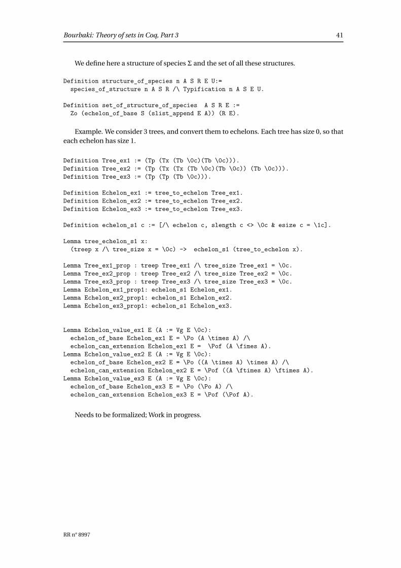


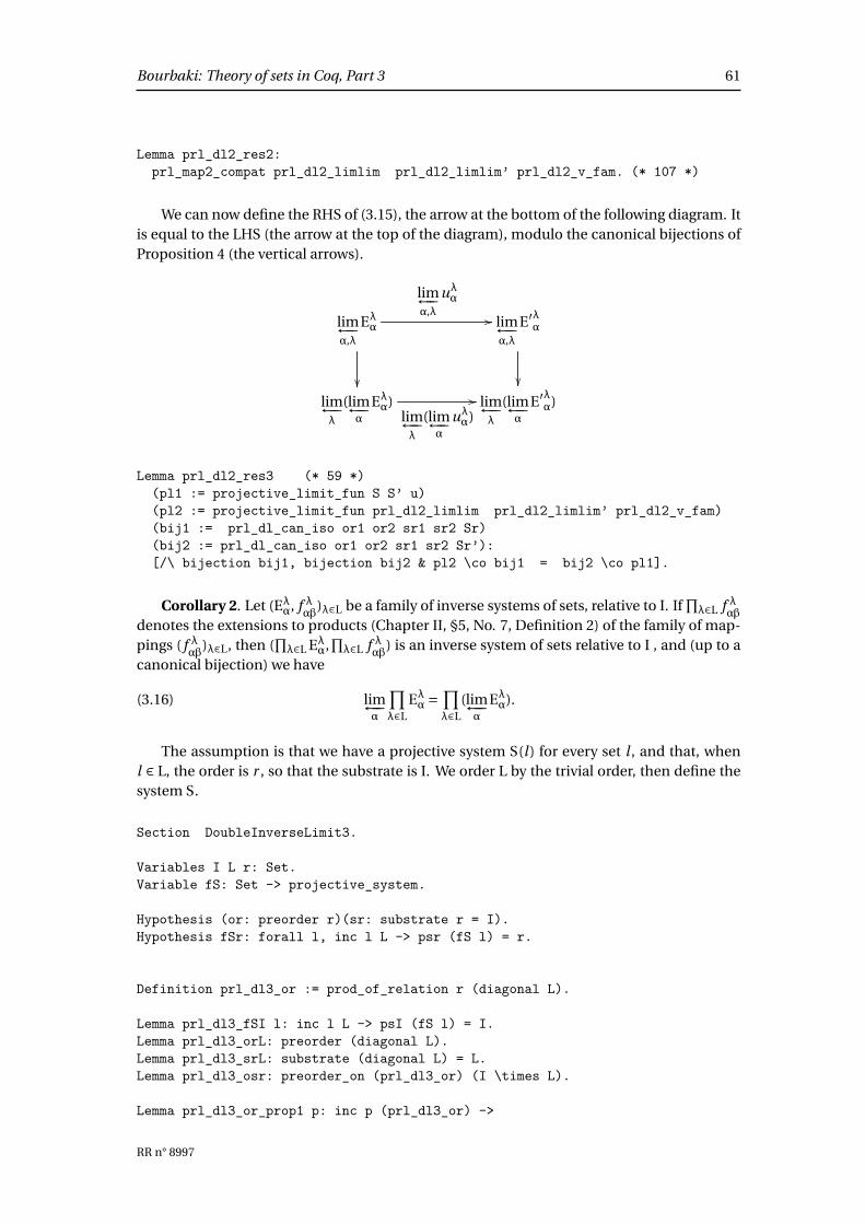


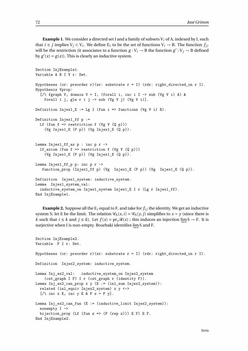
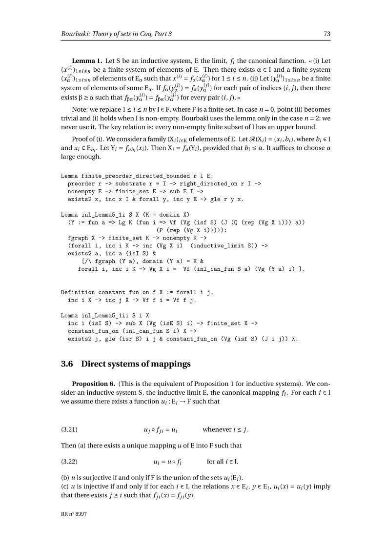


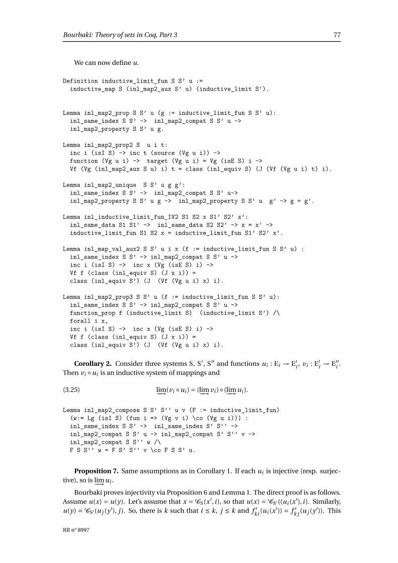
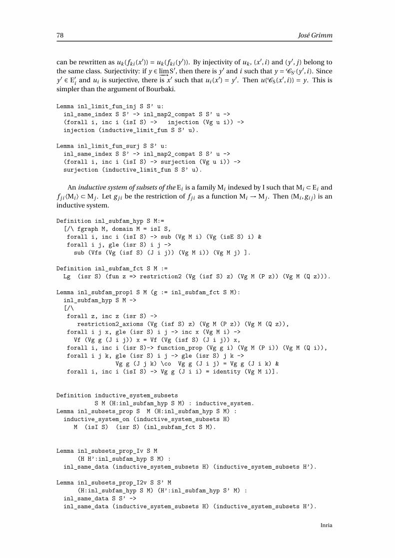


![[N.Bourbaki] Elements Of Mathematics-Algebra Part1](https://static.documents.pub/doc/80x56/577cdcc31a28ab9e78ab57b6/nbourbaki-elements-of-mathematics-algebra-part1.jpg)


