mplementation of fast-Fourier-transform-basedimulations of extra-large atmospheric phase andcintillation screens
iorgio Sedmak
Fast-Fourier-transform-based simulations of single-layer atmospheric von Karman phase screens andKolmogorov scintillation screens up to hundreds of meters in size were implemented and tested forapplications with percent range accuracy. The tests included the expected and the observed structureand pupil variance functions; for the phase, the tests also included the Fried turbulence parameter r0
he simulation of the effects of the atmospheric tur-ulence on the formation of the images from ground-ased astronomical telescopes is widely used in theesign of optical systems and in the optimization ofpplication-oriented image processing tools.1–4 Thetmospheric turbulence can be modeled as a randomrocess of known spatial and temporal characteris-ics that deteriorate the modulus and the phase of theomplex generalized pupil function.5 Several meth-ds, mainly modal and sample based, are availableor the simulation of atmospheric phase and scintil-ation screens of sizes of the order of meters.1,2,6,7 Ithould be noted that modal phase simulation meth-ds based on Zernike polynomials can be directlysed for the design of ground-based optical systems.1ther modal methods and the sample-based methodsre generally used to implement simulated observa-ions for the evaluation of optical systems and image
The author �[email protected]� is with the Dipartimento distronomia, Universita di Trieste, Via G. B. Tiepolo 11, Trieste4131, Italy.Received 23 October 2003; revised manuscript received 13 April
rocessing procedures by means of numerical modelsf the image formation process.2–4
Only a limited effort was paid to the simulation andvaluation of the quality of the extra-large screens ofnterest to the extra-large telescopes now under de-elopment for future ground-based astronomy, suchs the 30-m California Extremely Large TelescopeCELT�8 and the European Southern Observatoryverwhelmingly Large �OWL� 100-m Telescope.9 Inarticular, the simulation of extra-large scintillationcreens can help in the design of telescopes, cameras,nd software tools that are specialized for applica-ions of ultrahigh contrast range such as the detec-ion of extrasolar planets.10
Among the available methods, those based on theast Fourier transform �FFT� are less constrained byomputer memory size, numerical truncation errors,nd computing time limits that may affect otherethods. The FFT-based methods are appropriate
nly for sample-based and quasi-monochromatic,ime-correlated, single-layer simulations. More re-listic spatial and temporal characteristics can bemplemented by the sum of many single-layer simu-ations.2,11 Moreover, the FFT-based simulationsndersample the lower and higher spatial frequen-ies, and the corresponding powers need to be com-ensated to obtain a higher accuracy.3In this paper I report on the implementation and
valuation of the accuracy of compensated FFT-based
imulations of extra-large, single-layer, quasi-onochromatic phase and scintillation screens up to
undreds of meters in size for applications with sub-ercent to percent range accuracy.
. Simulation of Extra-Large Atmospheric Phasecreens
he sample-based simulations of extra-large phasecreens up to hundreds of meters in size need theupport of at least 1024 � 1024 pixels for adequateampling. The FFT-based method of McGlamery6
roved to be the most effective for such applications.he phase screen is obtained by the inverse Fourier
ransform of the product of an Hermitian complexormal noise and the square root of the phase spec-rum. For ground-based astronomical applications,he atmospheric phase spectrum can be approxi-ated by the von Karman spectrum.2,3
P�� f � � 0.00058r0�5�3� f 2 � 1�L0
2��11�6 , (1)
here P� is the spectral power, f is the spatial fre-uency, L0 is the outer scale length, and r0 is theuasi-monochromatic Fried turbulence parameter0
12:
r0 � 0.185�6�5 �cos z�3�5��0
�
Cn2�h�dh��3�5
, (2)
here � is the wavelength, z is the zenith distance,nd Cn
2�h� is the structure constant of the atmo-phere at height h from the ground. The spectrumhown by Eq. �1� assumes zero for the inner scaleength, which is typically much smaller than r0.his approximation does not affect significantly theuality of the phase simulations because of the fastoll-off of the spectrum. At infinite L0 the von Kar-an spectrum degenerates to the Kolmogorov spec-
rum.The FFT-based phase screen can be computed by
he modified Johansson and Gavel equations3:
mnFFT �
m��Nx�2
Nx�2�1
n��Ny�2
Ny�2�1
TmnHmnFmnFFT
� exp�i2 �mm�Nx � nn�Ny��,
�m � � Nx�2, Nx�2 � 1�,
�n � � Ny�2, Ny�2 � 1�,
Tmn � 1, �m��Nx�2��2 � �n��Ny�2��2 � 1,
Tmn � 0, �m��Nx�2��2 � �n��Ny�2��2 � 1,
FmnFFT � 0.1513�Gx Gy�
�1�2r0�5�6��m�Gx�
2 � �n�Gy�2
� 1�L02��11�12 , (3)
here �mnFFT is the FFT-based phase, �Nx, Ny� is the
ormat of the support in pixels, Tmn is an antialias-ng binary mask, Hmn is an Hermitian complex nor-
al �0, 1� noise, FmnFFT is the square-root von Karman
pectrum with FmnFFT � 0, for �m, n � 0�, and �Gx, Gy�
s the size of the phase screen in meters. The phase
creen is assumed to be sampled at constant step � �x � Gx�Nx � �y � Gy�Ny.If required, a more refined model of the phase spec-
rum can be obtained with a different expression ofmnFFT in Eqs. �3�, for example, to include the effects ofonzero inner scale lengths.The FFT-based simulations are accurate only for
arge values of the ratios of the screen size to theample size and of the screen size to the outer scaleength. In general, the effects of the high-frequencyndersampling are not severe because of the spectraloll-off, but subharmonic phase screens must bedded to compensate for the low-frequency under-ampling, particularly for the Kolmogorov spectrum.The effects of undersampling on the structure func-
ions of typical FFT-based simulations of extra-largehase screens of the square format �G � Gx � Gy� arehown in Fig. 1. For rectangular screens the resultsre substantially the same but for the loss of circularymmetry of the structure functions.13 The struc-ure functions were computed through the autocor-elations to obtain directly the expected valuesithout the need to average large sets of statistically
ndependent realizations. The expected structureunction D� is defined by3,12
D��r� � 2�B��0� � B��r�� , (4)
here r is the separation and B��r� is the autocorre-ation implemented by the FFT of �Fmn
FFT �2. To showhe details, the data were normalized to the theoret-cal phase structure functions3,12,14 and plotted on aemilog scale.The data show the well-known underestimate at
arge separations for large values of the ratio of theuter scale length to the screen size and the under-stimate at small separations due to the undersam-ling of the high spatial frequencies. Both effects
ig. 1. Expected structure functions Dexp normalized to the the-retical values of extra-large phase screens simulated with theFT-based method of McGlamery6 for a von Karman spectrum andhe Kolmogorov spectrum. The theoretical structure functionKolm for the Kolmogorov spectrum is shown for reference.
c2
A
Tmfsa6ammommsct
otshspcetcma
cnJi
�
wsi�
ctss
w�Fitcigpmm��
i�r�a�
aftlfpiwLt
wtwtoasposob
an be compensated for as is shown in Subsections.A and 2.B.
. Compensation at Low Frequencies
he compensation at low frequencies can be imple-ented effectively by means of a constant log-
requency spacing of the sampled phase spectrumuch as done by Lane et al.15 using a kernel of base 3nd by Johansson and Gavel3 using a kernel of base. The accuracy of the compensation improves up ton optimum by an increase in the number of subhar-onics and then saturates. The number of subhar-onics at optimum is proportional to the ratio of the
uter scale length to the screen size. For the Kol-ogorov spectrum this number is limited by the nu-erical overflow, which typically occurs at the 17th
ubharmonic for double precision floating point cal-ulations. The computing times are proportional tohe square of the kernel base.
The subharmonic phase screen must be evaluatedn the FFT support by means of a discrete Fourierransform, which is time consuming for extra-largeupports and it unnecessarily oversamples the sub-armonic range. Computing the subharmoniccreen on a subsampled FFT support and then inter-olating on the full FFT support allows for acceptableomputing times for extra-large supports. It is nec-ssary to use fast local algorithms so as to not loosehe computing time gained by subsampling. The ac-uracy is maintained if the interpolation approxi-ates the sinc weighting as done in bicubic
lgorithms, for example.The equations for the subsampled subharmonic
ompensation for the von Karman spectrum with ker-els of base modulo 3, modified and restyled fromohansson and Gavel3 and Sedmak,13 are the follow-ng:
�mn � �mnFFT � interp��rs
SUB, �m, n�,�Nx, Ny��,
�m � � Nx�2, Nx�2 � 1�,
�n � � Ny�2, Ny�2 � 1�,
rsSUB �
p�1
Np
wp m��NS�2
NS�2�1
n��NS�2
NS�2�1
HpmnFpmnSUB
� exp�i2 3�p��m � a�r�Nx � �n
� a�s�Ny��, �r � � Nx�2, Nx�2,
step�Nx�b��, �s � � Ny�2, Ny�2,
step�Ny�b��, b � 2,
FpmnSUB � 0.1513�Gx Gy�
�1�2r0�5�63�p
� ��3�p�m � a��Gx�2
� �3�p�n � a��Gy�2 � 1�L0
2��11�12 , (5)
here �mn is the compensated phase, �rsSUB is the
ubsampled subharmonic phase, interp is a bicubicnterpolator, Hpmn is a Hermitian complex normal0,1� noise, N is the number of subharmonics, a is a
p
onstant, wp is a weight factor defined below, NS ishe size of the subharmonic kernel, and Fpmn
SUB is theubharmonic square-root von Karman spectrum. Theubsampling step b is conveniently set equal to eight.The original method of Lane et al.15 is implementedith NS � 3, Fpmn
SUB � 0 for �m, n � 0�, a � 0, and wp1 and does not use any patch normalization of
mnFFT. However, to obtain the maximum accuracy it
s necessary to patch normalize FmnFFT for the leakage
hrough the secondary lobes of the spectral windoworresponding to the subharmonic bin. The normal-zation weights can be computed by means of inte-rating numerically the spectral window over theatch overlap of the FFT and the subharmonic do-ains. The patch normalization is then imple-ented by the weighting of Fmn
FFT by 0.935 for �m, n�1, 0� and �m, n � 0, �1� and by 0.998 for �m, n�1, �1�.The original method of Johansson and Gavel3 is
mplemented with NS � 6, FpmnSUB � 0 for �m, n �
1, 0� and �m, n � 0, �1�, a � 0.5, and wp � 1 andequires us that Fmn
FFT be patch normalized by one halfweight 0.707� for �m, n � �1,0� and �m, n � 0, �1�nd three fourths �weight 0.866� for �m, n � �1,1�.The method of Johansson and Gavel allows one to
pproximate quite well the theoretical structureunction up to an infinite outer scale length. Herehe method of Lane et al.15 fails because of insufficientow-frequency sampling. However, the relativelyaster execution time and the smaller numericalroblems make the method of Lane et al. competitivef the residual undersampling is compensated. Theeights required to compensate the subharmonics ofane et al. can be computed by the following equa-
ions:
wp � �Pptot��Pp
tot � Pp0��1�2 ,
Pp0 � �
�0.5��3pGx�
�0.5��3pGx�
dfx��0.5��3pGy�
�0.5��3pGy�
dfy P� � WpLO � Wp
HI,
Pptot � �
�1.5��3pGx�
�1.5��3pGx�
dfx ��1.5��3pGy�
�1.5�3pGy�
dfy P� � WpLO � Wp
HI,
WpLO � sinc2� fx3
pGx�sinc2� fy3pGy�,
WpHI � sinc2� fx3
p�1Gx�sinc2� fy3p�1Gy� , (6)
here wp is the weight for the p subharmonic, P� ishe phase spectrum, Wp
LO and WpHI are the spectral
indows corresponding to the screen and the pixel ofhe subharmonic kernel, and R is the convolutionperator. The weights’ result is independent of r0nd can be further optimized by the compensatedtructure function if required. The weights com-uted for the first ten subharmonics at various valuesf the ratio of the outer scale length L0 to the screenize G are shown in Table 1. The weights for valuesf the ratios other than those contained in Table 1 cane easily computed mapping the data of Table 1.
he compensation at high frequencies is less criticalecause it affects only the smallest spatial scale sety the sample size of the screen. The compensationan be implemented by the weighting of the compo-ents of Fmn
FFT so as to add at the folding frequency theower lost at higher frequencies. However, it is con-enient to distribute this extra power on a smallandwidth, typically 1% of the full range to minimizehe truncation ripple with a suitable apodizationunction like a Gaussian half-bell. The weight cane computed by the following equation:
whi � �1 � �fn
�
fP�� f �df��fn�bw
fnfP�� f �df�1�2
, (7)
here whi is the weight, fn � 0.5�� is the foldingrequency, and bw is the apodization bandwidth.he weight is independent of r0, L0, and of the screenize; it depends only on the support size and thepodization bandwidth. For N � 1024 and bw � 5,he weight approximates 7.8. The weighting is con-eniently implemented when the term Tmn in Eqs.3� is replaced with �whi Tmn� over the apodizationandwidth. The weight can be further optimized byhe compensated phase structure function if re-uired.One sample phase screen simulated with the FFT-
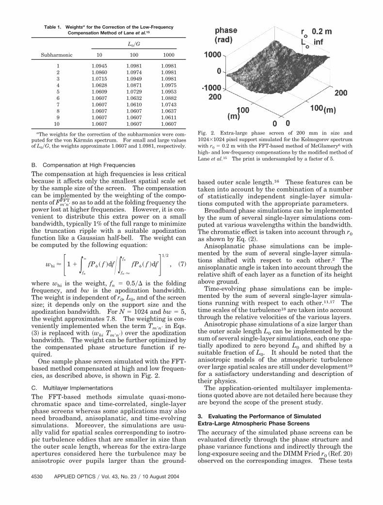
ased method compensated at high and low frequen-ies, as described above, is shown in Fig. 2.
. Multilayer Implementations
he FFT-based methods simulate quasi-mono-hromatic space and time-correlated, single-layerhase screens whereas some applications may alsoeed broadband, anisoplanatic, and time-evolvingimulations. Moreover, the simulations are usu-lly valid for spatial scales corresponding to isotro-ic turbulence eddies that are smaller in size thanhe outer scale length, whereas for the extra-largepertures considered here the turbulence may benisotropic over pupils larger than the ground-
Table 1. Weightsa for the Correction of the Low-FrequencyCompensation Method of Lane et al.15
aThe weights for the correction of the subharmonics were com-uted for the von Karman spectrum. For small and large valuesf L0�G, the weights approximate 1.0607 and 1.0981, respectively.
ased outer scale length.16 These features can beaken into account by the combination of a numberf statistically independent single-layer simula-ions computed with the appropriate parameters.
Broadband phase simulations can be implementedy the sum of several single-layer simulations com-uted at various wavelengths within the bandwidth.he chromatic effect is taken into account through r0s shown by Eq. �2�.Anisoplanatic phase simulations can be imple-ented by the sum of several single-layer simula-
ions shifted with respect to each other.2 Thenisoplanatic angle is taken into account through theelative shift of each layer as a function of its heightbove ground.Time-evolving phase simulations can be imple-ented by the sum of several single-layer simula-
ions running with respect to each other.11,17 Theime scales of the turbulence18 are taken into accounthrough the relative velocities of the various layers.
Anisotropic phase simulations of a size larger thanhe outer scale length L0 can be implemented by theum of several single-layer simulations, each one spa-ially apodized to zero beyond L0 and shifted by auitable fraction of L0. It should be noted that thenisotropic models of the atmospheric turbulencever large spatial scales are still under development19
or a satisfactory understanding and description ofheir physics.
The application-oriented multilayer implementa-ions quoted above are not detailed here because theyre beyond the scope of the present study.
. Evaluating the Performance of Simulatedxtra-Large Atmospheric Phase Screens
he accuracy of the simulated phase screens can bevaluated directly through the phase structure andhase variance functions and indirectly through theong-exposure seeing and the DIMM Fried r0 �Ref. 20�bserved on the corresponding images. These tests
ig. 2. Extra-large phase screen of 200 mm in size and024�1024 pixel support simulated for the Kolmogorov spectrumith r0 � 0.2 m with the FFT-based method of McGlamery6 withigh- and low-frequency compensations by the modified method ofane et al.15 The print is undersampled by a factor of 5.
ccdewCoabcttrv�a
bfcatfKJtmwmtwsm
A
F1artetdndltpstesc
waTmfs
rt�BebTmGi1t
r
opGcawt
FfltfGt
omplement and complete each other for astronomi-al applications. The tests reported here were un-ertaken for the Kolmogorov spectrum because itxploits the limits of the simulations. Several testsere also undertaken for the von Karman spectrum.losely similar results were obtained, and some testsf simulated von Karman phase structure functionsre reported here for completeness. Where applica-le, a large number of simulations was used to de-rease the relative statistical deviation of the resultshat, for a normal distribution, is approximated byhe reciprocal of the square root of the number ofealizations. All simulations were performed with aalue r0 � 0.2 m, which corresponds to a seeing of0.55 arc sec of full width at half-maximum �FWHM�t the wavelength of 550 nm �V band�.The simulations were performed with the FFT-
ased method of McGlamery6 with high- and low-requency compensations. The high-frequencyompensation was performed as described above withn optimized weight of 8.2 and a Gaussian apodiza-ion half-bell bandwidth of 5 bins. The low-requency compensation was performed in theolmogorov case with either the original method ofohansson and Gavel3 with 15 subharmonics or withhe modified method of Lane et al.15 with 10 subhar-onics and patch normalized with corner and sideeights of 0.998 and 0.935, respectively, and opti-ized with a subharmonic weighting of 1.106. In
he von Karman case, three and five subharmonicsere used for the two methods, respectively, with a
ubharmonic weighting of 1.061 for the modifiedethod of Lane et al.
. Phase Structure and Phase Variance Functions
or the tests, a screen size of 200 m and a support of024 � 1024 pixels were used with an r0 of 0.2 m andn infinite L0. The results of the tests are summa-ized in Table 2. The expected and observed struc-ure functions are shown in Figs. 3 and 4. Thexpected structure functions are noiseless by defini-ion but are not computed on the actual simulatedata. The observed structure functions show a sig-ificant dispersion but are computed on the actualata and can detect any simulation-dependent prob-em possibly masked in the expected structure func-ions. For this reason the tests reported here wereerformed with either the expected or the observedtructure functions. The expected structure func-ions were computed through the autocorrelations forither the FFT-based or the subharmonic phasecreens. The observed structure functions wereomputed by the equation.3,12
D��r�� � ����r� � r�� � ��r���2� , (8)
ith the results averaged over 1100 realizations forn expected normal deviation of the mean of 3%.he assumption of normal distribution is approxi-ately valid because the deviations of the structure
unctions are dominated by the contributions at lowerpatial frequencies.
The expected structure functions match the theo-etical values closely with a rms error of �0.38% forhe original method of Johansson and Gavel3 and of0.15% for the modified method of Lane et al.15
oth methods show evidence of a residual loss of thexpected values less than 1% at lower frequenciesecause of the finite number of subharmonics used.he expected structure function reported for the Kol-ogorov spectrum in the paper of Johansson andavel shows a small extra underestimate of approx-
mately �1% at 1 m, which increases up to �5% at00 m, probably because of a wrong patch normaliza-ion that was corrected in the current paper.
The observed structure functions match the theo-etical values with a rms error of �0.86% for the
Table 2. Errors of the Phase Structure and Phase Variance Functionsof the Simulationsa
Parameter Error
Simulator
A B
Dexp�Dtheor rms 0.0038 0.0015L0 � � Maximum 0.0092 0.0035Dobs�Dtheor rms 0.0086 0.0108L0 � � Maximum 0.0257 0.0205��obs
2 ��� theor2 rms 0.0087 0.0077
L0 � � Maximum 0.0233 0.0213Dexp�Dtheor rms 0.0009 0.0005L0 � 25 m Maximum 0.0093 0.0092
aThe rms and maximum errors of the normalized expected andbserved phase structure and phase variance functions were com-uted on simulations obtained with the FFT-based method of Mc-lamery6 compensated at high frequency and with low-frequency
ompensation by �A� the original method of Johansson and Gavel3nd �B� the modified method of Lane et al.15 The phase screensere simulated with r0 � 0.02 m, L0 � infinity �Kolmogorov spec-
rum�, and L0 � 25 m �von Karman spectrum�.
ig. 3. �a� Expected Dexp and �b� observed Dobs phase structureunctions �thick curves� normalized to theoretical values of extra-arge phase screens simulated for the Kolmogorov spectrum withhe FFT-based method of McGlamery6 with high- and low-requency compensations by the original method of Johansson andavel.3 The expected and observed standard deviations above
ethod of Johansson and Gavel and of �1.08% forhe modified method of Lane et al.
For completeness the expected structure functionsere also computed for the von Karman spectrumssuming an outer scale length L0 � 25 m. Theesults are reported in Fig. 5 and Table 2 and show ams error of �0.09% for the method of Johansson andavel and of �0.05% for the modified method of Lane
t al.The phase variance was computed on circular pu-
ils of aperture up to the phase screen size, and theesults were averaged over 1100 realizations. Theinimum aperture was set to 1% of the phase screen
ig. 4. �a� Expected Dexp and �b� observed Dobs phase structureunctions �thick curves� normalized to theoretical values of extra-arge phase screens simulated for the Kolmogorov spectrum withhe FFT-based method of McGlamery6 with high- and low-requency compensations by the modified method of Lane et al.15
he expected and observed standard deviations above the meanre also shown �thin curves�.
ig. 5. Expected phase structure functions Dexp normalized toheoretical values of extra-large phase screens simulated for theon Karman spectrum with the FFT-based method of McGlamery6
ith high- and low-frequency compensations by �a� the originalethod of Johansson and Gavel3 and �b� the modified method ofane et al.15
ize to properly sample the pupil. The results nor-alized to the theoretical values given by Fried21 are
hown in Figs. 6 and 7. The data confirm the accu-acy of the simulations with a mean error of �0.87%or the method of Johansson and Gavel and of0.77% for the modified method of Lane et al.
. Long-Exposure Seeing and Differential Image Motiononitor r0he long-exposure seeing probes the medium to
arge-scale properties of the phase screens. Theimulations were performed with an r0 of 0.2 m andn infinite L0. I computed the long-exposure seeingy averaging over 1100 realizations the speckles gen-rated with a circular pupil of an aperture of one half
ig. 6. Observed phase variance function normalized to theoret-cal values of extra-large phase screens simulated for the Kolmog-rov spectrum with the FFT-based method of McGlamery6 withigh- and low-frequency compensations by the original method ofohansson and Gavel.3 The expected �thin curves� and observedbars� standard deviations above the mean are shown for reference.
ig. 7. Observed phase variance function normalized to theoret-cal values of extra-large phase screens simulated for the Kolmog-rov spectrum with the FFT-based method of McGlamery6 withigh- and low-frequency compensations by the modified method ofane et al.15 The expected �thin lines� and observed �bars� stan-ard deviations above the means are shown for reference.
owsSasoasb
Tsuimp
ostrseoptmraTcF
papcE
t0D2msttGuecDan
O
�cmmto
FehtGis
f the screen size. For these tests the screen sizeas set equal to 50 m to sample the screens at four
amples per r0 on a support of �1024 � 1024� pixels.ome extra tests were done on screens of a size of 100nd 200 m to explore the effects of sampling thecreens at two and one samples per r0. The FWHMf the seeing was estimated by the Gaussian fit of theverage of the X and Y sections at the center of theeeing image, and the corresponding r0 was computedy the equation20
r0�m� � 0.98��m��FWHMseeing�rad�
� 0.98G�m��FWHMseeing�pixel� . (9)
he results of the tests are reported in Table 3. Oneample of the sections of a long-exposure seeing sim-lated with a fully compensated FFT-based method
s shown in Fig. 8. The core of the data closelyatch a Gaussian of FWHM equal to the value com-
uted by Eq. �9� for the theoretical r0.The uncompensated FFT-based phase simulations
verestimate the theoretical r0 computed from theeeing image by �11%. This effect is mainly due tohe lack of low-frequency power because the sameesult was obtained with the high-frequency compen-ation only. The undersampling increases the over-stimate up to �17% at two samples and �79% atne sample per r0. The results with adequate sam-ling with either high or low-frequency compensa-ions are much better, resulting in a deviation of theean no larger than 0.1% for both methods. The
esults are consistent with the signal-to-noise ratiost half-height of the sections of the seeing images.hese results confirm the need of the low-frequencyompensation for astronomical applications of theFT-simulated phase screens.The differential image motion monitor �DIMM�r0
robes the small-scale properties of the phase screensnd rejects by design the low-spatial-frequency com-onents. The DIMM device was simulated with twoircular pupils a 0.05 m in size separated by 0.25 m.very phase screen was sampled on 28 positions and
aThe long-exposure seeing r0 and DIMM r0 were averaged on tim0.2 m and L0 � infinity �Kolmogorv spectrum� with �A� the unc
ompensated at high frequency, �C� the same method compensateethod of Johansson and Gavel,3 and �D� the same method comodified method of Lane et al.15 The FWHMs of the seeing ima
o-noise ratios �SNRs� of the seeing images were evaluated at halff r0 were computed from the best-fitted log-normal distributions.
ime shifted according to Taylor hypothesis22 by.01 s with a screen shift speed of 10 m�s. TheIMM image was interpolated to a support of 256 �56 pixels from a subimage of constant size of 3.125
extracted from the center of the phase screens toample properly the DIMM pupils independently ofhe phase screen size and sampling. The centers ofhe images from the two pupils were estimated by aaussian fit to subpixel accuracy. The equationssed to compute r0 from the variances of the differ-ntial transverse and longitudinal distances of theenters were those of Sarazin and Roddier.20 TheIMM r0 was then averaged over 300 realizations forn equivalent observing time of 84 s and an expectedormal deviation of the mean of 5.8%.The results of the tests are reported in Table 3.ne sample histogram of DIMM r0 data simulated
rrelated speckles computed from phase screens simulated with r0ensated FFT-based method of McGlamery,6 �B� the same methodhigh frequency with low-frequency compensation by the originalated at high frequency with low-frequency compensation by theas computed from the best-fitted normal functions. The signal-ht of the images. The mean values and the standard deviations
ig. 8. Normalized intensity section at the center of a long-xposure seeing image obtained by a pupil with a diameter of onealf of the screen size from extra-large phase screens simulated forhe Kolmogorov spectrum with the FFT-based method of Mc-lamery6 with high- and low-frequency compensations by the mod-
fied method of Lane et al.15 The normal of FWHM �r0 � 0.2 m� ishown for reference.
ith a fully compensated FFT-based method ishown in Fig. 9. The data approximate a log-normalistribution in good agreement with the observationsf Wilson et al.23 The uncompensated FFT-basedhase simulations overestimate the DIMM r0 by13.3%. The data computed with only the high-
requency compensation show a clear improvementith the deviation of the mean reduced to �3.7%.ndersampling the screens increases dramatically
he deviations, overestimating the DIMM r0 by �52%t two samples and �150% at one sample per r0. Asxpected the low-frequency compensation does nothange the results significantly. The deviations ofhe mean DIMM r0 result are �3.5% for the methodf Johansson and Gavel and �4% for the modifiedethod of Lane et al. Further tests done on screens
f a 12.5 m in size at 16 samples per r0 produced meanIMM r0 values also within one standard deviation of
he theoretical values. These results confirm theeed of adequate sampling and of high-frequencyompensation of the FFT-simulated phase screens.
. Performance
he phase structure, phase variance, long-exposureeeing, and DIMM r0 data reported above show thathe FFT-based simulations of extra-large phasecreens up to hundreds of meters in size can be im-lemented successfully from subpercent to percentccuracy. This high accuracy is obtained when thehase screen is sampled with at least four sampleser r0 and by appropriate high- and low-frequencyompensations and patch normalization. The extra-arge screens considered here need typical supportsrom 1024 � 1024 up to 4096 � 4096 pixels in theisual spectral range. The modified subharmonicompensation method of Lane et al. outperforms theriginal method of Johansson and Gavel in terms of
ig. 9. Histogram of r0 data obtained by a simulated DIMM de-ice from extra-large phase screens simulated for the Kolmogorovpectrum with the FFT-based method of McGlamery6 with high-nd low frequency compensations by the modified method of Lanet al.15 The log normal with the mean and standard deviationqual to the observed values is shown for reference.
he structure functions, although the two methodsre comparable in terms of the phase variance, theong-exposure seeing FWHM, and the DIMM Fried0.
The computing times are dominated by the FFTimes for the FFT-based phase screen and by thewo-dimensional interpolation time for the sub-ampled subharmonic screen. The execution time ofne simulation of 1024 � 1024 pixel support imple-ented in MATLAB was approximately 14 s on a Pen-
ium 4 running at 2500 MHz with 512-Mbytes RAMemory. Typically 36% of the time was spent for
he preparation of the working arrays; 21% for theFT, and 43% for the bicubic interpolation.For comparison, the computing time of an equiva-
ent phase screen simulated for a pupil with a 10-mperture and 512 � 512 pixel support by means of anDL implementation of the Zernike polynomialsethod of Roddier1 in the Kolmogorov case with 50
adial orders, corresponding to approximately oneample per r0, was approximately 72 s on the samelatform. For a MATLAB implementation of theourier-series method of Welsh2 it was approxi-ately 4 s for L0 � 25 m with 375 coefficients and
pproximately one sample per r0, increasing to ap-roximately 450 s for L0 � 250 m with 3750 coeffi-ients and approximately 12 r0 per sample i.e., withevere undersampling. The computing times forhese modal methods are dominated by the number ofoefficients. For the extra-large apertures consid-red here, this may force one to undersample thehase screen to avoid numerical, memory, and com-uting time limits.Parallel platforms based on clusters of nodes �Be-
wulf clusters24� were also used for the FFT methodnd allowed a relative speed gain close to the numberf nodes for the computation of a series of sequentialimulations. The parallel platforms can then beseful for the simulation of multilayer atmospherichase screens or time series of atmospheric speckles.
. Simulation of Extra-Large Atmospheric Scintillationcreens
he numerical simulation of extra-large scintillationcreens to be possibly used together with phasecreens up to hundreds of meters in size can be alsomplemented by means of the FFT-based method de-cribed in Section 2 with Eqs. �10� for the scintillationpectrum12,25 valid for Kolmogorov turbulence andero inner scale length near zenith with negligibleaturation:
S� f � � 1.54��2A� f � f �11�3 k�1
NL
Cn2�hk��hk
� sin2� �hf 2�,
A� f � � �2J1� Df ��� Df ��2 , (10)
here S�f � is the spectrum, f is the spatial frequency,is the wavelength, A�f � is the spatial filter corre-
ponding to the unobstructed circular pupil of aper-
tfsCcga
�Eimoflwpi
iopwa
atmwm
lltst
aCi
wt�
zlcE
qd21anbir
tca
s
F
wtaniit
toci
svSitR
ssorortt
os
ure D in meters of the telescope, J1 is the Besselunction of first order, NL is the number of atmo-pheric layers of thickness �hk considered, andn
2�hk� are the corresponding values of the structureonstant of the atmosphere at the heights hk from theround. The spectrum given by Eqs. �10� vanishest zero frequency.It should be noted that the von Karman correction
f2 � 1�L02��11�6 to the Kolmogorov term f�11�3 in
qs. �10� is not used because the scintillation is dom-nated by higher atmospheric layers that approxi-
ate the Kolmogorov turbulence. For large valuesf L0 the effect is to increase the slope toward zerorequency and then decrease the total power, with aoss of approximately 11% for L0 � 250 m and a pupilith a 50-m aperture. This loss can be easily com-ensated for by means of the scaling constant S0 usedn Eqs. �12� to normalize the scintillation index.
It should also be noted that the inner scale lengths assumed to be zero because it affects significantlynly the higher spatial frequencies where the spectralower is substantially rejected by the pupil filter,hich shows a strong damping for the extra-largepertures considered here.Finally, the saturation is assumed negligible for
pplications to ground-based astronomical observa-ions near the zenith during the night following theeasurements of Vernin reported by Roddier,12
hich show a median scintillation index of approxi-ately 0.2 with only occasional values above 0.5.The von Karman correction, the finite inner scale
ength term, and possibly the saturated regime atarge zenith distances should be included in the spec-rum for extremely accurate simulations of the atmo-pheric scintillation, which are beyond the scope ofhis study.
Because the scintillation is dominated by highertmospheric layers, a suitable approximation ofn
2�h� to be used in the spectrum given by Eqs. �10�s the model of Hufnagel26:
Cn2�h� � c0
2r0�5�3�2 ����2��h�h0�
10 exp� � h�h1�
� exp� � h�h2�� , (11)
here r0 is the quasi-monochromatic Fried parame-er given by Eq. �2�, c0
2 � 1.027 � 10�3 h0 � 4632, h11000, and h2 � 1500.The chromatic effects and the dependence from the
enith distance within the limits of the weak turbu-ence regime of interest to ground-based astronomyan be taken into account through r0 and Cn
2�h� inqs. �2� and �11�.The scintillation spectrum given above matches
uite well the observational data reported by Rod-ier12 for NL � 2 when we use the values h1 �250 m, �h1 � 3600 m, and h2 � 10,000 m, �h2 �0,000 m, for the two layers, determined by Ochs etl.27 It should be noted that the Hufnagel model isot realistic because Cn
2�h� is concentrated in a num-er of thin layers28 but it is sufficient here to approx-mate the values of Cn
2�h� integrated over theelatively broad layers used in Eqs. �10� according to
he scheme of Ochs et al.27 If required, a more ac-urate model can be obtained by use of more layersnd the observed values of Cn
2�h�.The equations for the FFT-based simulation of a
cintillation screen can be written as follows:
SmnFFT �
m��Nx�2
Nx�2�1
n��Ny�2
Ny�2�1
Tmn Hmn FmnFFT
� exp�i2 �mm�Nx � nn�Ny��,
�m � � Nx�2, Nx�2 � 1�,
�n � � Ny�2, Ny�2 � 1�,
mnFFT � �Gx Gy�
�1�2[So1.54 ��2��m�Gx�2
� �n�Gy�2��11�6(2J1� D��m�Gx�
2
� �n�Gy�2�1�2��� D��m�Gx�2
� �n�Gy�2�1�2�)2
� k�1
NL
Cn2�hk��hk sin2� �hk��m�Gx�
2
� �n�Gy�2��]1�2 , (12)
here SmnFFT is the FFT-based scintillation, �Nx, Ny� is
he format of the support in pixels, Tmn is the anti-liasing binary mask, Hmn is a Hermitian complexormal �0,1� noise, Fmn
FFT with FmnFFT � 0 for �m, n � 0�
s the FFT-based square-root scintillation spectrum, S0s a normalization constant, and �Gx, Gy� is the size ofhe scintillation screen in meters.
If required, a more refined model of the scintilla-ion spectrum can be obtained, when the expressionf Fmn
FFT is replaced in Eqs. �12�, for example, to in-lude the effects of finite outer scale and nonzeronner scale lengths.
The constant S0 scales the spectrum for the wantedcintillation index �normalized intensity variance� atanishing aperture. For r0 � 0.147 m, � � 550 nm,0 � 1, and the simulated scintillation index approx-
mates 0.2, which corresponds to the peak of the his-ogram of the observations of Vernin reported byoddier.12
The expected structure functions of FFT-basedimulations of extra-large scintillation screens ofquare format �G � Gx � Gy�, normalized to the the-retical values, are shown in Fig. 10. The autocor-elation required by Eq. �4� was computed by the FFTf the term �Fmn
FFT �2 in Eqs. �12�. The autocorrelationequired to evaluate the theoretical structure func-ion was computed by the numerical integration ofhe equation28,29
Bs�r� � 2 �0
�
S� f �J0�2 fr� fdf , (13)
btained by the Hankel transform of the scintillationpectrum where r is the separation, B �r� is the au-
FiFtstructure function Dtheor is shown for reference.
Flmsspectral details.
4
ocorrelation, S�f � is the scintillation spectrum, and0 is the Bessel function of order zero.The structure functions of Fig. 10 show that the
cintillation spectrum is well sampled for screen sizesarger than eight times the pupil size, whereas theres a strong underestimate at large separations atcreen sizes equal to the pupil size. Moreover, theres an overestimate at smaller separations that de-reases as the ratio of the screen size to the pupilperture increases; for extra-large pupils, the scintil-ation spectrum, which is highly oscillatory becausef the Bessel term, peaks at the harmonics of theaximum in the frequency range �0, 1�D� whereas
he FFT-based spectrum is sampled only at multiplesf 1�G. The theoretical and sampled scintillationpectra are shown in Fig. 11 for two values of theatio of the screen size to the pupil aperture. Theata of Fig. 11 show how the undersampling losesow-frequency power and generates the bias found onhe structure functions when the spectral details areasked.Note that it is possible to work on undersampled
creens as large as the pupil and add subharmonics tohe FFT-based scintillation screen to compensate theow-frequency undersampling, but it is impossible tovoid the spectral bias. Several attempts were un-ertaken and proved that the rms accuracy of simu-ations with subharmonic compensation is generallyot better than 10% in terms of the expected struc-ure functions. Following these results, the over-ized original FFT-based method of McGlamery wassed in this study as the standard for the accurateimulation of extra-large scintillation screens.The results reported above enforce the need to usevalue of �at least� eight for the ratio of the screen
ize to the pupil aperture. For a Fried r0 � 0.2 mnd a pupil aperture of 50 m, sampling the screen atour samples per r0 as needed for the simulation ofhe phase implies for the simulation of the scintilla-
ion a screen size of 400 m and a support of 8192 �192 pixels. This format is quite large but manage-ble with commonly available computers.The data in Fig. 10 also show the underestimation
or lower separations due to the inadequate high-requency sampling. This effect can be compensatedy use of the same method reported in Section 2 forhe phase. The weight computed by approximation7� for the spectrum given by Eqs. �10� and �11� ap-roximates 10 and should be optimized with respecto the compensated structure function.
One sample scintillation screen simulated with theFT-based method compensated at high frequencies
s shown in Fig. 12.
. Performance of Simulated Extra-Large Atmosphericcintillation Screens
he accuracy of the simulated scintillation screensan be evaluated directly through the structure func-ions and the normalized intensity variance functionss was done for the phase. The simulations for theests were computed on screens with a square formatf a 400 m in size with supports of 1024�1024 pixelsor unobstructed circular pupils with an aperture of0 m. The method used was the original FFT-basedethod of McGlamery compensated at high fre-
uency with an optimized weight of 4.3. All simu-ations were performed with a value r0 � 0.2 m at aavelength of 550 nm �V band�, which corresponds toseeing of � 0.55 arc sec FWHM.The expected and observed structure functions nor-alized to the theoretical values are shown in Fig.
3. All observed data are the average of 1000 real-zations for an expected normal deviation of 3.1%.ere the normal assumption is only an upper limit to
he deviation of the mean structure functions due tohe shape of the scintillation spectrum toward zerorequency. The theoretical values were computedith Eqs. �4� and �10�–�13�. The observed structure
ig. 10. Expected structure functions Dexp normalized to theoret-cal values of extra-large scintillation screens simulated with theFT-based method of McGlamery6 at various values of the ratio ofhe screen size to the pupil aperture. The theoretical scintillation
ig. 11. Theoretical and sampled scintillation spectrum in theow-spatial-frequency range. The sampled spectrum approxi-
ates the theoretical spectrum for a value of 8 of the ratio of thecreen size to the pupil aperture, whereas a value of 2 masks the
fmafp
sm
w�ta
0aavsvast1
1aM7w
6
TKsntmcapsfrtut
nstli
Ftofi
Fsomes
Fs0ao
unctions were computed with Eq. �8�. The resultsatch the theoretical values with a 0.35% rms error
nd a 2.05% peak deviation for the expected structureunctions and with a 0.52% rms error and a 2.32%eak deviation for the observed structure functions.The observed normalized intensity variances are
hown in Fig. 14. The theoretical values of the nor-alized intensity variances �I
2 were computed by
�I2 � 2 �
0
�
fS� f �df , (14)
here S�f � is the scintillation spectrum given by Eqs.10� and �11�. The scintillation index is defined ashe limit of �I
2 at zero pupil aperture. For r0 � 0.2 mnd � � 550 nm, the scintillation index approximates
ig. 12. Extra-large scintillation screen simulated for a scintilla-ion index of 0.12 �r0 � 0.2 m at � � 550 nm� and a pupil aperturef 50 m with the FFT-based method of McGlamery with high-requency compensation. The image is the central region of 50 mn size of a screen of 400 m in size and 1024 � 1024 pixel support.
ig. 13. �a� Expected Dexp and �b� observed Dobs scintillationtructure functions �thick curves� normalized to theoretical valuesf extra-large scintillation screens simulated with the FFT-basedethod of McGlamery with high-frequency compensation. The
xpected and observed standard deviations above the mean arehown for reference �thin curves�.
.12. The theoretical normalized intensity vari-nces in the apertures ranging from 0.01 to 100 m arelso shown in Fig. 14. The data approximate thealues observed by Dravins et al.30 for a scaling con-tant S0 � 0.5. The observed normalized intensityariances were approximated directly by the vari-nces of the simulated scintillation screens. The re-ults for the normalized intensity variances matchhe theoretical values with 0.54% rms error and.45% peak deviation.The execution time of one simulation of a
024�1024 pixel support implemented in MATLAB waspproximately 17 s on a Pentium 4 running at 2500Hz with 512-Mbytes RAM memory. Typically
0% of the time was spent for the preparation of theorking arrays and 30% for the FFT.
. Conclusion
he simulations of extra-large Kolmogorov and vonarman phase screens and Kolmogorov scintillation
creens by means of the FFT-based method with patchormalization and high and low-frequency compensa-ions can be implemented effectively up to hundreds ofeters in size with an accuracy of subpercent to per-
ent range by use of large but manageable supportsnd affordable computing times. It is fundamental toroperly sample the phase screens with at least fouramples per Fried r0 and to also use the same samplingor the associated scintillation screens to adequatelyeproduce the effects of the small-scale properties ofhe atmospheric turbulence. It is also fundamental tose screen sizes of at least eight times the pupil aper-ure to adequately sample the scintillation spectrum.
The high-frequency compensation is important butot critical and can be easily implemented as de-cribed in this paper. The low-frequency compensa-ion is fundamental for the simulation of the phase atarge values of the outer scale length and particularlyn the Kolmogorov case. The method of Lane et al.15
ig. 14. Observed normalized intensity variances computed onimulated scintillation screens with pupil apertures D � Dsim from.5 to 50 m superimposed to the theoretical function evaluated forscintillation index of 0.12 �r0 � 0.2 m at � � 550 nm�. The curve
f the theoretical slope D�7�3 is shown for reference.
roved to be particularly suitable for this applicationhen modified as described in this paper.The structure functions can be used as general-
urpose quality probes on medium to large spatialcales, but it is important to also test the accuracy ofhe simulations by means of application-orientedrobes, particularly on the smaller spatial scales.he long-exposure seeing FWHMs and the DIMM r0re suitable to test the phase screens. The intensityariance over the pupil is suitable to test either thehase screens or the scintillation screens.The computing times are dominated by the FFTs
nd for the phase only by the bicubic interpolationsed for the subsampled low-frequency compensation.se of parallel platforms allowed a substantial speed
ain in the simulation of multilayer phase screens andf a series of phase and scintillation screens.
This research was performed under the cofinancedCOFIN� program, contract 2001025444_001 �2001�,f the Italian Ministry of University and Research.
eferences1. N. Roddier, “Atmospheric wavefront simulation using Zernike
polynomials,” Opt. Eng. 29, 1174–1180 �1990�.2. B. M. Welsh, “A Fourier-series-based atmospheric phase
screen generator for simulating nonisoplanatic geometries andtemporal evolution,” in Propagation and Imaging through theAtmosphere, L. R. Bissonnette and J. C. Dainty, eds., Proc.SPIE 3125, 327–338 �1997�.
3. E. M. Johansson and D. T. Gavel, “Simulation of stellar speckleimaging,” in Amplitude and Intensity Spatial Interferometry II,J. B. Breckinridge, ed., Proc. SPIE 2200, 372–383 �1994�.
4. V. V. Voitsekhovich, L. J. Sanchez, and V. G. Orlov, “Effect ofscintillation on adaptive optics systems,” Rev. Mex. Astron.Astrophys. 38, 193–198 �2002�.
5. D. L. Fried, “Optical resolution through a randomly inhomo-geneous medium for very long and very short exposures,” J.Opt. Soc. Am. 56, 1372–1380 �1966�.
6. B. L. McGlamery, “Computer simulation studies of compensa-tion of turbulence degraded images,” in Image Processing, J. C.Urbach, ed., Proc. SPIE 74, 225–233 �1976�.
7. D. Kouznetsov, V. V. Voitsckhovich, and R. Ortega-Martinez,“Simulation of turbulence-induced phase and log-amplitudedistortions,” Appl. Opt. 36, 464–469 �1997�.
8. J. E. Nelson, “Design concepts for the California ExtremelyLarge Telescope �CELT�,” in Telescope Structures, Enclosures,Controls, Assembly�Integration�Validation, and Commission-ing, T. Sebring and T. Andersen, eds., Proc. SPIE 4004, 405–419 �2000�.
9. P. Dierickx and R. Gilmozzi, “OWL concept overview,” in Pro-ceedings of Backaskog Workshop on Extremely Large Tele-scopes. T. Andersen, A. Ardeberg, and R. Gilmozzi, eds.�European Southern Observatory, Garching, Germany, 2000�,Vol. 57, pp. 43–49.
0. R. Neuhauser, W. Brandner, A. Eckart, E. W. Guenther, J.Alves, Th. Ott, N. Huelamo, and M. Fernandez, “On the pos-sibility of ground-based direct imaging detection of extra-solarplanets: the case of TWA-7,” Astron. Astrophys. 354, L9–L12�2000�.
1. A. Glindemann, “Photon counting vs. CCD sensors for wave-
front sensing—performance comparison in the presence ofnoise,” in Advanced Technology Optical Telescopes V, L. M.Stepp, ed., Proc. SPIE 2199, 824–834 �1994�.
2. F. Roddier, “The effects of atmospheric turbulence in opticalastronomy,” in Progress in Optics, E. Wolf, ed. �North-Holland,Amsterdam, 1981�, Vol. 19, pp. 281–376.
3. G. Sedmak, “Performance analysis of and compensation foraspect ratio effects of fast-Fourier-transform-based simula-tions of large atmospheric wave fronts,” Appl. Opt. 37, 4605–4613 �1998�.
4. B. J. Herman and L. A. Strugala, “Method for inclusion of lowfrequency contributions in numerical representation of atmo-spheric turbulence,” in Propagation of High-Energy LaserBeams Through the Earth’s Atmosphere, P. B. Ulrich and E.Wilson, eds., Proc. SPIE 1221, 183–192 �1990�.
5. R. G. Lane, A. Glindemann, and J. C. Dainty, “Simulation of aKolmogorov phase screen,” Waves Random Media 2, 202–224�1992�.
6. M. Lilley, K. Strawbridge, S. Lovejoy, and D. Schertzer, “DirectLIDAR evidence for the anisotropic scaling of atmospheric pas-sive scalar variability,” Geophys. Res. Abstract 5, 11589 �2003�.
7. H. Jakobsson, “Simulations of time series of atmosphericallydistorted wave fronts,” Appl. Opt. 35, 1561–1565 �1996�.
8. B. Lopez and M. Sarazin, “The ESO atmospheric temporalcoherence monitor dedicated to high angular resolution imag-ing,” Astron. Astrophys. 276, 320–326 �1993�.
9. I. Arad, V. S. L’vov, and I. Procaccia, “Correlation functions inisotropic and anisotropic turbulence. The role of the symmetrygroup,” Phys. Rev. E. 59, 6753–6765 �1999�.
0. M. Sarazin and F. Roddier, “The ESO differential image mo-tion monitor,” Astron. Astrophys. 227, 294–300 �1990�.
1. D. L. Fried, “Statistics of a geometric representation of wave-front distortion,” J. Opt. Soc. Am. 55, 1427–1435 �1965�.
2. M. C. Roggemann and B. M. Welsh, Imaging through Turbu-lence �CRC Press, New York, 1996�.
3. R. W. Wilson, N. O’Mahony, C. Packhan, and M. Azzaro, “Theseeing at the William Herschel Telescope,” Mon. Not. R. As-tron. Soc. 309, 379–387 �1999�.
4. R. Brightwell, L. A. Fisk, D. S. Greenberg, T. Hudson, M.Levenhagen, A. B. Maccabe, and R. Riesen, “Massively parallelcomputing using commodity components,” Parallel Comput.26, 243–266 �2000�.
5. J. L. Caccia, M. Azouit, and J. Vernin, “Wind and Cn2 profiling
by two-color stellar scintillation with atmospheric dispersion,”Appl. Opt. 27, 2229–2235 �1988�.
6. R. E. Hufnagel, “Variations of atmospheric turbulence,” inOptical Propagation through Turbulence, OSA Technical Di-gest Series �Optical Society of America, Washington, D. C.,1974�, paper WA1.
7. G. R. Ochs, T. Wang, and R. S. Lawrence, “Refractive-turbulence profiles measured by one-dimensional spatial fil-tering of scintillations,” Appl. Opt. 15, 2504–2510 �1976�.
8. V. A. Kluckers, N. J. Wooder, T. W. Nicholls, M. J. Adcock, I.Munro, and J. C. Dainty, “Profiling of atmospheric turbulencestrength and velocity using a generalised SCIDAR technique,”Astron. Astrophys. Suppl. Ser. 130, 141–155 �1998�.
9. R. Bracewell, The Fourier Transform and its Applications�McGraw-Hill, New York, 1965�.
0. D. Dravins, L. Lindegren, and E. Mezey, “Atmospheric inten-sity scintillation of stars. I. Statistical distribution and tem-poral statistics,” Publ. Astron. Soc. Pac. 109, 172–207 �1997�.