26
Implementation of Finite Element-Based Navier-Stokes Solver 2.094 – Project Per-Olof Persson [email protected] April 25, 2002
Implementation of Finite Element-Based
Navier-Stokes Solver
2.094 – Project
Per-Olof [email protected]
April 25, 2002
1 Introduction
In this project, I describe in detail the implementation of a finite elementbased solver of the incompressible Navier-Stokes equations on unstructuredtwo dimensional triangular meshes. I present the equations that are solved,how the discretization is performed, how the constraints are handled, andhow the actual code is structured and implemented.
Using my solver, I run two traditional test problems (flow around cylin-der and driven cavity flow) with a number of different model parameters. Icompare the result from the first problem with the solution from ADINA aswell as with values from other simulations. I investigate how much nonlin-earities I can introduce by increasing Reynold’s number, and I discuss theperformance of my code.
2 Governing Equations and Discretization
2.1 The Incompressible Navier-Stokes Equations
The solver implements the stationary incompressible Navier-Stokes equa-tions on the following form:
− ∂
∂x
(ρν
∂u
∂x
)− ∂
∂y
(ρν
∂u
∂y
)+ ρu
∂u
∂x+ ρv
∂u
∂y+
∂p
∂x= 0
− ∂
∂x
(ρν
∂v
∂x
)− ∂
∂y
(ρν
∂v
∂y
)+ ρu
∂v
∂x+ ρv
∂v
∂y+
∂p
∂y= 0
∂u
∂x+
∂v
∂y= 0 (1)
where u, v are the velocities, p is the pressure, ρ is the mass density, and νis the kinematic viscosity (assumed constant throughout the region). Theboundary conditions are prescribed velocities u, v on the walls and inflowboundaries, as well as prescribed pressure p on the outflow boundary.
2.2 Interpolation
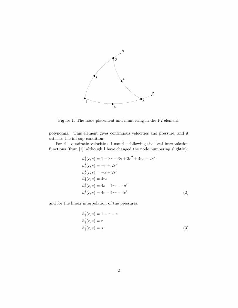
For the finite element solution of the equations (1), I discretize the domainand the solution variables using P2-P1 triangular elements, see figure 1. Thevelocities are represented by the values at the six nodal points per element,and they are interpolated using second degree polynomials. The pressure isrepresented by the three corner nodal values, and interpolated using a linear
1
3
216
5 4
s
r
Figure 1: The node placement and numbering in the P2 element.
polynomial. This element gives continuous velocities and pressure, and itsatisfies the inf-sup condition.
For the quadratic velocities, I use the following six local interpolationfunctions (from [1], although I have changed the node numbering slightly):
hq1(r, s) = 1 − 3r − 3s + 2r2 + 4rs + 2s2
hq2(r, s) = −r + 2r2
hq3(r, s) = −s + 2s2
hq4(r, s) = 4rs
hq5(r, s) = 4s − 4rs − 4s2
hq6(r, s) = 4r − 4rs − 4r2 (2)
and for the linear interpolation of the pressures:
hl1(r, s) = 1 − r − s
hl2(r, s) = r
hl3(r, s) = s. (3)
2

The variables can then be written as functions of the local coordinates:
u(r, s) =6∑
i=1
hqi ui
v(r, s) =6∑
i=1
hqi vi
p(r, s) =3∑
i=1
hlipi (4)
where ui, vi, and pi are the corresponding nodal values. I use isoparametricelements, that is, I interpolate the coordinates with the quadratic interpo-lation functions:
x(r, s) =6∑
i=1
hqi xi (5)
y(r, s) =6∑
i=1
hqi yi (6)
where xi and yi are the coordinates of the node points in the element. Bydifferentiating this, I can form a Jacobian according to
J =[
∂x∂r
∂y∂r
∂x∂s
∂y∂s
](7)
and using this, I can express the derivative operators as[ ∂∂x∂∂y
]= J−1
[∂∂r∂∂s
]. (8)
I then have interpolations for all variables and their derivatives.
2.3 Finite Element Discretization
To obtain the finite element formulation of the equations, I multiply themby virtual velocities u, v and virtual pressures p (interpolated in the same
3
way as the variables), and integrate over the domain:∫V
(− ∂
∂x
(ρν
∂u
∂x
)− ∂
∂y
(ρν
∂u
∂y
)+ ρu
∂u
∂x+ ρv
∂u
∂y+
∂p
∂x
)u dV = 0∫
V
(− ∂
∂x
(ρν
∂v
∂x
)− ∂
∂y
(ρν
∂v
∂y
)+ ρu
∂v
∂x+ ρv
∂v
∂y+
∂p
∂y
)v dV = 0∫
V
(∂u
∂x+
∂v
∂y
)p dV = 0. (9)
Apply the divergence theorem on the diffusive term and set the boundaryintegral to zero (natural boundary conditions):∫
Vρν
(∂u
∂x
∂u
∂x+
∂u
∂y
∂u
∂y
)dV +
∫V
(ρu
∂u
∂x+ ρv
∂u
∂y+
∂p
∂x
)u dV = 0∫
Vρν
(∂v
∂x
∂v
∂x+
∂v
∂y
∂v
∂y
)dV +
∫V
(ρu
∂v
∂x+ ρv
∂v
∂y+
∂p
∂y
)v dV = 0∫
V
(∂u
∂x+
∂v
∂y
)p dV = 0. (10)
Insert the expressions for the interpolated variables and split the integralinto a sum of integrals over the elements, to get a set of discrete nonlinearequations:
L(U) =
Lu(U)Lv(U)Lp(U)
= 0 (11)
where U contains the nodal values of all the degrees of freedom. To solvethis with Newton’s method, I also need to evaluate the tangent stiffnessmatrix (see [1] for details):
K(U) =∂L
∂U=
Kuu(U) Kuv(U) Kup(U)Kvu(U) Kvv(U) Kvp(U)Kpu(U) Kpv(U) 0
(12)
where each submatrix contains the derivative of the corresponding subvectorof L(U). Using this, I can calculate a local stiffness matrix and a localresidual contribution for each element, and with the direct stiffness methodI can insert these result into the global sparse stiffness matrix and into theresidual vector, respectively.
I evaluate all the integrals using a fifth-order, seven points Gauss in-tegration rule. This will integrate all the expressions without integrationerror, since the highest polynomial degree in L(U) is five (from the nonlin-ear convective terms).
4
2.4 Constraint Handling
I impose the boundary constraints by explicitly adding equations and La-grange multipliers. In particular, I extend the solution vector to
Uext =[UΛ
](13)
where Λ are the Lagrange multipliers, and I solve the following extendednonlinear system of equations:
Lext(U,Λ) =[L(U) + NT Λ
NU − M
]= 0 (14)
where the constraints are specified as the linear system of equations NU =M . Similarly, the stiffness matrix is extended according to
Kext(U,Λ) =[K(U) NT
N 0
]. (15)
The Lagrange multipliers Λ can be interpreted as the reactions due to theconstraints.
2.5 Nonlinear Solver
The nonlinear equations are solved by iterating with Newton’s method (Iuse the notations K, L, U below, but the extended matrix and vectors areused):
for i = 1, 2, 3, . . .K(U (i−1))∆U (i) = L(U (i−1))U (i) = U (i−1) + ∆U (i)
end
The routine requires an initial guess U (0), and the iterations are contin-ued until the residual and the correction are small. In particular, I study|L(U (i−1))|∞ and |∆U (i)|∞ in each iteration, and make sure they approachzero.
3 Implementation
In this section, I discuss how I have implemented the code. It is writtenas a Matlab mex-function, which is a way to incorporate external code into
5

the Matlab programming environment. This is convenient, because it allowsme to use Matlab routines for manipulating meshes, doing postprocessing,and calling the linear equations solver. But it also allows for the very highperformance of my optimized C++ code.
My code does all parts of the solution process except mesh generation,solution of linear system of equations, and visualization. In particular, Icreate the data structures for storing the sparse stiffness matrix, I computelocal stiffness matrices for each elements, and I assemble them into the globalsparse matrix. I also include the boundary conditions into this matrix.
3.1 Data Structures
The inputs to my code nsasm.cpp are the mesh, the constraints, the cur-rent solution vector, and the problem parameters according to below. Thenumber of nodes are denoted by np, the number of elements by nt, and thenumber of constrained degrees of freedom by ne.
p - Double precision array with 3×np elements, containing the nodal coor-dinates of the mesh.
t - Integer array with 6×nt elements, containing the indices of the nodesin each element.
np0 - Integer, total number of pressure nodes.
e - Double precision array with 3 × ne elements, containing node number,variables number (0,1, or 2), and value for each constraint.
u - Double precision vector with 2 np+np0+ne elements, containing the cur-rent solution vector.
nu - Double precision, kinematic viscosity.
The outputs are the stiffness matrix (described below) and the residualvector.
3.2 Sparse Matrix Representation
To represent the sparse matrix K, I use the compressed-column format,which is defined as follows. Let nnz be the number of nonzero elementsin the matrix, and let n be the number of columns. The matrix is thenrepresented by the following three arrays:
6
Pr - Double precision vector with nnz elements. Contains the values of eachmatrix entry, in column-wise order starting with the lowest column.
Ir - Integer vector with nnz elements. Contains the row indices for eachmatrix entry.
Jc - Integer vector with n+1 elements. The ith element is an integer spec-ifying the index of the first element in the ith column. In particular,element n+1 is nnz.
The following operations on sparse matrices are implemented:
Creating the matrix. The matrix is created by first counting all the el-ements in each column. Next, the elements are inserted and sortedwithin each column. After this, all duplicate elements can be removed,and finally the three arrays according to above can be formed.
Setting the value of a matrix element. Since the elements in each col-umn are sorted, the position of an element can be extracted using abinary search within the column. The time for this is about the log-arithm of the number of elements in the column, which is boundedindependently of the size of the mesh.
3.3 Subroutines
The code is implemented in C++, and the following subfunctions are used.
init shape Initialize the shape functions in local coordinates. This needsto be done only once, and is extremely fast.
localKL Assemble the K, L contributions from a single element.
sparse create Create a sparse matrix using the algorithm described pre-viously.
sparse set Set the value of an element in the matrix.
assemble Loop over all elements in the mesh, assemble K, L contributionsand insert them into the sparse matrix.
assemble constr Loop over all the constraints NU = M and update theglobal matrix and residual.
The Newton iterations are done with just a few lines of Matlab code:
7
for ii=1:8[K,L]=nsasm(p,t,np0,e,u,nu);du=-lusolve(K,L);u=u+du;disp(sprintf(’%20.10g %20.10g’,norm(L,inf),norm(du,inf)));
end
The disp statement prints the residual and the correction norms. I use thisto determine if the iterations converge or not.
To solve for ∆U (i), I use the SuperLU solver, which is a direct sparsesolver based on Gaussian elimination (see [2] for more details). It uses min-imum degree reordering of the nodes to minimize the fill-in, and it achieveshigh performance by using machine optimized BLAS routines. It is one ofthe fastest direct solvers currently available.
4 Numerical Results
I have studied two common test problems when verifying the results frommy solver. In the first model, I compute the flow around a cylinder in twodimensions. Here I perform “the ultimate” verification test: I solve the sameproblem both in ADINA and with my solver, and compare each entry of thesolution vectors.
In the second test, I simulate the flow inside a closed cavity. By graduallyincreasing the nonlinearities, I can solve the problem for up to Re = 2000.I also study the performance of my solver and look at the sparsity patternof the stiffness matrix.
4.1 Flow around Cylinder
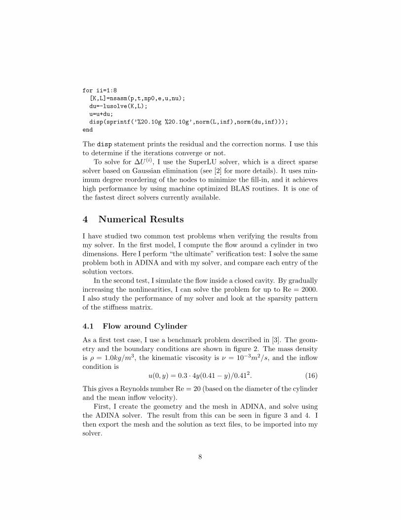
As a first test case, I use a benchmark problem described in [3]. The geom-etry and the boundary conditions are shown in figure 2. The mass densityis ρ = 1.0kg/m3, the kinematic viscosity is ν = 10−3m2/s, and the inflowcondition is
u(0, y) = 0.3 · 4y(0.41 − y)/0.412. (16)
This gives a Reynolds number Re = 20 (based on the diameter of the cylinderand the mean inflow velocity).
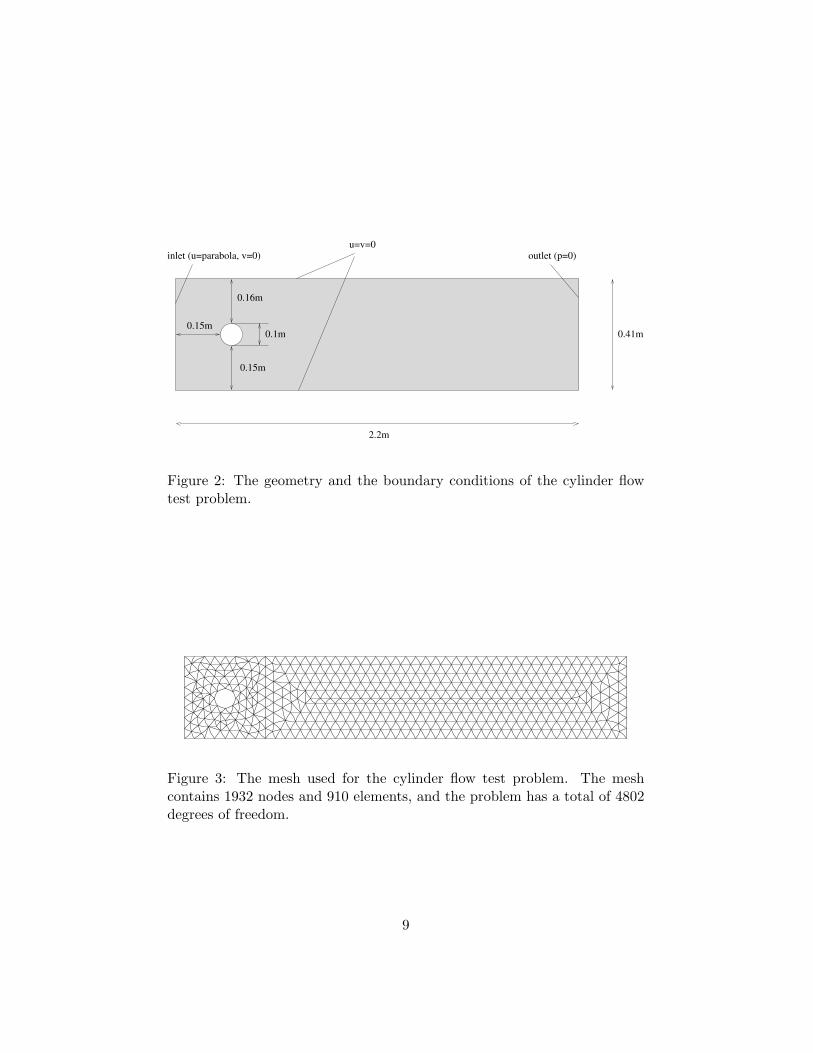
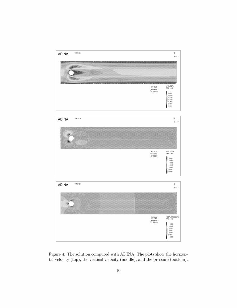
First, I create the geometry and the mesh in ADINA, and solve usingthe ADINA solver. The result from this can be seen in figure 3 and 4. Ithen export the mesh and the solution as text files, to be imported into mysolver.
8
0.15m
2.2m
u=v=0outlet (p=0)inlet (u=parabola, v=0)
0.41m0.1m
0.16m
0.15m
Figure 2: The geometry and the boundary conditions of the cylinder flowtest problem.
Figure 3: The mesh used for the cylinder flow test problem. The meshcontains 1932 nodes and 910 elements, and the problem has a total of 4802degrees of freedom.
9
ADINA TIME 1.000
X Y
Z
Y-VELOCITYTIME 1.000
0.3900
0.3300
0.2700
0.2100
0.1500
0.0900
0.0300
MAXIMUM0.4030
MINIMUM-0.009027
ADINA TIME 1.000
X Y
Z
Z-VELOCITYTIME 1.000
0.1800
0.1200
0.0600
0.0000
-0.0600
-0.1200
-0.1800
MAXIMUM0.2275
MINIMUM-0.2084
ADINA TIME 1.000
X Y
Z
NODAL_PRESSURETIME 1.000
0.1250
0.1000
0.0750
0.0500
0.0250
0.0000
-0.0250
MAXIMUM0.1416
MINIMUM-0.04161
Figure 4: The solution computed with ADINA. The plots show the horizon-tal velocity (top), the vertical velocity (middle), and the pressure (bottom).
10

Iteration Residual |L(U)|∞ Correction |∆U |∞1 0.3 0.39190548922 0.0005369227832 0.18070485613 0.0001834679858 0.029237286654 8.995892913e-06 0.0022146738745 3.005130956e-08 6.152489805e-066 1.064214025e-13 2.838728076e-117 1.682750064e-18 9.540392778e-178 1.950663938e-18 1.02987605e-16
Table 1: The convergence of the Newton iterations on the test problem.The convergence is quadratic, showing that the tangent stiffness matrix iscorrect, and machine precision is obtained after only 7 iterations.
When I run this problem with my solver, I get the residuals and cor-rections according to table 1. Machine precision is achieved in only seveniterations, and the convergence is indeed quadratic as expected with the fullNewton’s method.
I can compare my solution with the solution from ADINA in every node.The result is that the solutions differ by only 5 × 10⁻⁷. This is exactly theerror due to round-off in the ADINA output files, and the two solutions aretherefore essentially identical. This is very good indication that my solveris implemented correctly.
Another verification of the result can be made by comparing the quan-tities discussed in [3]. I compute two of these:
Pressure difference across cylinder. The difference ∆p = p(0.15, 0.15)−p(0.25, 0.15) can be computed by simply subtracting the nodal pres-sure values at the corresponding points.
Length of recirculation region. There is a recirculation region behindthe cylinder, and the length of it can be calculated by finding theposition where u = 0 and subtracting 0.25.
In table 2, the convergence of these two quantities is shown, together withan interval of expected values. For the two finest meshes, both results arewithin these intervals.
I can now try to decrease the viscosity to see how large Reynold’s num-bers my solver can handle for this problem. There are (at least) three reasonsthat my solver is insufficient for high Reynold’s numbers:
11
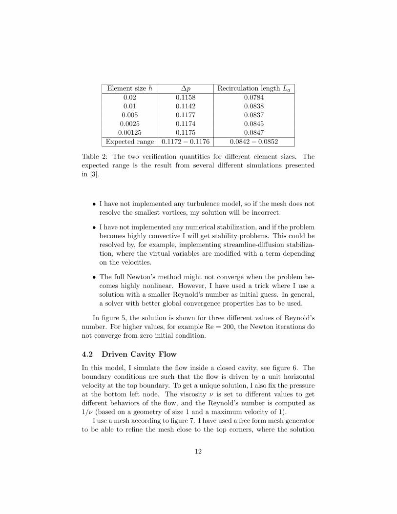
Element size h ∆p Recirculation length La
0.02 0.1158 0.07840.01 0.1142 0.08380.005 0.1177 0.08370.0025 0.1174 0.08450.00125 0.1175 0.0847
Expected range 0.1172 − 0.1176 0.0842 − 0.0852
Table 2: The two verification quantities for different element sizes. Theexpected range is the result from several different simulations presentedin [3].
• I have not implemented any turbulence model, so if the mesh does notresolve the smallest vortices, my solution will be incorrect.
• I have not implemented any numerical stabilization, and if the problembecomes highly convective I will get stability problems. This could beresolved by, for example, implementing streamline-diffusion stabiliza-tion, where the virtual variables are modified with a term dependingon the velocities.
• The full Newton’s method might not converge when the problem be-comes highly nonlinear. However, I have used a trick where I use asolution with a smaller Reynold’s number as initial guess. In general,a solver with better global convergence properties has to be used.
In figure 5, the solution is shown for three different values of Reynold’snumber. For higher values, for example Re = 200, the Newton iterations donot converge from zero initial condition.
4.2 Driven Cavity Flow
In this model, I simulate the flow inside a closed cavity, see figure 6. Theboundary conditions are such that the flow is driven by a unit horizontalvelocity at the top boundary. To get a unique solution, I also fix the pressureat the bottom left node. The viscosity ν is set to different values to getdifferent behaviors of the flow, and the Reynold’s number is computed as1/ν (based on a geometry of size 1 and a maximum velocity of 1).
I use a mesh according to figure 7. I have used a free form mesh generatorto be able to refine the mesh close to the top corners, where the solution
12

Figure 5: The solution to the flow around cylinder problem, for Re = 20(top), Re = 60 (middle), and Re = 100 (bottom). The magnitude of thevelocity is shown.
13

u=1, v=0
u=v=0
u=v=0
u=v=0
p=0 1
1
Figure 6: The geometry and the boundary conditions of the driven cavityflow test problem.
has singularities. I have solved the problem for four different Reynold’snumbers: 100, 500, 1000, and 2000. For the highest values, I had to usethe previous solutions in order to converge in the Newton iterations. Theresults are shown in figure 8.
4.3 Performance
I have tried to optimize my code as much as possible, and the result is thatthe time for creating the sparse matrix data structures and assemble thestiffness matrix is completely negligible compared to the time for solvingthe linear system of equations. For instance, a problem with 15794 nodes,7754 elements, and 36692 degrees of freedom (a relatively large problem)requires about 1 second in my routine on a Pentium 4 computer, while thetime spent in SuperLU is about 30 seconds. In total, it takes a few minutesto obtain the solution in about 6 iterations.
It is interesting to investigate the sparsity pattern of the stiffness matrix.In figure 9, it is shown for the mesh used in the cylinder flow example.One can clearly see the different parts of the stiffness matrix, including theconstraints and the Lagrange multipliers. The number of nonzero entries is125419, giving an average of about 26 elements per column.
14

Figure 7: The mesh used in the driven cavity example. The mesh is refinedat the top corners and at the top boundary to resolve the singularities. Themesh contains 3581 nodes and 1722 elements, and the problem has a totalof 8637 degrees of freedom.
References
[1] Klaus-Jurgen Bathe. Finite Element Procedures. Prentice Hall, 1996.
[2] James W. Demmel, John R. Gilbert, and Xiaoye S. Li. SuperLU Users’Guide, September 1999.
[3] M. Schafer and S. Turek. Benchmark computations of laminar flowaround a cylinder. Notes on Numerical Fluid Mechanics, 52:547–566,1996.
15

Re = 100 Re = 500
Re = 1000 Re = 2000
Figure 8: The solution to the driven cavity problem for four differentReynold’s numbers. The contours of the magnitude of the velocity areshown.
16
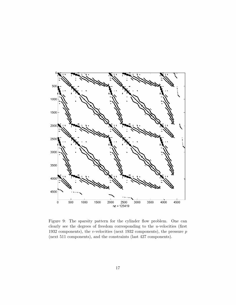
Figure 9: The sparsity pattern for the cylinder flow problem. One canclearly see the degrees of freedom corresponding to the u-velocities (first1932 components), the v-velocities (next 1932 components), the pressure p(next 511 components), and the constraints (last 427 components).
17
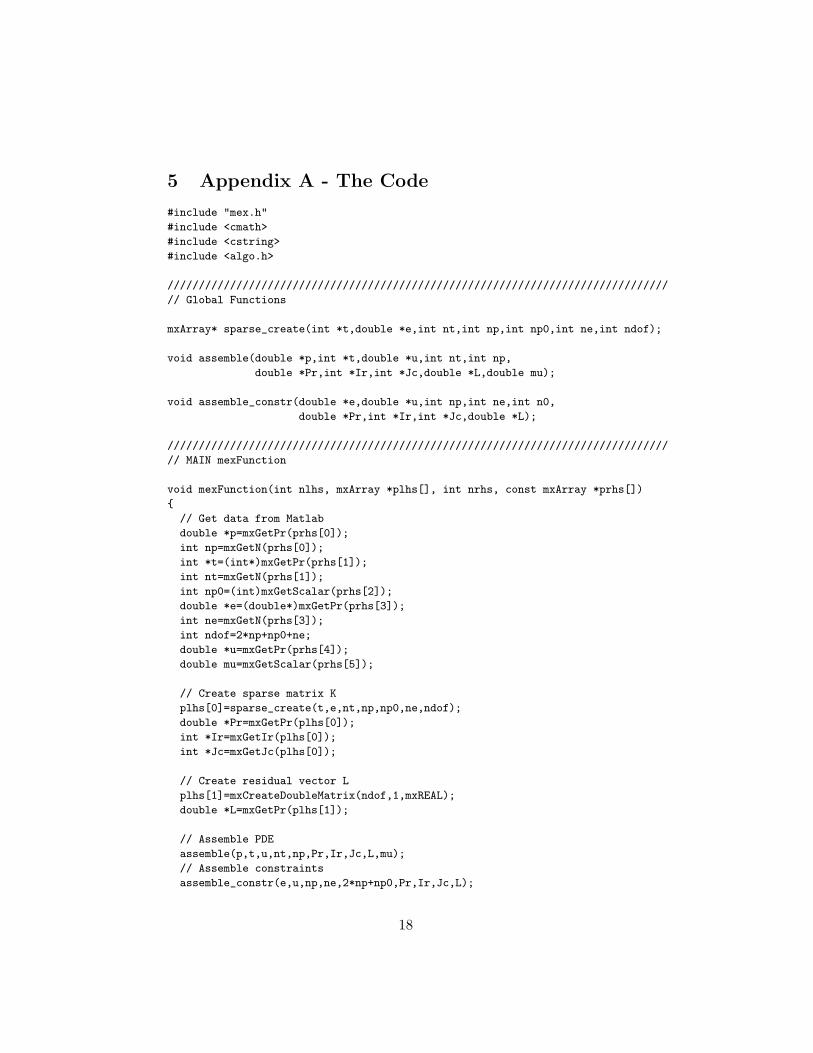
5 Appendix A - The Code
#include "mex.h"
#include <cmath>
#include <cstring>
#include <algo.h>
////////////////////////////////////////////////////////////////////////////////
// Global Functions
mxArray* sparse_create(int *t,double *e,int nt,int np,int np0,int ne,int ndof);
void assemble(double *p,int *t,double *u,int nt,int np,
double *Pr,int *Ir,int *Jc,double *L,double mu);
void assemble_constr(double *e,double *u,int np,int ne,int n0,
double *Pr,int *Ir,int *Jc,double *L);
////////////////////////////////////////////////////////////////////////////////
// MAIN mexFunction
void mexFunction(int nlhs, mxArray *plhs[], int nrhs, const mxArray *prhs[])
{
// Get data from Matlab
double *p=mxGetPr(prhs[0]);
int np=mxGetN(prhs[0]);
int *t=(int*)mxGetPr(prhs[1]);
int nt=mxGetN(prhs[1]);
int np0=(int)mxGetScalar(prhs[2]);
double *e=(double*)mxGetPr(prhs[3]);
int ne=mxGetN(prhs[3]);
int ndof=2*np+np0+ne;
double *u=mxGetPr(prhs[4]);
double mu=mxGetScalar(prhs[5]);
// Create sparse matrix K
plhs[0]=sparse_create(t,e,nt,np,np0,ne,ndof);
double *Pr=mxGetPr(plhs[0]);
int *Ir=mxGetIr(plhs[0]);
int *Jc=mxGetJc(plhs[0]);
// Create residual vector L
plhs[1]=mxCreateDoubleMatrix(ndof,1,mxREAL);
double *L=mxGetPr(plhs[1]);
// Assemble PDE
assemble(p,t,u,nt,np,Pr,Ir,Jc,L,mu);
// Assemble constraints
assemble_constr(e,u,np,ne,2*np+np0,Pr,Ir,Jc,L);
18
}
////////////////////////////////////////////////////////////////////////////////
// Gauss integration
// Number of Gauss points
const int ngp=7;
// GP data
const double w1=0.225000000000000;
const double w2=0.132394152788506;
const double w3=0.125939180544827;
const double a1=0.333333333333333;
const double a2=0.059715871789770;
const double a3=0.797426985353087;
const double b2=(1-a2)/2;
const double b3=(1-a3)/2;
// Gauss points
static double gp[ngp][3]={a1,a1,1-a1-a1,
a2,b2,1-a2-b2,
b2,a2,1-b2-a2,
b2,b2,1-b2-b2,
a3,b3,1-a3-b3,
b3,a3,1-b3-a3,
b3,b3,1-b3-b3};
// Gauss weights
static double w[ngp]={w1,w2,w2,w2,w3,w3,w3};
////////////////////////////////////////////////////////////////////////////////
// Global data
static double sh1[ngp][3]; // P1 Shape functions
static double sh1r[ngp][3]; // P1 Shape functions r-derivatives
static double sh1s[ngp][3]; // P1 Shape functions s-derivatives
static double sh2[ngp][6]; // P2 Shape functions
static double sh2r[ngp][6]; // P2 Shape functions r-derivatives
static double sh2s[ngp][6]; // P2 Shape functions s-derivatives
////////////////////////////////////////////////////////////////////////////////
// init_shape
void init_shape()
{
for (int i=0; i<ngp; i++) {
// P1 Shape functions
sh1[i][0]=gp[i][2];
sh1[i][1]=gp[i][0];
19
sh1[i][2]=gp[i][1];
// P1 Shape functions r-derivatives
sh1r[i][0]=-1;
sh1r[i][1]=1;
sh1r[i][2]=0;
// P1 Shape functions s-derivatives
sh1s[i][0]=-1;
sh1s[i][1]=0;
sh1s[i][2]=1;
// P2 Shape functions
sh2[i][0]=1-3*gp[i][0]-3*gp[i][1]+2*gp[i][0]*gp[i][0]+
4*gp[i][0]*gp[i][1]+2*gp[i][1]*gp[i][1];
sh2[i][1]=-gp[i][0]+2*gp[i][0]*gp[i][0];
sh2[i][2]=-gp[i][1]+2*gp[i][1]*gp[i][1];
sh2[i][3]=4*gp[i][0]*gp[i][1];
sh2[i][4]=4*gp[i][1]-4*gp[i][0]*gp[i][1]-4*gp[i][1]*gp[i][1];
sh2[i][5]=4*gp[i][0]-4*gp[i][0]*gp[i][1]-4*gp[i][0]*gp[i][0];
// P2 Shape functions r-derivatives
sh2r[i][0]=-3+4*gp[i][0]+4*gp[i][1];
sh2r[i][1]=-1+4*gp[i][0];
sh2r[i][2]=0;
sh2r[i][3]=4*gp[i][1];
sh2r[i][4]=-4*gp[i][1];
sh2r[i][5]=4-8*gp[i][0]-4*gp[i][1];
// P2 Shape functions s-derivatives
sh2s[i][0]=-3+4*gp[i][0]+4*gp[i][1];
sh2s[i][1]=0;
sh2s[i][2]=-1+4*gp[i][1];
sh2s[i][3]=4*gp[i][0];
sh2s[i][4]=4-8*gp[i][1]-4*gp[i][0];
sh2s[i][5]=-4*gp[i][0];
}
}
////////////////////////////////////////////////////////////////////////////////
// localKL
void localKL(double *p,int *tt,double *u0,int np,double lK[15][15],double lL[15],double mu)
{
memset(lK,0,15*15*sizeof(double));
memset(lL,0,15*sizeof(double));
for (int igp=0; igp<ngp; igp++) {
// Jacobian
double xr,xs,yr,ys;
xr=xs=yr=ys=0.0;
for (int i=0; i<6; i++) {
xr+=sh2r[igp][i]*p[(tt[i]-1)*2+0];
xs+=sh2s[igp][i]*p[(tt[i]-1)*2+0];
20
yr+=sh2r[igp][i]*p[(tt[i]-1)*2+1];
ys+=sh2s[igp][i]*p[(tt[i]-1)*2+1];
}
double Jdet=xr*ys-xs*yr;
double Jinv[2][2]={ys/Jdet,-xs/Jdet,-yr/Jdet,xr/Jdet};
// x,y derivatives of shape functions
double sh1x[3],sh1y[3],sh2x[6],sh2y[6];
for (int i=0; i<3; i++) {
sh1x[i]=sh1r[igp][i]*Jinv[0][0]+sh1s[igp][i]*Jinv[1][0];
sh1y[i]=sh1r[igp][i]*Jinv[0][1]+sh1s[igp][i]*Jinv[1][1];
}
for (int i=0; i<6; i++) {
sh2x[i]=sh2r[igp][i]*Jinv[0][0]+sh2s[igp][i]*Jinv[1][0];
sh2y[i]=sh2r[igp][i]*Jinv[0][1]+sh2s[igp][i]*Jinv[1][1];
}
// Solution and derivatives
double u,ux,uy,v,vx,vy;
u=ux=uy=v=vx=vy=0.0;
for (int i=0; i<6; i++) {
u+=sh2[igp][i]*u0[tt[i]-1];
ux+=sh2x[i]*u0[tt[i]-1];
uy+=sh2y[i]*u0[tt[i]-1];
v+=sh2[igp][i]*u0[np+tt[i]-1];
vx+=sh2x[i]*u0[np+tt[i]-1];
vy+=sh2y[i]*u0[np+tt[i]-1];
}
double px,py;
px=py=0.0;
for (int i=0; i<3; i++) {
px+=sh1x[i]*u0[2*np+tt[i]-1];
py+=sh1y[i]*u0[2*np+tt[i]-1];
}
// Local K and L
double mul=w[igp]*Jdet/2.0;
for (int i=0; i<6; i++) {
lL[i]+=(u*ux+v*uy+px)*sh2[igp][i]*mul;
lL[6+i]+=(u*vx+v*vy+py)*sh2[igp][i]*mul;
lL[i]+=mu*(ux*sh2x[i]+uy*sh2y[i])*mul;
lL[6+i]+=mu*(vx*sh2x[i]+vy*sh2y[i])*mul;
for (int j=0; j<6; j++) {
lK[i][j]+=mu*(sh2x[i]*sh2x[j]+sh2y[i]*sh2y[j])*mul;
lK[6+i][6+j]+=mu*(sh2x[i]*sh2x[j]+sh2y[i]*sh2y[j])*mul;
lK[i][j]+=(u*sh2[igp][i]*sh2x[j]+v*sh2[igp][i]*sh2y[j])*mul;
lK[6+i][6+j]+=(u*sh2[igp][i]*sh2x[j]+v*sh2[igp][i]*sh2y[j])*mul;
lK[i][j]+=(ux*sh2[igp][i]*sh2[igp][j])*mul;
lK[i][6+j]+=(uy*sh2[igp][i]*sh2[igp][j])*mul;
21

lK[6+i][j]+=(vx*sh2[igp][i]*sh2[igp][j])*mul;
lK[6+i][6+j]+=(vy*sh2[igp][i]*sh2[igp][j])*mul;
}
for (int j=0; j<3; j++) {
lK[i][12+j]+=(sh2[igp][i]*sh1x[j])*mul;
lK[6+i][12+j]+=(sh2[igp][i]*sh1y[j])*mul;
}
}
for (int i=0; i<3; i++) {
lL[12+i]+=(ux+vy)*sh1[igp][i]*mul;
for (int j=0; j<6; j++) {
lK[12+i][j]+=(sh1[igp][i]*sh2x[j])*mul;
lK[12+i][6+j]+=(sh1[igp][i]*sh2y[j])*mul;
}
}
}
}
////////////////////////////////////////////////////////////////////////////////
// sparse_create
mxArray* sparse_create(int *t,double *e,int nt,int np,int np0,int ne,int ndof)
{
int *idxi,*idxj;
int nidx=nt*15*15+2*ne; // Upper limit on # entries
idxi=(int*)mxCalloc(nidx,sizeof(int)); // Row indices
idxj=(int*)mxCalloc(nidx,sizeof(int)); // Column indices
int *col=(int*)mxCalloc(ndof,sizeof(int)); // # entries in each column
int *colstart=(int*)mxCalloc(ndof,sizeof(int)); // start index of each column
int ie;
double *n;
// Count elements in each columns (including duplicates)
for (int it=0,*n=t; it<nt; it++,n+=6) {
for (int j=0; j<6; j++) {
col[n[j]-1]+=15;
col[n[j]-1+np]+=15;
}
for (int j=0; j<3; j++) {
col[n[j]-1+2*np]+=15;
}
}
// Constraints
for (ie=0,n=e; ie<ne; ie++,n+=3) {
col[2*np+np0+ie]++;
col[(int)n[1]*np+(int)n[0]-1]++;
}
22

// Form cumulative sum (start of each column)
for (int i=0; i<ndof-1; i++)
colstart[i+1]=colstart[i]+col[i];
// Insert row/column indices, sorted columns
for (int it=0,*n=t; it<nt; it++,n+=6) {
for (int i=0; i<15; i++) {
int ri=n[i%6]+np*(i/6)-1;
for (int j=0; j<15; j++) {
int rj=n[j%6]+np*(j/6)-1;
idxi[colstart[rj]]=ri;
idxj[colstart[rj]]=rj;
colstart[rj]++;
}
}
}
// Constraints
for (ie=0,n=e; ie<ne; ie++,n+=3) {
int ri,rj;
ri=(int)n[1]*np+(int)n[0]-1;
rj=2*np+np0+ie;
idxi[colstart[rj]]=ri;
idxj[colstart[rj]]=rj;
colstart[rj]++;
ri=2*np+np0+ie;
rj=(int)n[1]*np+(int)n[0]-1;
idxi[colstart[rj]]=ri;
idxj[colstart[rj]]=rj;
colstart[rj]++;
}
mxFree(colstart);
// Sort row indices in each column
int *p=idxi;
for (int i=0; i<ndof; i++) {
sort(p,p+col[i]);
p+=col[i];
}
// Count unique entries
memset(col,0,ndof*sizeof(int));
int nnz=1; col[idxj[0]]++;
for (int ii=1; ii<nidx; ii++) {
if (idxi[ii]!=idxi[ii-1] ||
idxj[ii]!=idxj[ii-1]) {
nnz++;
23

col[idxj[ii]]++;
}
}
// Create sparse matrix
mxArray *K=mxCreateSparse(ndof,ndof,nnz,mxREAL);
int *Ir=mxGetIr(K);
int *Jc=mxGetJc(K);
// Form Jc vector
Jc[0]=0;
for (int i=1; i<=ndof; i++)
Jc[i]=Jc[i-1]+col[i-1];
mxFree(col);
// Form Ir vector
*(Ir++)=idxi[0];
for (int ii=1; ii<nidx; ii++)
if (idxi[ii]!=idxi[ii-1] ||
idxj[ii]!=idxj[ii-1])
*(Ir++)=idxi[ii];
mxFree(idxj);
mxFree(idxi);
return K;
}
////////////////////////////////////////////////////////////////////////////////
// sparse_set
void sparse_set(double *Pr,int *Ir,int *Jc,int ri,int rj,double val)
{
// Binary search within column
int k,k1,k2,cr=ri;
k1=Jc[rj];
k2=Jc[rj+1]-1;
do {
k=(k1+k2)>>1;
if (cr<Ir[k])
k2=k-1;
else
k1=k+1;
if (cr==Ir[k])
break;
} while (k2>=k1);
Pr[k]+=val;
}
24

////////////////////////////////////////////////////////////////////////////////
// assemble
void assemble(double *p,int *t,double *u,int nt,int np,
double *Pr,int *Ir,int *Jc,double *L,double mu)
{
init_shape();
double lK[15][15];
double lL[15];
for (int it=0,*n=t; it<nt; it++,n+=6) {
localKL(p,n,u,np,lK,lL,mu);
for (int i=0; i<15; i++) {
int ri=n[i%6]+np*(i/6)-1;
L[ri]+=lL[i];
for (int j=0; j<15; j++) {
int rj=n[j%6]+np*(j/6)-1;
sparse_set(Pr,Ir,Jc,ri,rj,lK[i][j]);
}
}
}
}
////////////////////////////////////////////////////////////////////////////////
// assemble_constr
void assemble_constr(double *e,double *u,int np,int ne,int n0,
double *Pr,int *Ir,int *Jc,double *L)
{
int ie;
double *n;
for (ie=0,n=e; ie<ne; ie++,n+=3) {
int ri=n0+ie;
int rj=(int)n[1]*np+(int)n[0]-1;
sparse_set(Pr,Ir,Jc,ri,rj,1.0);
sparse_set(Pr,Ir,Jc,rj,ri,1.0);
L[rj]+=u[ri];
L[ri]=u[rj]-n[2];
}
}
////////////////////////////////////////////////////////////////////////////////
// END
////////////////////////////////////////////////////////////////////////////////
25


