Md. Nafiul Haque (Ph.D. Candidate) Murad Y. Abu-Farsakh, Ph.D., P.E. Louisiana Transportation Conference March 1, 2016 Implementation of Pile Setup in the LRFD Design of Driven Piles in Louisiana
Transcript
Md. Nafiul Haque (Ph.D. Candidate)
Murad Y. Abu-Farsakh, Ph.D., P.E.
Louisiana Transportation Conference March 1, 2016
Implementation of Pile Setup in
the LRFD Design of Driven Piles
in Louisiana
OUTLINE
Objectives
Brief Background
Methodology
Results and Analysis
Analytical Models
LRFD Calibration
2
OBJECTIVES
Evaluate the time-dependant increase in pile capacity
(or setup) for piles driven into Louisiana soils through
conducting repeated static and dynamic field testing
with time on full-scale instrumented test piles.
Study the effect of soil type/properties, pile size, and
their interaction on pile setup phenomenon.
Develop analytical model(s) to estimate pile setup with
time using typical soil properties.
Incorporate setup into LRFD design of driven pile in
Pile resistance/capacity have been reported to usually increase with time, after end of pile driving (EOD). The increase in resistance/capacity after end of driving, is known as pile set-up. Set-up is observed both in cohesive (clayey) and non-cohesive (sandy-silty) soils.
4
Benefits of Incorporating Set-up in Design
The implementation of pile set-up capacity in the design can result in significant cost savings through
Shortening pile lengths
Reducing pile cross-sectional area (using smaller-diameter/width piles)
Smaller hammer to drive pile
Reducing the number of piles Substantial cost will be saved for full project
5
MECHANISMS - Pile Set-Up
Soil around the pile usually experiences plastic deformation
and remolded during pile driving. Excess pore water pressure
develops as the result of pile driving.
After the completion of pile driving, a certain degree of excess pore water pressure dissipates at the soil-pile interface zone, usually resulting in an increase in pile resistance.
“Aging” and “Thixotropy” also plays significant role in set-up.
Fellenius, 2008
Result from Our Study 6
MECHANISMS - Pile Set-Up In cohesive soils, the induced excess pore water pressure may dissipate
slowly due to low permeability and it takes 50-100 days to dissipate.
However, for noncohesive soils, the duration of dissipation of excess pore
water pressure take several hours to several days due to high
permeability.
This dissipation phase plays the most significant role for the set-up
phase / period or how long it will take for the completion of set-up.
Sandy Soil Clayey Soil
7
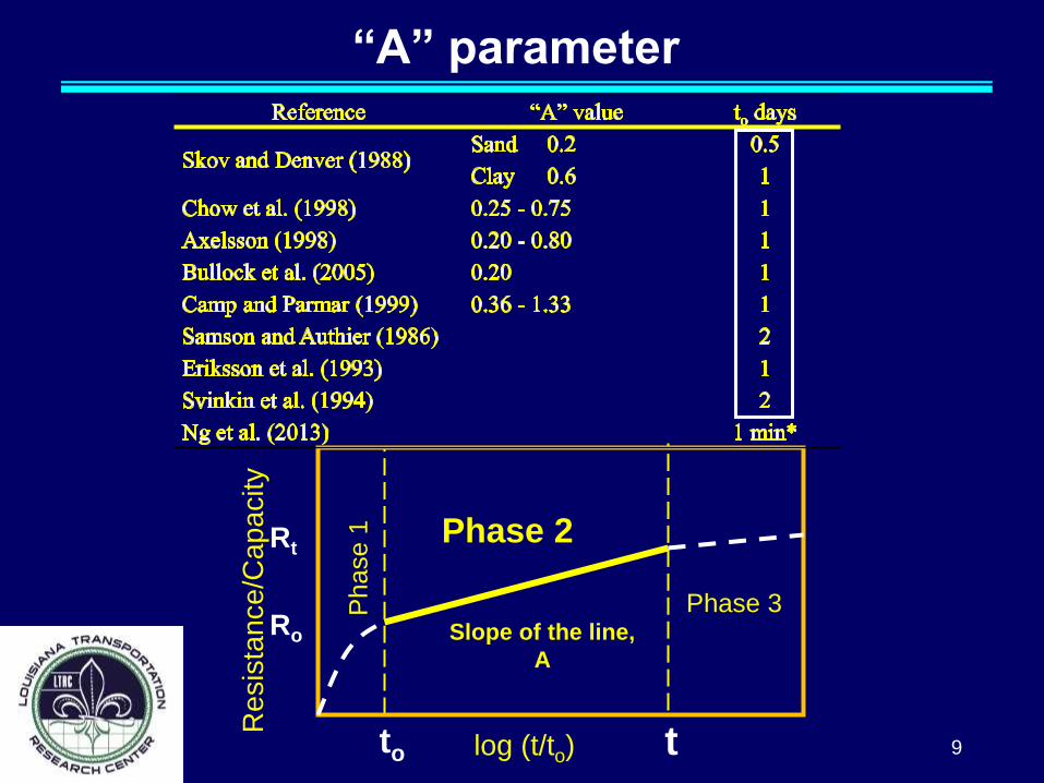
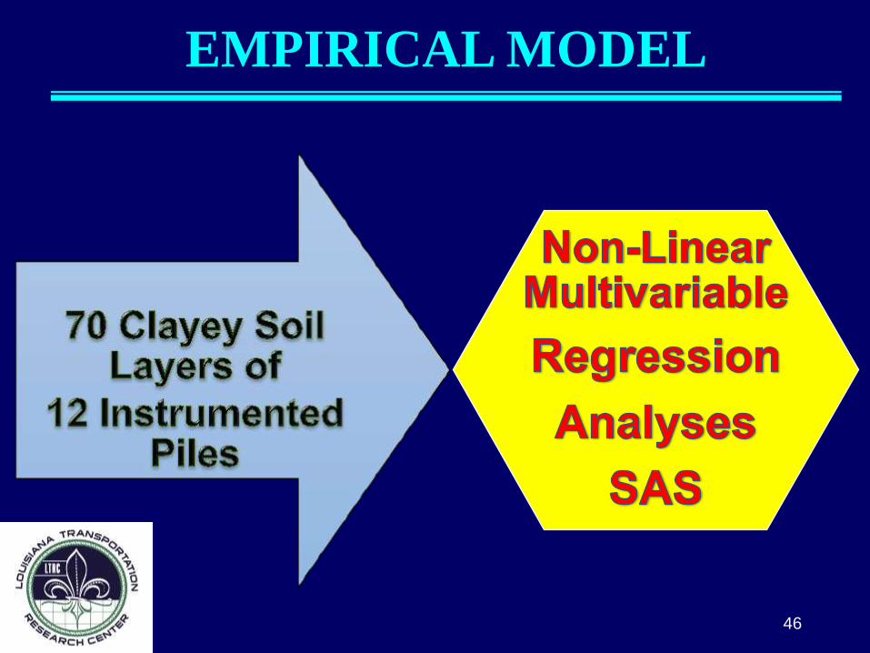
EMPIRICAL MODELS
The model that were developed earlier were mainly formed by regression analyses of limited data sets. The first model for pile set-up was proposed by Skov and Denver in 1988.
𝐑
𝐭
𝐑𝐨
= 1 + A log10 𝐭
𝐭𝐨
Rt: the ultimate pile capacity at time t after driving,
Ro: the ultimate pile capacity at time (Reference time) to, A : a constant that depends on soil type and pile
characteristics,
to: initial time (taken as the time to first restrike), Reference time
8
“A” parameter
9 log (t/to)
Phase 2
Phase 3 Phase 1
Re
sis
tan
ce
/Cap
acity
to t
Ro
Rt
Slope of the line,
A
Methodology
10
Conduct
Field Test
Collect Data From Performed
Old Set-up Studies
Analyze Data For Individual Soil
Layers
Correlate Set-up of Individual Soil Layers with Soil
Properties
Develop
Model
LRFD Calibration
Field
Projects
Instrumented Test Piles
(12 Test Piles)
METHODOLOGY
11
1.Bayou Lacassine (3 Test Piles)
2.Bayou Zourie (1 Test Pile)
3.Bayou Bouef (1 Test Pile)
4.LA-1 (6 Test Piles)
5.Bayou Teche (1 Test Pile)
12
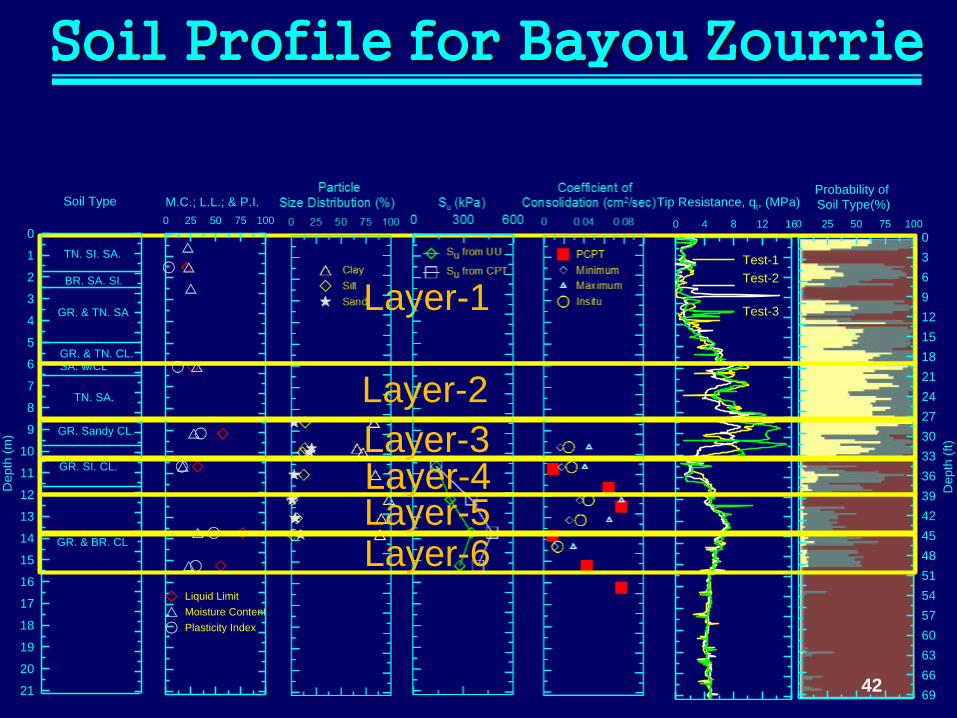
METHODOLOGY-FIELD PROJECTS
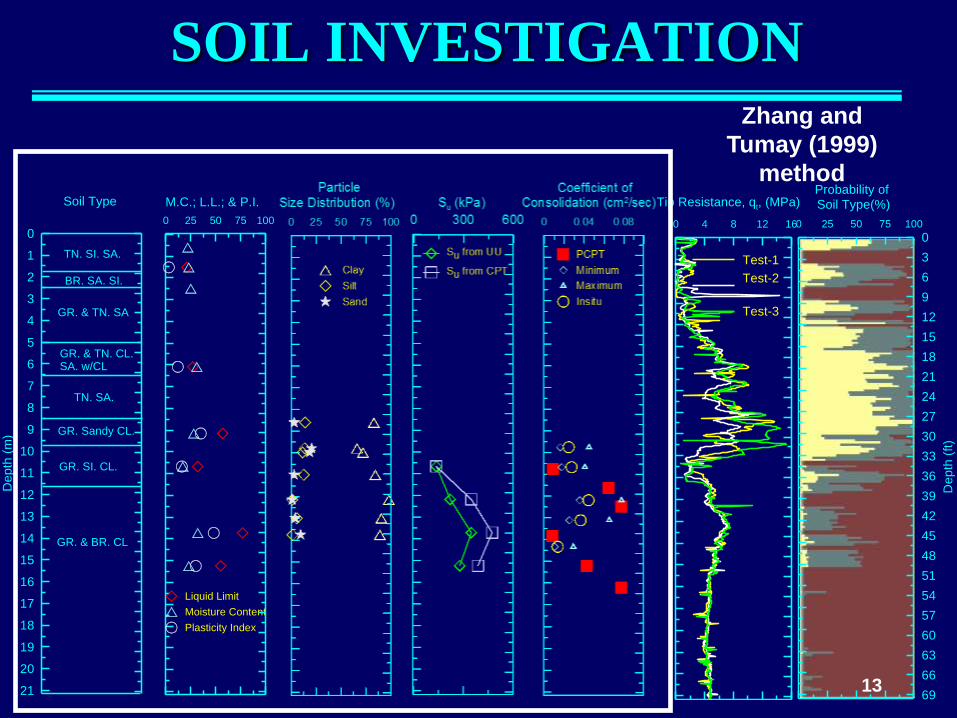
SOIL INVESTIGATION
Test-1
Test-2
Test-3
0 4 8 12 16
Tip Resistance, qt, (MPa)
0
3
6
9
12
15
18
21
24
27
30
33
36
39
42
45
48
51
54
57
60
63
66
69
De
pth
(ft)
0 25 50 75 100
Probability of
Soil Type(%)
TN. SI. SA.
21
20
19
18
17
16
15
14
13
12
11
10
9
8
7
6
5
4
3
2
1
0
De
pth
(m
)
Soil Type
GR. & TN. SA
GR. & TN. CL.SA. w/CL
BR. SA. SI.
Liquid Limit
Moisture Content
Plasticity Index
0 25 50 75 100
M.C.; L.L.; & P.I.
Clay
Silt
Sand
0 25 50 75 100
Particle
Size Distribution (%)
Su from UU
Su from CPT
0 300 600
Su (kPa)
TN. SA.
GR. & BR. CL
GR. SI. CL.
PCPT
Minimum
Maximum
Insitu
0 0.04 0.08
Coefficient of
Consolidation (cm2/sec)
GR. Sandy CL.
13
Zhang and
Tumay (1999)
method
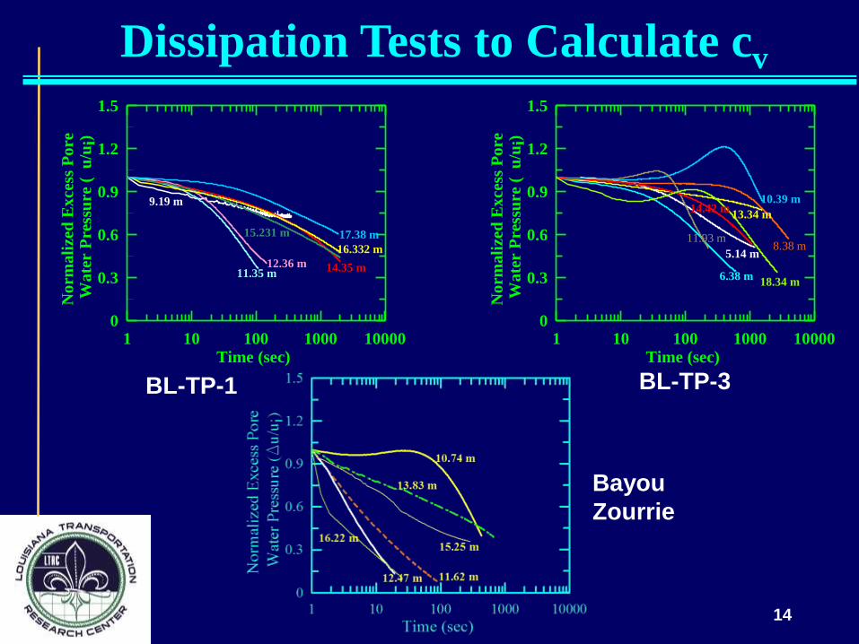
Dissipation Tests to Calculate cv
1 10 100 1000 10000Time (sec)
0
0.3
0.6
0.9
1.2
1.5
No
rmali
zed
Ex
ces
s P
ore
W
ate
r P
ress
ure
( u
/ui)
12.36 m
17.38 m
14.35 m
15.231 m
16.332 m
9.19 m
11.35 m
BL-TP-1
1 10 100 1000 10000Time (sec)
0
0.3
0.6
0.9
1.2
1.5
No
rmali
zed
Ex
ces
s P
ore
W
ate
r P
ress
ure
( u
/ui)
13.34 m
11.93 m8.38 m
18.34 m
5.14 m
6.38 m
14.42 m10.39 m
BL-TP-3
Bayou
Zourrie
14
METHODOLOGY-INSTRUMENTATION
Sister bar Strain gauges Pressure cells Piezometers Multilevel Piezometers
Soil Profile 15
Sandy
Clayey
Clayey
Clayey
Sandy
Sandy
Cv from Lab
Cv from PCPT
1E-005 0.001 0.1
Coefficient of
Consolidation (cm2/sec)
0 25 50 75 100
M.C.; L.L; & P.I.
.Su from UU
Su from CPT
0 100 200 300
Su (kPa)
Liquid Limit
Plasticity Index
Moisture Content
BR & Light Gr., Organic Clay, OH
Light Br.,Silty Clay, CL
21
20
19
18
17
16
15
14
13
12
11
10
9
8
7
6
5
4
3
2
1
0
De
pth
(m
)
Soil Type
Light Gr.,Organic Clay, OH
Gr., Silty Clay CL
Dark Gr.,Silty Clay, CL
Gr., Lean Clay CL
Reddish Light Br.,SIlty Clay, CL
Light Br.,Sandy Clay, CH
Light Br., Silty Clay, CL
Dark Gr.,Sandy Clay, CL
OCR from CPT
OCR from Lab
0 1 2 3 4 5
OCR
0 4 8 12
Tip
Resistance, qt (MPa)
0 5 10 15 20 25
Rf (%)
69
65
62
59
56
52
49
46
43
39
36
33
29
26
23
20
16
13
10
7
3
0
De
pth
(ft
)
0 25 50 75 100
Probability of
Soil Type (%)
Casing
30"
21.0'
11.0'
5.0'
5.0'
10.0'
5.0'
28.0'
12.0'
14.0'
10.0'
5.0'
5.0'
B B B
B
B
B
B
B
B
G.L.
8.0'
MP-7 MP-8 MP-9
MP-4 MP-5 MP-6
MP-1 MP-2 MP-3
Layer-8
Layer-7
Layer-6
Layer-5
Layer-4
Layer-3
Layer-2
Layer-1
Sandy
Clayey
Clayey
Clayey
Always one pair of strain
gauge was installed near top
in order to calibrate the elastic
modulus
One pair of strain gauge near
tip in order to calculate the tip
resistance
16
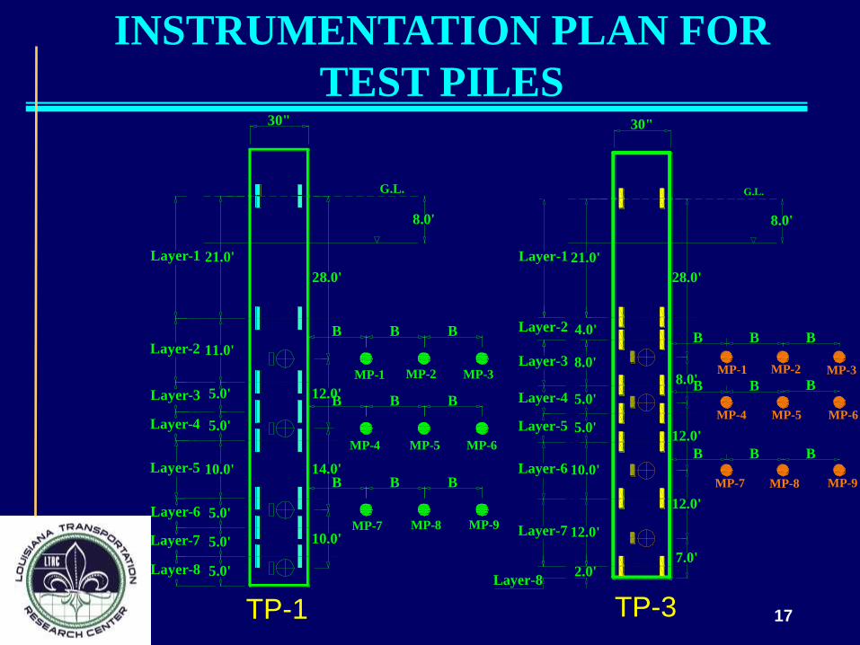
METHODOLOGY-INSTRUMENTATION
INSTRUMENTATION PLAN FOR
TEST PILES 30"
21.0'
11.0'
5.0'
5.0'
10.0'
5.0'
28.0'
12.0'
14.0'
10.0'
5.0'
5.0'
B B B
B
B
B
B
B
B
G.L.
8.0'
MP-7 MP-8 MP-9
MP-4 MP-5 MP-6
MP-1 MP-2 MP-3
Layer-8
Layer-7
Layer-6
Layer-5
Layer-4
Layer-3
Layer-2
Layer-1
TP-1
30"
21.0'
4.0'
8.0'
5.0'
5.0'
10.0'
12.0'
7.0'
8.0'
12.0'
12.0'
28.0'
8.0'
G.L.
B B B
B
B
B
B
B
B
MP-7 MP-8 MP-9
MP-4 MP-5 MP-6
MP-1 MP-2 MP-3
Layer-7
Layer-6
Layer-5
Layer-4
Layer-3
Layer-2
Layer-1
Layer-82.0'
TP-3 17
Sister bar strain
gauges Sister bar strain gauges always
installed in pairs-
The average readings were taken
in order to eliminate the effect
bending stress during driving
18
INSTRUMENTATION
Pressure cell
Piezometer
Pressure cell & Piezometer
Geokon Model 4820
Geokon Model 4500S
19
INSTRUMENTATION
Before
Pouring
Concrete
After
Pouring
Concrete
Installed in
predefined
depth
20
INSTRUMENTATION
Saturated
before
driving
Vacuum pump and
peanut oil was used
21
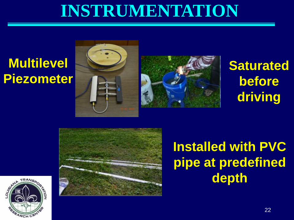
INSTRUMENTATION
Saturated
before
driving
Multilevel
Piezometer
Installed with PVC
pipe at predefined
depth
22
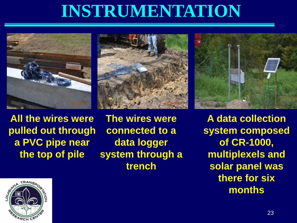
INSTRUMENTATION
INSTRUMENTATION
A data collection
system composed
of CR-1000,
multiplexels and
solar panel was
there for six
months
All the wires were
pulled out through
a PVC pipe near
the top of pile
The wires were
connected to a
data logger
system through a
trench
23
DRIVING AND LOAD TESTS
Hammer
Accelerometer
and strain
transducer PDA
device
24
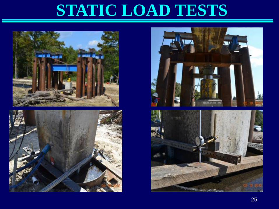
STATIC LOAD TESTS
25
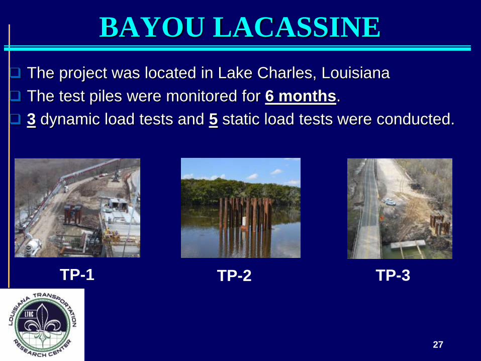
BAYOU LACASSINE
26
The project was located in Lake Charles, Louisiana
The test piles were monitored for 6 months.
3 dynamic load tests and 5 static load tests were conducted.
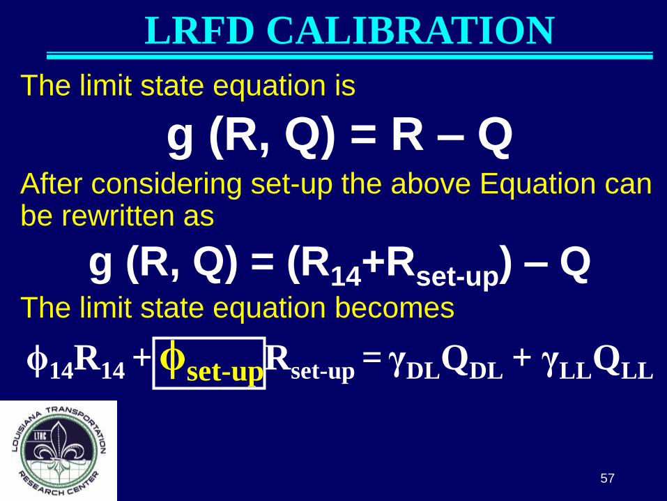
g (R, Q) = R – Q After considering set-up the above Equation can be rewritten as
g (R, Q) = (R14+Rset-up) – Q The limit state equation becomes
ϕ14R14 + ϕset-upRset-up = γDLQDL + γLLQLL
57
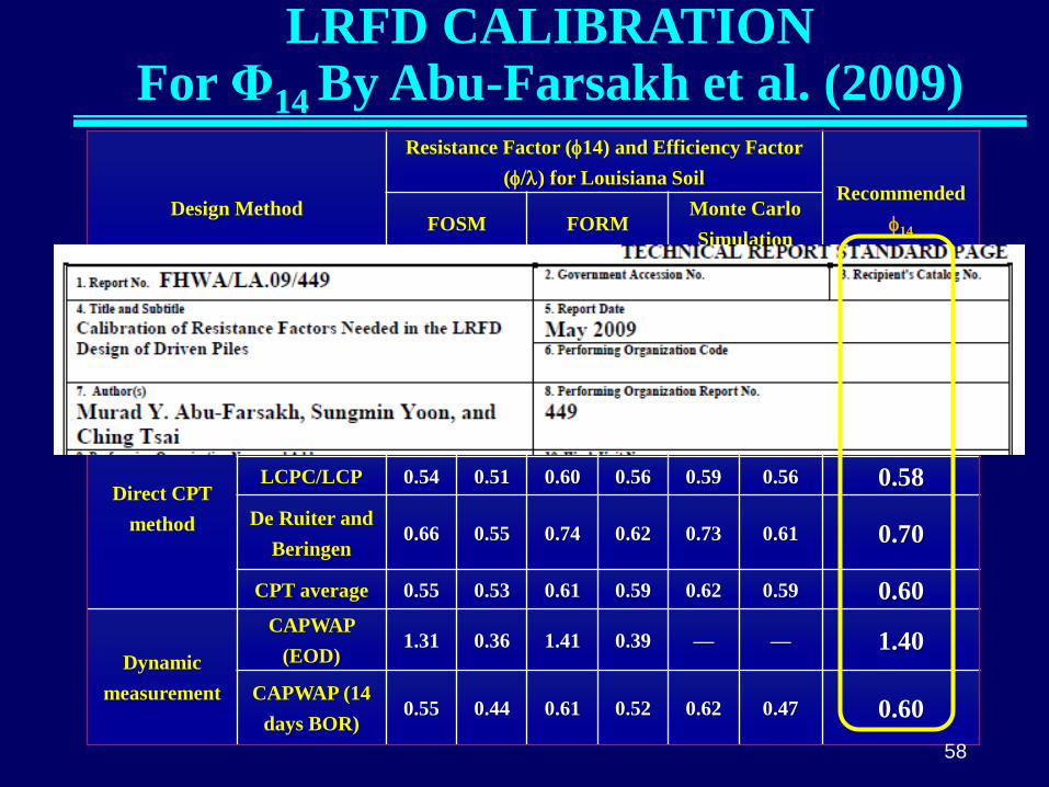
LRFD CALIBRATION For Φ14 By Abu-Farsakh et al. (2009)
Design Method
Resistance Factor (f14) and Efficiency Factor
(f/l) for Louisiana Soil Recommended
f14 FOSM FORM Monte Carlo
Simulation
f14 f14/l f14 f14/l f14 f14/l
Static method
a-Tomlinson
method and
Nordlund
method
0.56 0.58 0.63 0.66 0.63 0.66 0.60
Direct CPT
method
Schmertmann 0.44 0.47 0.48 0.52 0.49 0.53 0.48
LCPC/LCP 0.54 0.51 0.60 0.56 0.59 0.56 0.58
De Ruiter and
Beringen 0.66 0.55 0.74 0.62 0.73 0.61 0.70
CPT average 0.55 0.53 0.61 0.59 0.62 0.59 0.60
Dynamic
measurement
CAPWAP
(EOD) 1.31 0.36 1.41 0.39 — — 1.40
CAPWAP (14
days BOR) 0.55 0.44 0.61 0.52 0.62 0.47 0.60
58
LRFD CALIBRATION
(a) Comparison of (R30 - R14)
for Level-1 (b) Comparison of (R45 - R14)
for Level-1
*Set-up was predicted with the developed models. *Set-up was calculated or LRFD was calibrated for the resistance after 14 days for four different times. 1. 30 days 2. 45 days 3. 60 days 4. 90 days
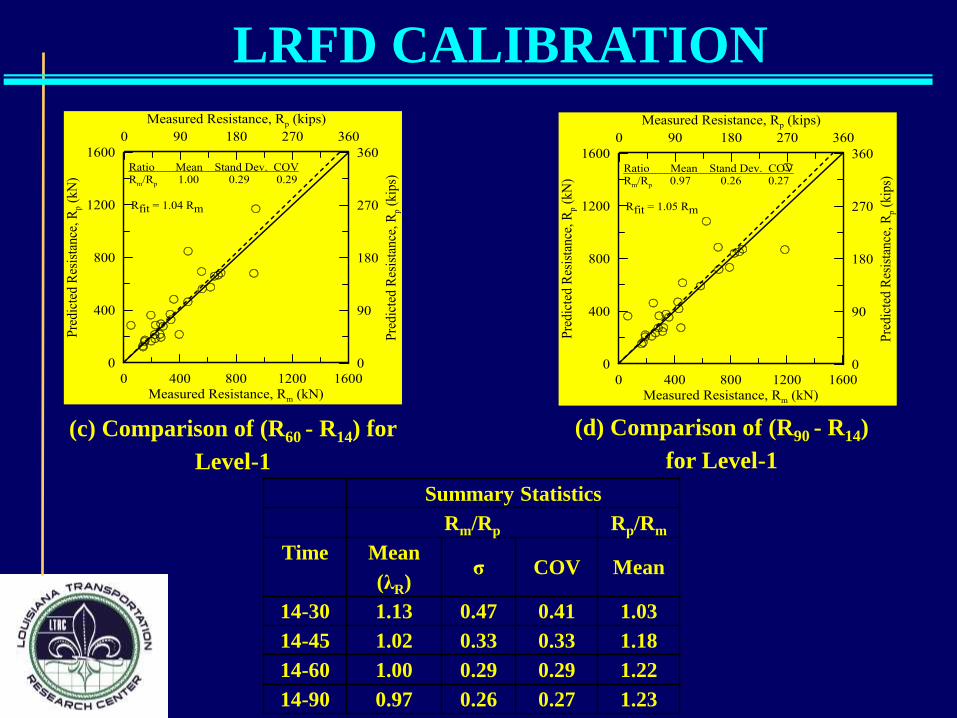
LRFD CALIBRATION
(c) Comparison of (R60 - R14) for
Level-1
(d) Comparison of (R90 - R14)
for Level-1
Summary Statistics
Rm/Rp Rp/Rm
Time Mean
(λR) σ COV Mean
14-30 1.13 0.47 0.41 1.03
14-45 1.02 0.33 0.33 1.18
14-60 1.00 0.29 0.29 1.22
14-90 0.97 0.26 0.27 1.23
Probability Density Function and Histogram
R30 - R14 R45 - R14
R60 - R14 R90 - R14
61
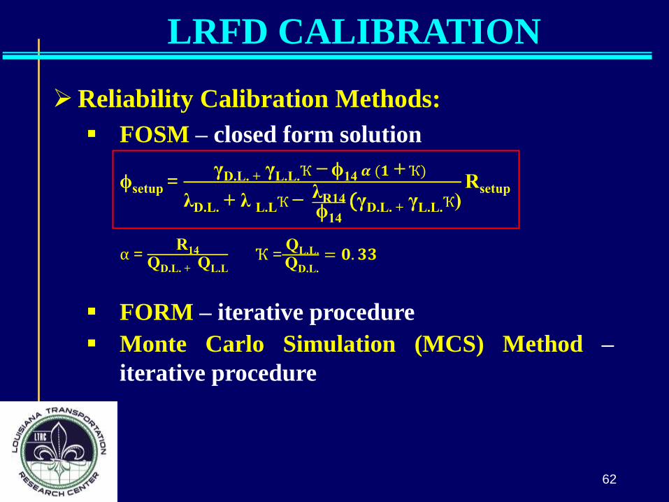
Reliability Calibration Methods:
FOSM – closed form solution
ϕsetup = γD.L. +
γL.L.Ҡ − ϕ14 𝜶 (𝟏 + Ҡ)
λD.L. + λ L.LҠ − λR14ϕ14
(γD.L. + γL.L.Ҡ)
Rsetup
FORM – iterative procedure
Monte Carlo Simulation (MCS) Method –
iterative procedure
62
α = R14
QD.L. + QL.L
Ҡ = QL.L.
QD.L.
= 𝟎. 𝟑𝟑
LRFD CALIBRATION
CALIBRATION RESULTS
R30 - R14 R45 - R14
R60 - R14 R90 - R14
0.30 0.34
0.35 0.35
63
βT = 2.33
Recommended FOSM FORM MC
LTRC @ 14-30 Days 0.28 0.28 0.30 0.30
LTRC @ 14-45 Days 0.32 0.33 0.34 0.34
LTRC @ 14-60 Days 0.34 0.35 0.36 0.35
LTRC @ 14-90 Days 0.34 0.36 0.37 0.35
Kam Ng (2013) 0.36 - -
Yang & Liang (2006) - 0.30 -
Overall Recommended = fsetup = 0.35
setupsetup1414LLDD RRQQ ff
64
CALIBRATION RESULTS
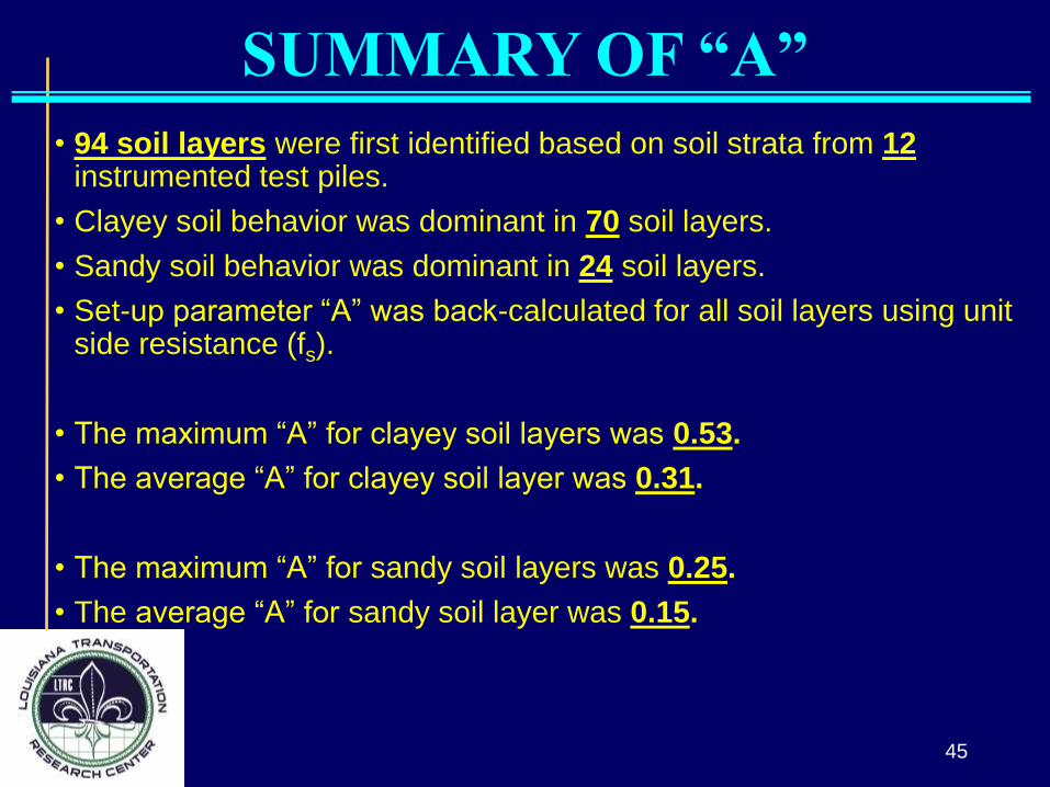
• Set-up study was conducted on 12 instrumented test piles of 5 different sites. Set-up was mainly exhibited by side resistance. The tip resistance was almost constant.
• Set-up was mainly attribute to the consolidation behavior. Amount of set-up and set-up rate increased significantly during consolidation phase. Very small amount of set-up was observed during “aging” period.
• Horizontal effective stress increased significantly during the consolidation period. Once the consolidation period was over, the amount of increase became slower.
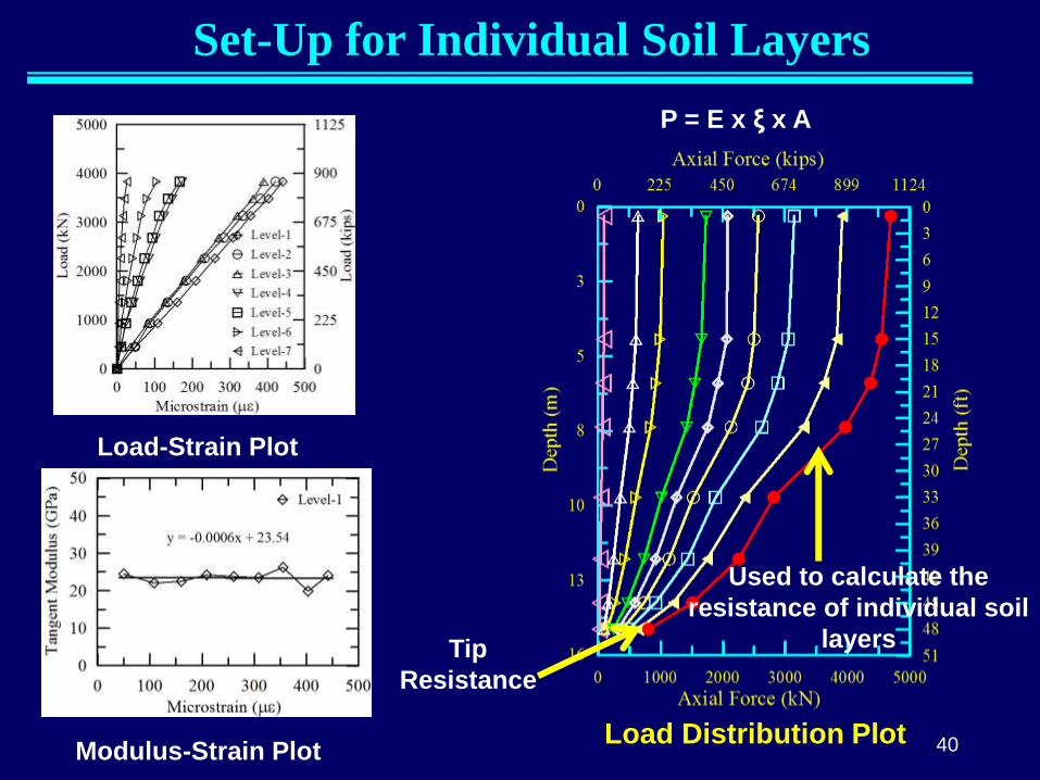
• Set-up for individual soil layers was calculated with the aid of strain gauge.
• The set-up rate “A” for clayey soil layers was 0.31 and for sandy soil layers it was 0.15.
65
CONCLUSIONS
• Three models were developed
• A =0.79∗
PI
100+0.49
Su
1tsf2
.03+2.27
A= f(PI, Su) [Lab Test]
• A =1.12∗
PI
100+0.69
Su
1tsf1
.44 ∗ log
Cv
0.01in2
hour
0.54+3.19
A= f(PI, Su, Cv) [Lab Test]
• A =0.44∗
PI
100S
t+2.20
Su
1tsf1
.94 ∗ log
Cv
0.01in2
hour
1.06+10.65
A= f(PI, Su, Cv, St) [Lab Test]
• Set-up rate can be processed to predict total set-up resistance.
• The recommended set-up factor is 0.35 for LRFD design.
66
CONCLUSIONS
67
• Chen, Q., Haque, Md. N., Abu-Farsakh, M., and Fernandez, B. A. (2014). “Field investigation of pile setup in mixed soil.” Geotechnical Testing Journal, Vol. 37(2), pp. 268-281.
• Haque, Md. N., Abu-Farsakh, M., Chen, Q., and Zhang, Z. (2014). “A case study on instrumenting and testing full scale test piles for evaluating set-up phenomenon.” Journal of the Transportation Research Board No 2462, National Research Council, Washington, D.C., pp. 37-47.
• Haque, Md. N., Abu-Farsakh, M., Zhang, Z. and Okeil, A. (2016). “Estimate pile set-up for individual soil layers and develop a model to estimate the increase in unit side resistance with time based on PCPT data.” Journal of the Transportation Research Board , National Research Council, Washington, D.C. (In Press).
• Haque, Md. N., Chen, Q., Abu-Farsakh, M., and Tsai, C. (2014). “Effects of pile size on set-up behavior of cohesive soils.” In Proceedings of Geo-Congress-2014: Geo-Characterization and Modeling for Sustainability, Technical Papers GSP 234, pp. 1743-1749.
• Haque, Md. N., Abu-Farsakh, M., and Chen, Q. (2015). “Pile set-up for individual soil layers along instrumented test piles in clayey soil.” In Proceedings of the 15th Pan-American Conference on Soil Mechanics and Geotechnical Engineering (From fundamentals to applications in Geotechnics), November 15-18, Argentina, pp. 390-397.