Adaptive Polygonization of Implicit Surfaces Ulises Cervantes-Pimentel Introduction Polygonization of surfaces has many practical applications in computer graphics and geometric modeling. It basically consist in computing a piecewise linear approximation for a smooth surface f described either by implicit, f(x,y,z)=0, or parametric functions. This procedure involves basically two basic operations: Sampling and Structuring. Sampling generates a set of points on the surface and structuring links those points to construct a mesh. In general, algorithms can be classified accord- ing to how they implement these operations. Motivation Polygonization (or tesselation) of a surface f is implemented in Mathematica by the functions ContourPlot3D and ListCon- tourPlot3D. ContourPlot3D is based on a uniform decomposition of the three-dimensional space into cubes of the same size called cells. The function that describes the surface geometry is evaluated at node points of a regular grid. If there is a change on the function sign at node points of a cell's edge, the intersection point P of the edge-surface is computed as a follows for the segment ab : a= f @aD f @aD-f @bD P = P a +a HP b - P a L Uniform decomposition of the ambient space are straightforward to implement, but produce polygonal meshes that are not adapted to the implicit surface. Such solution is only acceptable for shapes with regular features, where the surface curvature is almost constant [LV2]. The fixed sampling rate causes oversampling of areas with low curvature and undersampling of areas with high curvature. In this report we present an algorithm based in an adaptive sampling rate that varies spatially according to local surface complexity. Adaptive polygonization algorithms are more complex than uniform algorithms because they must deal with two relatted problems: i) Ensure optimal sampling. Guarantees a faithful geometric approximation, depends on the adaptation criteria ii) Enforce correct topology. Guarantees the consistency of the mesh and depends on the structuring mechanism local changes to the sampling rate may affect the global mesh topology. For example, different levels of subdivision in two adjacent cells could create a crack along the boundary between them. Presentation.nb 1
Transcript
Adaptive Polygonization of Implicit Surfaces
Ulises Cervantes-Pimentel
à Introduction
Polygonization of surfaces has many practical applications in computer graphics and geometric modeling. It basically consistin computing a piecewise linear approximation for a smooth surface f described either by implicit, f(x,y,z)=0, or parametricfunctions. This procedure involves basically two basic operations: Sampling and Structuring. Sampling generates a set ofpoints on the surface and structuring links those points to construct a mesh. In general, algorithms can be classified according to how they implement these operations.
à Motivation
Polygonization (or tesselation) of a surface f is implemented in Mathematica by the functions ContourPlot3D and ListContourPlot3D. ContourPlot3D is based on a uniform decomposition of the three-dimensional space into cubes of the same sizecalled cells. The function that describes the surface geometry is evaluated at node points of a regular grid. If there is achange on the function sign at node points of a cell's edge, the intersection point P of the edge-surface is computed as afollows for the segment ab
èèè:
a = f@aDÄÄÄÄÄÄÄÄÄÄÄÄÄÄÄÄÄf@aD-f@bDP = Pa + a HPb - PaL
Uniform decomposition of the ambient space are straightforward to implement, but produce polygonal meshes that are notadapted to the implicit surface. Such solution is only acceptable for shapes with regular features, where the surface curvatureis almost constant [LV2]. The fixed sampling rate causes oversampling of areas with low curvature and undersampling ofareas with high curvature.
In this report we present an algorithm based in an adaptive sampling rate that varies spatially according to local surfacecomplexity. Adaptive polygonization algorithms are more complex than uniform algorithms because they must deal with tworelatted problems:
i) Ensure optimal sampling. Guarantees a faithful geometric approximation, depends on the adaptation criteria ii) Enforce correct topology. Guarantees the consistency of the mesh and depends on the structuring mechanism
local changes to the sampling rate may affect the global mesh topology. For example, different levels of subdivision in twoadjacent cells could create a crack along the boundary between them.
Presentation.nb 1
Following are some examples comparing the current implementation of ContourPlot3D and an adaptive polygonization.
The present work is based in the paper "A Unified Approach for Hierarchical Adaptive Tesselation of Surfaces", [LV1].
This algorithm combines hierachical curve sampling with simplicial subdivision. It is composed of three independentoperations:
ü Base mesh generation:
A very coarse sampling grid suffices for most implicit shapes of interest. Knowledge about the surface should be used todetermine the appropiate uniform sampling rate. For a compact surface of genus 0, the shape should be smaller then thediameter of the largest sphere inscribed in the shape
The base mesh generation decomposes the bounding box of the implicit shape using a simplicial cell complex. It then identifies the set of cells that are intersected by the implicit surface and for each of these cells it generates an element of thepolygonal mesh approximating the surface. As in [LV2], we use a simplicial decomposition know as Coxeter-Freudenthalsubdivision, that is defined as follows: For a cube in R3 with vertices p0 , p1,..., p7, it takes the diagonal p0 p7 and projects itonto each face of the cube. This gives a triangulation of the faces of the cube. The 3D simplicial cells are constructed byadding to each triangle in a face, the vertex of the diagonal p0 p7 that does not belong to it. We obtain:
Presentation.nb 4
CFdecomp = 881, 5, 6, 8<,81, 5, 7, 8<,81, 2, 6, 8<,81, 2, 4, 8<,81, 3, 7, 8<,81, 3, 4, 8<<;When a potential hit occurs, the Coxeter-Freudenthal decomposition of the cube is generated and each of its simplices areprocessed.
Note that the choice of the diagonal p0 p7 is arbitrary. We can of course chose any of the other three diagonal as well.During the initial subdivision we can choose to test any of these decompositions and select the one that generates the"best" triangulation. The option CFDecomposition->L, where L is a sublist of {1,2,3,4}, has precisely this effect.
cubepermutations = 881, 2, 3, 4, 5, 6, 7, 8<,85, 6, 7, 8, 1, 2, 3, 4<,83, 4, 1, 2, 7, 8, 5, 6<,82, 1, 4, 3, 6, 5, 8, 7<<;As an example of the effect of this option, consider the following surface:
sigmoid@d_ ê; d £ 1D := 1 - H4 d^6 - 17 d^4 + 22 d^2L ê9sigmoid@d_ ê; d > 1D := 0.Saucer@x_, y_, z_D := z - sigmoid@Sqrt@x^2 + y^2DD ê 3
Based on the sign of f, possible intersections of the simplex with the surface are tested. Note that, when the parent cube isintersected by the surfaces only some cells of the simplicial decomposition will be crossed by it. The implicit surface mayintersect the edges of a simplex in either three or four points. Orientation of the triangles is asserted by requiring that thenormal points in the oposite direction to a negative vertex.
Intersection of an edge with the surface can be computed in two different ways. It can be estimated as a proportional valuesas in ContourPlot3D or by bisection. The number of iteration in the last case is controled with the option MaxBisectionIter.The way the intersection is estimated is controled with the option IntersectionStyle->0 for the bisection case and IntersectionStyle->1 for the proportional case.
X = DimL = `Log nxp, M = `Log nyp, N = `Log nzpIndex = -8L, M, N, X, X, X<CornerVertex Hl, m, nL8l, m, n, 0, 0, 0<MiddlePoint Hl, m, nL, Hp, qL
r = p^q, s = p & qp' = p^s, q' = q^s8l + s2, m + s1, n + s0, r, 0, 0<
Edges Hl, m, nL, Hp, qL, p < q8l + s2, m + s1, n + s0, 0, p', q'<
ü Edge sampling
The edge representation is constructed using a hierarchical sampling. This scheme generates a multiresolution, adapted,piecewise-linear approximation of the corresponding curve on the surface. This procedure subdivides the edge PQ at itsmidpoint M, and finds a new sample, the split point T on the surface. It also computes the difference between these twopoints, the vector D=T-M. Recursion terminates when the maximum sampling density, set by MaxAdaptiveRecursion isreached or an edge is found to be Flat.
We need to find a point on the implicit surface f -1H0L that is closest to the edge midpoint M. The problem amounts tocomputing the point T such that f(T)=0 and, at the same time minimizes the distance þT-Mþ. This can be solved using anumerical technique such as gradient descent. However, we employ a physically-based method [LV1]. In its simplest version,the method is:
d=SteepestDescentStepwhile Èf(x)È>Tolerance
y¬f(x)x¬x-d sign f(y) Ñf(x)if sign(y)!= sign(f(x)) then d¬d/2
The criteria to classify an edge as FLAT or NOTFLAT is controlled by the option AdaptiveStyle. It can take the values:
0: The surface curvature along an edge is measured by the angle a between the surface normals at the edge endpoints.If theangle is greater than FlatnessAngle, the edge is classified as not flat.
Presentation.nb 10
8$FlatnessAngle, $AdaptiveStyle<860, 0<Saddle@x_, y_, z_D := z - Hx y L^3Show@GraphicsArray@
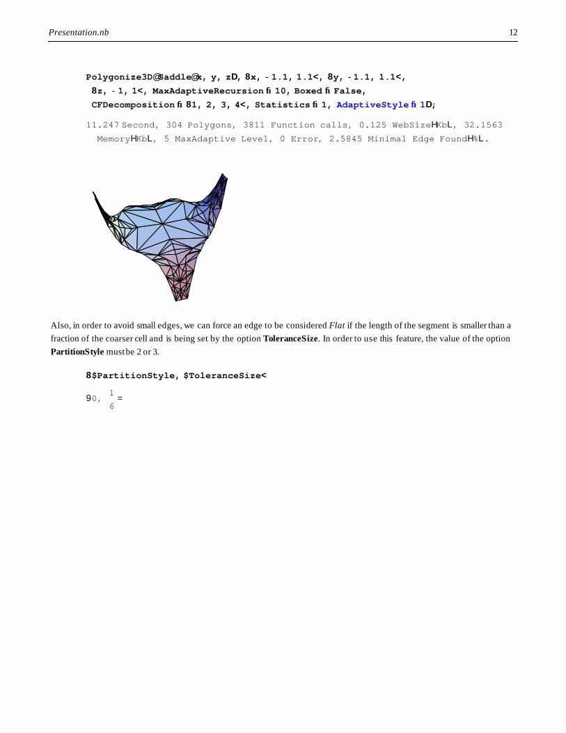
Also, in order to avoid small edges, we can force an edge to be considered Flat if the length of the segment is smaller than afraction of the coarser cell and is being set by the option ToleranceSize. In order to use this feature, the value of the optionPartitionStyle must be 2 or 3.
It is also possible to specify a trimming function. Once an edge is classified as Flat, if the option Trimming defines a function, the adaptive edge generation subrutine will generate a vertex by finding the intersection of the segment with thespecified function.
The cell structuring operation performs a simplicial decomposition. It recursively subdivides a triangular cell into triangularsubcells, using information from its edges. For this purpose, new internal edges are created and adaptively sampled.
The figure below shows the different cases:
Presentation.nb 14
note that for the cases where two or three edges are not flat, we have different options in subdividing the cell. The Qualitycriteria is specified with QualityForm. The different options are generated and the best triangulation is selected.
Q1 = lminÄÄÄÄÄÄÄÄÄÄÄÄR
Q2 =r
ÄÄÄÄÄÄÄÄÄÄÄÄlmax
Q3 =rÄÄÄÄÄR
Q4 = lminÄÄÄÄÄÄÄÄÄÄÄÄlmax
Q5 =A
ÄÄÄÄÄÄÄÄÄÄÄÄÄÄl2max
Q6 = Min@Cos@aiDDQ7 = Max@Cos@aiDD
If PartitionStyle is equal to 1 or 3, the cells structuring will test all possible subdivisions. This can make the method runmuch slower than needed. Normally it is only necessary considering the first case of the three nonflat edges case.
I) [Initialization]Start with a coarse decomposition of the surfacea) Generate the base meshb) Sample the edges of all cells in the base mesh
II) [Refinement]For each cell, test the corresponding surface patch for flatnessIf the patch is not flat, then recursively subdivide the cella) Structure new cells by constructing internal edgesb) Sample all internal edges
The procedures implementing structuring and sampling operations comunicate through a well-defined inyterface: the edgeand cell data structures
Data structures for vertex, facets and adaptive edges have being implemented in three different ways:
i) Mathematica Lists. Append[] and Position[]ii) Caching values. See examples aboveiii) ExpertBags.
The following are graphs of running times, function calls and memory requirements:
V1: No data structure. Repetive function evaluation.V1c: No data structure. Cachinf function values f[x_]:=f[x]=...V2: Data structure implemented using i)V2c: Data structure implemented using ii)V3: Data structure implemented using iii)
Polygonize3D is the tetrahedral analog of CountourPlot3D which also includes adaptive refinement.
Polygonize3D will plot surfaces showing particular values of f as a function of x, y and z. Polygonize3D works by dividing thethree-dimensional space into cubes and deciding if the surface intersect each cube. If the surface does intersect a cube,Polygonize3D will subdivide this cube further, and so on.
Presentation.nb 26
ContourPlot3D@ f, 8x, xmin, xmax< , 8 y, ymin, ymax< , 8z, zmin, zmax< D generate a threedimensional contour plot f
Plot3DWeb@level, quality, gap, normalsD generates a three - dimensionalplot of
This loads the package
<< Polygonize`Polygonize3Dtrm`
<< "D:\Wolfram\Polygonize\Polygonize3Dtrm.m"
This produces a three-dimentional plot of a zero values of the function.
Contours 80.< the list of values for the contours to be plottedContourStyle 8< the list of styles for the contours to be plottedMaxRecursion 1 the number of levels of recursion used in each cube
PlotPoints 83,5< the number of evaluation points to use in each direction
MultiGrid $MultiGrid = 0 Data stored :0 : Just higherlevel, initialreset data
1 : All levels , initialreset data2 : All levels , no initialreset data
Statistics $Statistics = 0 Verbosereport
Trimming $Trimming = 0 Trimming function
Options for Polygonize3D
Each value specified in Contours generates a different surface. ContourStyle colors each surface. To use this option,you must set Lighting -> False. MaxAdaptiveRecursion sets the number of times you subdivide each initial
triangle. However, if the surface does not intersect the cube, the cube is not subdivided into tetrahedrals and no initialtriangles are generated. If MaxAdaptiveRecursion is greater than 0, adaptive recursion takes place. Polygonize3D and
Plot3DWeb return a Graphics3D object. This means the functions will accept any option that can be specified for a
Graphics3D object.
Here is another plot showing a contour value of -0.2 and 0.0.
Contours 80.< level plotted, 0->All levelsContourStyle 8< Cuttoff criteria foraspect ratioMaxRecursion 1 Plotting gapPlotPoints 83,5< Include triangle normals in plotting
Parameters for Plot3DWeb
à Polygonize`DataHandlingv3`
Presentation.nb 29
à Bibliography
[LV1] Luiz Velho & Luiz Henrique de Figueiredo, "A Unified Approach for Hierarchical Adaptive Tesellation of Surfaces" ,ACM Transactions on Graphics, Vol. 18, No. 4, October 1999, pp 329-360.
[LV2] Luis Velho, "Simple and efficient polygonization of implicit surfaces" , J. Graph. Tools 1,2,5-24, 1996.
[JB1] Jules Bloomenthal, "Polygonization of Implicit Surfaces" , Xerox Corporation, CSL-87-2 May 1987
[JB2] Jules Bloomenthal & K. Ferguson, "Polygonization of Non-Manifold Surfaces" , Research Rep. 94-541-10, Dept. ofComputer Science, The University of Calgary, June 1994.