Implementation of the vehicle recognition systems using wirelessmagnetic sensors

SERCAN VANCIN and EBUBEKIR ERDEM*

Department of Computer Engineering, Firat University, 23100 Elazig, Turkey

e-mail: svancin@firat.edu.tr; aberdem@firat.edu.tr

MS received 23 May 2016; revised 26 October 2016; accepted 23 November 2016

Abstract. Wireless network sensors and their use in traffic monitoring, traffic density determination or vehicle

speed detection and classification have recently been the focus of interest for researchers. This article describes

how a new sensor circuit was designed to deliver instantaneous, real-time and novel solutions as a vehicle

detection system, which is more powerful than the nodes used in other studies, and gives results with smaller

error margins due to its serial communication qualification. With the proposed logic algorithm, it was possible to

categorise the instantaneous traffic status of a road in four levels: no traffic, mild traffic, heavy traffic and very

heavy traffic. Additionally, with the nodes placed at the beginning and the end of the road, the number of

vehicles per hour for a day was determined and traffic was analysed. Then, vehicles passing by were classified

with a proposed classification algorithm and magnetic signature length (MSL) parameter as cars, minibuses,

buses and trucks, and an accuracy rate of 95% was obtained. As the last application, the direction of motion of

the vehicle on the x-axis as well as left-to-right or right-to-left directions was determined, and the result was 94%

accurate. The simplicity of the proposed algorithms, the absence of any complex mathematical calculations, the

low cost of the sensor node and circuit and the low power consumption of the communication system

demonstrate the superiority of this system in comparison with other studies.

Keywords. Wireless sensor networks; magnetic sensor; traffic congestion; vehicle detection; magnetic

signature length.

1. Introduction

Recently, several people face transportation problems and

traffic jams. In order to monitor traffic, collect information

on traffic status and transmit this information to drivers,

intelligent transportation systems (ITS) were designed [1].

These systems operate by counting the number of vehicles

on the road and determining the speed of the vehicles or by

acquiring images of the vehicles through video cameras. As

a result, traffic jams can be reduced by traffic information

analysis or traffic forecast [2].

Many studies report the development of vehicle identi-

fication system by wireless sensor networks. Traffic con-

ditions of the roads have been examined using anisotropic

magnetic sensors (AMRs) and microphone sensors [3]. In

addition to these, acoustic sensors [4], ultrasonic sensors [5]

and video camera analysis systems or aerial images [6]

have been used as a part of vehicle identification with

wireless sensor network technology. In another study,

magnetometer sensors were used [7]; magnetic fields

detected above a threshold were measured in time as sig-

nals identifying the vehicles and thus compass applications

were developed. Yet another study designed a real-time

traffic control system using wireless sensor networks [8]. In

another study, a traffic monitoring system integrated with

mobile data imaging and, as a result, management was

suggested [9]. Vehicle identification was made using

wireless sensor networks with multiple sensors and light,

middleweight and heavy vehicles were classified [10]. To

classify the vehicles on the road, an optimally divided

sample-based classification and regression tree algorithm

(CART) was suggested in a study by Haijian et al [11]. A

neural networks-based vehicle motion-mode identification

method was proposed [12]. In a study conducted by Varaiya

and his students [13], magnetic data in z-axis were deter-

mined as the minimum and maximum and threshold values

were detected for traffic surveillance using wireless mag-

netic sensors.

In this study, sensor nodes that can operate in a multi-

purpose way were designed and the sensor circuits were

built by implementing magnetic sensors (HMC5983L) on

those nodes. The sensor nodes were designed to be cheaper

than the other nodes on the market, such as TelosB or

MicaZ. With the help of those sensor circuits, three dif-

ferent applications were developed. The first of these

applications was the real-time detection of the four-level*For correspondence

841

Sadhana Vol. 42, No. 6, June 2017, pp. 841–854 � Indian Academy of Sciences

DOI 10.1007/s12046-017-0638-4

instantaneous traffic information from a single-lane road

using multiple sensor nodes. These levels were no traffic,

mild traffic, heavy traffic and very heavy traffic. The rel-

evant traffic density was obtained with the suggested logic

value finding algorithm. Among the greatest advantages of

this method when compared to others [3, 11] were the use

of multiple sensor nodes, the minimisation of analog data

measurement errors through serial communication of the

nodes, low-cost system components and high perfor-

mance. Additionally, with the help of a node that is placed

at the end of the road (Node 3), a 24-h condition of traffic

was observed hourly as a part of this application. In the

second application, the vehicles passing by were classified

as cars, minibuses, buses and trucks. In previous studies,

pattern recognition using inductive loop detectors [14] and

valley-and-hill pattern models using magnetic sensors

[15, 16] was suggested for vehicle classification. In this

study, however, a magnetic signature length (MSL) con-

cept was defined and suggested as a novel solution to the

classification problem. MSL presented excellent solutions

to the vehicle classification problem with the developed

algorithm (classification algorithm) and made it possible

to obtain more accurate results than the ones in the study

by Haijian et al [11]. In the Haijian et al [11] study,

vehicles were only classified as automobiles or buses; but

in the present study, classification was made in four cat-

egories and with a short-time decision mechanism.

Finally, direction of motion in the x-axis was determined

for vehicles with the aforementioned sensor circuits. The

use of only two sensor nodes and the high performance of

the invented direction determination algorithm show that

this study is superior to the previous works. The per-

centage accuracy was examined in a setting where 50

vehicles made pass by the road, from left to right and from

right to left. It was seen that this study gave more accurate

results than the previous study [10]. On the other hand,

construction of the system with low-cost hardware devices

was possible due to the structure of the designed wireless

sensor network. This wireless sensor network has its

superiority in the programming simplicity of the magne-

tometer and the sensor nodes used and in the transmission

of the necessary information to the coordinator node in a

star topology. Sensor nodes and magnetometer were

connected in series communication to avoid complicated

computations and obtain more accurate information. In

order to avoid traffic jams, the acquired information—

such as the traffic condition, vehicle type or direction of

motion—could be sent instantaneously over the Internet to

drivers who wished to enter the road under study.

The remainder of this paper is organised as follows.

Section 2 summarises the topic of wireless sensor net-

works. Section 3 details the topic of magnetic sensors and

the realisation of the system with an explanation of the

thought scenario. Section 4 presents the experimental

applications and system analysis are presented in three

subsections. Lastly, section 5 discusses the results of this

study and gives suggestions.

2. Wireless sensor networks

Wireless sensor networks are scattered network structures

in which many sensors or sensor nodes are in wireless

communication. Wireless communication occurs between a

receiver and a transmitter without cable connections via

light or electromagnetic waves. Sensor networks built with

small devices are cheap and have the ability of self-or-

ganisation, which makes the sensor intercommunications

easier. Sensors, also called detectors and probes, are the

sensing elements in electronic applications. The main

components of a sensor node are the microcontroller,

receiver–transmitter, power supply, memory and one or

more sensor components. Various node types are on the

market, such as TelosA, TelosB, Mica2, MicaZ, eMote,

IMote2 and Sensenode, all of which can be used in wireless

sensor networks [16–18].

A sensor has the ability to detect many physical quan-

tities such as length, amount, area, mass flow, heat

transfer, force, temperature, voltage, current, resistance,

oxidation/reduction, flux density, condensation, content,

magnetic moment and magnetic field. Those different

sensors can be used in many different fields according to

their uses [19, 20]. For example, heat transfer or temper-

ature measurements can be used to work against forest

fires, whereas measurements with moisture, temperature

or pressure sensors can be used in weather forecasting and

so forth. To measure the magnetic field of the Earth, to

identify a certain material or to determine the metallic

properties of objects, anisotropic magnetoresistive sensors

(AMRs) are used [21–23]. Because metals such as iron,

nickel or cobalt affect the background magnetic field,

many objects containing metals can be detected by these

sensors. Because vehicles contain various metal parts as

well, they can be detected using magnetic sensors. Simi-

larly, traffic information on a road can also be obtained

[24–26].

3. Magnetic sensors and experimental systemsetup

Magnetic sensors have been used for a long time. Although

the early works were on basic direction finding and navi-

gation, nowadays these applications have expanded. Mag-

netic sensors that can make more precise and more accurate

measurements are now designed to work conveniently with

integrated circuits. They have become more advantageous

842 Sercan Vancin and Ebubekir Erdem

in terms of both size and cost; accordingly, anisotropic

magnetoresistive sensors (AMRs) have been developed that

can optimally detect the magnetic field of the Earth [7, 27].

Apart from containing 16 pins in its inner structure, an

HMC9583L sensor (figure 1) has four usable pins on the

outside. These are SDA/SPI_SDI, SCL/SPI_SCK, GND

and VDD (2.16 v–3.6 v) pins (figure 2(b)). The GND pin

is for grounding and the VDD pin is to establish a power

connection. To operate the sensor at 3.3 v through VDD, a

power board circuit and a power supply (AA battery) were

used. The main reason for using this sensor in this study is

the possibility of serial communication when connected to

the sensor node via pins with an I2C port. Thus, magnetic

information is recorded in the data registers (X, Y and Z)

in a binary mode with the processor of the sensor node

after every clock period obtained via the SCL (Serial

Clock) pin. The measurement method of the magnetic

sensor via configuration registers A and B was adjusted to

normal measurement mode because the measurement is

done on the rising side of every clock period and data in

the registers are updating. The information in these

recorders can be used if necessary. This information

gathered in the registers is transmitted to the sensor node

via the SDA (Serial Data) pin at a serially determined

frequency (128 Hz). On the other hand, for the clock

frequency, CRA4, CRA3 and CRA2 bits in register A

were made logic ‘‘1,’’ ‘‘0’’ and ‘‘0,’’ respectively. In this

way, both more precise data were obtained. The magnetic

field for each of the three axes was obtained by the con-

version of the 2-byte magnetic value at each data register,

X, Y and Z, to its value in modulo 10. Finally, the

resultant value (C) was calculated with the help of the

following equation.

C ¼ffiffiffiffiffiffiffiffiffiffiffiffiffiffiffiffiffiffiffiffiffiffiffiffiffiffiffi

X2 þ Y2 þ Z2p

ð1Þ

The C value increases when a vehicle gets close to the

nodes because the vehicles contain copious amounts of

iron, nickel and cobalt (ferrous mass) and they alter the

background ferromagnetic field. The magnetic field of the

Earth is approximately 500 mGauss by default and the

measured value increases when a vehicle passes a magnetic

sensor within 0.5–1 m. If the C value is divided by 256, the

magnetic field is found in units of gauss. For example, if the

C value is 280, then the magnetic field at that point is 1.09

gauss. A magnetic change in each direction causes a change

in C. During vehicle detection with an HMC5983L mag-

netometer, the C value is grounded. If a vehicle passes by a

magnetic sensor placed on the side or in the middle of the

road, the measured C value exceeds the threshold

ðCthresholdÞ and it is understood that a vehicle is on the road.

Hence, the vehicle is detected.

The new sensor circuit used throughout the study for

vehicle detection systems alongside the power board and

the battery can be seen in figure 2 and the circuit block

diagram in figure 3. The sensor node, which operates under

the Zigbee IEEE 802.15.4 standard in the 2.4 GHz ISM

band and maintains small size data intermission, is a low-

cost device and a very low-power-consuming wireless

sensor node. The designed wireless sensor node is a PA/

LNA-based Zigbee SoC (system-on-chip) integrated

CC2530 and CC2591 manufactured by Texas Instruments.

It was empowered with an MSP430, Ultra-Low-Power

microcontroller unit (MCU). The difference between this

node and the others such as TelosB or micaZ is that its

hardware components can be optionally assembled. On this

sensor node, SHT11 temperature and moisture sensor and

Electronically Erasable Programmable Read Only Memory

(EEPROM) are present alongside the many connectors that

can be helpful in studies. Additionally, it contains a UART1

connector, to which a Sim900 node can be connected in

Figure 1. HMC9583L magnetic sensor integrated circuit.

Figure 2. A sensor circuit designed for vehicle detection.

Implementation of the vehicle recognition systems 843

order to transfer the collected data to the Internet and a

UART2 connector to monitor the serial port output. As seen

in figure 2, HMC5983L (magnetic sensor), which directly

connects to the I2C port of the sensor node, can use the

sensor as a compass along three axes. During the design of

the sensor circuit, the 3.3-v output of the power board was

connected to the VCC pin of the sensor circuit, as seen in

figure 3. The angle with the magnetic poles of the Earth can

be found using a 12-Bit Analog Digital Converter (ADC)

with 1�–2� sensitivity.

Additionally, the sensor on the axes can communicate

with the sensor nodes via the I2C protocol when a metal

object gets close to the compass sensors. During the pro-

gramming of the sensor, all the values on the sensor axes

were read and the resultant value (C) was calculated using

Eq. (1). If the sensor is used to just observe the effects of

other objects on the magnetometer and not as a compass,

then the resultant value will be enough. In this case, the

resultant value, which is different at every place, changes

when a metal object passes by. In this way, metal objects

around the sensor can be identified.

4. Experimental applications

After the design of the multi-purpose sensor node and the

circuit, three applications were performed as an experi-

mental work and results were analysed using Matlab soft-

ware. First of all, the four-level instantaneous traffic jam

information of a single-lane road was obtained via vehicle

detection by the magnetic sensor mounted on the sensor

nodes. Then the vehicles passing by are classified in one of

four categories: cars, minibuses, buses and trucks. Last, the

direction of a passing vehicle was determined as being from

left to right or from right to left.

4.1 Determination of the traffic congestion

In this part of the study, vehicle detection was due to the

metal found on and in the vehicles. In this application, the

wireless sensor network was constructed in order to detect

the traffic condition on a 100-m road with three sensor

nodes placed as in figure 4. Each sensor node was pro-

grammed using C language with the Code Composer

Studio open-source software. The three nodes used in the

study were programmed as the end device (ED), whereas

the other communal node was programmed as the coor-

dinator. In fact, the coordinator node is not different from

the other nodes; it just obtains the magnetic data simul-

taneously from the other three sensors due to the star

topology of the design. Network setup starts when the

coordinator node is turned on by means of the power

board. There must be a coordinator node in every Zigbee

network. During the programming of this node, PAN ID

was assigned. Usually the assigned ID is 0x0000. This

process reflects the identity of every network. When the

Node 1, Node 2 and Node 3 sensors, which are all EDs,

are turned on with the power board, the coordinator sends

out a request to join the network for every predefined

tm measurement timeð Þ.The coordinator node was programmed according to a

linear algorithm; in other words, the coordinator sends a

simultaneous request to each ED node and waits for an

answer for every tm period, which can be interpreted by

the blinking yellow light on the nodes. When the EDs

join the network and send data to the coordinator, the

yellow light glows. The coordinator node assigns a

16-bit Short Address to the ED that joins the network.

This is the network address that distinguishes every

node. ED nodes transmit the magnetic data collected

from their surroundings to the coordinator node via RF

(Radio Frequency) waves under the Zigbee communi-

cation standard; thus, the utilised network topology is a

star topology. Because the coordinator node is con-

nected to the computer with the programming interface

via USB, the data acquired can be examined with the

Tera Term serial port software. These data were

imported to the Matlab workspace environment with the

serial communication feature found in Matlab. Using

the necessary parameters, the results were plotted in a

graph.

4.1a Proposed algorithm for detection of the traffic con-

gestion: In this study, an algorithm was proposed to

determine the traffic congestion via vehicle detection. For

this, three nodes were placed alongside the road at certain

intervals and the results obtained were analysed. The

resultant magnetic field value was calculated from the

magnetic field values Mx; My and Mz obtained by Node 1,

Node 2 and Node 3 with HMC5983L using Eq. (1). In

previous studies [7, 15], only Mx or Mz values were taken

into consideration to detect vehicles. But the background

magnetic field is a vector quantity in three dimensions, so in

this study the resultant field from three axes is used. The

algorithm to determine traffic conditions is defined in

Algorithm 1.

Figure 3. Block diagram of the sensor circuit.

844 Sercan Vancin and Ebubekir Erdem

Algorithm: Proposed Logical Algorithm()

Input: : Maximum Vehicle Speed

: Minimum Vehicle Speedℎ ℎ : Threshold for Magnetic Resultant: Distance between two sensor nodes

X: Number of significant 8 bits in magnetic data register

Output: 1… , n ≤3: Vehicle detection flags for sensor

nodes (Node 1, Node 2 and Node 3), respectively.Variables:

: Maximum C value( ): C reading for a determined value

: Balanced time according to ( )

Node( ) :Sensor nodes:Minimum time for vehicle passing through the two sensors: Maximum time for vehicle passing through the two sensors

: Sensor delaying time: Time for each sensor measurement

1… , n ≤3: C readings for sensor nodes (Node 1, Node 2 and Node 3), respectively.Algorithm:Main:Initialize the sensor nodes,

ℎ ℎ ← 255,

↓ 50 meters

X← 8,

Compute , ,

← ( + )

2,

≥ ,

while each ( and Node( ) , ≤3 ) and ≤30 minutesif ( )> ℎ ℎ

if ( ) ≤ ( ) ≤then

( )↓ ( )+( + 1) ↓ ( + 1)+

else do then

( ) ↓ ( )-( + 1) ↓ ( + 1)-

end↓ ( )

( ) ← 1,

( ) ← 0else then

90

endend

In the main part of Algorithm 1, sensor nodes are acti-

vated. In the study, Cthreshold was determined as 252 at first.

But this value may change at different places, because the

background magnetic field may be different for different

places on Earth. Therefore, after many experimental

applications, as seen in Algorithm 1, the Cthreshold value was

updated to 255. It was assumed that for the values below

255 ‘‘there was no vehicle’’ and for the values above 255

‘‘there was a vehicle,’’ because there was the concern that

the magnetic sensor may be affected by the other metal

objects around. The important aspect here was that the

information on existence of a vehicle was transmitted only

for the C values above the threshold value. This means that

the information acquired at the intervals when there was no

vehicle detection was ignored. As seen in Algorithm 1,

whenever a vehicle was detected by a node, detection flag

(Nf ið Þ) was fixed as ‘‘1’’ for td delayingtimeð Þ seconds.

After this time, (Nf ið Þ) was assigned to ‘‘0’’. Because a

vehicle can only travel between the minimum and maxi-

mum speeds Vmin and Vmax (km/h) it can travel the dis-

tance between any two nodes in a time interval between

tmin and tmax (s). Therefore, td was taken to be between

tmin and tmax. The C tð Þ value, which was defined to

determine the adaptive td time, was considered to be low

for the vehicles travelling at high speeds and high for the

vehicles travelling at low speeds, because fast vehicles will

have a shorter interaction time with the ground and,

therefore, spends a shorter time in the coverage zone of the

magnetic sensor with respect to slow vehicles. Therefore,

the magnetic change induced by the vehicle that spends less

time in the coverage zone will be smaller and its C value

will be less than the one induced by a slow-travelling

vehicle. According to Algorithm 1, if Sc ið Þ was bigger than

a certain C tð Þ value, the equaliser timeðtoffsetÞ was added to

td time; otherwise, toffset time was subtracted from td time.

Additionally, with td i þ 1ð Þ; the time for the next node to

wait for was also adjusted. The measurement time of the

sensor nodes, tm, must be bigger than or equal to td;because it gives more accurate results to take another

measurement after a longer time than the waiting period. In

addition, it was understood from the experiments that the C

value was also affected by the size of the vehicle. This was

interpreted as larger vehicles, like a truck or a bus, contain a

larger amount of metal. If the C value exceeded the

threshold value Cthresholdð Þ; the case of the vehicle being

near the sensor was recorded as logic 1. As it is understood,

when any of the sensors detects a vehicle, this event is

assigned as ‘‘1’’ by the program. When there is no vehicle

detection, the value is ‘‘0.’’ The algorithm to determine the

traffic congestion relies on the interpretation of the mag-

netic information coming from the sensors as ‘‘1’’ or ‘‘0.’’

Traffic density was evaluated in four categories. For

example, if all the values coming from the sensors were

‘‘1,’’ then there is a ‘‘very heavy traffic’’ condition, and if

all the values were ‘‘0,’’ then there is no traffic. Table 1

identifies all the possible traffic conditions. As seen in

table 1, if Node 1 gave ‘‘0,’’ Node 2 gave ‘‘1’’ and Node 3

gave ‘‘1,’’ the traffic was considered heavy. On the other

hand, since Node 1 was placed at the beginning of the road

Implementation of the vehicle recognition systems 845

and Node 3 at the end, a vehicle goes first by Node 1, then

Node 2 and then reaches Node 3. Considering that the road

is single lane and the vehicles have a Vmax ¼ 60 km/h, the

minimum travel time between the two nodes, 50 m apart, is

tmin = 3 s. Additionally, for a minimum speed,

Vmin ¼ 40 km/h, maximum travel time is tmax ¼ 4:5 s.

Therefore, according to Algorithm 1, td ¼ 3:75 s. On the

other hand, tm was determined to be 4 s, since it must be

bigger than td.

Figure 5 gives two images of the vehicle passing by the

sensor. During the experiments, for the cases where C tð Þ had

the limiting value 260, toffset value was determined as

0.25 s. Hence, if C tð Þ � 260, then toffset value was added to

td; otherwise, it was subtracted. For this application, the

traffic condition was monitored for a 30-min period; the

data to be examined was sent to Tera Term software via a

serial port and then imported to Matlab software. But with a

sampling logic, only the data between 14:20:25 and

14:20:56 are evaluated. Hence, the instantaneous traffic

information was recorded for 31 s. The data were plotted

using Matlab software, where the time 14:20:25 was taken

as the 0th and the time 14:20:56 as the 31st second. Fig-

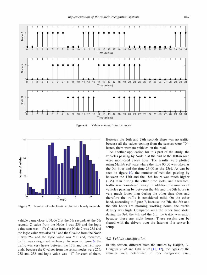
ure 6 shows the information that came from the nodes for

every second. As can be seen, for every second data coming

from the nodes is ‘‘0’’ or ‘‘1.’’ For example, for the 0th and

the 1st seconds, C value from Node 1, Node 2 and Node 3

was 252 (252\Cthreshold) and it was determined that there

was no traffic due to logic value being ‘‘0.’’ But at the 2nd

second, a vehicle entered the road and the value measured

by Node 1 became 258 and a logic ‘‘1’’ was sent. Then this

Table 1. Condition of the traffic according to the sensor data.

Node 1 Node 2 Node 3 State of traffic

0 0 0 No traffic

0 0 1 Mild traffic

0 1 0 Mild traffic

0 1 1 Heavy Traffic

1 0 0 Mild traffic

1 0 1 Heavy traffic

1 1 0 Heavy traffic

1 1 1 Very heavy traffic

Figure 4. Wireless sensor network structure.

Figure 5. A vehicle approaching the sensor.

846 Sercan Vancin and Ebubekir Erdem

vehicle came close to Node 2 at the 5th second. At the 6th

second, C value from the Node 1 was 259 and the logic

value sent was ‘‘1’’; C value from the Node 2 was 258 and

the logic value was also ‘‘1’’ and the C value from the Node

3 was 252 and the logic value was ‘‘0’’ and, therefore,

traffic was categorised as heavy. As seen in figure 6, the

traffic was very heavy between the 17th and the 19th sec-

onds, because the C values from the sensor nodes were 259,

258 and 258 and logic value was ‘‘1’’ for each of them.

Between the 26th and 28th seconds there was no traffic,

because all the values coming from the sensors were ‘‘0’’;

hence, there were no vehicles on the road.

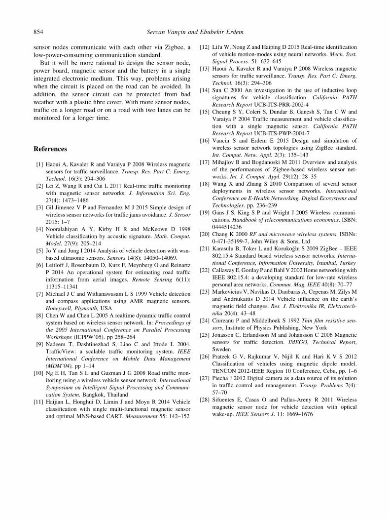
As another application for this part of the study, the

vehicles passing by Node 3 at the end of the 100-m road

were monitored every hour. The results were plotted

using Matlab software where the time 00:00 was taken as

the 0th hour and the time 23:00 as the 23rd. As can be

seen in figure 10, the number of vehicles passing by

between the 17th and the 18th hours was much higher

(135) than during the other time slots, and therefore,

traffic was considered heavy. In addition, the number of

vehicles passing by between the 4th and the 5th hours is

very much lower than during the other time slots and

therefore the traffic is considered mild. On the other

hand, according to figure 7, because the 7th, the 8th and

the 9th hours are morning working hours, the traffic

density was high. Compared with the other time slots,

during the 3rd, the 4th and the 5th, the traffic was mild,

because these are night hours. These results can be

shared with the drivers over the Internet if a server is

setup.

4.2 Vehicle classification

In this section, different from the studies by Haijian, L.,

Honghui et al and Lifu et al [11, 12], the types of the

vehicles were determined in four categories: cars,

Figure 6. Values coming from the nodes.

Figure 7. Number of vehicles–time plot with hourly intervals.

Implementation of the vehicle recognition systems 847

minibuses, buses and trucks. To make this detection, a more

precise and accurate measurement was needed and, there-

fore, an additional wireless sensor node was placed in the

middle of the road. In this application, again, the resultant

magnetic field (C) was calculated using Eq. (1). A magnetic

sensor was connected to the I2C port of the sensor node as

in the previous applications. The sensor circuit, which may

be considered an end node, transmits the magnetic data to

the node that was programmed as the communal node. The

ED converts the magnetic information in three axes (x,

y and z) to the resultant magnetic field using a program that

we wrote and transmits the value to the communal node

Table 2. MSL limiting values determined for the vehicle types.

Limit value for vehicle types MSLaverage

lc 3.5

lm 7.5

lb 14

lt 24

int main(void){ halInit(); printf("\n\r HMC5983L_TEST \n\r"); HMC5983LInit(); hmc.c=-999;

while(){ hmc.c=HMC5983L_Read(&hmc,0);

if(hmc.c!=-999){ printf("\n\r C:%d",(int)hmc.c);} else{

printf("\n\r error \n\r");} delayMs(90);}}

Figure 8. The code piece written in the Code Composer for the

magnetic sensor.

�me = 0

order_counter ++

Start

C > Cthreshold

F , �me_counter , vehicle_detec�on ,

order_counter

Calculate C value

F = 1 ;vehicle_detec�on = 1 ;

�me_counter ++ ;Calculate Cmax

F= 0; �me_counter = 0 ;

10 s

YN

M = ( Cmax – Cthreshold )t = �me_counter × 0.09

MSL = M × t

�me + = 0.09 sN

Y

lm < lblc < lm lb < lt

Car Detec�on Minibus Detec�on Bus Detec�on

Finish

lt

Truck Detec�on

MSL < lc

No Vehicle Detec�on

Figure 9. The flow diagram of the algorithm proposed for the vehicle classification (classification algorithm).

848 Sercan Vancin and Ebubekir Erdem

every 90 ms. Hence, the communal node sends the C value

for every 0.09 s to the Tera Term terminal, which has serial

port software. An HMC5983L magnetic sensor transmits

the data obtained to the communal node every 90 ms. In

figure 8, the code piece written in the hardware (hw.c) of

the magnetic sensor is shown.

Reducing this time interval will increase the sample size

of the magnetic data. Although an increase in the sample

size will deliver more significant and sensitive results, Tera

Term will not be able to obtain the data in that short time

interval. Therefore, the sampling time was determined as

90 ms, optimally.

In this application, the magnetic signature length MSLð Þwas identified to classify the vehicles. MSL can be calculated

with the help of the magnetic amplitude difference (DM) and

the occupation time (Dt) as in the following equation:

MSL ¼ DM � Dt ð2Þ

The magnetic amplitude difference is the difference

between the measured resultant field and the predetermined

threshold value. Occupation time, on the other hand, is the

time the vehicle stays in the coverage zone of the sensor

circuit. It is the product of the value given by the time

counter defined in the sensor code with 90 ms, because the

delay measurement method is adjusted to 90 ms. Depend-

ing on its MSL size, the vehicle type can be determined as

an automobile, a minibus, a bus or a truck. This depends on

the length and the mass of the metals it contains. Figure 9

shows the flow diagram of the algorithm proposed for

vehicle classification. One hundred vehicles consisting of

equal numbers of automobiles, minibuses, buses and truck

were made to pass by the sensors on the road in a random

order and the minimum limiting MSL values, lc; lm; lb and

lt (figure 9) for cars, minibuses, buses and trucks,

respectively, are shown in table 2. For example, lc is the

measured minimum MSL value for cars. On the other hand,

lm is both the maximum MSL value for cars and the min-

imum MSL value for minibuses. The important parameters

for determining these values were the coverage distance

between 0.5 and 0.75 m, the differences in length of dif-

ferent types of vehicles and the mass of the metal the

vehicle contains.

As seen in figure 9, if the C value was bigger than the

Cthreshold; then a vehicle was detected and the value of the

time counter was increased by 1. The flag value (F) that

declares the vehicle detection is coded as ‘‘1.’’ The order-

number parameter gives the number of measurements

made. The type of the vehicle can be determined with the

limiting values of MSL given in table 2.Figure 10. The car approaching the sensor circuit.

Figure 11. Resultant magnetic field–time plot (for car)

Figure 12. The minibus approaching the sensor circuit.

Implementation of the vehicle recognition systems 849

In this application, first, a car was made to pass by the

road at a constant speed of 40 km/s. It is known that a usual

car can have a length from 3.6 m to 5.0 m. Figure 10 shows

the car passing by the road.

Because the data were stored in the log part of the Tera

Term, only C values could be extracted by the data

extraction method of Matlab software. Those values were

examined with the Tera Term program every 0.09 s in a 10-

s period and the power boards of the sensors were shut

down to end the measurements. These values are also

plotted in figure 11. To clearly distinguish the detection

time interval and the C values, only values between the 2nd

and the 5th seconds are plotted. As shown in figure 11,

during the time interval Dt, vehicle detection was recorded

for six samples, meaning that the time-counter parameter

had the value 6. Because samples were taken once in

90 ms, the time interval can be found as Dt =

0.09 9 6 = 0.54 s. In addition, since the highest C value

for a passing vehicle was 262 and the Cthreshold was 255,

magnetic amplitude difference can be calculated as

DM = 262 - 255 = 7.

Thus, the magnetic signature length (MSL) for this car

could be found from Eq. (2), which gives 3.78. This value

is between lc and lm according to figure 9 and therefore the

detected vehicle was a car. The unit of the calculated MSL

value is of no importance; it just increases for minibuses or

buses.

Figure 13. Resultant magnetic field–time plot (for minibus).

Figure 14. The bus approaching the sensor circuit.

Figure 15. Resultant magnetic field–time plot (for bus).

Figure 16. A truck approaching the sensor circuit.

850 Sercan Vancin and Ebubekir Erdem

As a second application, measurements were made for a

minibus. Figure 12 shows the minibus approaching the

sensor circuit. Because the length of the minibus is com-

parable to that of the car, the occupation times during

passing by the sensor circuit were similar. But a minibus

contains more metal and therefore its magnetic amplitude

difference was higher than that of the car. Figure 13 shows

the results plotted using Matlab software.

Again, to clearly distinguish the detection time interval

and the C values, only values between the 5th and the 8th

seconds are plotted. As seen in figure 13, during the time

interval Dt, vehicle detection was recorded for seven

samples. This means the time-counter parameter had the

value 7. Because samples were taken once every 90 ms and

the highest C value for a passing by minibus was 272 and

the Cthreshold was 255, the magnetic signature length (MSL)

for the minibus can be found from Eq. (2), which gives

10.71. This value is between lm and lb according to figure 9

and therefore the detected vehicle was a minibus.

The third application was the detection of a city bus.

These buses are about 7–9 m long, so their occupation time

was longer than those of the cars or the minibuses. Fig-

ure 14 shows the bus approaching the sensor circuit. Fig-

ure 15 shows the data plotted for the bus. It can be seen

from the plot that the time-counter parameter was 9. Hence,

during the occupation time, nine samples measurements

were taken.

To clearly distinguish the detection time interval and the

C values, only values between the 4th and the 7th seconds

were plotted. As seen in figure 15, during the time interval

Dt vehicle detection was recorded for nine samples.

Because samples were taken once every 90 ms and the

highest C value for a passing by bus was 278 and the

Cthreshold was 255, the magnetic signature length (MSL) for

the bus can be found from Eq. (2), which gives 18.63. This

value is between lb andlt according to figure 9 and therefore

the detected vehicle was a bus.

Lastly, a truck was used for vehicle detection. Figure 16

shows a truck approaching the sensor circuit. During the

application many measurements were taken. The most

significant of the results are between 6th and 9th seconds

and are plotted in figure 17. The most important result here

is that the truck and the bus had similar magnetic amplitude

differences but different occupation times. Because the

detected truck was longer than the bus, its occupation time

in the coverage zone of the sensor node is longer.

Table 3. The average MSL values for every vehicle type.

Vehicle type MSLaverage

Car 5.23

Minibus 12.64

Bus 21.32

Truck 28.86

Table 4. Accuracies for the proposed vehicle classification algorithm.

Vehicle type The number of vehicles passed

The number of vehicles

detected

Accuracy of the proposed algorithm (%)Car Minibus Bus Truck

Car 25 24 1 0 0 96

Minibus 25 1 23 1 0 92

Bus 25 0 1 23 1 92

Truck 25 0 0 0 25 100

Total number of vehicles 100 24 23 23 25 95

95

Figure 17. Resultant magnetic field–time plot (for truck).

Figure 18. Direction determination scenario.

Implementation of the vehicle recognition systems 851

As seen in figure 17, during Dt, 14 samples of detection

were taken and the results were recorded. The time-counter

parameter was 14. Because samples were taken once every

90 ms and the highest C value for a passing truck was 280

and Cthreshold was 255, the magnetic signature length (MSL)

for the truck can be found from Eq. (2), which gives 31.5.

This value is bigger than lt according to figure 9 and,

therefore, the detected vehicle was a truck. Twenty-five

vehicles from each type passed along the road and the

average MSL values from the obtained data are summarised

in table 3. Table 4 shows the accuracy rates of the classi-

fication algorithm for 100 vehicles of different types.

According to table 4, the highest accuracy was attained for

trucks and the lowest accuracy for minibuses and buses,

with 100% and 92%, respectively. More significant, sen-

sitive and accurate results were obtained for trucks because

they are both large in size and rich in metal. On the other

hand, if all vehicles are taken into account, the average

accuracy is very high, with a rate of 95%.

4.3 Finding the direction of the vehicles

In this section, the direction of motion of the vehicles

passing by was determined. The direction of motion of the

vehicles can be from left to right or from right to left. In this

application, more than one sensor was used and the change

in the background magnetic field due to the vehicles

passing the sensors was measured in order to determine the

direction of motion in one direction [28]. Figure 18 gives

the application scenario for the determination of vehicle

direction. In this application, to determine the direction of

the vehicle, two sensor circuits were placed in the middle of

the road 5 m apart. The aim here is to observe if the change

in magnetic field was similar in the nodes placed nearby.

The direction is determined when the resultant magnetic

field C in one of the nodes exceeds the Cthreshold at a certain

time before the other node detects the vehicle.

�me =0

Start

SC1 SC2

No Vehicle Detected

�me += 0.09 sSC1 > 255

andSC1 > SC2

SC1 == SC2

SC2 > 255

Vehicle Direc�on = Le� to Right

�me 10 sN

Vehicle Direc�on = Right to Le�

N

N

Y

Finish

Y

Y

N

Y

Figure 19. Flow diagram of the algorithm proposed to deter-

mine the vehicle direction.

Figure 20. The vehicle approaching the sensor circuit.

Figure 21. Determination of the vehicle direction, from left to

right (resultant magnetic field (RMF)–time plot).

Figure 22. Determination of the vehicle direction, from right to

left (resultant magnetic field (RMF)–time plot).

852 Sercan Vancin and Ebubekir Erdem

As in the previous application, the measurement time

interval of the sensors was set to 90. Figure 19 shows the

flow diagram of the algorithm to determine the vehicle

direction. SC1 and SC2 parameters in the diagram are the C

values read at sensor 1 and sensor 2, respectively.

For this application, first, a car was made to pass by the

sensor circuits at a constant speed of 40 km/s as in fig-

ure 20. The direction on the x-axis is defined as from left to

right if the car travels from sensor 1 to sensor 2 and from

right to left otherwise.

Node 1 (sensor circuit 1) reported the existence of the

vehicle in a setting where samples were taken every 90 ms.

Soon after, Node 2 (sensor circuit 2) also reported the vehicle.

Hence, for a short period of time, Node 1 sent the logic value

1 and Node 2 sent the logic 0. Then, Node 1 sent the logic 0

and Node 2 sent the logic 1. These results were plotted with

Matlab software and are shown in figure 21.

As seen in figure 21, the vehicle was detected first by

sensor circuit 1 and then by sensor circuit 2. For example,

the highest magnetic field value detected by sensor circuit 1

was 263 and by sensor circuit 2 was 261. The occupation

times in the coverage zone of the sensor were also similar.

Because a flow from sensor circuit 1 to sensor circuit 2

was seen, the direction of the vehicle was determined as

from left to right. In addition to these, data acquired by the

sensor were similar. Therefore, one can conclude that the

same vehicle passed by the nodes.

The plot showing the vehicles travelling from right to left

is given in figure 22. It can be seen that the vehicle was first

detected by sensor node 2 and then sensor node 1 and

therefore it is determined that the vehicle was travelling

from right to left.

After that, a direction determination experiment was

performed with 50 vehicles; of which, 28 were travelling

from left to right and 22 were travelling from right to left.

As seen in table 5, an accuracy of 92.9% was attained for

vehicles travelling from left to right and 95.4% for the ones

travelling from right to left. In general, the system has an

accuracy of 94%.

5. Conclusion

In this study, three applications of vehicle detection by the

wireless magnetic sensors were developed and the results

are evaluated and analyzed with various software tools. In

the first of these applications, the traffic condition of 100 m

of a single-lane road was analysed for 30 min. In order to

perform this application, a power board, a magnetic sensor

and three sensor nodes with batteries were used. The aim

was to examine the traffic on 100 m by placing three sen-

sors 50 m apart. The traffic condition was classified with

respect to the traffic density as no traffic, mild traffic, heavy

traffic and very heavy traffic. With the obtained results,

instantaneous traffic density could be observed at every

second. In addition to these, with the information coming

from Node 3 placed at the end of the road, the vehicles

passing that section of road were counted all day and traffic

was analyzed hourly. This way, traffic density information

was determined with respect to the vehicles passing by per

minute.

In the second application, the vehicles travelling on the

road were categorised as four types: car, minibuses, buses

and trucks. In this classification, an MSL parameter was

proposed and used. As a result, the highest accuracy was

attained in the truck classification with a rate of 100%,

whereas the lowest accuracy was attained for the minibuses

and buses with a rate of 92%. In this application, more

significant, sensitive and accurate results were obtained for

trucks because they are both big in size and rich in metal.

But there were errors in differentiating minibuses and

buses.

Lastly, the direction of the vehicles was determined as

from left to right or from right to left. An accuracy of

92.9% was obtained for the vehicles travelling from left to

right and an accuracy of 95.4% was obtained for the ones

moving right to left. The performance of the algorithm for

the determination of the direction of vehicles was high and

the general accuracy rate turned out to be 94%. During the

applications, many experiments were performed with the

vehicles and samples were gathered from Tera Term soft-

ware. It was seen that the proposed algorithm gave more

accurate results with respect to the other studies.

These real-time results can be shared with the drivers in

the traffic simultaneously. In this way, drivers can obtain

information on the traffic condition (number, type and

direction of the vehicles).

The most important features of this study were learning

that the detection system is easy and more dynamic than the

systems in other studies and that the proposed method and

the algorithm deliver appropriate results. In addition, the

number of hardware elements is few and low cost and the

Table 5. Accuracies for the proposed algorithm of vehicle direction determination.

Direction of vehicle The number of vehicles passed

The number of vehicles

detected

Accuracy of the proposed algorithm (%)Left to right Right to left

Left to right 28 26 2 92.9

Right to left 22 1 21 95.4

Total number of vehicles 50 26 21 94

Implementation of the vehicle recognition systems 853

sensor nodes communicate with each other via Zigbee, a

low-power-consuming communication standard.

But it will be more rational to design the sensor node,

power board, magnetic sensor and the battery in a single

integrated electronic medium. This way, problems arising

when the circuit is placed on the road can be avoided. In

addition, the sensor circuit can be protected from bad

weather with a plastic fibre cover. With more sensor nodes,

traffic on a longer road or on a road with two lanes can be

monitored for a longer time.

References

[1] Haoui A, Kavaler R and Varaiya P 2008 Wireless magnetic

sensors for traffic surveillance. Transp. Res. Part C: Emerg.

Technol. 16(3): 294–306

[2] Lei Z, Wang R and Cui L 2011 Real-time traffic monitoring

with magnetic sensor networks. J. Information Sci. Eng.

27(4): 1473–1486

[3] Gil Jimenez V P and Fernandez M J 2015 Simple design of

wireless sensor networks for traffic jams avoidance. J. Sensor

2015: 1–7

[4] Nooralahiyan A Y, Kirby H R and McKeown D 1998

Vehicle classification by acoustic signature. Math. Comput.

Model. 27(9): 205–214

[5] Jo Y and Jung I 2014 Analysis of vehicle detection with wsn-

based ultrasonic sensors. Sensors 14(8): 14050–14069.

[6] Leitloff J, Rosenbaum D, Kurz F, Meynberg O and Reinartz

P 2014 An operational system for estimating road traffic

information from aerial images. Remote Sensing 6(11):

11315–11341

[7] Michael J C and Withanawasam L S 1999 Vehicle detection

and compass applications using AMR magnetic sensors.

Honeywell, Plymouth, USA

[8] Chen W and Chen L 2005 A realtime dynamic traffic control

system based on wireless sensor network. In: Proceedings of

the 2005 International Conference on Parallel Processing

Workshops (ICPPW’05). pp 258–264

[9] Nadeem T, Dashtinezhad S, Liao C and Iftode L 2004.

TrafficView: a scalable traffic monitoring system. IEEE

International Conference on Mobile Data Management

(MDM’04), pp 1–14

[10] Ng E H, Tan S L and Guzman J G 2008 Road traffic mon-

itoring using a wireless vehicle sensor network. International

Symposium on Intelligent Signal Processing and Communi-

cation System. Bangkok, Thailand

[11] Haijian L, Honghui D, Limin J and Moyu R 2014 Vehicle

classification with single multi-functional magnetic sensor

and optimal MNS-based CART. Measurement 55: 142–152

[12] Lifu W, Nong Z and Haiping D 2015 Real-time identification

of vehicle motion-modes using neural networks. Mech. Syst.

Signal Process. 51: 632–645

[13] Haoui A, Kavaler R and Varaiya P 2008 Wireless magnetic

sensors for traffic surveillance. Transp. Res. Part C: Emerg.

Technol. 16(3): 294–306

[14] Sun C 2000 An investigation in the use of inductive loop

signatures for vehicle classification. California PATH

Research Report UCB-ITS-PRR-2002-4

[15] Cheung S Y, Coleri S, Dundar B, Ganesh S, Tan C W and

Varaiya P 2004 Traffic measurement and vehicle classifica-

tion with a single magnetic sensor. California PATH

Research Report UCB-ITS-PWP-2004-7

[16] Vancin S and Erdem E 2015 Design and simulation of

wireless sensor network topologies using ZigBee standard.

Int. Comput. Netw. Appl. 2(3): 135–143

[17] Mihajlov B and Bogdanoski M 2011 Overview and analysis

of the performances of Zigbee-based wireless sensor net-

works. Int. J. Comput. Appl. 29(12): 28–35

[18] Wang X and Zhang S 2010 Comparison of several sensor

deployments in wireless sensor networks. International

Conference on E-Health Networking, Digital Ecosystems and

Technologies. pp. 236–239

[19] Gans J S, King S P and Wright J 2005 Wireless communi-

cations. Handbook of telecommunications economics. ISBN:

0444514236

[20] Chang K 2000 RF and microwave wireless systems. ISBNs:

0-471-35199-7, John Wiley & Sons, Ltd

[21] Karasulu B, Toker L and Korukoglu S 2009 ZigBee – IEEE

802.15.4 Standard based wireless sensor networks. Interna-

tional Conference, Information University, Istanbul, Turkey

[22] Callaway E, Gorday P and Bahl V 2002 Home networking with

IEEE 802.15.4: a developing standard for low-rate wireless

personal area networks. Commun. Mag. IEEE 40(8): 70–77

[23] Markevicius V, Navikas D, Daubaras A, Cepenas M, Zilys M

and Andriukaitis D 2014 Vehicle influence on the earth’s

magnetic field changes. Res. J. Elektronika IR, Elektrotech-

nika 20(4): 43–48

[24] Ciureanu P and Middelhoek S 1992 Thin film resistive sen-

sors, Institute of Physics Publishing, New York

[25] Jonasson C, Erlandsson M and Johansson C 2006 Magnetic

sensors for traffic detection. IMEGO, Technical Report,

Sweden

[26] Prateek G V, Rajkumar V, Nijil K and Hari K V S 2012

Classification of vehicles using magnetic dipole model.

TENCON 2012-IEEE Region 10 Conference, Cebu, pp. 1–6

[27] Piecha J 2012 Digital camera as a data source of its solution

in traffic control and management. Transp. Problems 7(4):

57–70

[28] Sifuentes E, Casas O and Pallas-Areny R 2011 Wireless

magnetic sensor node for vehicle detection with optical

wake-up. IEEE Sensors J. 11: 1669–1676

854 Sercan Vancin and Ebubekir Erdem