Implementation, Validation and Application of the 3GPP3D MIMO Channel Model in Open Source Simulation Tools
Fjolla Ademaj, Martin Taranetz, Markus Rupp
Vienna University of Technology, Institute of TelecommunicationsGusshausstrasse 25/389, A-1040 Vienna, Austria
Email: {fademaj, mtaranet, mrupp}@nt.tuwien.ac.at
Abstract—Beamforming and Multiple Input Multiple Output(MIMO) have been identified as key technologies to meet the everincreasing capacity demands in future mobile cellular networks.So far, these features have mainly been investigated in theazimuth dimension, considering one-dimensional antenna arrays.Recently, the 3rd Generation Partnership Project has released anew 3-dimensional (3D) spatial channel model that also accountsfor the elevation. It supports two-dimensional antenna arraysand enables to scrutinize concepts such as elevation beamformingand Full Dimension-Multiple Input Multiple Output. However,existing studies have mainly been carried out with commercialtools, thus largely limiting their reproducibility. This paperprovides a guideline for the practical implementation of the 3Dchannel model into existing link- and system level simulationtools. Considering the complexity of the model itself, our mainfocus is on computational efficiency. We validate our approachwith the Vienna LTE-A Downlink System Level Simulator andpresent simulation examples with various planar antenna arraysand polarization schemes.
Index Terms—3GPP 3D channel model, system level simula-tions, link level simulation, open source, elevation beamforming,full dimension-MIMO, vertical sectorization, channel coefficientgeneration
I. INTRODUCTION
Developing realistic channel models is one of the great-est challenges in describing wireless communications. Theirquality is crucial for accurately predicting the performance ofa wireless cellular system. Channel models can be broadlydivided into two categories, deterministic and stochastic. De-terministic models describe the channel for a specific prop-agation environment between transmitter and receiver. Sincethis method can be tedious to evaluate and does not allowfor general statements in an ensemble of environments, thechannel characteristics are often condensed to a statisticaldescription, e.g., the typical Power Delay Profile (PDP).
In order to close the gap between the two approaches, 3rdGeneration Partnership Project (3GPP) introduced the SpatialChannel Model (SCM) [1]. This model represents scatterersthrough statistical parameters without being physically po-sitioned. It is also known as a geometric stochastic modeland separately defines large scale parameters (e.g., shadowfading, delay spread and angular spreads) as well as smallscale parameters (e.g., delays, cluster powers, and arrival-and departure angles). Both parameter sets are randomly
drawn from tabulated distributions. The large scale parametersincorporate the geometric positions of the Base Stations (BSs)and the Users (UEs), and are used to parameterize the statisticsof the small scale parameters. Then, the channel behavior isdefined based on the PDP and the Angular Profile (AP).
The SCM model in [1] includes six different scenarios,each of them representing a unique environment. Since it wastargeted for a bandwidth of only 5MHz, and a carrier fre-quency of 2GHz, 3GPP extended this model to the so-calledSpatial Channel Model Extended (SCME). It follows the sameprocedure as SCM but supports bandwidths of up to 100MHzand a frequency range of 2 − 6GHz. In the course of theWireless World Initiative New Radio (WINNER) projects, themodel was extended for 15 different scenarios [2, 3], includingurban-, rural- and moving environments. The WINNER modelis also recommended as a baseline for the evaluation of radiointerface technologies in the International TelecommunicationUnion - Radiocommunication Sector (ITU-R) [4].
All models presented above are limited to the azimuthdimension. Thus, when it comes to describing Multiple InputMultiple Output (MIMO) systems, only linear antenna arraysin the horizontal direction are supported. As interest in 3-dimensional (3D) beamforming is greatly increasing, enablingconcepts such as Full Dimension (FD)-MIMO and verticalsectorization, modeling the elevation direction is becomingindispensable. Recently, 3GPP introduced a new 3D SCM forLTE-Advanced (LTE-A) [5].
Yet, only few simulation studies, including reports fromthe 3GPP TSG RAN WG1 meetings, have been publishedthat claim the practical implementation of the model [6, 7].However, the employed tools are mainly developed by net-work operators and vendors, and thus typically intended forcommercial use. The authors believe that open access isa key prerequisite for reproducible simulation studies. Thispaper is the first to provide a guideline for the practicalimplementation of the model. The MATLAB source codeis openly available for download on our webpage www.nt.tuwien.ac.at/vienna-lte-a-simulators under an academic, non-commerical use license. It is provided as a stand-alone packagethat is directly applicable for system level simulation tools andcan straightforwardly be ported to link level.
2015 International Symposium on Wireless Communication Systems (ISWCS), 25-28 Aug. 2015
Set scenario, network layout and
antenna parameters
Generate XPRs Perform random coupling of rays
Generate arrival & departure angles
Generate cluster powers
Generate delays
Assign propagation condition (NLOS/
LOS)Calculate pathloss
Generate correlated large scale
parameters (DS, AS, SF, K)
Draw random initial phases
Generate channel coefficient
Apply pathloss and shadowing
General parameters:
Small scale parameters:
Coefficient generation:
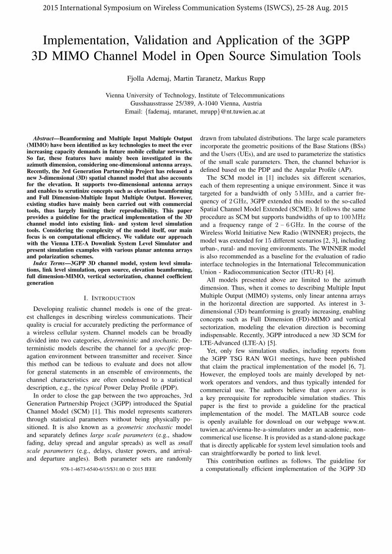
Fig. 1: Procedure for generating coefficients of fast fadingMIMO channel as defined in [5].
channel model is presented in Section II. In Section III, theimplementation is validated against results from the 3GPPstandard with the Vienna LTE-A Downlink System LevelSimulator. While 3GPP provides the specifications for the new3D channel model, parametrization examples for specific testcases and transmission scenarios currently seem to be missing(April 2015). We provide a few parameter sets within thispaper that we experienced as typical in the past. Moreover,simulation results for various planar antenna array patternsand polarization schemes are provided. Section IV outlinesnew opportunities for investigations and Section V concludesthe work.
II. 3D CHANNEL MODEL IN SYSTEM LEVEL SIMULATOR
In this section, we describe the necessary steps to integratethe 3D channel model into an existing simulation tool. Thetarget is to compute a NRx × NTx MIMO-channel matrixH(t, f) for each sampling point on the time-frequency grid1,where NTx and NRx denote the number of transmit- andreceive antenna ports, respectively.
In the 3D channel model, the channel coefficients are largelydependent on the UE location in the 3D space and, thus,have to be calculated at runtime. Hence, the challenge is toperform computationally intensive tasks off-line or on demand,whenever possible. We will follow the stepwise procedure2 asspecified in [5, Sec. 7.3] and illustrated in Figure 1, and explainits expedient partition for implementation.
[GP] The first step is to generate the general parameters.It starts with setting the network layout, the scenario environ-ment and the antenna array parameters (Step 1). Currently, thestandard specifies two scenarios, 3D-Urban Macro cell (UMa)and 3D-Urban Micro cell (UMi), and various planar antennaarray structures, defining the location and polarization of eachantenna element, as well as the element-to-port mapping. The
1On link level, channel realizations are typically calculated per OFDMsymbol and LTE-A subcarrier [8]. On system level, they are commonlygenerated per physical Resource Block (RB) [9].
2The steps are denoted as ’Step N’ with N∈ {1, ..,12}.
next steps are to assign the propagation conditions (Step 2),i.e., either Line of Sight (LOS) or Non-Line of Sight (NLOS),calculate the experienced path loss (Step 3) and generate thelarge scale parameters3 (Step 4) for each 3D location withinthe region of interest. These tasks can be performed off-line,i.e., before entering the actual simulation loop. Similar to thegeneration of the shadow fading, they have to be carried outonly once per eNodeB site.
[SSP] The next step is to generate small scale parameters.In the 3D channel model, channel coefficients Hu,s,n(t, f) aredetermined individually for each cluster n and each receiver-and transmitter antenna element pair {u, s}, respectively. Thecalculation of Hu,s,n(t, f) requires to generate delays (Step5), cluster powers (Step 6) as well as arrival- and departureangles for both azimuth and elevation (Step 7). After couplingthe rays within a cluster (Step 8), Cross Polarization PowerRatios (XPRs) and random initial phases are drawn (Step 9and 10). Together with the calculation of the spherical unitvectors and the Doppler frequency component (both Step 11),all parameters mentioned above are commonly applied to eachantenna element pair {u, s} and thus have to be determinedonly once per antenna array and physical RB. The latteraccounts for the frequency-selectivity of the channel.
[CG] The final channel matrix H(t, f) is obtained byfirst aggregating the channel coefficients of all clusters n ofan individual pair {u, s}, i.e., Hu,s(t, f) = ∑nHu,s,n(t, f),and then combining the cumulative channels according tothe antenna element-to-port mapping, i.e., [H(t, f)]m,n =∑u∈Pm
ωu∑s∈PnωsHu,s(t, f), where Pm and Pn denote the
sets of antenna elements that belong to receive antenna portm and transmit antenna port n, and ωu and ωs are complexweights that account for phase shifts as applied for staticbeamforming (e.g., electrical downtilting), respectively.
Considering a UE with a fixed location in the 3D space,[SSP] and [CG] have to be carried out only in the first timeinstant of the simulation. Afterwards, the channel will remainstatic over time (no Doppler). If the UE moves at a certainspeed, represented by the vector v ∈ R3, in principle, [SSP]and [CG] would have to be performed at runtime in each timeinstant of the simulation. This also implies the generationof new clusters and random initial phases, i.e., a completechange of the multi-path propagation environment. Thus, itis considered reasonable from a physical perspective (see,e.g., [3]) as well as in view of computational complexity topartition the scenario into equally sized cubes. As long as theUE resides within the same cube, it is assumed to experiencethe same path loss, shadow fading, propagation conditions(LOS/NLOS) and large scale parameters, as generated in [GP].Then, [SSP] has to be carried out only once at the beginningof the simulation and each time the UE transfers to another
3The vector of large scale parameters incorporates shadow-fading, theRicean K-factor (only in the LOS case), delay-spread, azimuth angle spreadof departure- and arrival, as well as zenith angle spread of departure- andarrival. The latter have become available not until the introduction of the 3Dchannel model.
1 m
UE
1 m
1 m
z
x
y
v
Fig. 2: UE travels through cube with an edge length of 1m.
cube4. Within a cube, channel variations are caused by theslightly changing angles of arrival and departure (and thus theantenna element field patterns) as well as the phase shift due tothe Doppler. They can be incorporated into [CG], thus yieldingthe only variable components that have to be recalculated ineach time instant of the simulation.
III. CALIBRATION AND SIMULATION EXAMPLES
Following the steps in Section II, we incorporated the3D channel model in the Vienna LTE-A Downlink SystemLevel Simulator (current version v1.8r1375) [9]. The sim-ulator is implemented in object-oriented MATLAB and ismade openly available for download under an academic, non-commercial use license. It is built according to the commonlyemployed structure for system level simulation tools (see, e.g.,in [10, 11]), as illustrated in Figure 3, thus serving as arepresentative example. Its centerpiece is the link abstractionmodel that specifies the interaction between link- and systemlevel simulations [9, 10]. This structure is expected to persistin simulation tools for the fifth generation of mobile cellularnetworks (5G) [11]. The enhancements that were necessary toenable the 3D channel model are depicted by the boxes shadedin gray at the top of the figure.
A. Calibration
For calibration purposes, we carry out simulations with thesetup as specified in [5, Table 8.2-2]. The setup is summarizedin Table I. Two scenarios, 3D-UMa and 3D-UMi are inves-tigated. They represent typical urban macro-cell- and micro-cell environments. While the former consider a BS height of(25m), surpassing the surrounding buildings, the latter specifya BS height of (10m), thus lying below the rooftop level.Moreover, all parameters for computing path loss, shadowfading, large scale parameters and small scale fading arespecifically defined for each scenario. Both 3D-UMa and 3D-UMi are assumed to be densely populated with buildings andtake into account both indoor- and outdoor UEs. Figure 4depicts the obtained statistics of the large scale parametersas generated for each UE based on Step 4 (conf. Section II).
4Assuming a spatial resolution of 1m and a temporal resolution of 1ms,referring to the length of one LTE sub-frame, also denoted as TransmissionTime Interval (TTI), a UE moving at v = [27.78,0,0]m/s requires 36msto travel from one face of the cube to the other, as indicated in Figure 2. Inthis case, [SSP] is called every 36 sub-frames.
network layout
path loss
shadow fading
LO
S/N
LO
S
positiondependent
small-scale fadingenvironment
antenna field
large scale parameters
time-dependent
antenna arrayparameters
link performancemodel
link quality model
throughput
BLER
precoding
power allocation
HARQ
Block Size
modulation
& coding
assigned PHY
resources
sched
uling
traffic model
QoS
link
adaptation
strategy
post-equalizationSINR
link ab
straction m
odel
Fig. 3: Enhanced link abstraction model for enabling 3Dchannel modeling.
TABLE I: Simulation parameters for calibration as referredfrom [5].
Antenna elements per port M = 10Vertical antenna element spacing λ/2
Horizontal antenna element spacing λ/2Maximum antenna element gain 8dBi
Electrical downtilt 12○
UE distribution uniform in cell [5]
The parameters incorporate the spatial-correlation among UEsserved by the same eNodeB as well as cross-correlationsamong the parameters themselves. In accordance with theresults in [12], the distributions show similar characteristics for3D-UMa and 3D-UMi. It is further observed that they showa good agreement with results from [5] (dash-dotted curves)that were obtained by averaging over 21 sources5.
B. Simulation Examples
In this section we consider a network with seven macrosites, each employing three eNodeBs, and simulate 50 ran-domly distributed UEs per eNodeB sector. Our goal is tocompare the throughput performance for various antenna arrayconfigurations at the eNodeB. We consider four antenna ports,i.e., NTx = 4, and compare linear and cross-polarized antenna
5In the calibration part of [5], results are only provided for the zenith anglespreads.
3D-UMa 3D-UMi
Shadow Fading [dB]-25 -15 -5 5 15 25
ECD
F
0
0.2
0.4
0.6
0.8
1
(b) Shadow fading
Delay Spread [s] ×10-50 0.2 0.4 0.6 0.8 1
ECD
F0
0.2
0.4
0.6
0.8
1
(c) Delay spread
Azimuth Spread of Departure [°]80 100 120
ECD
F
0
0.2
0.4
0.6
0.8
1
0 20 40 60
(d) Azimuth spread of departure
Azimuth Spread of Arrival [°]0 100 120
ECD
F
0
0.2
0.4
0.6
0.8
1
20 40 60 80
(e) Azimuth spread of arrival
Zenith Spread of Departure [°]0
ECD
F
0
0.2
0.4
0.6
0.8
1
10 3020 40 50 60
(f) Zenith spread of departure
Zenith Spread of Arrival [°]0
ECD
F
0
0.2
0.4
0.6
0.8
1
10 4020 30 50 60
(g) Zenith spread of arrival
Fig. 4: Large scale parameter statistics. Solid lines refer toresults 3D-UMa and 3D-UMi scenario. Dashed curves denotereference results from [5].
element arrangements6, further denoted as Config 1 and Config2, respectively. Secondly, we vary the antenna array geometry,assuming setups with M = 2 and M = 10 antenna elementsper antenna port, as indicated in Figure 5. The UEs areequipped with a single linearly polarized antenna element thatis attached to a single antenna port. The simulation setup issummarized in Table II.
Figure 6 depicts simulation results in terms of average UEthroughput statistics. It is observed that, remarkably, Config1achieves an almost two-times higher throughput than Config2,just by employing the same polarization direction as the UE.Moreover, it is seen that using M = 2 instead of M = 10antenna elements per column decreases the performance. Thisis mainly caused by the fact that with M = 10 elements in thevertical direction, a sharper static beam can be achieved by
6The slant angle is incorporated by using Polarization Model-2 from[5, Sec. 7.1.1], as this model yields the best agreement with results frommeasurements [13].
...
...
...
...
...
Config 1 Config 2
eNodeB UE
M=
{2,1
0}
p0
p2
p1
p3
p0
p2
p1
p3
λ/2
λ/2
λ/2λ/2
ω1(θtilt)
ωΜ(θtilt)
ω1(θtilt)
ωΜ(θtilt)
Fig. 5: Antenna array configurations. The antenna ports aredenoted as pi with i ∈ {1, . . . ,4}, and ωj , j ∈ {1, . . . ,M}are the phase shifts for static beamforming (e.g., electricaldowntilting).
Traffic model full bufferSimulation length 50 TTIs
Number of simulation runs 20
the electrical down-tilting. The figure further shows separatestatistics for LOS- and NLOS UEs for each scenario. It isseen that UEs in LOS achieve a considerably better throughputperformance than in NLOS. Remarkably, the width of the gapdepends on the polarization scheme and the number of antennaelements per column.
IV. NEW OPPORTUNITIES
The integration of the 3D channel model into existing link-and system level simulation tools paves the way for moreadvanced studies on the performance of a mobile cellularsystem in realistic environments. Existing channel modelsonly supported linear antenna arrays in the azimuth. Withthe introduction of the third dimension, not only higher-order MIMO schemes but also higher number of antennaelements per antenna array can be investigated. Currently, the
Average UE throughput [Mbit/s]0.1 0.2 0.3 0.4 0.5 0.6 0.7
EC
DF
0
0.1
0.2
0.3
0.4
0.5
0.6
0.7
0.8
0.9
1
0
Config 2, M=2
Config 2, M=10
Config 1, M=10
Average
LOS
NLOS
Fig. 6: Average UE throughput [Mbit/s] ECDF curves for vari-ous antenna polarization schemes and antenna array structures.Solid lines depict typical throughput. Dashed and dotted linesshow performance as achieved by LOS and NLOS UEs.
3GPP LTE-A standard supports up to eight antenna ports.However, current trends aim at 100 and more antenna ports pereNodeB [14]. A main enabler for this so called massive MIMOapproach will be the adoption of higher carrier frequencies,also termed millimeter-wave communication, as it enables toconsiderably decrease the size of the antenna arrays. On theone hand, this may lead to higher complexity of the hardware,larger energy consumption and a greater demand for signalprocessing capabilities. On the other hand, it will enable amuch more accurate bundling of energy towards the intendedreceiver, which is a key prerequisite for aggressive frequencyreuse. In dense urban environments, where UEs move in threedimension (consider, e.g., shopping malls, skyscrapers, andmore) it is conceivable that the spectral efficiency per unitsphere might replace the area spectral efficiency as a figure ofmerit. Other important use cases are scenarios with high usermobility, as the number of commuters is expected to increasesubstantially. People have become used to services followingthem wherever they travel. Mobile cellular access has evenbecome a key argument to choose the means of transportation.Sharp, steerable beams might be an expedient solution to thisissue, as they could follow a vehicle along its path.
V. CONCLUSION
This paper presented a guideline for the practical im-plementation of the 3GPP 3D channel model into existinglink- and system level simulation tools. We met the chal-lenge of calculating the channel coefficients at simulationruntime by carefully partitioning the step-wise procedure asproposed by the 3GPP. We demonstrated the validity of ourapproach by integrating it into the Vienna LTE-A DownlinkSystem Level Simulator. The obtained large scale parametersstatistics showed a good agreement with the results whichare provided by the 3GPP for calibration. We carried out
example simulations with various antenna array setups andobserved a strong impact of the antenna polarization on thetypical UE performance. We completed the work with anelaboration on new opportunities that became possible withthe 3D channel model. Our hope is to inspire researches anddevelopers of link- and system level simulation tools to furtherelaborate on these topics by directly applying or reusing ourimplementation approach.
ACKNOWLEDGMENTS
This work has been funded by the Christian Doppler Lab-oratory for Wireless Technologies for Sustainable Mobility,the A1 Telekom Austria AG, and the KATHREIN-Werke KG.The financial support by the Federal Ministry of Economy,Family and Youth and the National Foundation for Research,Technology and Development is gratefully acknowledged.
[2] WINNER I WP5, “Final report on link level and systemlevel channel models,” IST-2003-507581 WINNER I DeliverableD5.4, Nov. 2005.
[3] WINNER II WP1, “WINNER II channel models,” IST-4-027756WINNER II Deliverable D1.1.2, Sept. 2007.
[4] M. ITU-R, “Guidelines for evaluation of radio interface tech-nologies for IMT-Advanced,” Report, Dec. 2009.
[5] 3rd Generation Partnership Project (3GPP), “Study on 3Dchannel model for LTE,” 3rd Generation Partnership Project(3GPP), TR 36.873, Sept. 2014.
[6] A. Kammoun, H. Khanfir, Z. Altman, M. Debbah, andM. Kamoun, “Preliminary results on 3D channel modeling:From theory to standardization,” IEEE Journal on SelectedAreas in Communications, vol. 32, no. 6, pp. 1219–1229, June2014.
[7] Z. Hu, R. Liu, S. Kang, X. Su, and J. Xu, “Work in progress:3D beamforming methods with user-specific elevation beam-foming,” in International Conference on Communications andNetworking in China (CHINACOM), Aug. 2014, pp. 383–386.
[8] S. Schwarz, J. Ikuno, M. Simko, M. Taranetz, Q. Wang, andM. Rupp, “Pushing the limits of LTE: A survey on researchenhancing the standard,” IEEE Access, vol. 1, pp. 51–62, 2013.
[9] M. Taranetz, T. Blazek, T. Kropfreiter, M. Muller, S. Schwarz,and M. Rupp, “Runtime precoding: Enabling multipoint trans-mission in LTE-Advanced system level simulations,” acceptedfor revision in IEEE Access, 2015.
[10] S. Ahmadi, LTE-Advanced: A Practical Systems Approach toUnderstanding 3GPP LTE Releases 10 and 11 Radio AccessTechnologies, ser. ITPro collection. Elsevier Science, 2013.
[11] Y. Wang, J. Xu, and L. Jiang, “Challenges of system-level sim-ulations and performance evaluation for 5G wireless networks,”IEEE Access, vol. 2, pp. 1553–1561, 2014.
[12] 3GPP TSG RAN WG-1, “R1-140048: Phase 2 calibration re-sults for 3D channel model,” 3rd Generation Partnership Project(3GPP), Tech. Rep., Feb. 2014.
[14] F. Rusek, D. Persson, B. K. Lau, E. Larsson, T. Marzetta,O. Edfors, and F. Tufvesson, “Scaling up MIMO: Opportunitiesand challenges with very large arrays,” IEEE Signal ProcessingMagazine, vol. 30, no. 1, pp. 40–60, Jan. 2013.


![Ray-Tracing based Validation of Spatial Consistency for ... · in 3GPP 3D model [8]. Figure 1 illustrates one example of an urban environment used in the ray-tracing simulator. The](https://static.documents.pub/doc/80x56/5fd89146f4c52f40824fa331/ray-tracing-based-validation-of-spatial-consistency-for-in-3gpp-3d-model-8.jpg)


